Semiclassical analysis of Bose-Hubbard dynamics

Abstract

In this work the two site Bose-Hubbard model is studied analytically in the limit of weak coupling $u$ and large number of particles $N$. The semiclassical approximation where $\frac{1}{N}$ plays the role of Planck’s constant was used and perturbation theory to order $u^{2}$ was applied. In particular, the difference in the occupation between the two sites, where initially all particles are at one site was calculated analytically. Excellent agreement with the exact numerical solution was found. This quantity exhibits collapses and revivals that superimpose rapid oscillations. The occupation difference was calculated also for the case where initially both sites are occupied provided that the difference in occupation is sufficiently large. It provides an analytical description of results that were so far found only numerically. Similar behavior and analysis are expected for a large variety of physical situations in optics, atom optics and quantum dynamics of electrons in Rydberg atoms.

I introduction

The physics of Bose-Einstein condensates (BECs) is extensively studied in the recent years Pita_book ; PS_review ; Pethick@Smith . For weakly coupled atoms in a large variety of systems the Gross-Pitaevskii equation (GPE) Pita_book ; Pethick@Smith describes well the static properties. For the dynamics, the situation is more complicated and it is instructive to study simple paradigmatic systems. For the double well potential, the GPE does not reproduce the correct dynamics. In particular, the collapse of the amplitude of Rabi oscillations as a function of time is not reproduced, in contradiction with the numerical solutions for the many-body system Milburn ; ODell2 . The double well is a paradigmatic model system that was extensively studied experimentally Obert_exp ; jeff ; shin ; dorond . Much interest was in the Bosonic Josephson effect Obert_exp ; jeff . This is a clear manifestation of macroscopic quantum coherence. It encourages theoretical exploration of this and related systems Milburn ; Doron ; Smerzi ; Spekkens&Sipe ; ReinhardtPRL . If the inter-particle interaction is sufficiently weak so that the coupling between the lowest levels of the double well and higher levels can be ignored, the system may be described by the two site Bose Hubbard (BH) model where bosons can occupy only two sites Assa . This model has been studied numerically and analytically Milburn ; Doron ; Ofir_DW ; OfirDW ; Obert_the ; ODell ; Ofir_BH ; Kuklov4 . Fascinating phenomena that were explored are collapse and revival of the difference in the occupation of the sites Milburn ; and the semiclassically-related statistics of the fluctuations that are associated with the occupation dorona ; doronb ; Doron . The latter are important for the fringe visibility in interference experiments dorond . The understanding of the revivals is crucial for understanding of the coherence in the system.

Collapses and revivals were observed in experiments where a BEC was confined to a lattice. The interference pattern of the matter wave field originating in different lattice sites showed collapses and revivals as a function of time Bloch_colapse ; Bloch_ex . These were found also experimentally for other condensates Deepak ; Deepak2 and Rydberg atoms of2 ; of3 . Coherence was explored for models of dynamics of atoms on optical lattices in Fisher3 ; Fisher4 . Collapses and revivals were found in numerical calculations following heuristic arguments and in direct numerical studies of the double well problem OfirDW ; Ofir_DW ; ODell2 . For the two site Bose-Hubbard model, collapses were found in exact numerical calculations Ofir_DW ; OfirDW . Collapses and revivals were found theoretically for interacting bosons in a harmonic well and the relevant times were estimated Lewenstein ; Wright ; wright&walls ; castin&dalibard ; You . These were found also for wave packets in harmonic wells with small nonlinearities Mark . In quantum optics these were found in the Jaynes-Cummings model Jaynes_model analytically and numerically Eberly . It is the closest to the one found in the present paper for interacting bosons. In optics this phenomenon is well understood and is known as the Talbot effect Talbot ; Rayleigh (see also carpet ; Berry_box ). A related phenomenon is the “Quantum carpet” Berry&Sclich ; Berry_box . Collapses and revivals can be found in many situations. A generic picture is outlined in of1_pit ; PS_review .

A semiclassical picture for the two site Bose-Hubbard model was developed and studied in some detail Obert_the ; Milburn ; Doron . The dimensionless parameter that controls the corresponding classical behavior is

$$u=\frac{UN}{J}$$ (1)

where $U$ is the inter-particle interaction, $J$ is the strength of the hopping between the sites, while $N$ is the number of particles. In this picture, $\frac{1}{N}$ plays the role of Planck’s constant and the thermodynamic limit $N\rightarrow\infty$ plays the role of the classical limit. The various regimes are Doron :

1. Rabi regime $u<1$

2. Josephson regime $1<u<N^{2}$

3. Fock regime $N^{2}<u$.

The Josephson regime is the most extensively studied one ODell ; Obert_the ; Doron . It exhibits an interesting phase space, with dynamics related to the experimental observations Obert_exp ; jeff . We confine ourselves to the Rabi regime where the classical behavior is very simple. It enables us to study analytically quantum collapses and revivals that are crucial in the understanding of coherence.

The present work will follow the formulation presented in detail in the work of D. Cohen and coworkers Doron . In the limit $N\gg 1$ we find an analytical formula for the difference between the occupation of the two sites. It is rare to find such results for interacting systems and to the best of our knowledge it is the first time such an analytic expression is found in the present context, namely for interacting bosons.

The outline of the paper is as follows: In section II the model is defined and the semiclassical picture is presented. In section III a transformation to angle action variables is performed and used to find the energies within the WKB approximation to the order $u^{2}$, and in section IV it is calculated in standard quantum perturbation theory. In section V the difference in occupation between the two sites is calculated for an initial condition where all atoms are on one site, while in section VI the initial condition where both sites are occupied is used. The results are discussed in Sec. VII.

II The two states Hubbard model

The two states Hubbard model we study is defined by the Hamiltonian

$$H_{BH}=-J\left(a_{L}^{\dagger}a_{R}+a_{R}^{\dagger}a_{L}\right)+U\left[n_{L}\left(n_{L}-1\right)+n_{R}\left(n_{R}-1\right)\right].$$ (2)

The sites are denoted by $L$ (Left) and $R$ (Right). The creation and annihilation operators on the sites are $a_{L}^{\dagger},a_{R}^{\dagger}$ and $a_{L},a_{R}$ . The number operators for the two sites are $n_{L}=a_{L}^{\dagger}a_{L}$ and $n_{R}=a_{R}^{\dagger}a_{R}$. The commutation relations are $\left[a_{L},a_{L}^{\dagger}\right]=1$, $\left[a_{R},a_{R}^{\dagger}\right]=1$, and the units are such that $\hbar=\frac{1}{N}$. It is assumed that the on site energies on the two sites are identical. The total number of particles $n_{L}+n_{R}=N$ is conserved. The first term in (2) represents the hopping between the two sites while the second one is the energy of the interparticle interaction that in the present work is assumed to be small. The Hamiltonian (2) can be written in the form

$$H_{BH}=-J\left(a_{L}^{\dagger}a_{R}+a_{R}^{\dagger}a_{L}\right)+U\left(a_{R}^{\dagger}a_{R}^{\dagger}a_{R}a_{R}+a_{L}^{\dagger}a_{L}^{\dagger}a_{L}a_{L}\right).$$ (3)

By using the angular momentum operators (see for example Doron )

$$\begin{array}[]{ccl}S_{x}&=&\frac{1}{2N}\left(a_{R}^{\dagger}a_{L}+a_{L}^{\dagger}a_{R}\right)\\ S_{y}&=&\frac{i}{2N}\left(a_{R}^{\dagger}a_{L}-a_{L}^{\dagger}a_{R}\right)\\ S_{z}&=&\frac{1}{2N}\left(a_{L}^{\dagger}a_{L}-a_{R}^{\dagger}a_{R}\right)=\frac{1}{2N}\left(n_{L}-n_{R}\right)\end{array},$$ (4)

the Hamiltonian (3) can be written up to a constant as (shown in App. A)

$$H^{\prime}=-2JNS_{x}+2UN^{2}S_{z}^{2}.$$ (5)

Namely,

$$H_{BH}=H^{\prime}+C_{N}$$ (6)

where $C_{N}=\frac{1}{2}N^{2}U-NU$. The operators (4) satisfy the commutation relations of angular momentum operators

$$\begin{array}[]{ccc}\left[S_{x},S_{y}\right]&=&\frac{i}{N}S_{z}\\ \left[S_{y},S_{z}\right]&=&\frac{i}{N}S_{x}\\ \left[S_{z},S_{x}\right]&=&\frac{i}{N}S_{y}\end{array}$$ (7)

as can be easily verified. These are the standard commutation relations of the angular momentum operators. It is convenient to measure the energy in units of $2JN$, and work with the Hamiltonian

$$H=-S_{x}+uS_{z}^{2}$$ (8)

where $u\equiv\frac{UN}{J}$ (see (2)). Since (4) are angular momentum operators, and the eigenvalues of $NS_{z}$ are integers $n$ satisfying $-\frac{N}{2}<n<\frac{N}{2}$, $S^{2}=S_{x}^{2}+S_{y}^{2}+S_{z}^{2}=\frac{1}{2N}\left(\frac{N}{2}+1\right)$. For large $N$ the semi-classical limit is justified. In the classical limit, the equation of motion can be obtained by replacing $\frac{N}{i}\left[f,g\right]\longrightarrow\left\{f,g\right\}$ where $\left\{f,g\right\}$ are the Poisson’s brackets. These are the Hamilton equations obtained from (8). As the total number of particles $N$ is conserved, the total angular momentum $S^{2}$ is conserved as well. Therefore, the vector $\overrightarrow{S}=\left(S_{x},S_{y},S_{z}\right)$ lies on the Bloch sphere of radius $\frac{1}{2}$ and it is possible to write

$$\begin{array}[]{ccc}S_{y}&=&\sqrt{\frac{1}{4}-S_{x}^{2}}\cos\varphi\\ S_{z}&=&\sqrt{\frac{1}{4}-S_{x}^{2}}\sin\varphi\end{array}$$ (9)

where $0<\varphi<2\pi$ is an angle circling the $S_{x}$ axis. Now, the Hamiltonian (8) takes the form

$$H=-S_{x}+u\left(\frac{1}{4}-S_{x}^{2}\right)\sin^{2}\varphi.$$ (10)

III The semi-classical calculation of the spectrum

In the absence of inter-particle interactions $\left(u=0\right)$, the bosons undergo Rabi oscillations and the phase space trajectories circle around the $S_{x}$ axis with frequency $2J$. We would like to study the dynamics in the Rabi regime $u\ll 1$ (weak inter-particle interactions) by using semi-classical methods. Our aim is to find the spectrum of (10) by using WKB quantization for the action variable (a similar approach was adopted by Doron for the Josephson regime $1<u<N^{2}$). $S_{x}$ and $\varphi$ are canonically conjugate variables. Their variation is given by Hamilton’s equations generated by $H$ of (8). It was verified that these are identical to the equations satisfied by the components of $\vec{S}$. We turn now to calculate the action variable via Tabor

$$I=\frac{1}{2\pi}\int_{0}^{2\pi}S_{x}d\varphi.$$ (11)

For this we use the relation between $S_{x}$ and $\varphi$ given by

$$S_{x}=\frac{-1\pm\sqrt{1+u\sin^{2}\varphi\left(u\sin^{2}\varphi-4H\right)}}{2u\sin^{2}\varphi}$$ (12)

where only the $+$ solution is consistent with (10) for $u=0$. In the first order in $u$, the action can be calculated from

$$S_{x}\approx-H+\frac{1}{4}u\sin^{2}\varphi-uH^{2}\sin^{2}\varphi$$ (13)

and by (11),

$$I\approx-H+\frac{1}{8}u-\frac{1}{2}uH^{2}.$$ (14)

Now, one can write the Hamiltonian in terms of $I$ as

$$H\approx\frac{-1\pm\sqrt{1+\frac{1}{4}u^{2}-2uI}}{u}$$ (15)

where only the $+$ solution satisfies (14) for $u=0$. Therefore, to the first order in $u$,

$$H\approx-I+\frac{1}{8}u-\frac{1}{2}uI^{2}.$$ (16)

The action variable is quantized Tabor so that

$$I_{n}=\frac{n}{N}$$ (17)

where $n=-\frac{N}{2},...,\frac{N}{2}$ are integers. Note that $\dot{\varphi}=-\frac{\partial H}{\partial S_{x}}\approx-1$ for small $u$ and therefore $\dot{\varphi}$ never vanishes. Consequently the Maslov index vanishes. Hence, the spectrum of the Hamiltonian (8) is

$$E_{n}^{\left(1\right)}\approx-\frac{n}{N}+\frac{1}{8}u-\frac{1}{2N^{2}}un^{2}.$$ (18)

In order to compare the energies (18) to the exact spectrum of the BH model (3) (which can be obtained by diagonalizing the Hamiltonian matrix), we should multiply it by $2JN$ and add the constants which were omitted in (5) (see (93)) , namely,

$$E_{n}^{\left(BH1\right)}=2JNE_{n}^{\left(1\right)}+C_{N}\approx 2J\left(-n+\frac{3}{8}uN-\frac{1}{2}u-\frac{1}{2N}un^{2}\right).$$ (19)

For $u<1$, This spectrum is a good approximation to the exact BH spectrum (see Fig. 1).

In second order in $u$, one finds:

$$\begin{array}[]{ccl}S_{x}&\approx&-H+\frac{1}{4}u\sin^{2}\varphi-uH^{2}\sin^{2}\varphi+\frac{1}{2}u^{2}H\sin^{4}\varphi-2u^{2}H^{3}\sin^{4}\varphi\end{array},$$ (20)

which leads to an action variable of the form

$$\begin{array}[]{ccl}I&\approx&-H+\frac{1}{8}u-\frac{1}{2}uH^{2}+\frac{3}{16}u^{2}H-\frac{3}{4}u^{2}H^{3}\end{array}.$$ (21)

In order to find the corrections to the spectrum (18), we substitute $H=E_{n}^{\left(1\right)}+u^{2}\cdot\delta_{n}$ in (21) and keep terms up to the second order in $u$, resulting in

$$\delta_{n}=-\frac{n}{16N}+\frac{n^{3}}{4N^{3}}$$ (22)

and

$$E_{n}^{\left(2\right)}\approx-\frac{n}{N}+\frac{1}{8}u-\frac{1}{2N^{2}}un^{2}-\frac{nu^{2}}{16N}+\frac{n^{3}u^{2}}{4N^{3}}$$ (23)

leading to

$$E_{n}^{\left(BH2\right)}\approx 2J\left(-n+\frac{3}{8}uN-\frac{1}{2}u-\frac{1}{2N}un^{2}-\frac{1}{16}u^{2}n+\frac{1}{4N^{2}}u^{2}n^{3}\right).$$ (24)

Numerical calculations (Fig. 1) verify that the spectrum $E_{n}^{\left(BH2\right)}$ is indeed closer to the BH spectrum than $E_{n}^{\left(BH1\right)}$. Although the second order correction is extremely small compared to the first order, it turns out to be of great importance for the dynamics and in particular for the shape of the revival peaks as will be shown in Sec. V. Note that the agreement is very good even for $u$ that is not much smaller than $1$. There are predictions based on low order perturbation theory that hold even when the perturbations are not very small Doron_cp1 ; doron_cp2 ; Doron_cp3 ; Doron_cp4 . For the present work, it is particularly instructive to note Eq. (A.2) and (A.3) of Ref. Doron_cp4 . The result of (24) is actually not the one of quantum perturbation theory but the expansion to the order $u^{2}$ of the leading semiclassical result. This expansion is convergent in general for $u<\frac{1}{2}$, and for small $n$ used in the paper, it is sufficient that $u<1$ as can be seen from (12). In the next section, standard quantum perturbation theory is used and we note that it requires $uN<1$.

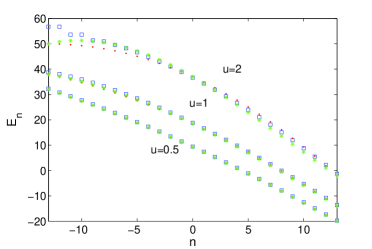
Figure 1: (Color online) The energy spectrum of the BH Hamiltonian for $J=1$ and $N=26$. The blue squares are obtained by numerical diagonalization of the Hamiltonian matrix for the Hamiltonian (3). The red dots are analytically calculated to the first order in $u$ (19) and the green stars are analytically calculated to the second order in $u$ (see (24)).

A natural question is what are the corrections to the leading order in the Semiclassical expansion presented here. In App. D it is shown that the correction is of order $\frac{1}{N^{2}}$. Hence it is of the form $\frac{1}{N^{2}}f\left(H\right)$. Then, this term should be added to the RHS of (21) leading to an additional correction to the energy levels. In App. D. we estimate this correction for representative values of the parameters and find it to be extremely small.

IV The pertubative calculation of the spectrum

It is possible to calculate the spectrum of (8) by using standard quantum perturbation theory for small $u$. The perturbation series is likely to converge if $uN<1$ since the energy differences are of order $\frac{1}{N}$, see (33). In the first order in $u$,

$$\widetilde{E}^{\left(1\right)}=-\frac{n}{N}+u\left\langle n\left|S_{z}^{2}\right|n\right\rangle.$$ (25)

The matrix element $\left\langle k\left|S_{z}^{2}\right|n\right\rangle$ can be calculated easily by using the relation

$$S_{z}=\frac{1}{2}\left(\widetilde{S}_{+}+\widetilde{S}_{-}\right)$$ (26)

where $\widetilde{S}_{\pm}=\left(S_{z}\mp iS_{y}\right)$ given by (4) are ladder operators satisfying

$$\widetilde{S}_{\pm}\left|n\right\rangle=\frac{1}{N}\sqrt{\left(\frac{N}{2}\pm n+1\right)\left(\frac{N}{2}\mp n\right)}\left|n\pm 1\right\rangle$$ (27)

$$\widetilde{S}_{\pm}\left|n\right\rangle=\frac{1}{2}\sqrt{1+\frac{2}{N}-\frac{4n^{2}}{N^{2}}\mp\frac{4n}{N^{2}}}\left|n\pm 1\right\rangle.$$ (28)

Hence,

$$\begin{array}[]{ccl}S_{z}^{2}\left|n\right\rangle&=&\frac{1}{4}\left(\widetilde{S}_{+}^{2}+\widetilde{S}_{-}^{2}+\widetilde{S}_{+}\widetilde{S}_{-}+\widetilde{S}_{-}\widetilde{S}_{+}\right)\left|n\right\rangle\\ &=&\frac{1}{16}\cdot\sqrt{\left(1+\frac{2}{N}-\frac{4n^{2}}{N^{2}}-\frac{4n}{N^{2}}\right)\cdot\left(1+\frac{2}{N}-\frac{4\left(n+1\right)^{2}}{N^{2}}-\frac{4\left(n+1\right)}{N^{2}}\right)}\left|n+2\right\rangle\\ &&+\frac{1}{16}\cdot\sqrt{\left(1+\frac{2}{N}-\frac{4n^{2}}{N^{2}}+\frac{4n}{N^{2}}\right)\cdot\left(1+\frac{2}{N}-\frac{4\left(n-1\right)^{2}}{N^{2}}+\frac{4\left(n-1\right)}{N^{2}}\right)}\left|n-2\right\rangle\\ &&+\frac{1}{16}\cdot\sqrt{\left(1+\frac{2}{N}-\frac{4n^{2}}{N^{2}}+\frac{4n}{N^{2}}\right)\cdot\left(1+\frac{2}{N}-\frac{4\left(n-1\right)^{2}}{N^{2}}-\frac{4\left(n-1\right)}{N^{2}}\right)}\left|n\right\rangle\\ &&+\frac{1}{16}\cdot\sqrt{\left(1+\frac{2}{N}-\frac{4n^{2}}{N^{2}}-\frac{4n}{N^{2}}\right)\cdot\left(1+\frac{2}{N}-\frac{4\left(n+1\right)^{2}}{N^{2}}+\frac{4\left(n+1\right)}{N^{2}}\right)}\left|n\right\rangle\end{array}.$$ (29)

Assuming $N\gg 1$, we expand $\left\langle n\left|S_{z}^{2}\right|n\right\rangle$ to the second order in $\frac{1}{N}$ and get

$$\begin{array}[]{ccl}\left\langle n\left|S_{z}^{2}\right|n\right\rangle&\approx&\frac{1}{16}\cdot\sqrt{1+\frac{4}{N}-\frac{8n^{2}}{N^{2}}+\frac{8n}{N^{2}}+\frac{4}{N^{2}}}\\ &&+\frac{1}{16}\cdot\sqrt{1+\frac{4}{N}-\frac{8n^{2}}{N^{2}}-\frac{8n}{N^{2}}+\frac{4}{N^{2}}}\\ &\approx&\frac{1}{16}\left[2+\frac{4}{N}-\frac{8n^{2}}{N^{2}}\right]\end{array}.$$ (30)

resulting in

$$\widetilde{E}^{\left(1\right)}=-\frac{n}{N}+\frac{u}{8}\left[1+\frac{2}{N}-\frac{4n^{2}}{N^{2}}\right],$$ (31)

which is equivalent to the semiclassical correction calculated in (18), if $\frac{1}{N}$ is ignored compared to $1$.

The energies to the second order in $u$ are

$$\widetilde{E}^{\left(2\right)}=-\frac{n}{N}+u\left\langle n\left|S_{z}^{2}\right|n\right\rangle+u^{2}\sum_{k\neq n}\frac{\left|\left\langle k\left|S_{z}^{2}\right|n\right\rangle\right|^{2}}{E_{n}^{\left(0\right)}-E_{k}^{\left(0\right)}}.$$ (32)

The energy differences are

$$\widetilde{E}_{n}^{\left(0\right)}-\widetilde{E}_{k}^{\left(0\right)}=\frac{k-n}{N}$$ (33)

and the matrix elements $\left\langle k\left|S_{z}^{2}\right|n\right\rangle$ does not vanish only for $k=n\pm 2$. Therefore,

$$\begin{array}[]{ccl}\sum_{k\neq n}\frac{\left|\left\langle k\left|S_{z}^{2}\right|n\right\rangle\right|^{2}}{E_{n}^{\left(0\right)}-E_{k}^{\left(0\right)}}&=&\frac{N}{2\cdot 16^{2}}\left(1+\frac{2}{N}-\frac{4n^{2}}{N^{2}}-\frac{4n}{N^{2}}\right)\cdot\left(1+\frac{2}{N}-\frac{4n^{2}}{N^{2}}-\frac{12n}{N^{2}}-\frac{8}{N^{2}}\right)\\ &&-\frac{N}{2\cdot 16^{2}}\left(1+\frac{2}{N}-\frac{4n^{2}}{N^{2}}+\frac{4n}{N^{2}}\right)\cdot\left(1+\frac{2}{N}-\frac{4n^{2}}{N^{2}}+\frac{12n}{N^{2}}-\frac{8}{N^{2}}\right)\\ &=&\frac{1}{16^{2}}\left[-\frac{4n}{N}\left(1+\frac{2}{N}-\frac{4\left(n^{2}+2\right)}{N^{2}}\right)-\frac{12n}{N}\left(1+\frac{2}{N}-\frac{4n^{2}}{N^{2}}\right)\right]\\ &=&-\frac{4n}{16^{2}N}\left[4+\frac{8}{N}-\frac{8}{N^{2}}-\frac{16n^{2}}{N^{2}}\right]=-\frac{n}{16N}\left[1+\frac{2}{N}-\frac{2}{N^{2}}-\frac{4n^{2}}{N^{2}}\right]\end{array}$$ (34)

and,

$$\widetilde{E}^{\left(2\right)}=-\frac{n}{N}+\frac{u}{8}\left[1+\frac{2}{N}-\frac{4n^{2}}{N^{2}}\right]+\frac{u^{2}}{16}\left[-\frac{n}{N}\left(1+\frac{2}{N}-\frac{2}{N^{2}}\right)+\frac{4n^{3}}{N^{3}}\right]$$ (35)

which is equivalent to the semiclassical correction calculated in (23), when $\frac{1}{N}$ is ignored compared to $1$.

V Dynamics

In this section, our aim is to derive an analytic expression for the expectation value of $S_{z}\left(t\right)$ that is the difference in occupation of the two sites where the initial condition is that all the bosons occupy the state $L$ and $\left\langle S_{z}\right\rangle=\frac{1}{2}$ (it is the north pole of the phase space Bloch sphere). In the framework of the BH model (3), it is possible to calculate $S_{z}\left(t\right)$ numerically Milburn . The resulting $S_{z}\left(t\right)$ is a series of collapses and revivals, superimposed on rapid oscillations. We would like to utilize the spectrum (24) in order to study analytically the dynamics in the Rabi regime $u<1$.

In absence of inter-particle interactions ($u=0$), the operator $S_{x}$ commutes with the Hamiltonian (8). Hence, for $u<1$, the eigenstates of (8) can be approximated by the eigenstates of $S_{x}$ (corrections of higher order will be discussed later), namely by

$$\left|n\right\rangle\equiv\frac{1}{\sqrt{\left(\frac{N}{2}+n\right)!\left(\frac{N}{2}-n\right)!}}\left(a_{+}^{\dagger}\right)^{\frac{N}{2}+n}\left(a_{-}^{\dagger}\right)^{\frac{N}{2}-n}\left|0\right\rangle.$$ (36)

where $a_{\pm}^{\dagger}=\frac{1}{\sqrt{2}}\left(a_{L}^{\dagger}\pm a_{R}^{\dagger}\right)$ and

$$\left[a_{+},a_{-}\right]=0$$ (37)

$$\left[a_{+},a_{+}^{\dagger}\right]=1$$ (38)

$$\left[a_{-},a_{-}^{\dagger}\right]=1$$ (39)

The reason for (36) is that

$$S_{x}=\frac{1}{2N}\left(a_{+}^{\dagger}a_{+}-a_{-}^{\dagger}a_{-}\right).$$ (40)

In what follows, we calculate the evolution of the operator

$$\widetilde{S}_{+}\equiv N\left(S_{z}-iS_{y}\right)=\frac{1}{2}\left(a_{L}^{\dagger}+a_{R}^{\dagger}\right)\left(a_{L}-a_{R}\right)=a_{+}^{\dagger}a_{-}$$ (41)

for the initial condition

$$\left|\psi\left(t=0\right)\right\rangle=\frac{1}{\sqrt{N!}}\left(a_{L}^{\dagger}\right)^{N}=\frac{1}{2^{N/2}\sqrt{N!}}\left(a_{+}^{\dagger}+a_{-}^{\dagger}\right)^{N}.$$ (42)

It is useful to expand $\left|\psi\left(t=0\right)\right\rangle$ in the basis of (36),

$$\left|\psi\left(t=0\right)\right\rangle=\sum_{n=-N/2}^{N/2}c_{n}\left|n\right\rangle,$$ (43)

where

$$c_{n}=\frac{1}{2^{N/2}\sqrt{N!}}\cdot\left(\begin{array}[]{c}N\\ \frac{N}{2}+n\end{array}\right)\cdot\sqrt{\left(\frac{N}{2}+n\right)!\left(\frac{N}{2}-n\right)!}=\frac{1}{2^{N/2}}\sqrt{\left(\begin{array}[]{c}N\\ \frac{N}{2}+n\end{array}\right)}.$$ (44)

For $N\gg 1$ and $n\ll\frac{N}{2}$, the binomial coefficients can be approximated by a Gaussian,

$$c_{n}\approx\left(\frac{2}{\pi N}\right)^{\frac{1}{4}}e^{-\frac{n^{2}}{N}}.$$ (45)

We note that the normalized difference between the occupation of the two sites is

$$\Delta\left(t\right)=\left\langle\psi\left|S_{z}\right|\psi\right\rangle=\frac{1}{N}\mathrm{Re}\left\langle\psi\left|\widetilde{S}_{+}\right|\psi\right\rangle$$ (46)

where $\widetilde{S}_{+}\equiv N\left(S_{z}-iS_{y}\right)=\frac{1}{2}\left(a_{L}^{\dagger}+a_{R}^{\dagger}\right)\left(a_{L}-a_{R}\right)=a_{+}^{\dagger}a_{-}$. In the basis $\left\{\left|n\right\rangle\right\}$, $\widetilde{S}_{+}$ is a raising operator, therefore,

$$\widetilde{S}_{+}\left|n\right\rangle=\sqrt{\left(\frac{N}{2}+n+1\right)\left(\frac{N}{2}-n\right)}\left|n+1\right\rangle,$$ (47)

we used (37), (38) and (39).The expectation value of $\widetilde{S}_{+}$ at time $t$ for the initial condition (43) is

$$\left\langle\psi\left(t\right)\left|\widetilde{S}_{+}\right|\psi\left(t\right)\right\rangle=\sum_{n=-N/2}^{N/2}\sqrt{\left(\frac{N}{2}+n+1\right)\left(\frac{N}{2}-n\right)}c_{n}c_{n+1}e^{-i\left(E_{n}^{\left(BH2\right)}-E_{n+1}^{\left(BH2\right)}\right)t}.$$ (48)

First, note that

$$c_{n}c_{n+1}=\frac{\sqrt{2}}{\sqrt{\pi N}}e^{-\frac{2n^{2}+2n+1}{N}}.$$ (49)

According to (24),

$$E_{n}^{\left(BH2\right)}-E_{n+1}^{\left(BH2\right)}=J\left(2+\frac{2}{N}un+\frac{1}{8}u^{2}-\frac{3}{2N^{2}}u^{2}n^{2}+\frac{u}{N}-\frac{3}{2N^{2}}u^{2}n-\frac{1}{2N^{2}}u^{2}\right).$$ (50)

Since $u<1$, we can neglect the term $\frac{3}{2N^{2}}u^{2}n$ which is much smaller than $\frac{2}{N}un$. For large $N$ and $n\ll\frac{N}{2}$, (48) can be written in the form

$$\left\langle\psi\left(t\right)\left|\widetilde{S}_{+}\right|\psi\left(t\right)\right\rangle=\frac{N}{2}\widetilde{S}e^{-i\phi t}$$ (51)

where

$$\phi=J\left(2+\frac{1}{8}u^{2}+\frac{u}{N}-\frac{1}{2N^{2}}u^{2}\right)$$ (52)

and

$$\widetilde{S}=\frac{\sqrt{2}}{\sqrt{\pi N}}\sum_{n=-N/2}^{N/2}e^{-\frac{2n^{2}+2n+1}{N}}e^{-i\frac{J}{N}\left(2un-\frac{3}{2N}u^{2}n^{2}-\frac{3}{2N}u^{2}n\right)t}.$$ (53)

We note that $e^{-i\phi t}$ is a rapidly oscillating function of $t$ with a period that is approximately $\frac{\pi}{J}$. We turn now to explore the envelope of $\widetilde{S}$. Since $n$ is an integer, in first order in $u$, the envelope of the sum (48) is a periodic function of $t$ with period (revival time) of

$$T_{R}=\frac{\pi N}{uJ}.$$ (54)

Actually $T_{R}$ is the inverse of the coefficient of the linear term in $n$ in the RHS of (50), namely $\frac{1}{T_{R}}=\frac{J}{2\pi}\left(\frac{2}{N}u+\frac{3u^{2}}{2N^{2}}\right)$. The estimate (54) assumes $\frac{u}{N}\ll 1$. The terms proportional to $u^{2}$ in (50) are ignored for the same reason, taking into account that in what follows only terms where $n\ll N$ are important. Around the $m$-th revival, we write $t=m\cdot T_{R}+\tau$ with $-\frac{1}{2}T_{R}<\tau<\frac{1}{2}T_{R}$ and write $\widetilde{S}=\sum_{m}\widetilde{S}_{m}$ where

$$\begin{array}[]{ccc}\widetilde{S}_{m}&=&\frac{\sqrt{2}}{\sqrt{\pi N}}\sum_{-\infty}^{\infty}e^{-\left(2n^{2}+2n+1\right)/N}e^{-i\frac{J}{N}\left(2un-\frac{3}{2N}u^{2}n^{2}\right)\cdot\left(m\cdot T_{R}+\tau\right)}\\ &=&\frac{\sqrt{2}}{\sqrt{\pi N}}\sum_{-\infty}^{\infty}e^{-\left(2n^{2}+2n+1\right)/N}e^{+i\frac{3}{2N^{2}}u^{2}n^{2}J\cdot\left(m\cdot T_{R}+\tau\right)-\frac{2}{N}iJun\tau}\end{array}.$$ (55)

We approximate the sum by an integral

$$\widetilde{S}_{m}\approx\frac{\sqrt{2}}{\sqrt{\pi N}}\int_{-\infty}^{\infty}e^{-\left(2n^{2}+2n+1\right)/N}e^{+i\frac{3}{2N^{2}}u^{2}n^{2}J\cdot\left(m\cdot T_{R}+\tau\right)-\frac{2}{N}iJun\tau}dn.$$ (56)

What enables to approximate the sum over $n$ by an integral is the fact that in the vicinity of a revival $\frac{J}{N}u\tau+\frac{3}{N^{2}}u^{2}n\tau$ is small (while $\frac{J}{N}unt$ is typically large). The integral was calculated in App. B (where we should take $\beta=\gamma=1$ and $\bar{m}=m$ for the calculations of the present section) using $\psi$ in the order $u^{0}$ and in App. C the corrections of the order $u$ and $u^{2}$ were added. In App. E it is verified that the semiclassical wave function gives the same result. The result is

$$\widetilde{S}_{m}=\frac{\sqrt{2}R}{D_{D}^{1/4}}e^{\frac{D_{R}}{D_{D}}-\frac{1}{N}+i\left(\phi_{s}+\phi^{\prime}_{s}\right)}$$ (57)

where $D_{R},D_{D}$ and $\phi_{s}$ are given by (98), (100), (106),

$$\frac{D_{R}}{D_{D}}\approx\frac{-2J^{2}u^{2}\left(\tau+\frac{3m\pi}{2J}\right)^{2}+2+\frac{9}{2}u^{2}m^{2}\pi^{2}}{N\left[4+\frac{9}{4}u^{2}\left(m\pi+\frac{J}{N}u\tau\right)^{2}\right]},$$ (58)

and $R$ and $\phi^{\prime}_{s}$ will be calculated in what follows.

$$R=\left|1+\frac{u}{4}\left(\frac{B}{A}-1\right)-\frac{u^{2}}{32}\right|\approx 1-\frac{u^{2}}{32}\approx e^{-\frac{u^{2}}{32}}$$ (59)

and

$$\tan\phi^{\prime}_{s}\approx\frac{u^{2}}{8}\left(2J\tau+\frac{3}{2}m\pi\right).$$ (60)

For small $u$, $\phi^{\prime}_{s}\approx\tan\phi^{\prime}_{s}\approx\frac{u^{2}}{8}\left(2J\tau+\frac{3}{2}m\pi\right)$.

The resulting $\widetilde{S}_{m}$ (57) is approximately a Gaussian of a width

$$\Delta t_{R}^{m}\approx\frac{\sqrt{2N\left(1+\frac{9}{16}u^{2}m^{2}\pi^{2}\right)}}{Ju}.$$ (61)

Therefore, $\tau\lesssim\frac{\sqrt{2N}}{Ju}$ and $\frac{J}{N}u\tau$ (see denominator on (58)) is of order $\frac{1}{\sqrt{N}}$ and can be neglected compared to $m\pi$, as was done in (61) and in the following equations.

For small $m$, $\Delta t_{R}^{m}\ll T_{R}$. However, there is an $m_{max}$ where the width $\Delta t_{R}^{m}$ is comparable to $T_{R}$ and then the revivals mix and our calculations are not valid. Defining $m_{max}$ by $\Delta t_{R}^{m_{max}}=\frac{1}{2}T_{R}$, we estimate

$$m_{max}=\frac{\sqrt{2\left(\pi^{2}N-8\right)}}{3u\pi},$$ (62)

namely, the revivals start to mix at time

$$T_{B}=m_{max}T_{R}\approx\frac{\pi\sqrt{2}N^{\frac{3}{2}}}{3u^{2}J}.$$ (63)

For times $t<m_{max}T_{R}$, in the leading order in $u$, $\widetilde{S}$ can be approximated by

$$\widetilde{S}=\sum_{m}\frac{e^{-\frac{u^{2}}{32}}}{\left[1+\frac{9}{16}u^{2}m^{2}\pi^{2}\right]^{1/4}}\exp\left[\frac{-\frac{1}{2}J^{2}u^{2}\left(t+\frac{3m\pi}{2J}-mT_{R}\right)^{2}+\eta}{N\left(1+\frac{9}{16}u^{2}m^{2}\pi^{2}\right)}+i\left(\phi_{s}+\phi^{\prime}_{s}\right)\right].$$ (64)

Therefore,

$$\left\langle\psi\left(t\right)\left|\widetilde{S}_{+}\right|\psi\left(t\right)\right\rangle=\frac{N}{2}\sum_{m}\frac{e^{-\frac{u^{2}}{32}}}{\left[1+\frac{9}{16}u^{2}m^{2}\pi^{2}\right]^{1/4}}\exp\left[\frac{-\frac{1}{2}J^{2}u^{2}\left(t+\frac{3m\pi}{2J}-mT_{R}\right)^{2}+\eta}{N\left(1+\frac{9}{16}u^{2}m^{2}\pi^{2}\right)}+i\left(\phi_{1}-\phi t\right)\right]$$ (65)

and (see (46))

$$\Delta\left(t\right)=\frac{1}{2}\sum_{m}\frac{e^{-\frac{u^{2}}{32}}}{\left[1+\frac{9}{16}u^{2}m^{2}\pi^{2}\right]^{1/4}}\exp\left[\frac{-\frac{1}{2}J^{2}u^{2}\left(t+\frac{3m\pi}{2J}-mT_{R}\right)^{2}+\eta}{N\left(1+\frac{9}{16}u^{2}m^{2}\pi^{2}\right)}\right]\cos\left(\phi_{1}-\phi t\right),$$ (66)

$$\left\langle\psi\left(t\right)\left|\widetilde{S}_{y}\right|\psi\left(t\right)\right\rangle=\frac{1}{2}\sum_{m}\frac{e^{-\frac{u^{2}}{32}}}{\left[1+\frac{9}{16}u^{2}m^{2}\pi^{2}\right]^{1/4}}\exp\left[\frac{-\frac{1}{2}J^{2}u^{2}\left(t+\frac{3m\pi}{2J}-mT_{R}\right)^{2}+\eta}{N\left(1+\frac{9}{16}u^{2}m^{2}\pi^{2}\right)}\right]\sin\left(\phi t-\phi_{1}\right).$$ (67)

where

$$\eta=\frac{1}{2}+\frac{9}{8}u^{2}m^{2}\pi^{2}$$ (68)

and

$$\phi\approx J\left(2+\frac{1}{8}u^{2}+\frac{u}{N}\right).$$ (69)

In the expression for $\phi$ we neglected $\frac{1}{N^{2}}$ compared to $1$ in (52). The other phase variable is

$$\phi_{1}=\phi_{s}+\phi^{\prime}_{s}\approx\frac{u^{2}}{8}\left(2J\tau+\frac{3}{2}m\pi\right)+u\left(\frac{J\tau}{N}+\frac{3}{8}\left(1+\frac{1}{N}\right)\left(m\cdot\pi+\frac{J}{N}u\tau\right)\right),$$ (70)

neglecting $\frac{1}{N}$ compared to $1$, one finds

$$\phi_{1}=\phi_{s}+\phi^{\prime}_{s}\approx\frac{u^{2}}{8}\left(2J\tau+\frac{3}{2}m\pi\right)+u\left(\frac{J\tau}{N}+\frac{3}{8}\left(m\cdot\pi+\frac{J}{N}u\tau\right)\right).$$ (71)

The evolution of the expectation of the normalized difference in occupation of the two sites is the main result of the present work. In Fig. 2 it is compared to exact results found by numerical diagonalization of the Hamiltonian (3), for $u=\frac{1}{2},N=100$ and $J=1$. In Fig. 2 as well as in Figs. 3 the expressions (69) and (71) for the phases were used. We checked that if (52) and (70) are used instead, the results cannot be distinguished in the plots. We note remarkable agreement of the envelope with the exact numerical result. The rapid oscillations, exhibit good agreement for short times (Fig. 2(c)) but it deteriorates for longer times (Fig. 2(d)).

In Fig. 3 the evolution of the difference in occupation between the two sites is presented for $u=\frac{1}{20},N=50$ and $J=1$. We note also the remarkable agreement between the analytical and numerical results found for the envelope. The prediction for the rapid oscillations agrees with the exact results for longer times and more revivals than in Fig. 2.

(a)                        (b)

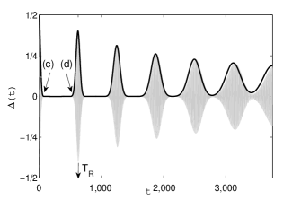
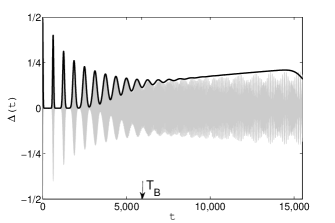
(c)                        (d)

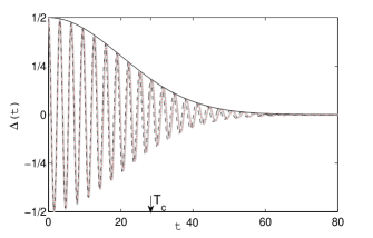
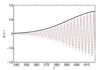
Figure 2: (Color online) The normalized difference between the occupation of the two sites $\Delta\left(t\right)$ for $J=1$, $N=100$ and $u=\frac{1}{2}$. The light gray line represents the numerical result, obtained by diagonalizing the Hamiltonian (2). The black line represents the envelope based on (66). (a) $\Delta\left(t\right)$ for the time regime $t<T_{B}$. The arrows show the time regimes which are presented in (c) and (d). The time $T_{R}$ of (54) is marked. (b) Long time blurring. The time $T_{B}$ where the revivals mix (see Eqs. (62) and (63)) is marked. (c) Short time dynamics. The red dashed-dot line is given by (66) where $\phi$ and $\phi_{1}$ are given by (69) and (71). The dashed black line presents oscillations with the unperturbed Rabi’s frequency $2J$ (that is approximating the phase $\phi t-\phi_{1}$ by $2Jt$) and $T_{c}$ of (75) is marked. (d) the same as (c) for a time interval near the revival $m=1$, where the analytical result for the phase $\phi_{1}-\phi t$ (66) no longer agrees with the result of exact numerical calculation.

(a)                        (b)

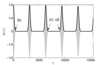
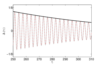
(c)                        (d)

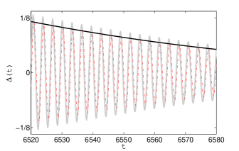
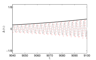
Figure 3: (Color online) Similar to Fig. 2 but for $J=1$, $N=50$ and $u=\frac{1}{20}$. (a)$\Delta\left(t\right)$ for a the time $t<T_{B}$. The arrows show the time regimes which are presented in (b)-(d). (b) Short time dynamics. (c) the same as (b) for a time interval near the revival $m=2$. (d) the same as (b) for a time interval near the revival $m=3$, where the analytical result for the phase of (66) no longer agrees with the exact numerical calculation.

For short times $\left(m=0\right)$, the dynamics is described by

$$\Delta\left(t\right)=\left\langle\psi\left|S_{z}\right|\psi\right\rangle=\frac{1}{2}e^{-\frac{1}{2N}J^{2}u^{2}t^{2}}\cos\left(\phi t-\phi_{1}\right)$$ (72)

and

$$\left\langle\psi\left(t\right)\left|S_{y}\right|\psi\left(t\right)\right\rangle=-\frac{1}{2}e^{-\frac{1}{2N}J^{2}u^{2}t^{2}}\sin\left(\phi t-\phi_{1}\right).$$ (73)

Both the expectations of $S_{z}$ and $S_{y}$ oscillate rapidly with the Rabi frequency $\frac{\pi}{J}$, and at the short time scale have a Gaussian envelope which is

$$f\left(t\right)=\frac{1}{2}e^{-\frac{1}{2N}J^{2}u^{2}t^{2}}$$ (74)

in the leading order in $u$ and $\frac{1}{N}$. Namely, it decays on the time scale

$$T_{c}=\frac{\sqrt{2N}}{Ju}.$$ (75)

Note that correction term $J\left(\frac{1}{8}u^{2}+\frac{u}{N}\right)$ to the phase in (69) improves the agreement with the exact numerical results compared to Rabi’s phase $2Jt$ (see Fig. 2c).

For $m>m_{max}$ the revival peaks overlap and the picture presented in Figs. 2a and 3a is blurred as demonstrated in Fig. 2b.

VI Initial conditions where both sites are occupied

It is interesting to study the dynamics of a double well where the initial condition is different occupation of the two wells. Such situation is encountered, for example, if a condensate is suddenly separated into two unequal parts, as was done in jeff . The initial condition is of the form

$$\left|\psi\left(t=0\right)\right\rangle=\frac{1}{\sqrt{N!}}\left(a_{R}^{\dagger}\cos\alpha+a_{L}^{\dagger}\sin\alpha\right)^{N}=\frac{1}{2^{N/2}\sqrt{N!}}\left[\left(\cos\alpha+\sin\alpha\right)a_{+}^{\dagger}+\left(\cos\alpha-\sin\alpha\right)a_{-}^{\dagger}\right]^{N}.$$ (76)

Expansion of (76) as a sum $\sum_{n=0}^{N}c_{n}\left|n\right\rangle$ (with $\left|n\right\rangle$ given by (36)) yields

$$\begin{array}[]{ccc}\left|c_{n}\right|&=&\frac{1}{2^{N/2}}\sqrt{\left(\begin{array}[]{c}N\\ \frac{N}{2}+n\end{array}\right)}\left[\left(\cos\alpha+\sin\alpha\right)^{\frac{N}{2}-n}\left(\cos\alpha-\sin\alpha\right)^{\frac{N}{2}+n}\right].\end{array}$$ (77)

The coefficients $c_{n}$ of substantial magnitude are distributed around

$$n_{max}=\frac{N}{2}\sin\left(2\alpha\right)$$ (78)

so that

$$c_{n}=\left(\frac{2\beta}{\pi N}\right)^{\frac{1}{4}}e^{-\frac{1}{N}\beta\left(n-n_{max}\right)^{2}}$$ (79)

and

$$c_{n}c_{n+1}=\sqrt{\frac{2\beta}{\pi N}}e^{-\frac{2}{N}\beta\left[\left(n-n_{max}\right)^{2}+\left(n-n_{max}\right)+\frac{1}{2}\right]}.$$ (80)

where

$$\beta=\frac{1}{\cos^{2}\left(2\alpha\right)}.$$ (81)

The expectation value $\Delta\left(t\right)=\left\langle S_{z}\left(t\right)\right\rangle$ is calculated in a similar way to what was done in the previous section. The differences are:

1. $\frac{n_{max}}{N}$ is not necessarily negligible and therefore $\widetilde{S}_{+}\left|n\right\rangle=\sqrt{\left(\frac{N}{2}+n+1\right)\left(\frac{N}{2}-n\right)}\left|n+1\right\rangle\approx\sqrt{\frac{N^{2}}{4}-n_{max}^{2}}\left|n+1\right\rangle$ and not $\frac{N}{2}\left|n+1\right\rangle$ (see for comparison (47)) .

2. Due to (80), $\Delta\left(t\right)=\left\langle S_{z}\left(t\right)\right\rangle$ is multiplied by $\sqrt{\beta}$.

3. The $\beta$ in the exponent of (80) affects the result of the integral $\widetilde{S}_{m}$ of (56), see App. B.

4. For $n\approx n_{max}$, it is possible that $\frac{3}{2N^{2}}u^{2}n^{2}$ in (50) is not negligible compared to $\frac{2}{N}un$. Consequently, the revival time $T_{R}$ will be modified as described in what follows. We substitute in (50) $n=n_{max}+\Delta n$ and write $E_{n}^{\left(BH2\right)}-E_{n+1}^{\left(BH2\right)}=J\left(2+\frac{2}{N}u\left(n_{max}+\Delta n\right)+\frac{1}{8}u^{2}-\frac{3}{2N^{2}}u^{2}\left(n_{max}+\Delta n\right)^{2}\right)$ for $n_{max}\gg 1$. The first constructive interference is obtained for $J\left(\frac{2}{N}u\Delta n-\frac{3}{N^{2}}u^{2}n_{max}\Delta n\right)T_{R}=2\pi$, namely

   $$T_{R}=\gamma\frac{\pi N}{uJ}$$ (82)

   where $\gamma=\left(1-\frac{3}{2}u\frac{n_{max}}{N}\right)^{-1}=\left(1-\frac{3}{4}u\sin\left(2\alpha\right)\right)^{-1}$.

Therefore, for the initial condition (76), the expectation value $\Delta\left(t\right)$ takes the form (as can be seen by modifying (66)),

$$\Delta\left(t\right) = \frac{\sqrt{\beta\left(\frac{N^{2}}{4}-n_{max}^{2}\right)}}{2}\cdot$$ (84)

$$\sum_{m}\frac{e^{-\frac{u^{2}}{32}}}{\left[\beta^{2}+\frac{9}{16}u^{2}m^{2}\gamma^{2}\pi^{2}\right]^{1/4}}\exp\left[\frac{-\frac{1}{2}J^{2}u^{2}\beta\left(t+\frac{3m\pi}{2J}-mT_{R}\right)^{2}+\bar{\eta}}{N\left(\beta^{2}+\frac{9}{16}u^{2}m^{2}\gamma^{2}\pi^{2}\right)}\right]\cos\left(\bar{\phi}_{1}-\phi t\right)$$

where

$$\bar{\eta}=\frac{\beta^{3}}{2}+\frac{9}{8}\beta u^{2}m^{2}\pi^{2},$$ (85)

$$\bar{\phi}_{1}\approx\frac{u^{2}}{8\beta}\left(2J\tau+\frac{3}{2}m\gamma\pi\right)+u\left(\frac{J\tau\beta^{2}}{N}+\frac{3}{8\beta}\left(m\gamma\pi+\frac{J}{N}u\tau\right)\right)$$ (86)

and $\phi$ is given by (69).

We turn now to estimate the conditions for the validity of the approximation (84). The width of the Gaussian (80) is $\sqrt{\frac{N}{\beta}},$ therefore it is required that

$$\frac{N}{2}-n_{max}>\sqrt{\frac{N}{\beta}},$$ (87)

therefore by (78),

$$\varepsilon_{1}\equiv\frac{1}{\sqrt{N}}\left(\frac{2}{1-\sin\left(2\alpha\right)}\right)\left|\cos\left(2\alpha\right)\right|<1.$$ (88)

The result (88) is demonstrated in Fig. 4.

In addition, the perturbation theory in $u$ adds to $\widetilde{S}_{m}$ a term of the form $\left(\frac{un_{max}}{N}\right)\widetilde{S}_{m}$ (see App. C (120), where the first order correction is calculated). Therefore, the higher orders can be neglected only if $un_{max}\ll N$, namely (see (78)),

$$\varepsilon_{2}\equiv\frac{un_{max}}{N}=\frac{u}{2}\sin\left(2\alpha\right)\ll 1.$$ (89)

Furthermore, the spectrum (24) is more accurate for small values of $\left|n\right|$ (see Fig. 1) where $H$ in (12) is small. If one wants to describe the dynamics for $\varepsilon_{2}\lesssim 1$, higher orders in the expansion of (12) might be needed.

(a)                        (b)

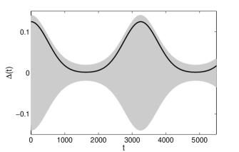
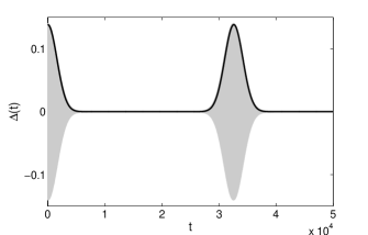
Figure 4: The normalized difference between the occupation of the two sites $\Delta\left(t\right)$ for the initial condition (76) with $\cos\alpha=\frac{3}{5}$, $\gamma=1.0373$. The parameters are $J=1$ and $u=\frac{1}{20}$, namely $\varepsilon_{2}=0.024$. The light gray line represents the exact numerical result, obtained by diagonalizing the Hamiltonian (3) and the black line represents the envelope based on (84). The numbers of particles are (a) $N=50$ (where $\varepsilon_{1}=14$) (b) $N=500$ (where $\varepsilon_{1}=0.63$).

VII Summary and discussion

In the present work the dynamics of the two site Bose Hubbard model defined by (2) and (3) were analyzed. We analyzed it for weak coupling $u$ (1) and for large number of particles $N$. The calculation was preformed to order $u^{2}$ and to the leading order in $\frac{1}{N}$, using a semiclassical method where $\frac{1}{N}$ plays the role of the Planck’s constant. It is important to note that this is not the standard quantum perturbation theory that requires $uN<O\left(1\right)$ but here it is requires only that $u\leq O\left(1\right)$.

In particular, the normalized difference in the occupation of the sites $\Delta\left(t\right)=\left\langle\psi\left(t\right)\left|S_{z}\right|\psi\left(t\right)\right\rangle$ as a function of time was calculated in a situation where initially all bosons are on one site leading to (66) with (68), (69) and (71). It is compared to the exact numerical solution in Figs. 2 and 3. For the envelope, remarkable agreement with the exact numerical solution is found. The solution exhibits rapid (Rabi) oscillations. The quality of the analytical result for these oscillations is initially very good but it deteriorates with time. The normalized population difference exhibits three time scales: $T_{c}$ (75), $T_{R}$ (54) and $T_{B}$ (63). Initially, it collapses at a time $T_{c}$ given by (75). Then, it exhibits revivals at times $mT_{R}$ with $T_{R}$ given by (54). These revivals are of increasing width (61). Eventually, at $T_{B}$ given by (63), this picture is washed away.

Comparison between the approximate result and the exact numerical calculation demonstrates that the result obtained indeed requires the terms in order $u^{2}$ and $\frac{1}{N}$. The classical approximation (10) reproduces correctly the rapid oscillations for short times. Such a behavior is found also for the GPE in double well Milburn ; Smerzi . Quantization is essential for the collapses and revivals. The collapse and revival times are predicted correctly by the first order in the interaction $u$, however for the width of the peaks the order $u^{2}$ is required, since the width depends on $m$ via the combination $m^{2}u^{2}$.

Collapses and revivals were found in various situations Milburn ; Bloch_colapse ; Lewenstein ; Wright ; wright&walls ; castin&dalibard ; Mark ; Talbot ; Berry&Sclich ; carpet ; Rayleigh ; Eberly . To the best of our knowledge, (66) is the only complete analytic description of this situation for a specific model of interacting bosons. It is reminiscent of the dynamics of the Jaynes-Cummings model Eberly .

We studied also the case where initially both sites are populated and found out an approximation that is good if the initial difference in occupation is sufficiently large. For finer details see Eqs. (88), (89) and Fig. 4. In this case, collapses and revivals are found as well where also here the collapse time $T_{c}$ and the width of the reviving peaks are proportional to $\sqrt{N}$ and the revival time is proportional to $N$. However, the revival time depends on the initial condition, as is seen from (82).

The generalization to other situations is left for further work.

Appendix A

In this appendix, we relate the BH Hamiltonian (3) to the spin Hamiltonian (5). Substituting the definitions (4) in (5), we get

$$H^{\prime}=-J\left(a_{R}^{\dagger}a_{L}+a_{R}^{\dagger}a_{L}\right)+\frac{U}{2}\left(a_{L}^{\dagger}a_{L}-a_{R}^{\dagger}a_{R}\right)^{2}.$$ (90)

The first term of $H^{\prime}$ is identical to the first term of $H_{BH}$. The second term is

$$\begin{array}[]{ccc}\frac{U}{2}\left(a_{L}^{\dagger}a_{L}-a_{R}^{\dagger}a_{R}\right)^{2}&=&\frac{U}{2}\left(a_{R}^{\dagger}a_{R}a_{R}^{\dagger}a_{R}-2a_{L}^{\dagger}a_{L}a_{R}^{\dagger}a_{R}+a_{L}^{\dagger}a_{L}a_{L}^{\dagger}a_{L}\right)\\ &=&\frac{U}{2}\left(a_{R}^{\dagger}a_{R}^{\dagger}a_{R}a_{R}+a_{R}^{\dagger}a_{R}-2a_{L}^{\dagger}a_{L}a_{R}^{\dagger}a_{R}+a_{L}^{\dagger}a_{L}^{\dagger}a_{L}a_{L}+a_{L}^{\dagger}a_{L}\right).\end{array}$$ (91)

We find that

$$\begin{array}[]{ccl}H_{BH}-H^{\prime}&=&\frac{U}{2}\left(a_{R}^{\dagger}a_{R}^{\dagger}a_{R}a_{R}-a_{R}^{\dagger}a_{R}+2a_{L}^{\dagger}a_{L}a_{R}^{\dagger}a_{R}+a_{L}^{\dagger}a_{L}^{\dagger}a_{L}a_{L}-a_{L}^{\dagger}a_{L}\right)\\ &=&\frac{U}{2}\left(a_{R}^{\dagger}a_{R}a_{R}^{\dagger}a_{R}+2a_{L}^{\dagger}a_{L}a_{R}^{\dagger}a_{R}+a_{L}^{\dagger}a_{L}a_{L}^{\dagger}a_{L}-2a_{R}^{\dagger}a_{R}-2a_{L}^{\dagger}a_{L}\right)\\ &=&\frac{1}{2}N^{2}U-NU.\end{array}$$ (92)

Therefore,

$$\begin{array}[]{ccc}H_{BH}&=&H^{\prime}+\frac{1}{2}JuN-Ju\end{array}.$$ (93)

That reduces to (5) up to a constant.

Appendix B

In this appendix, we calculate the integral (56) and the corresponding integral required in Sec. VI, which are of the form

$$\widetilde{S}^{\prime}{}_{m}=\int_{-\infty}^{\infty}e^{-\left(Ax^{2}+Bx\right)}dx=\sqrt{\frac{\pi}{A}}e^{B^{2}/4A}$$ (94)

where

$$\widetilde{S}{}_{m}=\frac{\sqrt{2}e^{-\frac{\beta}{N}}}{\sqrt{\pi N}}\widetilde{S}^{\prime}{}_{m}$$ (95)

$$\begin{array}[]{ccl}A&=\frac{1}{N}&\left[2\beta-\frac{3}{2}iu\left(\bar{m}\pi+\frac{J}{N}u\tau\right)\right]\\ B&=&\frac{2}{N}\left[\beta+iJu\tau\right]\\ \bar{m}&=&\gamma m.\end{array}$$ (96)

In Sec. V we consider the case $\beta=1,\gamma=1$ while in section VI, $\beta=\frac{1}{\cos^{2}\left(2\alpha\right)}$ and $\gamma=\left[1-\frac{3}{4}u\sin\left(2\alpha\right)\right]^{-1}$. There, $\alpha$ determines the initial conditions, see (76). In order to write (94) explicitly, we preform some manipulations where for each order of $\tau$, only the dominant order in $u$ is taken into account.

$$\frac{B^{2}}{4A}=\frac{\frac{1}{N}\left[\beta^{2}+2iJu\tau\beta-J^{2}u^{2}\tau^{2}\right]}{2\beta-\frac{3}{2}iu\left(\bar{m}\pi+\frac{J}{N}u\tau\right)}.$$ (97)

After multiplying the numerator and the denominator by the complex conjugate of the denominator,

$$\frac{B^{2}}{4A} = \frac{\left[\beta^{2}+2iJu\tau\beta-J^{2}u^{2}\tau^{2}\right]\left[2\beta+\frac{3}{2}iu\left(\bar{m}\pi+\frac{J}{N}u\tau\right)\right]}{N\left[4\beta^{2}+\frac{9}{4}u^{2}\left(\bar{m}\pi+\frac{J}{N}u\tau\right)^{2}\right]}$$

$$= \frac{2\beta^{3}+4iJu\tau\beta^{2}-2J^{2}u^{2}\tau^{2}\beta+\frac{3}{2}iu\beta^{2}\left(\bar{m}\pi+\frac{J}{N}u\tau\right)}{N\left[4\beta^{2}+\frac{9}{4}u^{2}\left(\bar{m}\pi+\frac{J}{N}u\tau\right)^{2}\right]}$$

$$-\frac{3Ju^{2}\tau\beta\left(\bar{m}\pi+\frac{J}{N}u\tau\right)+\frac{3}{2}iJ^{2}u^{3}\tau^{2}\left(\bar{m}\pi+\frac{J}{N}u\tau\right)}{N\left[4\beta^{2}+\frac{9}{4}u^{2}\left(\bar{m}\pi+\frac{J}{N}u\tau\right)^{2}\right]}$$

$$= \frac{2\beta^{3}-3Ju^{2}\tau\bar{m}\pi\beta-\beta\left(2J^{2}u^{2}+\frac{3}{N}J^{2}u^{3}\right)\tau^{2}}{N\left[4\beta^{2}+\frac{9}{4}u^{2}\left(\bar{m}\pi+\frac{J}{N}u\tau\right)^{2}\right]}$$

$$+\frac{i\left[4Ju\tau\beta^{2}+\frac{3}{2}u\beta^{2}\left(\bar{m}\pi+\frac{J}{N}u\tau\right)-\frac{3}{2}Ju^{3}\tau^{2}\left(\bar{m}\pi+\frac{J}{N}u\tau\right)\right]}{N\left[4\beta^{2}+\frac{9}{4}u^{2}\left(\bar{m}\pi+\frac{J}{N}u\tau\right)^{2}\right]}.$$

To the leading order in $u$,

$$\frac{B^{2}}{4A}=\frac{D_{R}+iD_{I}}{D_{D}}$$

where

$$D_{R}=\frac{1}{N}\left\{2\beta^{3}-3Ju^{2}\tau\bar{m}\pi\beta-2\beta J^{2}u^{2}\tau^{2}\right\}$$ (98)

$$D_{I}=\frac{1}{N}\left[4Ju\tau\beta^{2}+\frac{3}{2}u\beta^{2}\left(\bar{m}\pi+\frac{J}{N}u\tau\right)-\frac{3}{2}J^{2}u^{3}\tau^{2}\left(\bar{m}\pi+\frac{J}{N}u\tau\right)\right]$$ (99)

$$\begin{array}[]{ccl}D_{D}&=&4\beta^{2}+\frac{9}{4}u^{2}\left(\bar{m}\pi+\frac{J}{N}u\tau\right)^{2}\end{array}.$$ (100)

$D_{R}$ can be written as

$$D_{R}=-\frac{2\beta}{N}J^{2}u^{2}\left(\tau+\frac{3\bar{m}\pi}{2J}\right)^{2}+\frac{2\beta^{3}}{N}+\frac{9}{2N}u^{2}\bar{m}^{2}\pi^{2}\beta.$$ (101)

Now we turn to calculate $\sqrt{\frac{\pi}{A}}$ which appears in (94). According to (100),

$$A=\frac{\sqrt{D_{D}}}{N}e^{i\phi_{A}}$$ (102)

where

$$\tan\phi_{A}=-\frac{3}{4\beta}u\left(\bar{m}\cdot\pi+\frac{J}{N}u\tau\right).$$ (103)

Therefore,

$$\sqrt{\frac{\pi}{A}}=\frac{\sqrt{\pi N}}{D_{D}^{1/4}}e^{-i\frac{\phi_{A}}{2}}$$ (104)

and

$$\widetilde{S}_{m}=\frac{\sqrt{2}}{D_{D}^{1/4}}e^{\frac{D_{R}}{D_{D}}-\frac{\beta}{N}+i\phi_{S}}$$ (105)

where

$$\phi_{s}=\frac{D_{I}}{D_{D}}-\frac{\phi_{A}}{2}.$$ (106)

To the order $u^{2}$,

$$\phi_{A}\approx-\frac{3}{4\beta}u\left(\bar{m}\cdot\pi+\frac{J}{N}u\tau\right)$$ (107)

and

$$\phi_{s}=u\left(\frac{J\tau}{N}+\frac{3}{8}\left(\frac{1}{\beta}+\frac{1}{N}\right)\left(\bar{m}\cdot\pi+\frac{J}{N}u\tau\right)\right).$$ (108)

Appendix C

In this appendix we calculate the correction resulting from the fact that for $u\neq 0$ the eigenstates of $H=-S_{x}+uS_{z}^{2}$ are not identical to the eigenstates of $S_{x}$. Perturbation theory is justified only for $uN<1$ because the typical spacing between eigenvalues of $S_{x}$ is about $\frac{1}{N}$ while the maximum of the perturbation $uS_{z}^{2}$ is about $\frac{u}{4}$. However, most of the results presented in Sec. V-VI are applicable for $u<1$ (where it is possible that $uN\gg 1$). This is understood in the framework of some aspect of restricted quantum-classical correspondence Doron_cp1 ; doron_cp2 ; Doron_cp3 ; Doron_cp4 . Let us denote the corrected eigenstates of $H$ by $\left|n^{\prime}\right\rangle$. To the first order in $u$,

$$\left|n\right\rangle^{\prime}=\left|n\right\rangle+u\sum_{k\neq n}\left|k\right\rangle\cdot\frac{\left\langle k\left|S_{z}^{2}\right|n\right\rangle}{E_{n}-E_{k}}.$$ (109)

The matrix element $\left\langle k\left|S_{z}^{2}\right|n\right\rangle$ can be calculated easily by using (29) up to the second order in $\frac{1}{N}$. The result is

$$\left\langle k\left|S_{z}^{2}\right|n\right\rangle\approx\frac{1}{16}\left[d_{2}\left(n\right)\delta_{k,n+2}+d_{-2}\left(n\right)\delta_{k,n-2}+d_{0}\left(n\right)\delta_{k,n}\right]$$ (110)

where

$$d_{2}\left(n\right) = 1-\frac{4\left(n+1\right)^{2}}{N^{2}}+\frac{2}{N}$$

$$d_{-2}\left(n\right) = 1-\frac{4\left(n-1\right)^{2}}{N^{2}}+\frac{2}{N}$$ (111)

$$d_{0}\left(n\right) = 2+\frac{4}{N}-\frac{8n^{2}}{N^{2}}.$$

The energy difference is (33) and therefore

$$\left|n\right\rangle^{\prime}=\left|n\right\rangle+\frac{uN}{32}\left[d_{2}\left(n\right)\left|n+2\right\rangle-d_{-2}\left(n\right)\left|n-2\right\rangle\right].$$ (112)

For small $n$ and $u$ relevant for the present work, it agrees with the semiclassical result (160). We would like to expand the wavefunction in basis $\left|n\right\rangle^{\prime}$. For this purpose, we define the expansion coefficients

$$c^{\prime}_{n}=\sum_{k}c_{k}\left\langle k|n\right\rangle.$$ (113)

According to (112),

$$\begin{array}[]{ccl}c^{\prime}_{n}&\approx&c_{n}+\frac{uN}{32}\left[d_{2}\left(n\right)c_{n+2}-d_{-2}\left(n\right)c_{n-2}\right]\end{array}$$ (114)

while the coefficients $c_{n}$ are given by (79) ($\beta$ and $n_{max}$ are defined by (81) and (78), in Sec. V, $\beta=1$ and $n_{max}=0$, resulting in (45)). Therefore,

$$c^{\prime}_{n}=\left(\frac{2\beta}{\pi N}\right)^{\frac{1}{4}}e^{-\frac{1}{N}\beta\left(n-n_{max}\right)^{2}}\left[1+\frac{uN}{32}d_{2}\left(n\right)e^{-\frac{4}{N}\beta\left(n-n_{max}+1\right)}-\frac{uN}{32}d_{-2}\left(n\right)e^{+\frac{4}{N}\beta\left(n-n_{max}-1\right)}\right].$$ (115)

In the leading order in $\frac{1}{N}$, $\frac{n}{N}\approx\frac{n_{max}}{N}$ and

$$c^{\prime}_{n}=\left(\frac{2\beta}{\pi N}\right)^{\frac{1}{4}}e^{-\frac{1}{N}\beta\left(n-n_{max}\right)^{2}}\left\{1-\frac{u}{4}\left[\beta\left(1-\frac{4n_{max}^{2}}{N^{2}}\right)\left(n-n_{max}\right)+2\frac{n_{max}}{N}\right]\right\},$$ (116)

and in the first order in $u$,

$$c^{\prime}_{n}c^{\prime}_{n+1}\approx\frac{\sqrt{2\beta}}{\sqrt{\pi N}}e^{-\frac{2\beta}{N}\left[\left(n-n_{max}\right)^{2}+\left(n-n{}_{max}\right)+\frac{1}{2}\right]}\left\{1-\frac{u}{2}\left[\beta\left(1-\frac{4n_{max}^{2}}{N^{2}}\right)\left(n-n_{max}+\frac{1}{2}\right)+2\frac{n_{max}}{N}\right]\right\}.$$ (117)

The resulting correction to $\widetilde{S}_{m}$ is a of the form

$$\widetilde{S}{}_{m}^{\left(1\right)}=-\frac{\sqrt{2\beta}e^{-\frac{\beta}{N}}}{\sqrt{\pi N}}\cdot\frac{u}{2}\beta\left(1-\frac{4n_{max}^{2}}{N^{2}}\right)\int_{-\infty}^{\infty}xe^{-\left(Ax^{2}+Bx\right)}dx-\frac{u}{2}\left[2\frac{n_{max}}{N}+\frac{\beta}{2}\left(1-\frac{4n_{max}^{2}}{N^{2}}\right)\right]\widetilde{S}{}_{m}$$ (118)

where $A,B$ are presented explicitly in App. B, Eq. (96) and $x=n-n_{max}$. The integral can be solved by using

$$\int_{-\infty}^{\infty}xe^{-\left(Ax^{2}+Bx\right)}dx = \frac{-B}{2A}e^{\frac{B^{2}}{4A}}\sqrt{\frac{\pi}{A}}$$ (119)

Therefore,

$$\widetilde{S}{}_{m}^{\left(1\right)}=-\frac{u}{2}\left[\beta\left(1-\frac{4n_{max}^{2}}{N^{2}}\right)\left(\frac{1}{2}-\frac{B}{2A}\right)+2\frac{n_{max}}{N}\right]\widetilde{S}{}_{m}.$$ (120)

Since $A$ and $B$ are of the same order of magnitude (see (59) and (60)), this correction is typically small if $\frac{un_{max}}{N}$ is small. For the case $n_{max}=0$ discussed in Sec. V, $\widetilde{S}{}_{m}^{\left(1\right)}$ is negligible. However, in other cases (discussed in Sec. VI) it might be important and then our approximation fails.

Now we calculate the second order correction for the case $\beta=1,\,n_{max}=0$ relevant for Sec. V.

$$\left|n\right\rangle^{\prime} = \left|n\right\rangle+u\sum_{k\neq n}\left|k\right\rangle\cdot\frac{\left\langle k\left|S_{z}^{2}\right|n\right\rangle}{E_{n}-E_{k}}+u^{2}\sum_{l,k\neq n}\left|k\right\rangle\cdot\frac{\left\langle k\left|S_{z}^{2}\right|l\right\rangle\left\langle l\left|S_{z}^{2}\right|n\right\rangle}{\left(E_{n}-E_{k}\right)\left(E_{n}-E_{l}\right)}$$ (121)

$$-u^{2}\sum_{k\neq n}\left|k\right\rangle\cdot\frac{\left\langle n\left|S_{z}^{2}\right|n\right\rangle\left\langle k\left|S_{z}^{2}\right|n\right\rangle}{\left(E_{n}-E_{k}\right)^{2}}-\frac{1}{2}u^{2}\left|n\right\rangle\cdot\sum_{k\neq n}\frac{\left\langle n\left|S_{z}^{2}\right|k\right\rangle\left\langle k\left|S_{z}^{2}\right|n\right\rangle}{\left(E_{n}-E_{k}\right)^{2}}.$$

According to (110),

$$\left|n\right\rangle^{\prime} = \left|n\right\rangle+\frac{uN}{32}\left[d_{2}\left(n\right)\left|n+2\right\rangle-d_{-2}\left(n\right)\left|n-2\right\rangle\right]$$

$$+\frac{u^{2}N^{2}}{8\cdot 16^{2}}\left[d_{2}\left(n\right)d_{2}\left(n+2\right)\left|n+4\right\rangle+d_{-2}\left(n\right)d_{-2}\left(n-2\right)\left|n-4\right\rangle\right]$$

$$+\frac{u^{2}N^{2}}{4\cdot 16^{2}}\left[d_{2}\left(n\right)d_{0}\left(n+2\right)\left|n+2\right\rangle+d_{-2}\left(n\right)d_{0}\left(n-2\right)\left|n-2\right\rangle\right]$$

$$-\frac{u^{2}N^{2}}{4\cdot 16^{2}}\left[d_{0}\left(n\right)d_{2}\left(n\right)\left|n+2\right\rangle+d_{0}\left(n\right)d_{-2}\left(n\right)\left|n-2\right\rangle\right]$$

$$-\frac{u^{2}N^{2}}{8\cdot 16^{2}}\left(d_{2}\left(n\right)d_{-2}\left(n+2\right)+d_{-2}\left(n\right)d_{2}\left(n-2\right)\right)\left|n\right\rangle$$

$$= \left|n\right\rangle+\frac{uN}{32}\left[d_{2}\left(n\right)\left|n+2\right\rangle-d_{-2}\left(n\right)\left|n-2\right\rangle\right]$$

$$+\frac{u^{2}N^{2}}{8\cdot 16^{2}}\left[d_{2}\left(n\right)d_{2}\left(n+2\right)\left|n+4\right\rangle+d_{-2}\left(n\right)d_{-2}\left(n-2\right)\left|n-4\right\rangle\right]$$

$$+\frac{u^{2}N^{2}}{4\cdot 16^{2}}\left\{\left[d_{2}\left(n\right)\left(d_{0}\left(n+2\right)-d_{0}\left(n\right)\right)\right]\left|n+2\right\rangle+\left[d_{-2}\left(n\right)\left(d_{0}\left(n-2\right)-d_{0}\left(n\right)\right)\right]\left|n-2\right\rangle\right\}$$

$$-\frac{u^{2}N^{2}}{8\cdot 16^{2}}\left(d_{2}\left(n\right)d_{-2}\left(n+2\right)+d_{-2}\left(n\right)d_{2}\left(n-2\right)\right)\left|n\right\rangle.$$

namely,

$$\left|n\right\rangle^{\prime} \approx \left|n\right\rangle+\frac{uN}{32}\left[\left(1-\frac{4\left(n+1\right)^{2}}{N^{2}}+\frac{2}{N}\right)\left|n+2\right\rangle-\left(1-\frac{4\left(n-1\right)^{2}}{N^{2}}+\frac{2}{N}\right)\left|n-2\right\rangle\right]$$

$$+\frac{u^{2}N^{2}}{8\cdot 16^{2}}\left(1-\frac{4\left(n+1\right)^{2}}{N^{2}}-\frac{4\left(n+3\right)^{2}}{N^{2}}+\frac{4}{N}+\frac{4}{N^{2}}\right)\left|n+4\right\rangle$$

$$+\frac{u^{2}N^{2}}{8\cdot 16^{2}}\left(1-\frac{4\left(n-1\right)^{2}}{N^{2}}-\frac{4\left(n-3\right)^{2}}{N^{2}}+\frac{4}{N}+\frac{4}{N^{2}}\right)\left|n-4\right\rangle$$

$$-\frac{u^{2}N^{2}}{4\cdot 16^{2}}\left\{\frac{32\left(n+1\right)}{N^{2}}\left|n+2\right\rangle-\frac{32\left(n-1\right)}{N^{2}}\left|n-2\right\rangle\right\}$$

$$-\frac{u^{2}N^{2}}{4\cdot 16^{2}}\left(1-\frac{8\left(n^{2}+1\right)}{N^{2}}+\frac{4}{N}+\frac{4}{N^{2}}\right)\left|n\right\rangle.$$

Therefore,

$$c_{n}^{\prime} \approx \left(1-\frac{u^{2}N^{2}}{4\cdot 16^{2}}\left(1-\frac{8\left(n^{2}+1\right)}{N^{2}}+\frac{4}{N}+\frac{4}{N^{2}}\right)\right)c_{n}$$

$$+\frac{uN}{32}\left[\left(1-\frac{4\left(n+1\right)^{2}}{N^{2}}+\frac{2}{N}\right)c_{n+2}-\left(1-\frac{4\left(n-1\right)^{2}}{N^{2}}+\frac{2}{N}\right)c_{n-2}\right]$$

$$+\frac{u^{2}N^{2}}{8\cdot 16^{2}}\left(1-\frac{4\left(n+1\right)^{2}}{N^{2}}-\frac{4\left(n+3\right)^{2}}{N^{2}}+\frac{4}{N}+\frac{4}{N^{2}}\right)c_{n+4}$$

$$+\frac{u^{2}N^{2}}{8\cdot 16^{2}}\left(1-\frac{4\left(n-1\right)^{2}}{N^{2}}-\frac{4\left(n-3\right)^{2}}{N^{2}}+\frac{4}{N}+\frac{4}{N^{2}}\right)c_{n-4}$$

$$-\frac{u^{2}N^{2}}{4\cdot 16^{2}}\left[\frac{32\left(n+1\right)}{N^{2}}c_{n+2}-\frac{32\left(n-1\right)}{N^{2}}c_{n-2}\right]$$

$$= \left(\frac{2}{\pi N}\right)^{\frac{1}{4}}e^{-\frac{n^{2}}{N}}\left\{1+\frac{uN}{32}\left[\left(1-\frac{4\left(n+1\right)^{2}}{N^{2}}+\frac{2}{N}\right)e^{-\frac{4n+4}{N}}-\left(1-\frac{4\left(n-1\right)^{2}}{N^{2}}+\frac{2}{N}\right)e^{\frac{4n-4}{N}}\right]\right.$$

$$+\frac{u^{2}N^{2}}{8\cdot 16^{2}}\left(1-\frac{4\left(n+1\right)^{2}}{N^{2}}-\frac{4\left(n+3\right)^{2}}{N^{2}}+\frac{4}{N}+\frac{4}{N^{2}}\right)e^{-\frac{8n+16}{N}}$$

$$+\frac{u^{2}N^{2}}{8\cdot 16^{2}}\left(1-\frac{4\left(n-1\right)^{2}}{N^{2}}-\frac{4\left(n-3\right)^{2}}{N^{2}}+\frac{4}{N}+\frac{4}{N^{2}}\right)e^{\frac{8n-16}{N}}$$

$$\left.-\frac{u^{2}N^{2}}{4\cdot 16^{2}}\left[\frac{32\left(n+1\right)}{N^{2}}e^{-\frac{4n+4}{N}}-\frac{32\left(n-1\right)}{N^{2}}e^{\frac{4n-4}{N}}\right]-\frac{u^{2}N^{2}}{4\cdot 16^{2}}\left(1-\frac{8\left(n^{2}+1\right)}{N^{2}}+\frac{4}{N}+\frac{4}{N^{2}}\right)\right\}.$$

Expending the exponent to the second order in $\frac{1}{N}$ yields

$$c_{n}^{\prime} \approx \left(\frac{2}{\pi N}\right)^{\frac{1}{4}}e^{-\frac{n^{2}}{N}}\left\{1-\frac{u^{2}N^{2}}{4\cdot 16^{2}}\left(1-\frac{8\left(n^{2}+1\right)}{N^{2}}+\frac{4}{N}+\frac{4}{N^{2}}\right)-\frac{un}{4}\right.$$

$$+\frac{u^{2}N^{2}}{4\cdot 16^{2}}\left[1-\frac{12}{N}+\frac{24n^{2}+28}{N^{2}}\right]$$

$$\left.-\frac{u^{2}N^{2}}{2\cdot 16}\cdot\frac{2}{N^{2}}\right\}$$

$$= \left(\frac{2}{\pi N}\right)^{\frac{1}{4}}e^{-\frac{n^{2}}{N}}\left\{1-\frac{un}{4}+\frac{u^{2}N}{4\cdot 16}\left[-1+\frac{2n^{2}-2}{N}\right]\right\}$$

and

$$c_{n}^{\prime}c_{n+1}^{\prime} \approx \frac{\sqrt{2}}{\sqrt{\pi N}}e^{-\frac{2n^{2}+2n+1}{N}}\left[1-\frac{u}{2}\left(n+\frac{1}{2}\right)\right.$$

$$\left.+\frac{u^{2}}{32}\left(-N+2n^{2}+2n+2n\left(n+1\right)\right)\right].$$

The second order correction to $\widetilde{S}_{m}$ is of the form

$$\widetilde{S}_{m}^{\left(2\right)} \approx- \frac{u^{2}N}{32}\widetilde{S}_{m}+\frac{\sqrt{2}}{\sqrt{\pi N}}\cdot\frac{u^{2}}{8}\int\left(x^{2}e^{-\left(Ax^{2}+Bx\right)}+xe^{-\left(Ax^{2}+Bx\right)}\right)dx$$ (131)

where $A$,$B$ are defined in (96). The integral can be calculated by using (119) and

$$\int_{-\infty}^{\infty}x^{2}e^{-\left(Ax^{2}+Bx\right)}dx=\frac{1}{2A}e^{\frac{B^{2}}{4A}}\cdot\sqrt{\frac{\pi}{A}}.$$ (132)

Therefore,

$$\widetilde{S}_{m}^{\left(2\right)} \approx -\frac{u^{2}N}{32}\widetilde{S}_{m}+\widetilde{S}_{m}\cdot\frac{u^{2}}{16A}\cdot\left(1-\frac{B}{2}\right)$$ (133)

$$\approx -\frac{u^{2}N}{32}\widetilde{S}_{m}+\widetilde{S}_{m}\cdot\frac{u^{2}N}{32}.\left(1-\frac{1}{N}\right)$$ (134)

$$\approx- \frac{u^{2}}{32}\widetilde{S}_{m}$$ (135)

and it is a small correction.

Appendix D

In this appendix we calculate higher orders of the WKB expansion and show that its contribution to the spectrum is not important. In the WKB expansion Tabor , one makes the ansatz

$$\psi\propto e^{iS\left(\varphi\right)/\hbar}$$ (136)

where $S\left(\varphi\right)$ is the series

$$S\left(\varphi\right)=S_{0}\left(\varphi\right)+\hbar S_{1}\left(\varphi\right)+\hbar^{2}S_{2}\left(\varphi\right)+\ldots$$ (137)

and

$$\frac{\partial S_{0}}{\partial\varphi} = S_{x}$$ (138)

$$S_{1}=\frac{1}{2}\ln S_{x}$$ (139)

$$\frac{\partial S_{2}}{\partial\varphi}=\frac{-1}{2\left(\frac{\partial S_{0}}{\partial\varphi}\right)}\left[\frac{\partial^{2}S_{1}}{\partial\varphi^{2}}+\left(\frac{\partial S_{1}}{\partial\varphi}\right)^{2}\right].$$ (140)

Here, $\hbar=\frac{1}{N}$. In Sec. III, we used the Bohr-Sommerfeld quantization, namely, we demanded $S\left(\varphi\right)=S\left(\varphi+2\pi\right)+2\pi n\hbar$ in order to find the spectrum. In the present work, $\hbar=\frac{1}{N}$ is understood. There, we replaced $S$ by $S_{0}$ which is justified only in the leading order in $\hbar.$ Finally, it turned out that the spectrum contains terms of higher orders of $\hbar$ (21)-(24) and therefore, the effects of $S_{1}$ and $S_{2}$ should be taken into account as well. Fortunately, the contributions of $S_{1}$ and $S_{2}$ are negligible as described in what follows. $S_{x}$ is periodic in $\varphi$ so that $S_{1}$ does not contribute to the spectrum.

In order to find the contribution of $S_{2}$, we first calculate the derivatives of $S_{1}$:

$$\frac{\partial S_{1}}{\partial\varphi}=\frac{1}{2S_{x}}\frac{\partial S_{x}}{\partial\varphi}$$ (141)

and

$$\frac{\partial^{2}S_{1}}{\partial\varphi^{2}}=\frac{-1}{2S_{x}^{2}}\left(\frac{\partial S_{x}}{\partial\varphi}\right)^{2}+\frac{1}{2S_{x}}\frac{\partial^{2}S_{x}}{\partial\varphi^{2}}.$$ (142)

Hence,

$$\frac{\partial S_{2}}{\partial\varphi}=\frac{-1}{4S_{x}^{2}}\left[\frac{-1}{2S_{x}}\left(\frac{\partial S_{x}}{\partial\varphi}\right)^{2}+\frac{\partial^{2}S_{x}}{\partial\varphi^{2}}\right].$$ (143)

In what follows, all calculations are performed to the order $\hbar^{2}$. We substitute $S_{x}$ of (20) and find

$$\frac{\partial S_{x}}{\partial\varphi}=\left(\frac{1}{4}-H^{2}\right)\left[u\sin\left(2\varphi\right)+8u^{2}H\sin^{3}\varphi\cos\varphi\right],$$ (144)

and

$$\frac{\partial^{2}S_{x}}{\partial\varphi^{2}}=\left(\frac{1}{4}-H^{2}\right)\left[2u\cos\left(2\varphi\right)+8u^{2}H\left(3\sin^{2}\varphi\cos^{2}\varphi-\sin^{4}\varphi\right)\right].$$ (145)

Therefore, to the second order in $u$,

$$\frac{\partial S_{2}}{\partial\varphi}=\frac{-1}{4S_{x}^{2}}\left(\frac{1}{4}-H^{2}\right)\left[\frac{-u^{2}}{2S_{x}}\left(\frac{1}{4}-H^{2}\right)\sin^{2}\left(2\varphi\right)+2u\cos\left(2\varphi\right)+8u^{2}H\left(3\sin^{2}\varphi\cos^{2}\varphi-\sin^{4}\varphi\right)\right].$$ (146)

Assuming $u\ll H$ we find $\frac{1}{S_{x}^{2}}\approx\frac{1}{H^{2}}\left(1+\frac{2}{H}u\left(\frac{1}{4}-H^{2}\right)\sin^{2}\varphi\right)$, leading to

$$\frac{\partial S_{2}}{\partial\varphi} = \frac{-1}{4H^{2}}\left(\frac{1}{4}-H^{2}\right)\left[\frac{u^{2}}{2H}\left(\frac{1}{4}-H^{2}\right)\left(\sin^{2}\left(2\varphi\right)+8\cos\left(2\varphi\right)\sin^{2}\varphi\right)\right.$$ (148)

$$\left.+2u\cos\left(2\varphi\right)+8u^{2}H\left(3\sin^{2}\varphi\cos^{2}\varphi-\sin^{4}\varphi\right)\right].$$

Therefore,

$$\bar{\delta}=\frac{\hbar^{2}}{2\pi}\left(S_{2}\left(\varphi+2\pi\right)-S_{2}\left(\varphi\right)\right)=\frac{-3u^{2}}{16H^{3}N^{2}}\left(\frac{1}{4}-H^{2}\right)^{2}.$$ (149)

This should be added to the right hand side of (21), resulting in a contribution of

$$\delta^{\prime}=\frac{3u^{2}N}{16n^{3}}\left(\frac{1}{4}-\frac{n^{2}}{N^{2}}\right)^{2}$$ (150)

to the spectrum (23). The approximation leading to this term is not valid for small $n$ (see (18) where $H$ is of order $u$). To find an estimate for the correction in this regime we repeat the calculation for $I=0$. If $n=0$,

$$\begin{array}[]{ccl}S_{x}&\approx&-\frac{u}{8}+\frac{1}{4}u\sin^{2}\varphi\end{array}$$ (151)

and the derivatives are $\frac{\partial S_{x}}{\partial\varphi}=\frac{1}{4}u\sin\left(2\varphi\right),$ $\frac{\partial^{2}S_{x}}{\partial\varphi^{2}}=\frac{1}{2}u\cos\left(2\varphi\right)$. Therefore, to the second order in $u$,

$$\frac{\partial S_{2}}{\partial\varphi} = \frac{-1}{4u\left(-\frac{1}{8}+\frac{1}{4}\sin^{2}\varphi\right)^{2}}\left[\frac{-1}{2\left(-\frac{1}{8}+\frac{1}{4}\sin^{2}\varphi\right)}\left(\frac{1}{4}\sin\left(2\varphi\right)\right)^{2}+\frac{1}{2}\cos\left(2\varphi\right)\right]$$ (152)

$$= \frac{4}{u\cos^{3}\left(2\varphi\right)}\left[\sin^{2}\left(2\varphi\right)-2\cos^{2}\left(2\varphi\right)\right].$$ (153)

This expression is antisymmetric with respect to $2\varphi=\frac{\pi}{2}+\alpha\rightarrow 2\varphi=\frac{\pi}{2}-\alpha$. Therefore the integral for $S_{2}$ vanishes. The above estimates are only for part of the spectrum. Therefore, we turn to a numerical estimate.

In Fig. 5, we present the numerically calculated deviations in the spectrum originating of $S_{2}$ and show that it is small for the parameters of Figs. 2-3. The calculation of the spectrum presented in Fig. 5 was carried out by iterations as described in what follows:

1. For each $n$, $S_{x}\left(\varphi\right)$ was calculated according to (12) where $H$ is replaced by the spectrum $E_{n}^{\left(2\right)}$ of (23).

2. $S_{2}\left(\varphi\right)$ was found by substitution of $S_{x}$ in (143) and integration over $\varphi$.

3. The term $\frac{\hbar^{2}}{2\pi}\left(S_{2}\left(\varphi+2\pi\right)-S_{2}\left(\varphi\right)\right)$ was added to the RHS of (21), which we solved numerically to obtain a corrected spectrum $\widetilde{E}{}_{n}^{\left(2\right)}$.

4. We repeated steps 1-3 where $H$ in $S_{x}$ is replaced by $\widetilde{E}{}_{n}^{\left(2\right)}$ until conversion.

5. We Multiplied the resulting spectrum by $2JN$ and added the constant $C_{N}$ to be able to compare with the exact BH spectrum.

(a)                        (b)

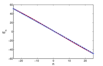
Figure 5: (Color online) Spectrum of the BH Hamiltonian, The red lines represent the spectrum (24) that was used in the calculation of the dynamics and the blue stars represent the spectrum which was obtained numerically by taking into account contributions up to order $\hbar^{2}$ in the semiclassical approximation, as described in the text. The exact spectrum of the BH Hamiltonian (obtained by diagonalization (3)) appears in black dashed line. (a) $J=1$, $N=100$ and $u=\frac{1}{2}$. (b) $J=1$, $N=50$ and $u=\frac{1}{20}$.

Appendix E

In this appendix, we calculate the eigenstates in the semiclassical approximation

$$\left|n^{\prime}\right\rangle=\frac{1}{\sqrt{2\pi}}e^{iS_{0}\left(\varphi\right)/\hbar}$$ (154)

and show that it can be approximated by the eigenstates of $S_{x}$ as was done in Sec. V and VI. According to (138) and (13), in the first order in $u$,

$$S_{0}=\frac{k}{N}\varphi-\frac{u}{4}\left[\frac{1}{4}-\frac{k{}^{2}}{N^{2}}\right]\sin\left(2\varphi\right).$$ (155)

The eigenstates of $S_{x}$ (obtained by substituting (155) with $u=0$ in (154)) are $e^{in\varphi}$. These are denoted by $\left|n\right\rangle$ of (36). The overlap between $\left|k\right\rangle^{\prime}$ and $\left|n\right\rangle$ is

$$\left\langle n|k\right\rangle^{\prime}=\frac{1}{2\pi}\int_{0}^{2\pi}e^{i\left[\varphi\left(k-n\right)-\widetilde{C}_{2}\sin\left(2\varphi\right)\right]}d\varphi$$ (156)

where $\widetilde{C}_{2}=\frac{uN}{4}\left[\frac{1}{4}-\frac{k^{2}}{N^{2}}\right]$ . In order to solve the integral, we expand to series of Bessel functions:

$$e^{-i\widetilde{C}_{2}\sin\left(2\varphi\right)}=\sum_{l=0}^{\infty}J_{l}\left(\widetilde{C}_{2}\right)e^{-2il\varphi}+\sum_{l=1}^{\infty}\left(-1\right)^{l}J_{l}\left(\widetilde{C}_{2}\right)e^{2il\varphi}$$ (157)

and obtain

$$\left\langle n|\left(n+2l\right)\right\rangle^{\prime} = J_{l}\left(\widetilde{C}_{2}\right)$$ (158)

$$\left\langle n|\left(n-2l\right)\right\rangle^{\prime} = \left(-1\right)^{l}J_{l}\left(\widetilde{C}_{2}\right)$$ (159)

for positive integer $l$. Since $\widetilde{C}_{2}$ is small, the Bessel functions can be approximated by $J_{l}\left(\widetilde{C}_{2}\right)\sim\frac{1}{l!}\left(\frac{\widetilde{C}_{2}}{2}\right)^{l}$, so that the overlap is substantial only for small values of $l$ and

$$\left|n\right\rangle^{\prime}\approx\left|n\right\rangle+\frac{1}{2}\widetilde{C}_{2}\left[\left|n+2\right\rangle-\left|n-2\right\rangle\right].$$ (160)

This result reduces to (112) for small $n$ and contribute only small corrections to the dynamics, as was shown in App. C.

References

(1)
L. Pitaevskii and S. Stringari,
Bose-Einstein Condensation (Oxford science publications, 2003).
(2)
F. Dalfovo, S. Giorgini, P. Pitaevskii, Lev, and S. Stringari,
Rev.Mod.Phys 71, 463 (1999).
(3)
C. Pethick and H. Smith,
Bose-Einstein Condensations in Dilute Gases (Cambridge
University Press, 2002).
(4)
G. J. Milburn, J. Corney, E. M. Wright, and D. F. Walls,
Phys. Rev. A 55, 4318 (1997).
(5)
G. J. Krahn and D. H. J. O’Dell,
J. Phys. B 42, 205501 (2009).
(6)
M. Albiez et al.,
Phys. Rev. Lett. 95, 010402 (2005).
(7)
S. Levy, E. Lahoud, I. Shomroni, and J. Steinhauer,
Nature 449, 579 (2007).
(8)
Y. Shin et al.,
Phys. Rev. Lett. 92, 050405 (2004).
(9)
T. Schumm et al.,
Nature physics 1, 57 (2005).
(10)
M. Chuchem et al.,
Phys. Rev. A 82, 053617 (2010).
(11)
A. Smerzi, S. Fantoni, S. Giovanazzi, and S. R. Shenoy,
Phys.Rev.Lett 79, 4950 (1997).
(12)
R. W. Spekkens and J. E. Sipe,
Phys. Rev. A 59, 3868 (1999).
(13)
D. K. Faust and W. P. Reinhardt,
Phys. Rev. Lett. 105, 240404 (2010).
(14)
A. Auerbach,
Interacting Electrons and Quantum Magnetism (Springer-Verlag,
1994).
(15)
K. Sakmann, A. I. Streltsov, O. E. Alon, and L. S. Cederbaum,
Phys. Rev. A 89, 023602 (2014).
(16)
A. I. Streltsov, O. E. Alon, and L. S. Cederbaum,
Phys. Rev. A 73, 063626 (2006).
(17)
T. Zibold, E. Nicklas, C. Gross, and M. K. Oberthaler,
Phys. Rev. Lett. 105, 204101 (2010).
(18)
D. H. J. O’Dell,
Phys. Rev. Lett. 109, 150406 (2012).
(19)
K. Sakmann, A. I. Streltsov, O. E. Alon, and L. S. Cederbaum,
Phys. Rev. Lett. 103, 220601 (2009).
(20)
A. B. Kuklov, N. Chencinski, A. M. Levine, W. M. Schreiber, and J. L. Birman,
Phys. Rev. A 55, R3307 (1997).
(21)
E. Boukobza, M. Chuchem, D. Cohen, and A. Vardi,
Phys. Rev. Lett. 102, 180403 (2009).
(22)
E. Boukobza, D. Cohen, and A. Vardi,
Phys. Rev. A 80, 053619 (2009).
(23)
M. Greiner, O. Mandel, W. H. Theodor, and I. Bloch,
Nature 419, 51 (2002).
(24)
S. Will et al.,
Nature 465, 197 (2010).
(25)
D. Iyer, R. Mondaini, S. Will, and M. Rigol,
arXiv , 1408.1700v1.
(26)
S. Will, D. Iyer, and M. Rigol,
arXiv , 1406.2669v1.
(27)
D. R. Meacher, P. E. Meyler, I. G. Hughes, and P. Ewart,
J. Phys. B 24, L63 (1991).
(28)
J. A. Yeazell and C. R. Stroud,
Phys. Rev. A. 43, 5153 (1991).
(29)
U. R. Fischer and R. Schutzhold,
Phys. Rev. A 78, 061603 (2008).
(30)
U. R. Fischer and B. Xiong,
Phys. Rev. A 84, 063635 (2011).
(31)
A. Imamoglu, M. Lewenstein, and L. You,
Phys. Rev. Lett. 78, 2511 (1997).
(32)
E. M. Wright, D. F. Walls, and J. C. Garrison,
Phys. Rev. Lett. 77, 2158 (1996).
(33)
E. M. Wright, T. Wong, M. J. Collett, S. M. Tan, and D. F. Walls,
Phys. Rev. A 56, 591 (1997).
(34)
Y. Castin and J. Dalibard,
Phys. Rev. A 55, 4330 (1997).
(35)
M. Lewenstein and L. You,
Phys. Rev. Lett. 77, 3489 (1996).
(36)
M. Herrera, T. M. Antonsen, E. Ott, and S. Fishman,
Phys. Rev. A 86, 023613 (2012).
(37)
E. T. Jaynes and F. W. Cummings,
Proc. Inst. Elect. Eng. 51, 89 (1963).
(38)
J. H. Eberly, N. B. Narozhny, and J. J. Sanchez-Mondragon,
Phys. Rev. Lett. 44, 1323 (1980).
(39)
H. Talbot,
Philos. Mag 9, 401 (1836).
(40)
L. Rayleigh,
Philos. Mag 11 (1881).
(41)
M. V. Berry and S. Klein,
J. Mod. Opt. 43, 2139 (1996).
(42)
M. V. Berry,
J. Phys. A 29, 6617 (1996).
(43)
M. V. Berry, I. Marzoli, and W. Schleich,
Physics World , 39 (2001).
(44)
L. P. Pitaevskii,
Phys. Lett. A 229, 406 (1997).
(45)
M. Tabor,
chaos and integrability in Nonlinear Dynamics (John Wily &
Sons, 1989).
(46)
D. Cohen and E. J. Heller,
Phys. Rev. Lett. 84, 2841 (2000).
(47)
D. Cohen,
Phys. Rev. Lett. 82, 4951 (1999).
(48)
A. Stotland and D. Cohen,
J. Phys. A 39, 10703 (2006).
(49)
D. Cohen and T. Kottos,
Phys. Rev. E 63, 036203 (2001).