Compressive Earth Observatory: An Insight from AIRS/AMSU Retrievals

Abstract

We demonstrate that the global fields of temperature, humidity and geopotential heights admit a nearly sparse representation in the wavelet domain, offering a viable path forward to explore new paradigms of sparsity-promoting data assimilation and compressive recovery of land surface-atmospheric states from space. We illustrate this idea using retrieval products of the Atmospheric Infrared Sounder (AIRS) and Advanced Microwave Sounding Unit (AMSU) on board the Aqua satellite. The results reveal that the sparsity of the fields of temperature is relatively pressure-independent while atmospheric humidity and geopotential heights are typically sparser at lower and higher pressure levels, respectively. We provide evidence that these land-atmospheric states can be accurately estimated using a small set of measurements by taking advantage of their sparsity prior.

¹School of Civil and Environmental Engineering, Georgia Institute of Technology, Atlanta, Georgia, USA.

²Department of Civil, Environmental, and Geo-Engineering, University of Minnesota, Minneapolis, Minnesota, USA.

³School of Mathematics, University of Minnesota, Minneapolis, Minnesota, USA.

1 Introduction

Earth observations from space are an invaluable component for global circulation models, reanalysis products, and regional/local predictive models, especially in places where no ground observations are available for model initialization and/or data assimilation. These spaceborne observations are increasing at an unprecedented rate as new satellites are launched and new missions planned in the next decade, such as the Global Precipitation Measuring (GPM) mission whose core satellite was launched in February 2014 [20], the Soil Moisture Active Passive (SMAP) mission to be launched in late 2014 [16] and a series of other soon-to-follow missions (see, National Research Council report on Earth Science and Applications from Space, A Midterm Assessment of NASA’s Implementation of the Decadal Survey, 2012). In this paper we put forward the idea that efficient acquisition, processing and assimilation of the land surface-atmosphere observations from space can tremendously benefit by exploring their underlying spatial structure via the recent advances in the theories of sparse approximation and Compressive Sensing [26, 15, and references therein].

A finite dimensional state vector representing a physical process is (nearly) sparse in a certain domain if the amplitudes of a large number of its representation coefficients are (nearly) zero in that domain. Thus, a sparse discrete state vector can be well approximated using only a few of its largest representation coefficients. Fourier and wavelet transforms (a generalized finite differencing operator) are typically the gateway to reveal sparsity of natural processes through representing them via a few elementary waveforms.

If the state variable of interest is sufficiently smooth, for example with derivatives of all orders, then the Fourier decomposition is typically an effective sparsifying transform. However, the Fourier decomposition yields dense representations with many non-zero coefficients for piecewise smooth states that may contain transients and localized events. Typically, regularity of these states, can be sparsely captured in the amplitude of their wavelet coefficients [25] and encoded as a priori knowledge to obtain improved solutions for related inverse problems. Recent and fundamental developments in the theory of sparse approximation and Compressive Sensing (CS) have offered new directions enabling to obtain a highly accurate estimate of a sparse state variable only from a small set of incoherent/random samples–much smaller than were classically required [4, 7, 8, 6, 9]. In other words, rather than densely sampling a sparse state of interest, the fundamental idea is to design a compressed sampling scheme that allows us to acquire a small number of samples and then accurately reconstruct the state via a sparsity-promoting convex optimization.

In land surface-atmosphere studies, these developments have inspired recently proposed sparsity-promoting data assimilation methods to address the analysis of sharp weather fronts [19] and, in a more general setting, to incorporate the sparsity of the underlying state of interest in a transform domain for geophysical downscaling, data fusion and assimilation problems [14, 13, 18]. In this paper, we pursue two main goals using the AIRS/AMSU-A retrieval products. First, we show that the global fields of temperature, humidity and geo-potential heights are sparse in the wavelet domain, leveraging further developments of the recently proposed sparsity-promoting variational data assimilation approaches. Second, owing to the observed sparsity, we provide evidence that these atmospheric and land-surface states may be recovered from satellite measurements in a compressed form.

Figure 1: Haar wavelet coefficients at a single decomposition level for a three-day average of the AIRS level II standard retrievals (AIRX2RET) of the surface water vapor mass mixing ratio $w_{s}$ [g/kg dry air] from 09/01 to 09/03/2002–projected onto a 0.5-degree regular grid. Top panel from left-to-right: low-pass $w_{sA}$ and high-pass horizontal wavelet coefficients $w_{sH}$. Bottom panel from left-to-right: high-pass vertical $w_{sV}$ and diagonal $w_{sD}$ wavelet coefficients, where the original moisture field is $w_{s}=1/2\left(w_{sA}+w_{sH}+w_{sV}+w_{sD}\right).$

2 Evidence of Sparsity

The distribution of energy and mass fluxes across the earth’s surface and its atmosphere is governed by complex physics that operate at multiple scales of space and time. At the planetary scale, overturning circulation of the tropical atmosphere gives rise to sharp moisture gradients between the equatorial bands and dry subtropical ridges. In synoptic-scale weather fronts, air masses differ by sharp transitions in temperature and humidity, where the isolated highs and lows in temperature-moisture fields are the main drivers of severe convective activities and extreme weather. In high altitudes, near the tropopause, the presence of jet streams may also give rise to discontinuities and sharp transitions in moisture and temperature fields. In low altitudes, near the earth surface, the spatial heterogeneity of the earth’s surface radiative forcing often manifests itself through sharp transitions in surface temperature and moisture fields, especially over the land-ocean interfaces, vicinity of snow-covered land surfaces and vegetation regime changes. To accurately capture this multi-scale variability, we traditionally need a dense uniform sampling pattern in space and time that meets the Nyquist-Shannon sampling theorem. This theorem states that a continuous state variable can be exactly recovered from a set of uniformly spaced samples at the rate of at least twice the highest frequency content of the state. It is then important to ask whether the underlying space-time structure of the land surface-atmospheric state variables of interest admits a sparse representation in an appropriate domain, which can be subsequently exploited for accurate estimation, assimilation, and speedy retrieval using much fewer samples than those required by the Nyquist-Shannon rate. In this section, we provide evidence that the spatial structure of the fields of temperature, humidity and geopotential heights is markedly sparse in the wavelet domain, using the retrievals obtained from the instruments on board the Aqua satellite.

The Aqua satellite, launched in May 2002, carries the Atmospheric Infrared Sounder (AIRS) and the Advanced Microwave Sounding Unit (AMSU-A) among other instruments. This sensor package is one of the most advanced integrated spaceborne hyperspectral instruments that scans the thermodynamic structure of the earth’s land-atmosphere with unprecedented accuracy and space-time resolution [30]. The primary retrieval products of the AIRS/AMSU-A include twice daily global fields of the atmospheric temperature-humidity profiles among other cloud related variables [35, 36]. The AIRS/AMSU data have been widely used for studying atmospheric thermodynamics [37, 11, among others], improving operational weather forecasting via data assimilation [23, 38, 32, 33, 34, among others] and monitoring land surface hydrologic processes [e.g., 17]. In this paper, we confine our consideration to the version 6 of the AIRS standard level-II retrieval products whose quality control indicators are zero (best) or one (good); see, AIRS/AMSU/HSB Version 6, Level 2 Product User Guide [29]. The daily level II data are stored in 240 granules, each includes 6 minutes of measurements registered onto 30 footprints across track by 45 lines along track with resolution of 45 km at nadir. Specifically, we study the temperature-humidity profiles and geopotential heights, at standard pressure levels from the earth surface up to 200 hPa. Throughout the paper, for illustration purposes, the data granules are projected onto a regular grid of 0.5-degree resolution.

Figure 2: Left panel: the empirical probability masses (circles) of the wavelet coefficients for the near surface water vapor mass mixing ratio (MMR) [g/kg dry air] obtained from 100 randomly sampled days in calendar years 2002-2014, each containing 240 orbital track granules of the standard AIRS level II retrievals (AIRX2RET). The solid and broken lines are the fitted Generalized Gaussian (GG) distributions with parameter $p=0.61$ and $p=2$ (Gaussian distribution), respectively. Here, $w_{sT}=\left[w_{sH},\,w_{sV},\,w_{sD}\right]$ is a vector, which stores all of the Haar high-pass wavelet coefficients at a single decomposition level. The right panel demonstrates the same on log-probability to contrast better the shape of the probability masses versus the Gaussian density.

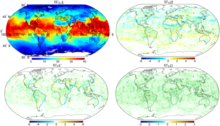
As explained, the wavelet decomposition provides a suitable transformation that gives rise to a sparse representation for a state vector with local transitions and singularities. Here, we use the redundant discrete Stationary Wavelet Transform (SWT) [28]. Owing to its redundancy and translation invariance, the SWT provides a richer representation [3] for sparse expression of complex processes than the classic orthogonal wavelet decomposition [25]. Figure 1 demonstrates the wavelet coefficients of a global three-day average product (09/01 to 09/03/2002) of the level-II water vapor mass mixing ratio (MMR) near the earth’s surface. The three-day integration of data granules allows to obtain an almost seamless estimate of the global MMR field with minimal averaging on the overlapping grids.

As is evident in Figure 1, the high-pass wavelet coefficients are markedly sparse as most of the coefficients are near zero. It is seen that the horizontal wavelet coefficients capture the latitudinal moisture variability while the vertical coefficients mostly encapsulate the sharp zonal moisture transitions across land-ocean interfaces. The large wavelet coefficients over ocean are mostly influenced by the presence of sharp moisture gradients due to convective updrafts in the Intertropical Convergence Zone (ITCZ) and downdrafts near the subtropical ridges. Over land, large coefficients of surface moisture are mainly concentrated near ocean-land interfaces and major mountainous features covered with snow such as the Himalayas and Andes. In addition, owing to the migration of the ITCZ over land, we see large horizontal coefficients, for instance over the semi-arid Sahel, where the climate and vegetation regime exhibits a sharp transition. Isolated moisture highs can also be traced in the coefficients over the boundaries of sufficiently large inland water bodies such as the Caspian Sea.

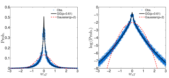
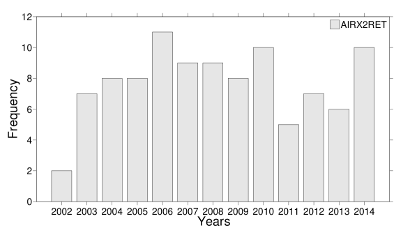
To study the presence of sparsity and characterize it as a priori knowledge, we randomly collected a database containing 100 days of the AIRS/AMSU level II standard retrieval products, from 2002 to 2014 (see Figure A.1 in the appendix). Figure 2 demonstrates the overlaid probability masses (circles) for the high-pass wavelet coefficients of the near surface water vapor MMR for all of the samples. We see that the sparsity of the wavelet coefficients manifests itself as a large probability mass around zero with extended tails much thicker than the Gaussian density. In this figure the solid line is the fitted Generalized Gaussian (GG) distribution with the following form:

$$\mathcal{P}_{X}\left(x\right)=\frac{p}{2\sigma\Gamma\left(1/p\right)}\exp\left(-\left|\frac{x}{\sigma}\right|^{p}\right),$$ (1)

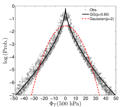
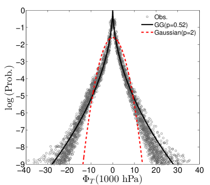
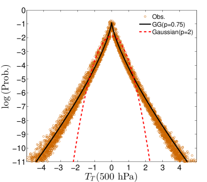
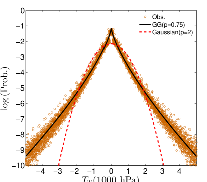
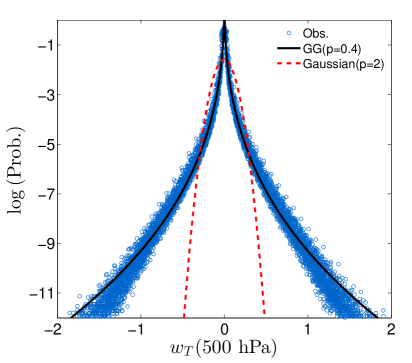
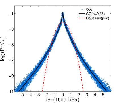
where the Gamma function is $\Gamma\left(z\right)=\int_{0}^{\infty}e^{-t}\,t^{z-1}\,dt$ for $z>0$ and the non-negative parameters $p$ and $\sigma$ determine the shape and width of the density, respectively [see, 27]. Evidently, this family of distributions is log-concave for $p\geq 1$ and contains the well-known Gaussian ($p=2$) and Laplace ($p=1$) densities as special cases. Here, we consider the shape parameter $p$ as a measure that characterizes the degree of sparseness, noting that the density tends to the Dirac delta function with maximum nominal sparsity for $p\rightarrow 0$. It is observed that not only the moisture fields but also the temperature and pressure fields are sparse in the wavelet domain and can be well explained by the GG density with a much ticker tail than the Gaussian distribution (Figure A.2-to-A.4 in the appendix). To concisely estimate the shape parameter and thus the sparsity of the wavelet coefficients, we note that the following ratio of the first and second order moments

$$\mathcal{M}\left(p\right)=\frac{\mathbf{m}_{\mathbf{2}}}{\mathbf{m}_{\mathbf{1}}^{\,\,\,2}}=\frac{\Gamma\left(3/p\right)\Gamma\left(1/p\right)}{\left|\Gamma\left(2/p\right)\right|^{2}},$$ (2)

is only a function of the shape parameter in the GG density, where

$$\mathbf{m}_{n}=\int_{-\infty}^{\infty}\left|x\right|^{n}\mathcal{P}_{X}(x)\,dx.$$ (3)

Figure 3: Demonstration of sparsity of the wavelet coefficients of the global fields of geopotential heights [meters], temperature [Kelvin] and water vapor mass mixing ratio [g/Kg dry air] through a statistical moment diagram. The moments are computed from 100 randomly sampled days of AIRS level II standard retrievals, from the earth surface up to 200 hPa. Top-to-bottom panels from left-to-right are: the first (x-axis) and second (y-axis) order moment-pairs of the wavelet coefficients for the fields of geopotential heights (GP_Height); surface (TSurfStd) and profiles (TAirStd) of the atmospheric temperatures; and surface (H20MMRSurf) and profiles (H2OMMRStd) of the water vapor mass mixing ratios. The lines with slope $\mathcal{M}\left(p\right)$ (see equation 2) partition the moment space into sparser ($p\leq 1$) and denser ($p>1$) representations in the wavelet domain. All of the studied fields exhibit remarkable sparsity in the wavelet domain as in all cases $p\leq 1$.

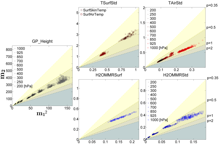
Figure 3 demonstrates the first versus the second-order moments of the high-pass wavelet coefficients of the geopotential heights [meters], temperature [Kelvin] and moisture MMR [g/kg dry air] fields, for all of the retrievals over the 100 sampled days. In this figure, the shaded areas stratify the probability continuum of the GG density for sparser ($p\leq 1$) and denser ($p>1$) representation of the wavelet coefficients in terms of the moment ratio in equation (2). We can see that for all states of interest, the sparsity is measured by $p\leq 1$ throughout the studied atmospheric depth (see, Table A.1 in the appendix). For the geopotential heights, the magnitude of the moment pairs and their spread grow almost linearly from high to low pressure levels, while higher pressure fields are slightly sparser than the low-pressure ones (Figure 3, middle-row panel). The sparseness of the temperature fields is relatively pressure-independent (Figure 3, top-row panels). As the air temperature contains more frequent sharp transitions near the earth surface, we consistently see larger moments of the wavelet coefficients at higher-pressure levels. As is evident, surface skin and air temperature fields are among the sparsest fields with $p\cong 0.5$. It is seen that the surface skin temperatures exhibit stronger sparsity with slightly smaller shape parameter $p$, compared to the near surface air temperatures. This observation reflects the fact that the fields of surface skin temperatures contain sharper transitions and thus larger wavelet coefficients, compared to the surface air temperatures, partly because of the mixing and diffusive effects of the planetary boundary layer. The moisture fields are also sparse but their sparsity exhibits a notable pressure-dependence (Figure 3, bottom-row panels). Specifically, it can be seen that moisture fields at higher-pressure levels are less sparse with larger $p$ values than in the upper atmosphere. In other words, compared to the moist lower atmosphere, it seems that the spatial distribution of moisture in the dry upper atmosphere is relatively invariant in space, giving rise to a large number of near zero fluctuations captured by the wavelet coefficients. However, the upper atmosphere moisture fields perhaps contain localized and sharp transitions, partly due to intermittent deep convections and movements of the jet streams, giving rise to a heavier tail and sparser distribution of the wavelet coefficients.

3 Compressive Sensing of Land Atmospheric States

Owing to the sub-hourly and sub-kilometer evolution of the mesoscale land surface-atmospheric dynamics, spaceborne remote sensing at the Nyquist-Shannon rate seems costly and often infeasible for now, at least from a hardware perspective. In this section, we provide a brief introduction to Compressive Sensing (CS) and then present experimental evidence that owing to the observed sparsity, the global fields of temperate and humidity can be recovered with sufficient accuracy using only a few incoherent/random samples.

As previously mentioned, CS is an emerging field in statistical estimation theory that allows to reconstruct sparse state vectors only from a few randomized measurements. Specifically, for a perfect reconstruction of a continuous state of interest from its discrete samples, the classic Nyquist-Shannon sampling theorem demands a uniform sampling rate of at least twice the highest frequency content of the state variable of interest. However, central results of CS suggest that we can recover a sparse state from a much smaller set of measurements than those required by the Nyquist-Shannon criterion. In particular, let us assume that the state $\mathbf{x}\in\mathfrak{R}^{m}$ is represented by an $m$-element vector which has $k$ non-zero elements, either in the ambient or a suitable transform domain (e.g., wavelet). Furthermore, let us consider that a set of under-sampled measurements $\mathbf{y}\in\mathfrak{R}^{n}$, that is $n\ll m$, are related to the true state $\mathbf{x}$, through the following linear model

$$\mathbf{y=}\mathbf{Hx}+\mathbf{v},$$ (4)

where $\mathbf{v}\in\mathfrak{R}^{n}$ represents an error with an $n$-by-$n$ covariance matrix $\mathbf{R}\in\mathfrak{R}^{n\times n}$, and $\mathbf{H}\in\mathfrak{R}^{n\times m}$ denotes a specifically designed “sensing matrix” that linearly samples the state variable of interest. Notice that rather than sampling the state uniformly at specific points in time and space, CS "samples" it as inner products between the state of interest and rows of the linear sensing matrix $\mathbf{H}$. The CS theory proves [see, 5] that we can recover, with high-degree of accuracy, the state of interest from a few randomly chosen linear measurements $\mathbf{y}$ via the $\ell_{1}$-norm regularization of a classic least-squares estimator as follows:

$$\underset{\mathbf{x}}{\text{minimize}}\;\left\{\left\|\mathbf{y}-\mathbf{H}\mathbf{x}\right\|_{\mathbf{R}}^{2}+\lambda\left\|\mathbf{W}\mathbf{x}\right\|_{1}\right\},$$ (5)

where, the $\ell_{1}$-norm is defined by $\left\|\mathbf{x}\right\|_{1}=\Sigma_{i=1}^{m}\left|x_{i}\right|$, the quadratic norm is $\left\|\mathbf{x}\right\|_{\mathbf{R}}=\mathbf{x}^{T}\mathbf{R}^{-1}\mathbf{x}$, $\mathbf{W}$ represents a suitable sparsifying transformation (e.g., wavelet) and $\lambda>0$ is a regularization parameter. Minimization of the $\ell_{1}$-norm promotes sparsity while the quadratic penalty ensures fidelity of the solution to the observations. Note that from the Bayesian statistical point of view, the $\ell_{1}$-norm regularization is equivalent to assuming that the underlying sparsity can be a priori explained by the GG density with $p=1$.

The design of the sensing matrix $\mathbf{H}$ plays a critical role in the success of a CS reconstruction. Practically, this matrix has to sample the underlying state $\mathbf{x}$ incoherently to assure a quasi-uniform spreading of the “uncaptured energy” across the entire field, for avoiding aliasing and blurring artifacts in the reconstruction process [24]. Theoretically, the CS recovery in problem (5) succeeds with high probability when the matrix $\mathbf{H}\mathbf{W}^{T}$ (which is the multiplication of $\mathbf{H}$ with the transpose of $\mathbf{W}$) behaves like an orthogonal transformation when operating on a sparse state. Such a behavior has been precisely characterized by a few mathematical notions, including the Restricted Isometric Property (RIP) by Candes and Tao [5], and the Spark and Mutual-Coherence by Donoho and Elad [10]. In our analysis, the sensing matrix $\mathbf{H}$ is obtained by random sampling of a few rows of the identity matrix, which is equivalent to obtaining the observations from a small number of pixels in the satellite field of view. While, CS problem (5) often succeeds with this incoherent sensing matrix, $\mathbf{H}\mathbf{W}^{T}$ cannot be guaranteed to have the RIP and the theoretical study of similar sampling schemes is a topic of an ongoing research [31, 22]

Figure 4: CS reconstruction of the surface skin temperature [Kelvin] (left column, 01/01/2002) and surface water vapor mass mixing ratio [g/kg dry air] (right column, 09/09/2002) for all daily ascending orbital tracks. The originally retrieved fields (top row), the randomly under-sampled fields (middle row), and the CS reconstructed fields (bottom row). The under-sampled fields only contain 45% of randomly chosen pixels, which are also corrupted with a white Gaussian noise.

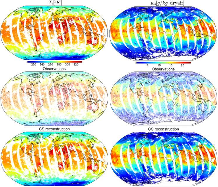
The top panels in Figure 4 demonstrate ascending granules of the AIRS/AMSU level II standard retrievals of the surface skin temperature on 01/01/2002 and near surface water vapor MMR on 09/09/2002, respectively. In these figures, the data granules are projected onto a regular grid with 0.5-degree resolution using the nearest-neighbor interpolation. To implement the CS reconstructions, all the pixels of the original fields were first scaled into the range between 0 and 1. Then, we randomly sampled only 45% of the retrieved pixels and added a small zero-mean white Gaussian noise with standard deviation $10^{-3}$ to those samples (Figure 4 middle panels). The results of the CS reconstruction are demonstrated in the bottom panels of Figure 4. In our experiments, we used the Fast Iterative Shrinkage-Thresholding Algorithm by Beck and Teboulle [2]. The regularization parameter in problem (5) needs to be determined empirically. We chose $\lambda=0.02$, which we found to work well for our case studies (see, Kim et al. [21] for feasible ranges of $\lambda$). Note that, owing to the chosen sensing matrix, the initial energy (sum of squares) of the error in these experiments is approximately 55% of the total energy of the original fields. After CS reconstruction the energy of error is less than 0.03% and 2% of the total energy in the examined temperature and moisture fields, respectively. Although CS recovers remarkably well the large-scale features of the moisture-temperature fields, a close inspection shows that some isolated moisture highs have not been well captured in the reconstruction process (e.g., over the Red Sea), especially near the swath edges. We empirically observed that under the same sampling scheme, typically, the surface temperature fields can be recovered with less reconstruction error than that of the moisture fields, which may be partly due to the stronger sparsity prior (smaller $p$ values) in the temperature fields (Table A.1 in the appendix). We also found that for a randomized sample size of more than 50-to-60% of the total pixels, the reconstruction is almost perfect and CS recovers well even the small-scale features of the moisture fields. Typically, the reconstruction quality severely degrades, and it may diverge, for sample sizes of less than 20% of the total pixels.

4 Concluding Remarks

We have provided compelling evidence that the spatial structure of the fields of temperature-moisture and geopotential heights is sparse in the wavelet domain. This result is key for supporting further developments of the recently suggested sparsity-promoting data assimilation methods. Furthermore, exploiting the sparsity prior, we provided promising results on the use of Compressive Sensing (CS) theory for efficient reconstruction of these primary state variables from a few linear random measurements/retrievals. While progress has been made recently in developing sparse digital image acquisition in visible bands [12], development of sparse-remote-sensing instruments for earth observations from space, in microwave and infrared wavelengths, remains an important challenge in the coming years. However, our results suggest that, even under the current sensing protocols, only a few randomly chosen pixel-samples of the primary land-atmospheric states can be advantageously exploited for a speedy reconstruction of the entire sensor’s field of view with a notable degree of accuracy. Similar to the prominent applications of CS in rapid Magnetic Resonance Imaging [24], further research is needed to explore practical randomized scanning strategies, compatible with the currently used scanning geometries (e.g., conical, across track), to advance applications of CS for more efficient and faster retrievals of geophysical states from space. Clearly, the implications of such a capability cannot be overstated for real-time tracking and data assimilation of extreme land-atmospheric phenomena in global early warning systems.

5 Acknowledgment

The authors acknowledge support provided by two NASA Global Precipitation Measurement grants (NNX13AG33G and NNX13AH35G) and an NSF grant (DMS-09-56072). The support by the K. Harrison Brown Family Chair and the Joseph T. and Rose S. Ling chair is also gratefully acknowledged. The AIRS/AMSU-A (version 6) data were obtained from the NASA’s Goddard Earth Sciences Data and Information Services Center (GES DISC), which are freely accessible at http://disc.sci.gsfc.nasa.gov/AIRS/data-holdings. The authors also would like to thank Dr. Jarvis Haupt at the University of Minnesota for his offered insights and helpful discussions.

6 Appendix

This appendix contains some figures and descriptions, which are important for clarity and further support of the main arguments of the paper. Specifically, using the standard AIRS/AMSU level II retrievals, this document provides additional evidence supporting the idea that the global fields of temperature-humidity and geopotential heights are sparse in the wavelet domain. Furthermore, we provide complementary descriptions regarding to the design and interpretation of the presented Compressive Sensing (CS) reconstruction experiments.

Appendix A Evidence of Sparsity

Here, Table A.1 shows the median and 95% confidence bound of the computed shape parameters of the GG distribution, from the moments shown in Figure 3. Furthermore, supplementary Figure A.1 shows the frequency histogram of the days for which the standard AIRS level II retrievals are used in this study. Figures A.2, A.3, and A.4 provide further evidence that the fields of geopotential height, temperature and moisture are sparse in the wavelet domain and their representation coefficients can be well explained by the Generalized Gaussian (GG) distribution.

Figure A.1: Annual frequency histogram for 100 sampled days of the AIRS level II standard retrievals in calendar years 2002 to 2014. The sampled data are used to infer sparsity of the fields of geopotental height, temperature and moisture at different pressure levels.

Figure A.2: Sparsity in the fields of geopotential height. Left-to-right panels: the overlaid empirical probability masses (circles) of the wavelet coefficients for the geopotential heights [m] at 500 hPa (left panel) and 1000 hPa (right panel). The results are obtained from the 100 sampled daily retrievals of the AIRS level II products (see, Figure A.1). Here, $\Phi_{T}=\left[\Phi_{H},\,\Phi_{V},\,\Phi_{D}\right]$ stacks all of the horizontal, vertical and diagonal high-pass wavelet coefficients at a single decomposition level. The solid (black) and broken (red) lines are the fitted GG and Gaussian distributions, respectively.

Figure A.3: Sparsity in the temperature fields. The overlaid empirical probability masses (circles) of the wavelet coefficients for the air temperature [Kelvin] fields at pressure levels 500 hPa (left panel) and 1000 hPa (right panel). Please see caption of Figure A.2 for relevant explanations.

Figure A.4: Sparsity in the moisture fields. The overlaid empirical probability masses (circles) of the wavelet coefficients for the fields of the water vapor mass mixing ratio [g/kg dry air] at pressure levels 500 hPa (left panel) and 1000 hPa (right panel). Please see caption of Figure A.2 for relevant explanations.

	GP_Height	SurfSkinTemp	SurfAirTemp	TAirStd	H2OMMRSurf	H2OMMRStd
Median	0.63	0.50	0.59	0.76	0.61	0.40
$\text{CI}_{95}$	$0.51-0.70$	$0.48-0.53$	$0.54-0.63$	$0.64-0.84$	$0.56-0.67$	$0.33-0.66$

Table A.1: The median and the 95% confidence interval (${\rm CI}_{95}$) for the computed shape parameters of the Generalized Gaussian density, from the moments of the wavelet coefficients shown in Figure 3. The shape parameters are obtained by solving equation (2) for $p$ using the bisection method.

Appendix B Sparsity Prior and Compressive Sensing

In this section, we provide more details on how sparsity can be characterized as a prior knowledge and explain the statistical interpretation of the CS problem in equation (5). To be more precise, let us assume that a finite dimensional land-atmospheric state vector $\mathbf{x}\in\mathfrak{R}^{m}$ can be represented by its wavelet coefficients $\mathbf{c}\in\mathfrak{R}^{d}$ obtained through a matrix-vector multiplication, that is $\mathbf{c}=\mathbf{W}\mathbf{x}$, where the rows of $\mathbf{W}\in\mathfrak{R}^{d\times m}$ contain the wavelet bases or frames of choice for which $\mathbf{W}^{T}\mathbf{W}=\mathbf{I}$, where $\left(\cdotp\right)^{T}$ denotes transposition. Assuming that the coefficients are independent and can be well explained by the GG density, it implies that the prior distribution of the state vector of interest admits the following multivariate form:

$$\log\,p\left(\mathbf{x}\right)\propto-\lambda\left\|\mathbf{W}\mathbf{x}\right\|_{p}^{p},$$ (S1)

where the $\ell_{p}$-norm is $\left\|\mathbf{x}\right\|_{p}^{p}=\Sigma_{i=i}^{m}\left|x_{i}\right|^{p}$ and $\lambda>0$ collectively encodes the width parameter of the density. Clearly, from the Bayesian perspective, this a priori knowledge can be used to obtain an a posteriori estimate of the land-atmospheric state of interest. Specifically, let us assume that a set of under-sampled observations $\mathbf{y}\in\mathfrak{R}^{n}$ are related to the true state $\mathbf{x}\in\mathfrak{R}^{m}$, that is $n<m$, via the following linear model

$$\mathbf{y=}\mathbf{Hx}+\mathbf{v},$$ (S2)

where $\mathbf{v}\in\mathfrak{R}^{n}$ is a length-n error vector of the Gaussian nature with an $n$-by-$n$ covariance matrix $\mathbf{R}\in\mathfrak{R}^{n\times n}$, and $\mathbf{H}\in\mathfrak{R}^{n\times m}$ denotes the sensing matrix. The linear system of equations in (S2) is under-determined for which the maximum likelihood estimator does not yield a unique solution. Clearly, given the observation y, the maximum a posterior (MAP) estimate of the true state can be derived as follows:

$$\mathbf{\hat{\mathbf{x}}}_{\text{MAP}} =\underset{\mathbf{x}}{\text{argmax}}\;p\left(\mathbf{x}|\mathbf{y}\right)$$ (S3)

$$=\underset{\mathbf{x}}{\text{argmin}}\;\left\{-\log\,p\left(\mathbf{y}|\mathbf{x}\right)-\log\,p\left(\mathbf{x}\right)\right\}.$$

Thus, one can easily see that $\hat{\mathbf{x}}_{\text{MAP}}$ can be obtained by solving the following minimization problem

$$\underset{\mathbf{x}}{\text{minimize}}\;\left\{\left\|\mathbf{y}-\mathbf{H}\mathbf{x}\right\|_{\mathbf{R}}^{2}+\lambda\left\|\mathbf{W}\mathbf{x}\right\|_{p}^{p}\right\},$$ (S4)

or alternatively by solving its counterpart in the wavelet domain

$$\underset{\mathbf{c}}{\text{minimize}}\;\left\{\left\|\mathbf{y}-\mathbf{H}\mathbf{W}^{{T}}\mathbf{c}\right\|_{\mathbf{R}}^{2}+\lambda\left\|\mathbf{c}\right\|_{p}^{p}\right\},$$ (S5)

where $\left\|\mathbf{x}\right\|_{\mathbf{R}}^{2}=\mathbf{x}^{{T}}\mathbf{R}^{-1}\mathbf{x}$. By obtaining the MAP estimate of the wavelet coefficients $\hat{\mathbf{c}}_{{\rm MAP}}$ from problem (S5), obviously one can compute the state of interest as $\hat{\mathbf{x}}_{{\rm MAP}}=\mathbf{W}^{T}\mathbf{\,\hat{c}}_{{\rm MAP}}$. A proper choice of the prior term, often called regularization, may allow us to obtain a unique or stable solution for the under-determined system of equations in (S2). Notice that the sparsest solution of problem (S5) can be naturally achieved in case of $p\rightarrow 0$; however, choices of $p<1$ make this problem non-convex. Therefore, $p=1$ is the smallest value of the shape parameter that promotes sparsity while maintaining the problem in the realm of convex optimization. For the CS experiments, we used the Fast Iterative Shrinkage-Thresholding Algorithm in [2] to solve the following problem in the wavelet domain:

$$\underset{\mathbf{c}}{\text{minimize}}\;\left\{\left\|\mathbf{y}-\mathbf{H}\mathbf{W}^{{T}}\mathbf{c}\right\|_{\mathbf{R}}^{2}+\lambda\left\|\mathbf{c}\right\|_{1}\right\},$$ (S6)

and then recovered the state of interest in ambient domain from the estimated coefficients. As explained in the main body of the paper, for further theoretical explanation of random sampling and it implication for the $\ell_{1}$-norm reconstruction, the reader may refer to the original work by Candes and Tao [5], while more practical applications in the magnetic resonance imaging can be found in [24].

References

- [1]
- Beck and Teboulle [2009] Beck, A., and M. Teboulle (2009), A Fast Iterative Shrinkage-Thresholding Algorithm for Linear Inverse Problems, SIAM J. Imaging Sci., 2(1), 183–202, doi:10.1137/080716542.
- Bodmann et al. [2011] Bodmann, B. G., P. G. Casazza, and G. Kutyniok (2011), A quantitative notion of redundancy for finite frames, Appl. Comput. Harmonic Anal., 30(3), 348 – 362, doi:10.1016/j.acha.2010.09.004.
- Candes and Romberg [2006] Candes, E. J., and J. Romberg (2006), Quantitative robust uncertainty principles and optimally sparse decompositions, Found. Comput. Math., 6(2), 227–254, doi:10.1007/s10208-004-0162-x.
- Candes and Tao [2005] Candes, E. J., and T. Tao (2005), Decoding by linear programming, IEEE Trans. Inform. Theory., 51(12), 4203–4215, doi:10.1109/TIT.2005.858979.
- Candes and Tao [2006] Candes, E. J., and T. Tao (2006), Near-optimal signal recovery from random projections: Universal encoding strategies?, IEEE Trans. Inform. Theory., 52(12), 5406–5425, doi:10.1109/TIT.2006.885507.
- Candes et al. [2006a] Candes, E. J., J. Romberg, and T. Tao (2006a), Robust uncertainty principles: exact signal reconstruction from highly incomplete frequency information, IEEE Trans. Inform. Theory., 52(2), 489–509, doi:10.1109/TIT.2005.862083.
- Candes et al. [2006b] Candes, E. J., J. K. Romberg, and T. Tao (2006b), Stable signal recovery from incomplete and inaccurate measurements, Commun. Pure Appl. Math., 59(8), 1207–1223, doi:10.1002/cpa.20124.
- Donoho [2006] Donoho, D. (2006), Compressed sensing, IEEE Trans. Inform. Theory., 52(4), 1289–1306, doi:10.1109/TIT.2006.871582.
- Donoho and Elad [2003] Donoho, D. L., and M. Elad (2003), Optimally sparse representation in general (nonorthogonal) dictionaries via minimization, Proceedings of the National Academy of Sciences, 100(5), 2197–2202, doi:10.1073/pnas.0437847100.
- Du et al. [2012] Du, J., F. Cooper, and S. Fueglistaler (2012), Statistical analysis of global variations of atmospheric relative humidity as observed by airs, J. Geophys. Res., 117(D12), doi:10.1029/2012JD017550.
- Duarte et al. [2008] Duarte, M., M. Davenport, D. Takhar, J. Laska, T. Sun, K. Kelly, and R. Baraniuk (2008), Single-pixel imaging via compressive sampling, IEEE Signal. Proc. Mag., 25(2), 83–91, doi:10.1109/MSP.2007.914730.
- Ebtehaj et al. [2014] Ebtehaj, A., M. Zupanski, G. Lerman, and E. Foufoula-Georgiou (2014), Variational Data Assimilation via Sparse Regularisation, Tellus A., 66, 2178, doi:http://dx.doi.org/10.3402/tellusa.v66.21789.
- Ebtehaj and Foufoula-Georgiou [2013] Ebtehaj, A. M., and E. Foufoula-Georgiou (2013), On Variational Downscaling, Fusion and Assimilation of Hydro-meteorological States: A Unified Framework via Regularization, Water Resour. Res, 49(9), 5944–5963, doi:10.1002/wrcr.20424.
- Eldar and Kutyniok [2012] Eldar, Y., and G. Kutyniok (2012), Compressed Sensing: Theory and Applications, Compressed Sensing: Theory and Applications, Cambridge University Press, NY.
- Entekhabi et al. [2010] Entekhabi, D., E. Njoku, P. O’Neill, K. Kellogg, W. Crow, W. Edelstein, J. Entin, S. Goodman, T. Jackson, J. Johnson, J. Kimball, J. Piepmeier, R. Koster, N. Martin, K. McDonald, M. Moghaddam, S. Moran, R. Reichle, J.-C. Shi, M. Spencer, S. Thurman, L. Tsang, and J. Van Zyl (2010), The soil moisture active passive (SMAP) mission, Proceedings of the IEEE, 98(5), 704–716, doi:10.1109/JPROC.2010.2043918.
- Ferguson and Wood [2010] Ferguson, C. R., and E. F. Wood (2010), An evaluation of satellite remote sensing data products for land surface hydrology: Atmospheric infrared sounder, J. Hydrometeor., 11(6), 1234–1262, doi:10.1175/2010JHM1217.1.
- Foufoula-Georgiou et al. [2014] Foufoula-Georgiou, E., A. Ebtehaj, S. Zhang, and A. Hou (2014), Downscaling Satellite Precipitation with Emphasis on Extremes: A Variational -Nrom Regularization in the Derivative Domain, Surv. Geophys., pp. 1–19, doi:10.1007/s10712-013-9264-9.
- Freitag et al. [2012] Freitag, M. A., N. K. Nichols, and C. J. Budd (2012), Resolution of sharp fronts in the presence of model error in variational data assimilation, Quart. J. Roy. Meteor. Soc., 139, 749–757, doi:10.1002/qj.2002.
- Hou et al. [2013] Hou, A. Y., R. K. Kakar, S. Neeck, A. A. Azarbarzin, C. D. Kummerow, M. Kojima, R. Oki, K. Nakamura, and T. Iguchi (2013), The global precipitation measurement mission, Bull. Amer. Meteor. Soc., 95(5), 701–722, doi:10.1175/BAMS-D-13-00164.1.
- Kim et al. [2007] Kim, S.-J., K. Koh, M. Lustig, S. Boyd, and D. Gorinevsky (2007), An Interior-Point Method for Large-Scale l1-Regularized Least Squares, IEEE J. Sel. Topics Signal Process., 1(4), 606–617, doi:10.1109/JSTSP.2007.910971.
- Krahmer and Ward [2014] Krahmer F., and R. Ward. Stable and robust sampling strategies for compressive imaging. IEEE Trans. Image Process., 23(2):612–622, Feb 2014.
- Le Marshall et al. [2006] Le Marshall, J., J. Jung, J. Derber, M. Chahine, R. Treadon, S. J. Lord, M. Goldberg, W. Wolf, H. C. Liu, J. Joiner, J. Woollen, R. Todling, P. van Delst, and Y. Tahara (2006), Improving Global Analysis and Forecasting with AIRS, Bull. Amer. Meteor. Soc., 87(7), 891–894, doi:10.1175/BAMS-87-7-891.
- Lustig et al. [2008] Lustig, M., D. L. Donoho, J. M. Santos, J. M. Pauly (2008), Compressed Sensing MRI, IEEE Signal Process. Mag., 25, 72–82, doi:10.1109/MSP.2007.914728.
- Mallat [1989] Mallat, S. (1989), A theory for multiresolution signal decomposition: the wavelet representation, IEEE Trans. Pattern Anal. Mach. Intell., 11(7), 674–693, doi:10.1109/34.192463.
- Mallat [2009] Mallat, S. (2009), A wavelet tour of signal processing: the sparse way, 3rd ed., 805 pp., Elsevier /Academic Press, Burlington, MA.
- Nadarajah [2005] Nadarajah, S. (2005), A generalized normal distribution, J. Appl. Stat., 32(7), 685–694.
- Nason and Silverman [1995] Nason, G. P., and B. W. Silverman (1995), The Stationary Wavelet Transform and some Statistical Applications, Lecture Notes in Statist., 103, 281–299.
- Olsen et al. [2013] Olsen, T. E., E. Fetzer, G. Hulley, E. Manning, J. Blaisdell, L. Iredell, J. Susskind, J. Warner, Z. Wei, W. Blackwell, E. Maddy (2013), AIRS/AMSU/HSB Version 6 Level 2 Product User Guide, pp. 134, available at http://disc.sci.gsfc.nasa.gov/AIRS/documentation/v6_docs.
- Pagano et al. [2003] Pagano, T., H. Aumann, D. Hagan, and K. Overoye (2003), Prelaunch and in-flight radiometric calibration of the Atmospheric Infrared Sounder (AIRS), IEEE Trans. Geosci. Remote., 41(2), 265–273, doi:10.1109/TGRS.2002.808324.
- Rauhut and Ward [2012] Rauhut H., and R. Ward. Sparse legendre expansions via l1-minimization. Journal of Approximation Theory, 164(5):517–533, 2012.
- Reale et al. [2008] Reale, O., J. Susskind, R. Rosenberg, E. Brin, E. Liu, L. P. Riishojgaard, J. Terry, and J. C. Jusem (2008), Improving forecast skill by assimilation of quality-controlled AIRS temperature retrievals under partially cloudy conditions, Geophys. Res. Lett., 35(8), L08,809.
- Reale et al. [2009] Reale, O., W. K. Lau, J. Susskind, E. Brin, E. Liu, L. P. Riishojgaard, M. Fuentes, and R. Rosenberg (2009), AIRS impact on the analysis and forecast track of tropical cyclone Nargis in a global data assimilation and forecasting system, Geophys. Res. Lett., 36(6), doi:10.1029/2008GL037122.
- Reale et al. [2012] Reale, O., K. Lau, J. Susskind, and R. Rosenberg (2012), AIRS impact on analysis and forecast of an extreme rainfall event (Indus River Valley, Pakistan, 2010) with a global data assimilation and forecast system, J. Geophys. Res., 117, D08,103, doi:doi:10.1029/2011JD017093.
- Susskind et al. [2003] Susskind, J., C. Barnet, and J. Blaisdell (2003), Retrieval of atmospheric and surface parameters from AIRS/AMSU/HSB data in the presence of clouds, IEEE Trans. Geosci. Remote., 41(2), 390–409, doi:10.1109/TGRS.2002.808236.
- Susskind et al. [2011] Susskind, J., J. Blaisdell, L. Iredell, and F. Keita (2011), Improved Temperature Sounding and Quality Control Methodology Using AIRS/AMSU Data: The AIRS Science Team Version 5 Retrieval Algorithm, IEEE Trans. Geosci. Remote., 49(3), 883–907, doi:10.1109/TGRS.2010.2070508.
- Tian et al. [2006] Tian, B., D. E. Waliser, E. J. Fetzer, B. H. Lambrigtsen, Y. L. Yung, and B. Wang (2006), Vertical Moist Thermodynamic Structure and Spatial–Temporal Evolution of the MJO in AIRS Observations, J. Atmos. Sci., 63(10), 2462–2485, doi:10.1175/JAS3782.1.
- Wu et al. [2012] Wu, L., H. Su, R. G. Fovell, B. Wang, J. T. Shen, B. H. Kahn, S. M. Hristova-Veleva, B. H. Lambrigtsen, E. J. Fetzer, and J. H. Jiang (2012), Relationship of environmental relative humidity with north atlantic tropical cyclone intensity and intensification rate, Geophys. Res. Lett., 39(20), doi:10.1029/2012GL053546.