Pseudospin S=1 formalism and skyrmion-like excitations in the three body constrained extended Bose-Hubbard model
Abstract
We have focused in the paper on the most prominent and intensively studied S=1 pseudospin formalism for extended bosonic Hubbard model (EHBM) with truncation of the on-site Hilbert space to the three lowest occupation states n = 0, 1, 2. The EHBM Hamiltonian is a paradigmatic model for the highly topical field of ultracold gases in optical lattices. Generalized non-Heisenberg effective pseudospin Hamiltonian does provide a deep link with boson system and physically clear description of ”the myriad of phases” from uniform Mott insulating phases and density waves to two types of superfluids and supersolids. We argue that the 2D pseudospin system is prone to a topological phase separation and focus on several types of unconventional skyrmion-like topological structures in 2D boson systems, which have not been analysed till now. The structures are characterized by a complicated interplay of insulating and the two superfluid phases with a single boson and two-boson condensation, respectively.
I Introduction
Since 1989 , the bosonic Hubbard model (see Refs.Fisher, and references therein) has attracted continued interest due to its very rich ground state phase diagram and large opportunities of a direct experimental realization in systems of ultracold bosonic atoms loaded in optical lattices. Such systems offer unique opportunities for studying strongly correlated quantum matter in a highly controllable environment.
The Hamiltonian of the extended bosonic Hubbard model (EBHM) is usually defined as follows
| (1) |
where , , are, respectively, the boson creation, annihilation, and number operators at the lattice site . The boson transfer amplitudes are given by ; and parametrize the Coulomb repulsions between bosons resting at the same and different sites. While causes the bosons to delocalize, promoting a superfluid (SF) phase at weak interactions, and tend to stabilize the conventional Mott insulator (MI) and the density wave (DW) phases when the interaction dominates over the hopping energy scale set by .
Attractive on-site boson-boson interactions allow for the formation of dimers, or bound states of two bosons. The phase diagram then contains the conventional one-boson superfluid (1-BS) with nonvanishing order parameters and and dimer superfluid (2-BS) phase. The 2-BS phase is characterized by the vanishing of the one-boson order parameter () but nonzero pairing correlation (). Apart from the above local order parameters, one can use superfluid stiffness to identify the superfluid states. It is worth noting, the thermal transitions between the 2-BS dimer superfluid and the 1-BS normal fluid are considered in Ref.Kwai, .
When the inter-site boson-boson repulsion is turned on, in addition to the uniform Mott insulating state and two superfluid phases, a dimer checkerboard solid state appears at unit filling, where boson pairs form a solid with checkerboard structure.
Our starting point for theoretical analysis of the 2D extended Bose Hubbard model will assume truncation of the on-site Hilbert space to the three lowest occupation states n = 0, 1, 2 with further mapping of the EBHM Hamiltonian to an anisotropic spin-1 model (see, e.g., Refs.Berg, ). The simplest effective spin-1 model Hamiltonian is
| (2) |
In this space the DW phase corresponds to an antiferromagnetic ordering of the pseudospins in the direction. The MI ground state, on the other hand, includes a large amplitude of the state with on every site with small admixture of states containing tightly bound particle-hole fluctuations ( on nearby sites). The phase can be termed as a quantum paramagnet. The 1-BS and 2-BS superfluid phases correspond to dipole and quadrupole (nematic) pseudospin XY-order, respectively. Generally speaking, one may anticipate the emergence of so-called supersolid phases, or mixed 1-BS+DW (2-BS+DW) phases.
In this paper, we do consider the most general form of the effective S=1 pseudospin Hamiltonian related with the extended Bose-Hubbard model and present a short overview of different phase states. We focus on several types of unconventional skyrmion-like topological structures in 2D boson systems, which have not been analysed till now. The structures are characterized by a complicated interplay of insulating and two superfluid phases. The rest of the paper is organized as follows. Sec.II is devoted to introduction into the pseudospin formalism, in Sec.III we introduce and analyse the effective pseudospin Hamiltonian. In Sec.IV we turn to a short overview of a typical simplified S=1 spin model. Unconventional pseudospin topological structures are considered in Sec.V with a short conclusion in Sec.VI.
II Pseudospin formalism
One strategy to handle with the physics of the extended Bose-Hubbard model with the truncated on-site Hilbert space is to make use of a S=1 pseudospin formalism MM ; Batista+Ortiz and to create model pseudospin Hamiltonian that can reasonably well reproduce both the ground state and important low-energy excitations of the full problem. Standard pseudospin formalism represents a variant of the equivalent operators technique widely known in different physical problems from classical and quantum lattice gases, binary alloys, (anti)ferroelectrics,.. to neural networks. The formalism starts with a finite basis set for a lattice site (triplet in our model). Such an approach differs from well-known pseudospin-particle transformations akin Jordan-Wigner JW or Holstein-Primakoff HP transformation which establish a strict linkage between pseudospin operators and the creation/annihilation operators of the Fermi or Bose type. The pseudospin formalism generally proceeds with a truncated basis and does not imply a strict relation to boson operators that obey the bosonic commutation rules.
The three on-site Fock states can be addressed to form a local Hilbert space of the semi-hard core bosons which can be mapped onto a system of S = 1 centers via a generalization of the Matsubara-Matsuda transformation Batista+Ortiz that also maps the boson density into the local magnetization: . In contrast to the hard-core bosons associated with S = 1/2 magnets, it is possible to study ”Hubbard-like” bosonic gases with on-site density-density (contact) interactions because . Hereafter, we associate the three on-site Fock states with the occupation numbers with the three components of the pseudo-spin (isospin) triplet with , respectively. It is worth noting that very similar S=1 pseudospin formalism was suggested recently Moskvin-11 ; JPCM to describe the triplet of Cu1+, Cu2+, Cu3+ valence states in copper high-temperature superconductors.
The spin algebra includes the three independent irreducible tensors of rank with one, three, and five components, respectively, obeying the Wigner-Eckart theorem Varshalovich
| (3) |
Here we make use of standard symbols for the Wigner coefficients and reduced matrix elements. In a more conventional Cartesian scheme a complete set of the non-trivial pseudo-spin operators would include both and a number of symmetrized bilinear forms , or spin-quadrupole operators, which are linearly coupled to and , respectively
| (4) |
Instead of the three states one may use the Cartesian basis set , or :
| (5) |
so that an on-site wave function can be written in the matrix form as follows Nadya :
| (6) |
with . Obviously, the minimal number of dynamic variables describing an isolated on-site (pseudo)spin center equals to four, however, for a more general situation, when the (pseudo)spin system represents only the part of the bigger system, and we are forced to consider the coupling with the additional degrees of freedom, one should consider all the five non-trivial parameters.
The pseudospin matrix has a very simple form within the basis set:
| (7) |
We start by introducing the following set of S=1 coherent states characterized by vectors and satisfying the normalization constraint Nadya
| (8) |
where and are real vectors that are arbitrarily oriented with respect to some fixed coordinate system in the pseudospin space with orthonormal basis .
The two vectors are coupled, so that the minimal number of dynamic variables describing the (pseudo)spin system appears to be equal to four. Hereafter we would like to emphasize the nature of the vector field: and describe the physically identical states.
It should be noted that in real space the state corresponds to a quantum on-site superposition
| (9) |
Existence of such unconventional on-site superpositions is a principal point of the model. Below instead of and we will make use of a pair of unit vectors and , defined as follows Knig :
For the averages of the principal pseudospin operators we obtain
| (10) |
or
| (11) |
One should note a principal difference between the and quantum systems. The only on-site order parameter in the former case is an average spin moment , whereas in the latter one has five additional ”spin-quadrupole”, or spin-nematic order parameters described by traceless symmetric tensors
| (12) |
Interestingly, that in a sense, the quantum spin system is closer to a classic one () with all the order parameters defined by a simple on-site vectorial order parameter than the quantum spin system with its eight independent on-site order parameters.
The operators () change the -projection of the pseudospin and transform the state into the one. In other words, these can change the occupation number. It should be emphasized that for the pseudospin algebra there are two operators: and , or and that change the pseudo-spin projection (and occupation number) by , with slightly different properties
| (13) |
but
| (14) |
It is worth noting the similar behavior of the both operators under the hermitian conjugation: ; .
The , or operator changes the pseudo-spin projection by with the local order parameter
| (15) |
Obviously, this on-site off-diagonal order parameter is nonzero only when both and are nonzero, or for the on-site superpositions. It is worth noting that the () operator creates an on-site boson pair, or dimer, with a kinematic constraint = 0, that underlines its ”hard-core” nature.
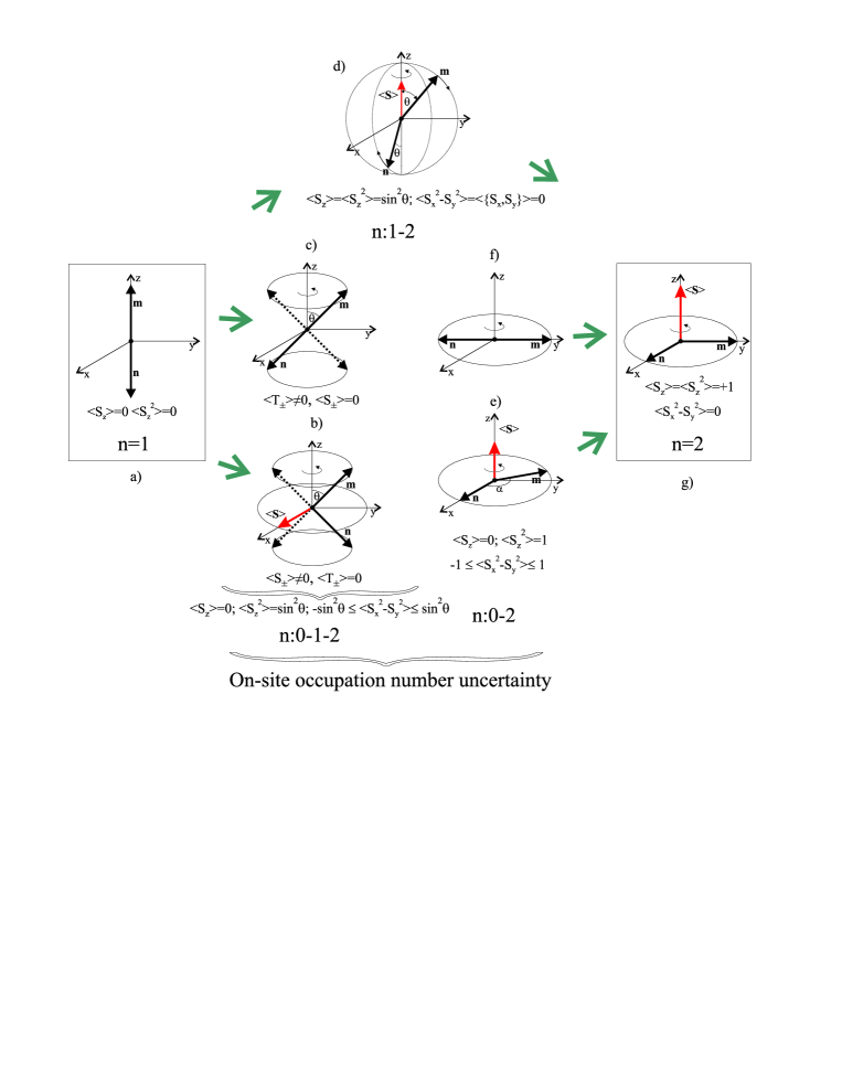
Figure 1 shows orientations of the and vectors which provide extremal values of different on-site pseudospin order parameters given . The center is described by a pair of and vectors directed along Z-axis with = 1. We arrive at the or mixtures if turn or , respectively, into zero. The mixtures are described by a pair of and vectors whose projections on the XY-plane, and , are of the same length and orthogonal to each other: = 0, = with = = for and mixtures, respectively (see Fig. 1).
It is worth noting that for ”conical” configurations in Figs. 1b-1d:
| (16) |
(Fig. 1b);
| (17) |
(Fig. 1c);
| (18) |
(Fig. 1d). Figures 1e,f do show the orientation of and vectors for the local binary mixture , and Fig.1g does for center. It is worth noting that for binary mixtures - and - we arrive at the same algebra of the and operators with , while for ternary mixtures -- these operators describe different excitations. Interestingly that in all the cases the local fraction can be written as follows:
| (19) |
In the bosonic language and are on-site diagonal order parameters, these describe local density and boson nematic order, respectively. The on-site mean values and are the two types of local off-diagonal order parameters that describe one-boson superfluidity, while is a local order parameter of the two-boson, or dimer superfluidity.
III Effective S=1 pseudospin Hamiltonian
General form of the effective pseudospin Hamiltonian which does commute with the z-component of the total pseudospin thus conserving the mean boson density reads as follows Moskvin-11 ; JPCM :
| (20) |
The Hamiltonian can be rewritten to be a sum of potential and kinetic energies, that is of the (”diagonal”) and (”off-diagonal”) terms:
| (21) |
where
| (22) |
and being a sum of one-particle and two-particle transfer contributions
| (23) |
| (24) |
with a boson density constraint:
| (25) |
where is the deviation from a half-filling ().
Hamiltonian corresponds to a classical spin-1 Ising model with a single-ion anisotropy term, or the generalized Blume-Capel model Blume , in the presence of a longitudinal magnetic field. The first single-site term in describes the effects of a bare pseudo-spin splitting and relates with the on-site density-density interactions: =. The second term may be related to a pseudo-magnetic field , which acts as a chemical potential ( is the boson chemical potential, and is a (random) site energy). At variance with the real external field the chemical potential depends both on the parameters of the Hamiltonian (21) and the temperature. The third bilinear and forth biquadratic terms in describe the effects of the short- and long-range inter-site density-density interactions.
plays the role of the kinetic energy where and describe the one- and two-particle inter-site hopping, respectively. Hamiltonian represents an obvious extension of the conventional Hubbard model that assumes that the single particle orbital is infinitely rigid irrespective of occupation number, and has much in common with so-called dynamic Hubbard models Hirsch that describe a correlated hopping. The ST and TT terms describe a density-dependent single-particle hopping. It was Hirsch and coworkers Hirsch who stressed the importance of the density-induced tunneling effects in the condensed-matter context.
However, before mapping the pseudospin model into a discrete free bosonic model, one should take care that the amplitude of the one-particle hoppings in Bose-Hubbard Hamiltonian (1) obey the bosonic commutation relations. This implies that the amplitude of the - process is twice as large as that of - and a factor larger than that of -. It should be noted that within the triplet basis the bosonic annihilation operator reads as follows Berg
| (26) |
In other words, in frames of a standard EBHM approach all the SS, TT, and ST terms in pseudospin kinetic energy are governed by the only Hubbard transfer integral :
| (27) |
while the pseudospin Hamiltonian allows us to describe more complicated transfer mechanisms. The one- and two-particle hopping terms in are of a primary importance for the transport properties of our model system, and deserve special attention. Three (SS-, TT-, and ST-) types of the one-particle hopping terms are governed by the three transfer integrals , , , respectively. Instead of and operators we can introduce two novel operators and as follows
| (28) |
so that the single particle transfer Hamiltonian transforms into
| (29) |
where
| (30) |
All the three terms here have a clear physical interpretation. The first -type term describes one-particle hopping processes - that is a rather conventional motion of the extra boson in the lattice with the on-site occupation or the motion of the boson hole in the lattice with the on-site occupation. The second -type term describes one-particle hopping processes - that is a rather conventional motion of a boson hole in the lattice with the on-site occupation or the motion of a boson in the lattice with the on-site occupation. These hopping processes are typical ones for heavily underfilled () or heavily overfilled () lattices, respectively. It is worth noting that the ST-type contribution of the one-particle transfer differs in sign for the and transfer thus breaking the “particle-hole” symmetry.
The third () term in (29) defines a very different one-particle hopping process - () that is the particle-hole creation/annihilation. It should be noted that the ST-type transfer does not contribute to the reaction.
The two-particle(hole), or dimer hopping is governed by the transfer integral that defines a probability amplitude for the “exchange” reaction -, or the motion of an on-site dimer in the lattice with the on-site occupation or the motion of an on-site hole in the lattice with the on-site occupation.
All the kinetic energies can be rewritten in terms of the Cartesian pseudospin components, if we take into account that
.
| (31) |
Hamiltonian describes two types of a longitudinal long-range diagonal Z-ordering measured by the static structure factors such as
| (32) |
for a pseudospin-dipole order and
| (33) |
for a pseudospin-quadrupole (nematic) order, respectively.
Hamiltonian describes different types of transverse long-range off-diagonal XY-ordering measured by the transverse components of the static structure factors such as
| (34) |
for conventional pseudospin-dipole order or
| (35) |
and
| (36) |
for two types of pseudospin-quadrupole (nematic) order. In conventional bosonic language the structure factors and describe density-density correlations, the and do the single-boson superfluid correlations, while the does the two-boson (on-site dimer) superfluid correlations.
IV Typical simplified S=1 spin model
Despite many simplifications, the effective pseudospin Hamiltonian (21) is rather complex, and represents one of the most general forms of the anisotropic S=1 non-Heisenberg Hamiltonian. Its real spin counterpart corresponds to an anisotropic S=1 magnet with a single-ion (on-site) and two-ion (inter-site bilinear and biquadratic) symmetric anisotropy in an external magnetic field under conservation of the total . Spin Hamiltonian (21) describes an interplay of the Zeeman, single-ion and two-ion anisotropic terms giving rise to a competition of an (anti)ferromagnetic order along Z-axis with an in-plane magnetic order. Simplified versions of anisotropic S=1 Heisenberg Hamiltonian with bilinear exchange have been investigated rather extensively in recent years. Their analysis seems to provide an instructive introduction to description of our generalized pseudospin model.
Typical S = 1 spin Hamiltonian with uniaxial single-site and exchange anisotropies reads as follows:
| (37) |
Correspondence with our pseudospin Hamiltonian points to , , . Usually one considers the antiferromagnet with since, in general, this is the case of more interest. However, the Hamiltonian (37) is invariant under the transformation and a shift of the Brillouin zone for 2D square lattice. The system described by the Hamiltonian (2) can be characterized by local (on-site) spin-linear order parameters and spin-quadratic (quadrupole spin-nematic) order parameters and .
The model has been studied by several methods, e.g., molecular field approximation, spin-wave theories, exact numerical diagonalizations, nonlinear sigma model, quantum Monte Carlo, series expansions, variational methods, coupled cluster approach, self-consistent harmonic approximation, and generalized SU(3) Schwinger boson representation Khajehpour ; Sengupta1 ; Sengupta2 ; Oitmaa ; Pires .
The spectrum of the spin Hamiltonian (37) in the absence of external magnetic field changes drastically as varies from very small to very large positive or negative values. A strong ”easy-plane” anisotropy for large positive favors a singlet phase where spins are in the ground state. This “quadrupole” phase has no magnetic order, and is aptly referred to as a quantum paramagnetic phase (QPM), which is separated from the ”ordered” state by a quantum critical point at some = . This is a quadrupole state with no magnetic order, so that all linear order parameters vanish and only a quadrupole (spin-nematic) order parameter such as is nonzero. The QPM phase consists of a unique ground state with total spin = 0, separated by a gap from the first excited states, which lie in the sectors . It is worth noting that the QPM order differs in principle from the conventional paramagnetic state, because for S = 1 in the classical paramagnetic state = = = 2/3, while in the quantum paramagnetic state = 0, = = 1. Strictly speaking, all the above analysis concerns the typical mean-field approximation (MFA). Beyond the MFA the QPM ground state contains an admixture of states formed by exciton-like tightly bound particle-hole fluctuations ( on nearby sites).
A strong ”easy-axis” anisotropy for large negative , = Pires , favors a spin ordering along , the ”easy axis”, with the on-site (-phase). The order parameter will be ”Ising-like” and long-range (staggered) diagonal order will persist at finite temperature, up to a critical line T. The easy axis antiferromagnetic phase or more complicated long-range spin -order are characterized by the longitudinal component of the static structure factor .
For intermediate values the system is in a gapless XY phase where the spins will be preferentially in the plane (choosing as the hard axis) and the Hamiltonian will have O(2) symmetry. At T = 0 this symmetry will be spontaneously broken and the system will exhibit spin order in some direction, reduced by quantum fluctuations. The broken O(2) symmetry will result in a single gapless Goldstone mode. Although there will be no ordered phase at finite temperature one expects a finite temperature Kosterlitz-Thouless transition. The XY phase has long-range off-diagonal ordering measured by the transverse component of the static structure factor .
For large positive , in the QPM phase, the low energy excitations arise from exciting one of the () sites to () or (). Such a local excitation, actually the effective particle or hole, can then propagate through the lattice due to the transfer terms (quantum fluctuations) in the , forming a well defined quasiparticle (magnon) band with energy . These coherent magnon bands will have an energy gap, which we expect will vanish as . An analytic expression for in the QPM phase has been proposed by Papanicolaou Papanicolaou , based on a generalized Holstein-Primakoff transformation for isotropic -Heisenberg model with the single-site anisotropy. The application of an effective field, , along the z-axis reduces the spin gap linearly in since the field couples to a conserved quantity (total spin along the z-axis). The gap is closed at a critical field (the quantum critical point (QCP)) where the bottom of the = 1 branch of (pseudo)spin excitations touches zero. This QCP belongs to the BEC universality class and the gapless mode of low-energy = 1 excitations remains quadratic for small momenta, because the Zeeman term commutes with the rest of the Hamiltonian.
Both excitation branches in the QPM phase, = (particle/hole) have the same dispersion at zero field, , as expected from time reversal symmetry. A finite splits the branches linearly in : without changing the dispersion. This is a consequence of the fact that the external field couples to the total spin , which is a conserved quantity.
It should be noted that there are three types of two-magnon excitations with = +2, -2, and 0, respectively. Two-magnon bound state with = 0, or coupled particle-hole pair can propagate through the lattice, forming a quasiparticle band.
At least for relatively small negative the lowest energy excitations, in the unperturbed system, consist of a single spin excited from its ordered state to = 0, i.e. . Respective coherent magnon band will have an energy gap at point , which behaves like at small . This reflects, in the easy axis case, the fact that the remnant O(2) symmetry of the Hamiltonian is not spontaneously broken in this case, and so Goldstone modes are absent.
However, for large negative the single-magnon (single-particle) excitations will not be the lowest energy excitations of the system. Their energy will be of order , whereas an excitation with (i.e. ) will have an energy of order as . Such a two-particle (local dimer) excitation, created at a particular site, can again propagate through the lattice, forming a quasiparticle band. We may think of this local dimer as a long-lived virtual two-magnon bound state (bimagnon) where the magnons are bound on the same site.
Hamer et al. Oitmaa have shown that at finite effective field but = 1 the XY phase transforms into a canted antiferromagnetic XY-ZFM phase which appears right above : the spins acquire a uniform longitudinal component and an antiferromagnetically ordered transverse component that spontaneously breaks the U(1) symmetry of global spin rotations along the z-axis. The longitudinal magnetization increases with field and saturates at the fully polarized (FP) state (all = 1) above the saturation field . The FP state corresponds to a bosonic Mott insulator in the language of Bose gases.
The field induced quantum phase transition from the QPM to the XY-ZFM phase is qualitatively different from the transition between the same two phases that is induced by a change of at = 0. If the single-ion anisotropy is continuously decreased at zero applied field, the two excitation branches remain degenerate and the gap vanishes at ( = 0). The low energy dispersion becomes linear at the QPM-CAFM phase boundary for small k. However, the degeneracy between the two branches at = 0 is lifted inside the CAFM phase – one of the branches remains gapless with a linear dispersion at low energy (corresponding to the Goldstone mode of the ordered CAFM state ) whereas the other mode develops a gap to the lowest excitation. the effect of increasing from zero at a fixed is to reduce the gap linearly in with no change of dispersion.
At 0 and 1 the phase diagram of the S = 1 Heisenberg model with uniaxial anisotropy (37) contains an extended spin supersolid (SS) or “biconical” phase XY-ZFIM with a ferrimagnetic -order that does exist over a range of magnetic fields. The model also exhibits other interesting phenomena such as magnetization plateaus and a multicritical point Sengupta1 . The magnetization stays zero up to the critical field, , that marks a quantum phase transition (QPT) to a state with a finite fraction of spins in all the = 0,1 states. This spin supersolid state has a finite as well as finite . The magnetization increases continuously up to = 0.5 at , where there is a second QPT to a second Ising-like state (IS2) where all the = -1 () sites have been flipped to the = 0 () state. At this, remains divergent but drops to zero. Upon further increasing the field, there is a first order transition to a pure XY-AFM phase (CAFM) with the vanishing diagonal order but finite . This situation persists until all the spins have flipped to the = +1 () state (fully polarized, FP phase). The extent of the SS phase decreases with decreasing and vanishes for 1 leaving a second order transition from the SS to the XY (CAFM) phase.
At 0, 0, and 1 the ground state of the spin Hamiltonian (37) corresponds to the easy axis antiferromagnetic phase. At small anisotropy, , the application of an effective field, , along the z-axis induces first a rather conventional spin-flop transition to a pure XY-AFM phase (CAFM) with the vanishing diagonal order but finite ending by the transition to fully polarized ferromagnetic phase. However, at large anisotropy instead of the mean-field first-type (metamagnetic) phase transition - we arrive at an unconventional intermediate phase with spin ferronematic (FNM) order characterized by zero value of the factor but nonzero correlation function Sengupta2 .
The phase diagram in the most interesting intermediate regime can change drastically, if we take into account frustrative effects of next-nearest neighbor couplings or different non-Heisenberg biquadratic interactions Pires . It should be noted that even for simple isotropic 2D- antiferromagnetic Heisenberg model the classical ground state has a Néel order only when , where is the nearest-neighbor and the next-nearest neighbor interaction. However when , the ground state consists of two independent sublattices with antiferromagnetic order. The classical ground state energy does not depend on the relative orientations of both sublattices. However, quantum fluctuations lift this degeneracy and select a collinear order state, where the neighboring spins align ferromagnetically along one axis of the square lattice and antiferromagnetically along the other (stripe-like order).
Turning to spin-boson mapping we note that QPM phase (), fully polarized phases with or correspond to Mott insulating phases, the XY and XY-ZFM orderings correspond to a Bose-Einstein condensate (BEC) of single bosons while FNM phase corresponds a BEC of the boson dimers. The XY-ZFIM phases correspond to supersolids.
The pseudospin Hamiltonian, Eqs.(21)-(24) differs from its simplified version (2) in several points. First, this concerns the density constraint. It is worth noting that the charge density constraint in an uniform pseudospin system can be fulfilled only under some quasidegeneracy. Second, the pseudospin parameters, in particular , , in the effective Hamiltonian (21) can be closely linked to each other. Instead of a simple usually antiferromagnetic XY-exchange term in (2) we should proceed with a significantly more complicated form of the ”transversal” term in the pseudospin Hamiltonian, (21), with inclusion of two biquadratic terms and unconventional ”mixed” asymmetric ST-type term which formally breaks the time inversion symmetry and is absent for conventional spin Hamiltonians. The seemingly main bilinear XY-exchange term in appears to be of the ferromagnetic sign. Along with a simple spin-linear planar XY-mode with nonzero we arrive at two novel spin-quadrupole nematic modes with nonzero and/or . Hereafter we will denote different counterparts of the phases of the simple model (2) as follows: novel XY-phase, ZAFM for Ising-type antiferromagnetic order along -axis, XY-ZFIM for spin supersolid phases with simultaneous XY- and ferrimagnetic orderings along -axis, XY-ZFM for a phase with simultaneous XY- and ferromagnetic orderings along -axis (the analogue of CAFM phase), and ZFM for fully -polarized ferromagnetic phase.
V Topological defects in 2D S=1 pseudospin systems
V.1 Short overview
In the framework of our model the 2D Bose-Hubbard system prove to be in the universality class of the (pseudo)spin 2D systems whose description incorporates static or dynamic topological defects to be natural element both of micro- and macroscopic physics. Depending on the structure of effective pseudo-spin Hamiltonian in 2D-systems the latter could correspond to either in-plane and out-of-plane vortices or skyrmions. Under certain conditions either topological defects could determine the structure of the ground state. In particular, this could be a generic feature of electric multipolar systems with long-range multipolar interactions. Indeed, a Monte-Carlo simulation of a ferromagnetic Heisenberg model with dipolar interaction on a 2D square lattice shows that, as is increased, the spin structure changes from a ferromagnetic one to a novel one with a vortex-like arrangement of spins even for rather small magnitude of dipolar anisotropy Sasaki .
Topological defects are stable non-uniform spin structures with broken translational symmetry and non-zero topological charge (chirality, vorticity, winding number). Vortices are stable states of anisotropic 2D Heisenberg Hamiltonian
| (38) |
with the ”easy-plane” anisotropy when the anisotropy parameter . Classical in-plane vortex () appears to be a stable solution of classical Hamiltonian (38) at ( for square lattice). At stable solution corresponds to the out-of-plane OP-vortex (), at which center the spin vector appears to be oriented along -axis, and at infinity it arranges within -plane. The in-plane vortex is described by the formulas , . The dependence for the out-of-plane vortex cannot be found analytically. Both kinds of vortices have the energy logarithmically dependent on the size of the system.
The cylindrical domains, or bubble like solitons with spins oriented along the -axis both at infinity and in the center (naturally, in opposite directions), exist for the ”easy-axis” anisotropy . Their energy has a finite value. Skyrmions are general static solutions of classical continuous limit of the isotropic () 2D Heisenberg ferromagnet, obtained by Belavin and Polyakov BP from classical nonlinear sigma model. Belavin-Polyakov skyrmion and out-of-plane vortex represent the simplest toy model (pseudo)spin textures BP ; Borisov .
The simplest skyrmion spin texture looks like a bubble domain in ferromagnet and consists of a vortex-like arrangement of the in-plane components of spin with the -component reversed in the centre of the skyrmion and gradually increasing to match the homogeneous background at infinity. The spin distribution within such a classical skyrmion with a topological charge is given as follows BP
| (39) |
where are polar coordinates on plane, the chirality. For , = 0 we arrive at
| (40) |
In terms of the stereographic variables the skyrmion with radius and phase centered at a point is identified with spin distribution , where is a point in the complex plane, . For a multicenter skyrmion we have BP
| (41) |
where , . Skyrmions are characterized by the magnitude and sign of its topological charge, by its size (radius), and by the global orientation of the spin. The scale invariance of skyrmionic solution reflects in that its energy is proportional to topological charge and does not depend on radius and global phase BP . Like domain walls, vortices and skyrmions are stable for topological reasons. Skyrmions cannot decay into other configurations because of this topological stability no matter how close they are in energy to any other configuration.
In a continuous field model, such as, e.g., the nonlinear -model, the ground-state energy of the skyrmion does not depend on its size BP , however, for the skyrmion on a lattice, the energy depends on its size. This must lead to the collapse of the skyrmion, making it unstable. Strong anisotropic interactions, in particular, long range dipole-dipole interactions may, in principle, dynamically stabilize the skyrmions in 2D lattices Abanov .
Wave function of the spin system, which corresponds to a classical skyrmion, is a product of spin coherent states Perelomov . In case of spin
| (42) |
where . Coherent state provides a maximal equivalence to classical state with minimal uncertainty of spin components. The motion of such skyrmions has to be of highly quantum mechanical nature. However, this may involve a semi-classical percolation in the case of heavy non-localized skyrmions or variable range hopping in the case of highly localized skyrmions in a random potential. Effective overlap and transfer integrals for quantum skyrmions are calculated analytically by Istomin and Moskvin Istomin . The skyrmion motion has a cyclotronic character and resembles that of electron in a magnetic field.
The interest in skyrmions in ordered spin systems received much attention soon after the discovery of high-temperature superconductivity in copper oxides skyrmion-cuprates ; skyrmion . Initially, there was some hope that interaction of electrons and holes with spin skyrmions could play some role in superconductivity, but this was never successfully demonstrated. Some indirect evidence of skyrmions in the magnetoresistance of the litium doped lanthanum copper oxide has been recently reported skyrmion-LaLiCuO but direct observation of skyrmions in 2D antiferromagnetic lattices is still lacking. In recent years the skyrmions and exotic skyrmion crystal (SkX) phases have been discussed in connection with a wide range of condensed matter systems including quantum Hall effect, spinor Bose condensates and especially chiral magnets Bogdanov . It is worth noting that the skyrmion-like structures for hard-core 2D boson system were considered by Moskvin et al. bubble in frames of the s=1/2 pseudospin formalism.
V.2 Unconventional skyrmions in (pseudo)spin systems
Different skyrmion-like topological defects for 2D (pseudo)spin S=1 systems as solutions of isotropic spin Hamiltonians were addressed in Ref Knig, and in more detail in Ref. Nadya, . In general, isotropic non-Heisenberg spin-Hamiltonian for the quantum (pseudo)spin systems should include both bilinear Heisenberg exchange term and biquadratic non-Heisenberg exchange term:
| (43) |
where are the appropriate exchange integrals, , , and denote the summation over lattice sites and nearest neighbours, respectively.
Having substituted our trial wave function (8) to provided we arrive at the Hamiltonian of the isotropic classical spin-1 model in the continual approximation as follows:
| (44) |
where . It should be noted that the third ”gradientless” term in the Hamiltonian breaks the scaling invariance of the model.
V.2.1 Dipole (pseudo)spin skyrmions
Dipole, or magnetic skyrmions as the solutions of bilinear Heisenberg (pseudo)spin Hamiltonian when were obtained in Ref. Knig, given the restriction and the lengths of these vectors were fixed.
The model reduces to the nonlinear O(3)-model with the solutions for and described by the following formulas (in polar coordinates):
| (45) |
For dipole ”magneto-electric” skyrmions the vectors are assumed to be perpendicular to each other () and the (pseudo)spin structure is determined by the skyrmionic distribution (39) of the vector Knig . In other words, the fixed-length spin vector is distributed in the same way as in the usual skyrmions (39). However, unlike the usual classic skyrmions, the dipole skyrmions in the S=1 theory have additional topological structure due to the existence of two vectors and . Going around the center of the skyrmion the vectors can make turns around the vector. Thus, we can introduce two topological quantum numbers: and Knig . In addition, it should be noted that number may be half-integer. The dipole-quadrupole skyrmion is characterized by nonzero both pseudospin dipole order parameter with usual skyrmion texture (39) and quadrupole order parameters
| (46) |
V.2.2 Quadrupole (pseudo)spin skyrmions
Hereafter we address another situation with purely biquadratic (pseudo)spin Hamiltonian (=0) and treat the non-magnetic (“electric”) degrees of freedom. The topological classification of the purely electric solutions is simple because it is also based on the usage of subgroup instead of the full group. We address the solutions given and the fixed lengths of the vectors, so we use for the classification the same subgroup as above.
After simple algebra the biquadratic part of the Hamiltonian can be reduced to the expression familiar for nonlinear O(3)-model:
| (47) |
where , and , , const. Its solutions are skyrmions, but instead of the spin distribution in magnetic skyrmion we have solutions with zero spin, but the non-zero distribution of five spin-quadrupole moments , or which in turn are determined by the ”skyrmionic” distribution of the vector (39) with classical skyrmion energy: . The distribution of the spin-quadrupole moments can be easily obtained:
| (48) |
One should be emphasized that the distribution of five independent quadrupole order parameters for the quadrupole skyrmion are straightforwardly determined by a single vector field () while = 0.
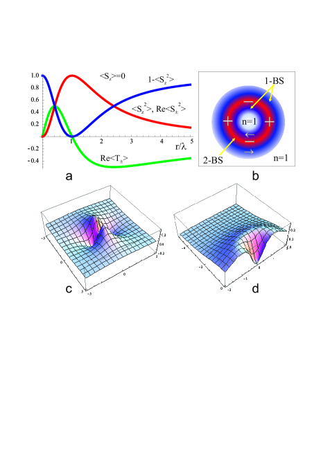
Fig.2 demonstrates the radial distribution of different (pseudo)spin order parameters for the quadrupole skyrmion. We see a circular layered structure with clearly visible anticorrelation effects due to a (pseudo)spin kinematics. Interestingly, at the center () and far from the center () for such a skyrmion we deal with a = 0, or Mott insulating state while for the domain wall center () we arrive at a = 1 superposition with maximal value of the parameter whose weight diminishes with moving away from the center. The parameter turns into zero at the domain wall center , at the skyrmion center and at the infinity (), with the two extremes at . In other words, we arrive at a very complicated interplay of single and two boson superfluids with density maxima at and at the domain wall center (), respectively. The ring shaped domain wall is an area with a circular distribution of the superfluid order parameters, or circular ”bosonic” supercurrent. Nonzero -type order parameter distribution points to a circular ”one-boson” current with a puzzlingly opposite sign ( phase difference) of the parameter for ”internal” () and ”external” () parts of the skyrmion, while the parameter defines the two-boson, or dimer superfluid order. The specific spatial separation of different order parameters that avoid each other reflects the competition of different terms in (43). Given the simplest winding number we arrive at the or -wave (/ in-plane symmetry of the one-boson or dimer superfluid order parameters, respectively.
One of the most exciting features of the quadrupole skyrmion is that such a skyrmionic structure is characterized by an uniform distribution of the mean on-site boson density = =1 as = 0. In other words, the quadrupole skyrmionic structure and bare “parent” Mott insulating phase have absolutely the same distribution of the mean on-site densities. From the one hand, this point underlines an unconventional quantum nature of the quadrupole skyrmion under consideration, while from the other hand it makes the quadrupole skyrmion texture to be an “invisible being” for several experimental techniques. However, the domain wall center of the quadrupole skyrmion appears to reveal maximal values of the pseudospin susceptibility bubble . It means the domain wall appears to form a very efficient ring-shaped potential well for the boson localization thus giving rise to a novel type of a “charged” topological defect. In the framework of the pseudospin formalism the “charging” of a bare “neutral” skyrmion corresponds to a single-magnon = 1 (single particle) or a two-magnon = 2 (two-particle) dimer excitations. It is worth noting that for large negative the single-magnon (single-particle) excitations may not be the lowest energy excitations of the strongly anisotropic pseudospin system. Their energy may surpass the energy of a two-magnon bound state (bimagnon), or two-boson dimer excitation, created at a particular site. Thus we arrive at a competition of two types of “charged” quadrupole skyrmions with = 1 and = 2, respectively ( is a total number of bosons). Such a “charged” topological defect can be addressed to be an extended skyrmion-like mobile quasiparticle. However, at the same time it should’nt be forgotten that skyrmion corresponds to a collective state (excitation) of the whole system.
The boson addition or removal in the half-filled () boson system can be a driving force for a nucleation of a multi-center “charged” skyrmions. Such topological structures, rather than uniform phases predicted by the mean-field approximation, are believed to describe the evolution of the EBHM systems away from half-filling. It is worth noting that the multi-center skyrmions one considers as systems of skyrmion-like quasiparticles forming skyrmion liquids and skyrmion lattices, or crystals (see, e.g., Refs. Timm, ; Green, ).
V.2.3 Dipole-quadrupole (pseudo)spin skyrmions
In the continual limit for the Hamiltonian (44) can be transformed into the classical Hamiltonian of the fully -symmetric scale-invariant model which can be rewritten as follows Nadya :
| (49) |
where we have used the representation (6) and introduced . The topological solutions for the Hamiltonian (49) can be classified at least by three topological quantum numbers (winding numbers): phases can change by after the passing around the center of the defect. The appropriate modes may have very complicated topological structure due to the possibility for one defect to have several different centers (while one of the phases changes by given one turnover around one center , other phases may pass around other centers ). It should be noted that for such a center the winding numbers may take half-integer values. Thus we arrive at a large variety of topological structures to be solutions of the model. Below we will briefly address two simplest classes of such solutions. One type of skyrmions can be obtained given the trivial phases . If these are constant, the vector distribution (see (6)) represents the skyrmion described by the usual formula (39). All but one topological quantum numbers are zero for this class of solutions. It includes both dipole and quadrupole solutions: depending on selected constant phases one can obtain both ”electric” and different ”magnetic” skyrmions. The substitution leads to the electric skyrmion which was obtained above as a solution of more general SU(3)-anisotropic model. Another example can be . This substitution implies , and . Nominally, this is the in-plane spin vortex with a varying length of the spin vector
which is zero at the circle , at the center and at the infinity , and has maxima at . In addition to the non-zero in-plane components of spin-dipole moment this vortex is characterized by a non-zero distribution of (pseudo)spin-quadrupole moments. Here we would like to emphasize the difference between spin-1/2 systems in which there are such the solutions as in-plane vortices with the energy having a well-known logarithmic dependence on the size of the system and fixed spin length, and spin-1 systems in which the in-plane vortices also can exist but they may have a finite energy and a varying spin length. The distribution of quadrupole components associated with in-plane spin-1 vortex is non-trivial. Such solutions can be termed as ”in-plane dipole-quadrupole skyrmions”.
Other types of the simplest solutions with the phases governed by two integer winding numbers and are considered in Ref. Nadya, .
VI Conclusion
Pseudospin formalism is shown to constitute a powerful method to study complex phenomena in interacting quantum systems. We have focused here on the most prominent and intensively studied S=1 pseudospin formalism for extended bosonic Hubbard model with truncation of the on-site Hilbert space to the three lowest occupation states n = 0, 1, 2. The EHBM Hamiltonian is a paradigmatic model for the highly topical field of ultracold gases in optical lattices. At variance with standard EHBM Hamiltonian that seems to be insufficient to quantitatively describe the physics of bosonic systems the generalized non-Heisenberg effective pseudospin Hamiltonian, Eqs.(21)-(24) does provide a more deep link with boson system and physically clear description of ”the myriad of phases” from uniform Mott insulating phases and density waves to two types of superfluids and supersolids. The Hamiltonian could provide a novel starting point for analytical and computational studies of semi-hard core boson systems. Furthermore, we argue that the 2D S=1 pseudospin system is prone to a topological phase separation and address different types of unconventional skyrmion-like structures, which, to the best of our knowledge, have not been analysed till now. The structures are characterized by a complicated interplay of the insulating and the two superfluid phases with a single boson and boson dimers condensation, respectively. Meanwhile we discussed the skyrmions to be classical solutions of the continual isotropic models, however, this idealized object is believed to preserve their main features for strongly anisotropic (pseudo)spin lattice quantum systems. Strictly speaking, the continuous model is relevant for discrete lattices only if we deal with long-wavelength inhomogeneities when their size is much bigger than the lattice spacing. In the discrete lattice the very notion of topological excitation seems to be inconsistent. At the same time, both quantum effects and the discreteness of the lattice itself do not prohibit from considering the nanoscale (pseudo)spin textures whose topology and spin arrangement is that of a skyrmion skyrmion-cuprates ; skyrmion .
We thank Yu. Panov and V. Konev for useful discussions. This research was supported in part by the program 02.A03.21.0006 and RFBR Grant No. 12-02-01039.
References
- (1) M.P.A. Fisher et al., Phys. Rev. B 40, 546 (1989); Subir Sachdev, Quantum Phase Transitions (Cambridge Univ. Press) 2001; O. Dutta, M. Gajda, P. Hauke, M. Lewenstein, D.-S. Lühmann, B.A. Malomed, T. Sowiński, J. Zakrzewski, arXiv:1406.0181.
- (2) Kwai-Kong Ng and Min-Fong Yang, Phys. Rev. B 83, 100511(R) (2011).
- (3) Ehud Altman and Assa Auerbach, Phys. Rev. Lett. 89, 250404 (2002); Erez Berg, Emanuele G. Dalla Torre, Thierry Giamarchi and Ehud Altman, Phys. Rev. B 77, 245119 (2008); L. Mazza, M. Rizzi, M. Lewenstein, and J.I. Cirac, Phys. Rev. A 82, 043629 (2010).
- (4) T. Matsubara and H. Matsuda, Prog. Theor. Phys. 16, 569 (1956).
- (5) C.D. Batista, G. Ortiz, Adv. in Phys. 53, 1 (2004).
- (6) P. Jordan and E. Wigner, Zeitschrift für Physik, 47, 631 (1928).
- (7) T. Holstein and H. Primakoff, Phys. Rev. 58, 1098 (1940).
- (8) A.S. Moskvin, Phys. Rev. B 84, 075116 (2011).
- (9) A.S. Moskvin, J. Phys.: Condens. Matter 25, 085601 (2013).
- (10) D.A. Varshalovich, A.N. Moskalev, V.K. Khersonskii. Quantum Theory of Angular Momentum (World Scientific, Singapore, 1988).
- (11) N.A. Mikushina, A.S. Moskvin, Phys. Lett. A 302, 8 (2002); arXiv:cond-mat/0111201.
- (12) A. Knigavko, B. Rosenstein, Y. F. Chen, Phys. Rev. B 60, 550 (1999).
- (13) M. Blume, Phys. Rev. 141, 517 (1966); H.W. Capel, Physica (Utrecht) 32, 966 (1966).
- (14) J.E. Hirsch and S. Tang, Phys. Rev. B 40, 2179 (1989); J.E. Hirsch, in ”Polarons and bipolarons in high- superconductors and related materials”, eds E.K.H. Salje, A.S. Alexandrov and W.Y. Liang, Cambridge University Press, 1995, p. 234.
- (15) P. Sengupta and C.D. Batista, Phys. Rev. Lett. 98, 227201 (2007); J. Appl. Phys. 103, 07C709 (2008).
- (16) K. Wierschem, Y. Kato, Y. Nishida, C.D. Batista, P. Sengupta, Phys. Rev. B 86, 201108(R) (2012).
- (17) M.R.H. Khajehpour, Yung-Li Wang, and Robert A. Kromhout, Phys. Rev. B 12, 1849 (1975).
- (18) J. Oitmaa and C.J. Hamer, Phys. Rev. B 77, 224435 (2008); C. J. Hamer, O. Rojas, and J. Oitmaa, Phys. Rev. B 81, 214424 (2010).
- (19) R.S. Lapa, A.S.T. Pires, Journal of Magnetism and Magnetic Materials 327, 1 (2013); A.S.T. Pires, Solid State Communications152, 1838 (2012).
- (20) N. Papanicolau, Phys. Lett. A 116, 89 (1986); Nucl. Phys. 305, 367 (1988).
- (21) J. Sasaki, F. Matsubara, J. Phys. Soc. Jap., 66, 2138 (1997).
- (22) A.A. Belavin, A.M. Polyakov, JETP Lett. 22, 245 (1975).
- (23) A.B. Borisov, S.A. Zykov, N.A. Mikushina, and A.S. Moskvin, Physics of Solid State 44, 324 (2002).
- (24) Ar. Abanov, V.L. Pokrovsky, Phys. Rev. B 58, R8889 (1998); B.A. Ivanov, A. Y. Merkulov,V. A. Stephanovich, and C. E. Zaspel, Phys. Rev. B 74, 224422 (2006); E. G. Galkina, E. V. Kirichenko, B. A. Ivanov, and V. A. Stephanovich, Phys. Rev. B 79, 134439 (2009).
- (25) A.M. Perelomov, ”Generalized coherent states and their applications”, Springer-Verlag, Berlin, 1986.
- (26) R.A. Istomin, A.S. Moskvin, JETP Lett. 71, 338 (2000).
- (27) P.B. Wiegmann, Phys. Rev. Lett. 60, 821 (1988); B.I. Shraiman and E.D. Siggia, Phys. Rev. Lett. 61, 467 (1988); X.G. Wen and A. Zee, Phys. Rev.Lett. 61, 1025 (1988); S. Chakravarty, B.I. Halperin, and D.R. Nelson, Phys. Rev. B 39, 2344 (1989); P. Voruganti and S. Doniach, Phys. Rev. B 41, 9358 (1990); R.J. Gooding, Phys. Rev. Lett. 66, 2266 (1991); S. Haas, F.-C. Zhang, F. Mila, and T.M. Rice, Phys. Rev. Lett. 77, 3021 (1996).
- (28) E. C.Marino and M.B. Silva Neto, Phys. Rev. B 64, 092511 (2001); T. Morinari, Phys. Rev. B 65, 064513 (2002); T. Morinari, Phys. Rev. B 72, 104502 (2005); Z. Nazario and D.I. Santiago, Phys. Rev. Lett. 97, 197201 (2006);
- (29) I. Raicevic, D. Popovic, C. Panagopoulos, L. Benfatto, M.B. Silva Neto, E.S. Choi, and T. Sasagawa, Phys. Rev. Lett. 106, 227206 (2011).
- (30) A. Bogdanov and A. Hubert, J. Mag. Mag. Mat. 138, 255 (1994); U.K. Rossler, A. Bogdanov and C. Pfleiderer, Nature 442, 797801 (2006); N. Nagaosa and Y. Tokura, Nature Nanotechnology 8, 899 (2013).
- (31) A.S. Moskvin, I.G. Bostrem, and A.S. Ovchinnikov, JETP Lett. 78, 772 (2003); A.S. Moskvin, Phys. Rev. B 69, 214505 (2004).
- (32) Carsten Timm, S.M. Girvin, H.A. Fertig, Phys. Rev. B 58, 10634 (1998).
- (33) A.G. Green, Phys. Rev. B 61, R16299 (2000).