Radial dependence of line profile variability in seven O9–B0.5 stars

Abstract

Context. Massive stars show a variety of spectral variability: presence of discrete absorption components in UV P-Cygni profiles, optical line profile variability, X-ray variability, radial velocity modulations.

Aims. Our goal is to study the spectral variability of single OB stars to better understand the relation between photospheric and wind variability. For that, we rely on high spectral resolution, high signal-to-noise ratio optical spectra collected with the spectrograph NARVAL on the Télescope Bernard Lyot at Pic du Midi.

Methods. We investigate the variability of twelve spectral lines by means of the Temporal Variance Spectrum (TVS). The selected lines probe the radial structure of the atmosphere, from the photosphere to the outer wind. We also perform a spectroscopic analysis with atmosphere models to derive the stellar and wind properties, and to constrain the formation region of the selected lines.

Results. We show that variability is observed in the wind lines of all bright giants and supergiants, on a daily timescale. Lines formed in the photosphere are sometimes variable, sometimes not. The dwarf stars do not show any sign of variability. If variability is observed on a daily timescale, it can also (but not always) be observed on hourly timescales, albeit with lower amplitude. There is a very clear correlation between amplitude of the variability and fraction of the line formed in the wind. Strong anti-correlations between the different part of the temporal variance spectrum are observed.

Conclusions. Our results indicate that variability is stronger in lines formed in the wind. A link between photospheric and wind variability is not obvious from our study, since wind variability is observed whatever the level of photospheric variability. Different photospheric lines also show different degrees of variability.

1 Introduction

Massive stars are important objects for several fields of astrophysics. Due to their high temperature and large luminosity, they have powerful ionizing spectra that create H II regions. With their large initial mass, they are able to go beyond the fusion of carbon in their core, thus producing a large fraction of the elements heavier than oxygen and contributing to the chemical evolution of galaxies. They explode as core-collapse supernovae, leading to the formation of neutron stars and stellar black holes. They are also the precursors of long-soft gamma ray bursts (Woosley & Bloom, 2006).

One of the main characteristics of massive stars is their strong winds. Because of the large luminosity, a large number of photons can be absorbed or scattered through spectral lines in the outer layers of massive stars, leading to a radiative acceleration strong enough to generate an outflow: the radiatively driven stellar wind. A massive star can lose 90$\%$ of its mass through such a wind during its life (Maeder & Meynet, 2000). The rate of mass loss ranges from $10^{-9}$ to $10^{-4}$ M_⊙ yr^-1, depending on the evolutionary status and luminosity. The velocity at which this stellar wind is driven can reach 4000 km s^-1 in the most extreme cases. The amount of mechanical energy released by stellar wind over the lifetime of a massive star is similar to the energy produced by the final supernova. The consequence is that massive stars keep injecting energy in the interstellar medium, participating in the support of turbulence.

The process of acceleration through spectral line is intrinsically unstable. The resulting acceleration is directly related to the velocity gradient in the atmosphere. Hence, a slight increase of the velocity gradient leads to a stronger acceleration, which in turn increases the velocity gradient (Owocki & Rybicki, 1984). This instability produces fluctuations in the velocity structure of a massive star’s atmosphere (MacGregor et al., 1979; Owocki et al., 1988; Feldmeier, 1995). Due to mass conservation, these velocity fluctuations induce density variations. Since spectral lines are sensitive to both the velocity and density structure, they are also affected.

Spectroscopic variability is commonly observed in massive stars in general and O stars in particular. UV resonance lines of O supergiants sometimes show Discrete Absorption Components (DACs) corresponding to zones of over-absorption throughout the blueshifted absorption part of the P-Cygni profile (Kaper et al., 1996; Fullerton, 2011). They are usually attributed to the presence of large scale structures leading to optical depth enhancement. Such structures may be due to Corotating Interacting Regions (CIRs) born in the photosphere. CIRs are thought to be produced by surface brightness variations, leading to modulations of the launching velocity between adjacent surface regions and ultimately to interaction between slower and faster material. Due to rotation, CIRs may subsequently develop through a spiral pattern, explaining that DACs are observed to move out of P-Cygni profiles with time. Optical observations also show line profile variability in the strongest wind lines of O stars, especially H$\alpha$ (e.g. de Jong et al., 2001). Morel et al. (2004) reported H$\alpha$ variability in all their sample stars showing wind dominated lines. Markova et al. (2005) studied a sample of O supergiants and concluded that the detected H$\alpha$ variability was usually consistent with a model of broken shells for the atmosphere, at least for the stars with the strongest winds. Such a model is a way of representing the density fluctuations caused by the line driving instability. Lines formed closer to the photosphere also vary. Fullerton et al. (1996) conducted a survey of 30 O stars and detected variability in HeI 5876 and sometimes CIV 5802-5812 for 77% of their sample, indicating that spectroscopic variability is widespread among O stars even in the deepest parts of the atmosphere. Subsequent studies have revealed variability in both wind and photospheric lines of O stars (de Jong et al., 2001; Kaufer et al., 2002; Prinja et al., 2004, 2006).

Whether there is a direct causal link between photospheric, surface variability and wind variability is still a matter of debate. It is not clear if the line driving instability can act on its own, at rather large velocities, or if it is an amplifier of deeply seated variations. de Jong et al. (2001) investigated this question in the case of the O7.5III star $\xi$ Per, using UV and optical spectroscopy. Although variability was observed in photospheric and wind features, a direct link was not obvious because of the different timescales of these variations. Kaufer et al. (2006) reached similar conclusions for the B0.5Ib supergiant HD 64760, although part of the H$\alpha$ variability has a periodicity comparable to that of lines formed closer to the photosphere. On the theoretical ground, surface variability is expected if the star experiences non-radial pulsations, as is the case of several O stars (Smith, 1978; Kambe et al., 1990; Fullerton et al., 1991; de Jong et al., 1999; Degroote et al., 2010). Surface inhomogeneities, possibly caused by magnetic spots, could also trigger variability.

To further test this relationship between photospheric and wind variability, more spectroscopic time series of O stars are required. As many photospheric and wind lines as possible should be monitored in order to sample the transition region between the stellar surface and the wind-dominated atmosphere. The classical indicators are usually H$\alpha$ and He I 5876. In this study, we consider 10 additional lines probing the inner part of the wind, down to the photosphere. We report on the spectroscopic variability of seven late-O/early-B stars using high resolution, high signal-to-noise spectra. We quantify the degree of variability by means of the Temporal Variance Spectrum (TVS) analysis developed by Fullerton et al. (1996). We also model the average profiles with the atmosphere code CMFGEN. Based on the models, we constrain the line formation region of each line. We investigate the radial dependence of variability throughout the photosphere-wind transition region of the sample stars. Our spectroscopic analysis also provides the fundamental parameters of the sample stars.

The paper is organized as follows: we present the observations in Sect. 2; the line profile variability is presented in Sect. 3; we describe the modelling of the stars and the determination of the line formation region in Sect. 4; we discuss our results in comparison to previous studies in Sect. 5 and present our conclusions in Sect. 6.

2 Observations and data reduction

The sample stars were initially selected as part of a program aiming at searching magnetic fields in massive stars. They are bright enough to allow repeated and frequent observations on a two meter telescope. Previous variability in the giants and supergiants was used as a potential indication of magnetic field, based on previous detections (e.g. Donati et al., 2002, 2006). The dwarf stars were objects with very weak winds which, according to Martins et al. (2005) could be due to the presence of a magnetic field. We selected the stars with a sufficient number of spectra to allow a variability study. In total, seven O stars with spectral type from O9 to B0.5 and luminosity classes from V to Iab were chosen. None of them is a known binary.

We used the spectropolarimeter NARVAL mounted on the Télescope Bernard Lyot at the Pic du Midi observatory to obtain high signal-to-noise, high spectral resolution data (see Bouret et al., 2008; Martins et al., 2010). The observations were obtained between October 16^th and October 25^th 2007, in June 2008 and between July 20^th and August 4^th 2009. NARVAL provides échelle spectra between 3700 Å and 1.05 $\mu$m. The signal to noise ratio per 2.6km s^-1 resolution bin depends on weather conditions and wavelength but is always larger than 200. The resolving power is 65 000. Table 1 gives the journal of observations.

The data were automatically reduced on site by the Libre Esprit software, a fully automatic reduction package for NARVAL data. Ample details on the reduction process can be obtained in Donati et al. (1997) and we refer the reader to this paper for information.

3 Line profile variability

To study the spectral variability of our sample stars, we have computed the Temporal Variance Spectrum (TVS) first introduced by Fullerton et al. (1996) and defined as follows:

$$TVS=\frac{1}{n-1}\sum_{i=1}^{n}\frac{w_{i}}{F_{i}}(F_{i}-F_{av})^{2}$$ (1)

where $F_{i}$ is the rectified flux, $F_{av}$ the mean rectified flux, $n$ the number of spectra available and $w_{i}$ a weighting factor taking into account the variation of the signal-to-noise ratio from spectrum to spectrum (see Eq. 11 of Fullerton et al., 1996). Given the relatively large exposure time, we have assumed that the photon noise was the main source of noise, implying that the factor $\alpha_{ij}$ of Fullerton et al., encompassing the wavelength dependence of noise, is equal to the flux $F_{i}$. The TVS is computed at all wavelengths and quantifies the degree of variability in a series of spectra. We have checked the effect of normalization uncertainties on the resulting TVS. One of us has normalized the same spectrum five times, and used the five resulting spectra to compute the TVS. The intensity we obtain is usually lower than 0.005, and is seen over the entire spectrum, not just in lines. We present two types of TVS depending on the data available: TVS computed for one night, when at least five spectra are available for the night; or TVS computed for several days. In the latter case, we use the average spectrum of the night (when several spectra are available) for each date.

We have selected twelve spectral lines to look for spectroscopic variability. In addition to the classical H$\alpha$ and He I 5876 features, we have added H$\beta$, H$\gamma$ which probe deeper layers than H$\alpha$ due to their reduced oscillator strength. We have also included three other He I lines (He I 4471, He I 4026 and He I 4712 in order of decreasing oscillator strength), three He II lines (He II 4542, He II 4686, He II 5412), O III 5592 and C IV 5802. The high ionization lines (C IV, He II, O III) probe deeper layers of the atmosphere compared to Balmer lines. The He I lines are triplets and belong to the 2p ³P^o series. With these lines, we are able to sample variability throughout the atmosphere of the sample stars.

We used continuum regions adjacent to the lines of interest to evaluate the one and three $\sigma$ levels. The one $\sigma$ level is set to the standard deviation around the mean value of the TVS in this continuum region.

3.1 Daily variability

In Fig. 1 we show the TVS and individual spectra of $\epsilon$ Ori between October 16^th and October 25^th 2007. We detect variability in all H and He I lines, as well as in He II 4686. The other He II lines, as well as O III 5592 and C IV 5802 do not show any significant variability. The shape of the TVS is similar in all lines for which variability is detected. There is a triple peak system, with the central peak being the strongest. It corresponds to variability in the line core. The two secondary peaks are located in the line wings, relatively far from the line core, at velocities up to 500 km s^-1 in H$\alpha$. Variability is usually larger and more extended in stronger lines. For example, the TVS reaches 0.042 in H$\alpha$, 0.024 in H$\beta$ and 0.020 in H$\gamma$. Variability extends up to 500 km s^-1 in H$\alpha$, 200 km s^-1 in H$\beta$ and 100 km s^-1 in H$\gamma$. The same trend of larger variability in stronger lines is seen in He I with the largest TVS maximum in He I 5876, then He I 4471, He I 4026 and He I 4712, corresponding to decreasing oscillator strength (see above).

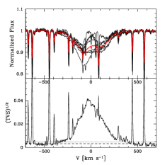
(a) H$\alpha$

(b) H_β

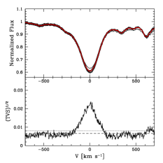
(c) H_γ

(d) He I 4026

(e) He I 4471

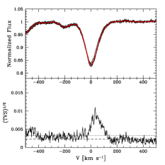
(f) He I 4712

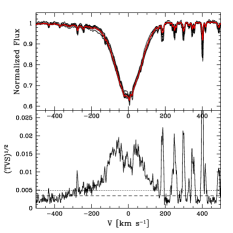
(g) He I 5876

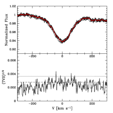
(h) He II 4542

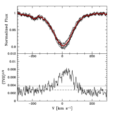
(i) He II 4686

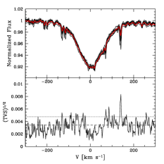
(j) He II 5412

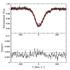
(k) O III 5592

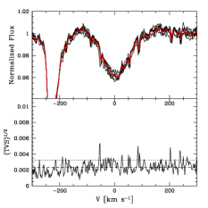
(l) C IV 5802

Figure 10: Variability of HD 167264 between July 25^th and August 4^th 2009.

We gather in Figs. 10 to 15 the same figures as Fig. 1 for the other sample stars. The variability of these stars is summarized as follows:

• HD 167264: this star shows variability in the same lines as $\epsilon$ Ori. The amplitude of the TVS is also of the same order (e.g. 0.04 for H$\alpha$). The shape of the TVS is mostly single peaked, except for He I 4026, He I 4471 and He I 5876 for which a double peak structure is observed.

• HD 207198: variability is observed in the H and He I lines, but also in all photospheric lines (He II, O III, C IV) although marginally in He II 4542. The shape of the TVS is mostly double peaked, as in HD 167264, with the red peak stronger than the blue one in the most strongly variable lines. In the He I lines, the amplitude of the blue peak in the TVS decreases with decreasing oscillator strength (it vanishes in He I 4712).

• HD 188209: it is variable in all lines, photospheric or wind dominated. The Balmer lines are mostly triple peaked, the red component being the strongest. The TVS of the He I lines is double peaked, with the red peak being usually stronger than the blue one. The high ionization lines (from C IV, O III, He II) are clearly variable.

• HD 209975: as in HD 188209, all lines are showing some degree of variability, with rather similar amplitudes. A double peak is seen in the TVS with an asymmetry red/blue, the red peak being stronger at least in the most variable lines.

• 10 Lac and AE Aur: both late O dwarfs do not show any evidence for variability in any of the lines. The spectra are very stable over several nights.

In general, we observe strong variability in giants/supergiants on a daily timescale. All low ionization lines (H I and He I) are variable. In two cases ($\epsilon$ Ori and HD 167264), the high ionization lines (He II, O III and C IV) are stable over days, while in the three other stars (HD 188209, HD 207198, and HD 209975) they also show clear changes from day to day. The former stars are B0-0.5 supergiants, while the latter are O9-9.5 supergiants. The two late-type O dwarfs (AE Aur and 10 Lac) do not show any variability on a daily timescale.

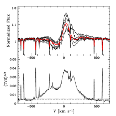
(a) H$\alpha$

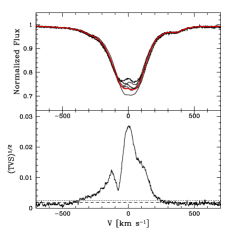
(b) H_β

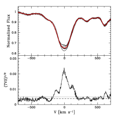
(c) H_γ

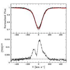
(d) He I 4026

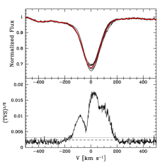
(e) He I 4471

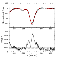
(f) He I 4712

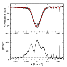
(g) He I 5876

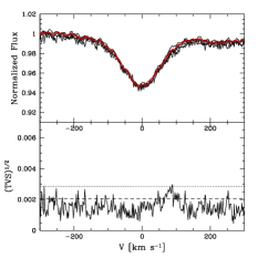
(h) He II 4542

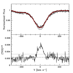
(i) He II 4686

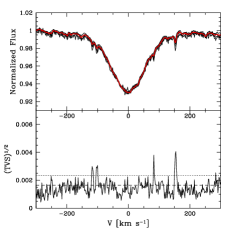
(j) He II 5412

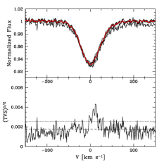
(k) O III 5592

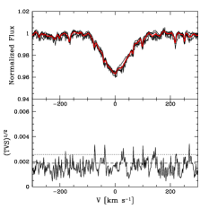
(l) C IV 5802

Figure 1: Variability of $\epsilon$ Ori on a daily timescale (from 16^th to 25^th October 2007). Upper panels: individual spectra in black (each spectrum corresponds to a night average) and global average spectrum in red. Lower panels: Temporal Variance Spectrum, together with the one sigma (dashed line) and three sigma (dot-dashed line) limits.

3.2 Hourly variability

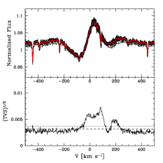
(a) H$\alpha$

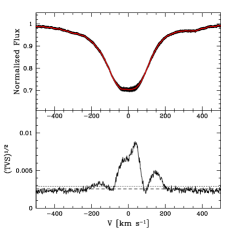
(b) H_β

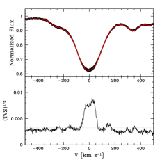
(c) H_γ

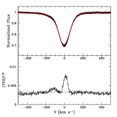
(d) He I 4026

(e) He I 4471

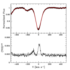
(f) He I 4712

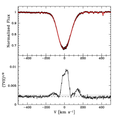
(g) He I 5876

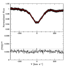
(h) He II 4542

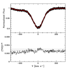
(i) He II 4686

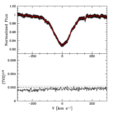
(j) He II 5412

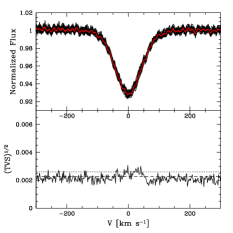
(k) O III 5592

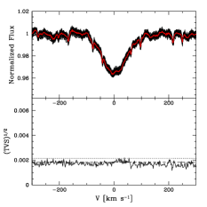
(l) C IV 5802

Figure 16: Variability of $\epsilon$ Ori on the night of 19^th to 20^th October 2007.

If we now look at Figs. 16 to 18, we see how the lines vary during a few hours (for the stars for which we have at least five spectra over a night).

• $\epsilon$ Ori: the changes during the night of October 19^th 2007 are shown. The amplitude is reduced compared to Fig. 1 (e.g. 0.008 instead of 0.042 for H$\alpha$) but the same lines show variability (and the same lines remain stable). Fig. 2 compares the TVS of the night of October 19^th 2007 to the TVS obtained on the night-averaged spectra over the October 2007 month, for the H$\alpha$ line. We see that on a timescale of hours, the variability is smaller than on a daily timescale. In addition, the strong variability observed over days extends up to 500 km s^-1 away from the line core. The shorter timescale variability is restricted to the line cores, either because the physical origin of this shorter timescale variability is different, or because the level of variability at high velocities is too small to be detected with our datasets. We have also computed the TVS during the night of October 22^nd and October 25^th 2007, but we did not detect any significant variability. The number of spectra available is much larger during the night of October 19^th, but if we compute the TVS using only a sample of six spectra taken during that night, the variability is still present. Thus, the lower number of spectra available for the night of October 22^nd and October 25^th does not explain the non detection of variability.

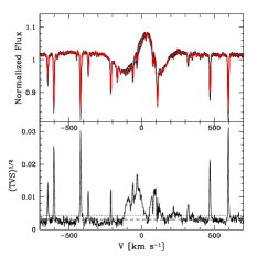
(a) H$\alpha$

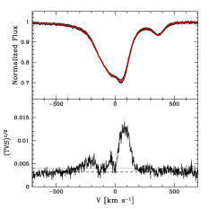
(b) H_β

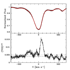
(c) H_γ

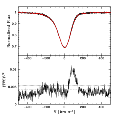
(d) He I 4026

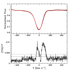
(e) He I 4471

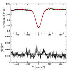
(f) He I 4712

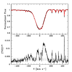
(g) He I 5876

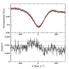
(h) He II 4542

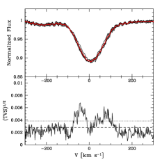
(i) He II 4686

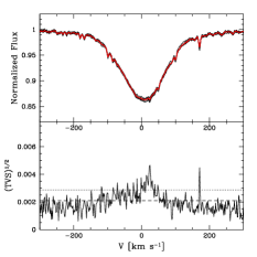
(j) He II 5412

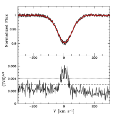
(k) O III 5592

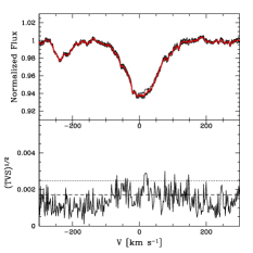
(l) C IV 5802

Figure 17: Variability of HD188209 during the night of June 25–26^th 2008.

• HD 188209: Fig. 17 reveals that HD 188209 is variable in all lines also on an hourly timescale during the night of June 25^th 2008. The variations in the high ionization lines are marginal. The variability is observed again during the night of June 27^th and 28^th 2008.

• HD 209975: during the night of June 28^th 2008, variability is observed in all lines except He II 4542 and C IV 5802. OIII 5592 is also very marginally variable. The variability is smaller than that observed on a daily timescale. The selected lines are also variable on the night of June 21^st, 22^nd and 27^th. The amplitude of the variations on June 21^st are smaller than on June 28^th, and only the most strongly variable lines are actually changing during that night. The time span of the observations is the same during all nights (about 2 hours).

The general conclusion is that stars showing variability on a daily timescale can also vary over a few hours. The variability on this shorter timescale is smaller (in intensity and velocity), and sometimes rescticted to the strongest wind lines. Conversely, if a line does not vary on a daily basis, it does not vary either on an hourly timescale. If the processes responsible for the daily and hourly variability are the same, then our observations indicate that the associated timescale is longer than days. However, if the processes are different, Fig. 2 suggests that the one acting on longer timescales leads to stronger variability than that acting on timescales of hours.

Figure 2: Daily and hourly H$\alpha$ TVS of $\epsilon$ Ori. The largest TVS is for the daily timescale. The hourly TVS is observed during the night of October 19^th 2007.

4 Spatial distribution of variability

4.1 Stellar and wind parameters

In order to better understand the origin of the observed variability, we have identified the line formation region for all features displayed in Fig. 1 and Figs 10 to 18. For that purpose, we have analyzed the spectroscopic data with atmosphere models computed with the code CMFGEN (Hillier & Miller, 1998). Our goal was to best reproduce the observed spectra to constrain the atmosphere structure and thus the line formation regions, directly accessible from the models. In practice, we have worked on the grand average of all optical spectra for each star. In order to constrain the wind structure, we also relied on far–UV spectra retrieved from the IUE archive. We used averaged spectra to have the highest possible signal-to-noise ratio, and to provide average parameters for the sample stars.

We used different diagnostics to compute the best fitting model for each star. In practice, we have proceeded as follows to determine those parameters:

• Effective temperature: we used the ionization ratio method to constraint T_eff. The He I and He II lines were the main indicators: He I 4026, He I 4388, He I 4471, He I 4712, He I 4920, He I 5876, He II 4200, He II 4542, He II 5412. He II 4686 is not considered since it also depends on the wind density.

• Gravity: the wings of the Balmer lines are the main diagnostics of $\log g$. They are broader at larger gravities. We used, H_β, H_γ, H_δ, H_ϵ, H I 3889 and H I 3835. The typical uncertainty on $\log g$ is 0.1 dex.

• Luminosity: we fitted the UV-optical-infrared SED to constrain the luminosity. When reliable (i.e. the uncertainty is lower than 30%), we used the Hipparcos parallaxes as constraints on the distances. The distances we used are reported in Table 2. We used the Galactic extinction law of Seaton (1979) and Howarth (1983) to constrain the extinction.

• Surface abundances: C and N abundances have been derived using the numerous carbon and nitrogen lines present in the optical range. C III 4070, C III 4153-56-63, C III 4326, C III 5305, C III 6205 were the main carbon abundance indicator. For nitrogen, we used N II 3995, N II 4041, N III 4196, N III 4216, NII 4447, N III 4511, N III 4515, N III 4523, N III 4602, NII 4607, NII 4621, N III 4907, N II 5676, N II 5679.

• Mass loss rate: the mass loss rate was determined from the strength of the UV P–Cygni lines (C III 1176, N V 1238-1242, C III 1247, Si IV 1393–1403, C IV 1548–1550) and from H_α. The typical uncertainty on $\dot{M}$ is 0.2 dex.

• Wind terminal velocity: $v_{\infty}$ was directly measured from the blueward extinction of the UV P–Cygni profiles. A typical uncertainty of 100km s^-1 is achieved.

• Clumping: clumping is treated by means of an exponential law in CMFGEN, where the volume filling factor $f$ has the following dependence on velocity: $f=f_{\infty}+(1-f_{\infty})e^{-\frac{v}{v_{cl}}}$. $f_{\infty}$ is the maximum clumping factor at the top of the atmosphere, and $v_{cl}$ determines the velocity at which clumping becomes non negligible. We adopted $v_{cl}$=30 km s^-1 and we derived $f_{\infty}$ from the shape of NIV 1720 line (Bouret et al., 2005).

• velocity slope: we constrained the slope of the velocity field - the so-called $\beta$ parameter - from the condition that both H$\alpha$ and the UV lines should be fitted for the same mass loss rate. Increasing the value of $\beta$ allows to reproduce the emission peak sometimes observed at the core of the broader H$\alpha$ absorption. The UV P-Cygni profiles are usually reproduced simultaneously. For the almost pure photospheric H$\alpha$ profiles of AE Aur end 10 Lac, $\beta$ was adopted.

• rotational velocity / macroturbulence: we used the Fourier transform method (Simón-Díaz & Herrero, 2007) to constrain the projected rotational velocity ($V$ sin$i$). We relied on the averaged spectrum to benefit from the highest signal-to-noise ratio. We used He I 4712 and O III 5592 as diagnostics. Once the value of $V$ sin$i$ was estimated, we used synthetic spectra (from our private database) to determine the macroturbulent velocity. We approximated macroturbulence by a Gaussian broadening. We tested several values of v_mac to best reproduce the diagnostic lines, for the estimated $V$ sin$i$. The best fit (selected by eye) provided v_mac.

The internal velocity structure of the atmosphere was iterated: we first converged the populations, then computed the resulting radiative acceleration and included it in a solution of the hydrodynamical equation to obtain a new velocity field. The populations was then re-converged with this hydrodynamical structure and the process was iterated. After a couple of these hydrodynamical iterations, the structure was usually consistent with the radiative transfer solution, except around the sonic point where a discrepancy was still present. Once the model atmosphere was converged, we performed a formal solution of the radiative transfer equation adopting a microturbulent velocity ranging from 10 km s^-1 in the photosphere to 0.1 $\times$ $v_{\infty}$ in the outer atmosphere. The resulting spectrum was compared to the observed spectra to constrain the stellar and wind parameters. The results of the spectroscopic analysis are gathered in Tab. 2.

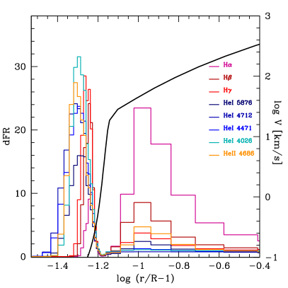
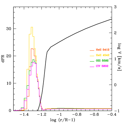
Figure 3: Formation region of lines shown in Figs. 1. The contribution function for a given line (in arbitrary units) is shown as a function of height above the photosphere. Left: lines showing variability in Fig. 1. Right: lines not showing variability in Fig. 1. The black solid line in both panels is the velocity structure in the best fit model.

4.2 Spatially resolved variability

Once a satisfactory fit was obtained, we retrieved the line formation region from the best fit model. The formation region is quantified by the contribution function, i.e. the fraction of the line produced as a function of radius. In Fig. 3, we show the formation region of the lines of $\epsilon$ Ori displayed in Fig. 1. The contribution function is evaluated at the line core. No correction for continuum has been performed, but we verified that the continuum just outside the line wings forms closer to the photosphere than the line core. We separate the lines showing variability (left panel) and the lines showing no variability at the 3$\sigma$ level (right panel). All lines are partly formed in the photosphere (i.e. below 10 km s^-1). The main difference between both sets of lines is that the variable lines have a significant contribution coming from high velocity, i.e. from the wind. This is clearly seen in H$\alpha$: the line is mainly formed between 1.1 and 1.25 R_star above the photosphere, which corresponds to velocities between 5 and 200 km s^-1. We thus conclude that the H$\alpha$ variability observed in Figs. 1 and 16 is rooted in the wind and not in the photosphere. More specifically, it is the inner part of the wind, at velocities of a few tens to a few hundreds of km s^-1, which is probed by H$\alpha$.

Using the best fit model for each star, we computed the fraction of the line formed above 10 km s^-1, i.e. in the wind part of the atmosphere. We did that for all lines. The choice of 10 km s^-1 is governed by the shape of the contribution function shown in Fig. 3. It corresponds to the velocity of the radius separating the two main peaks in the contribution function. A velocity of 10 km s^-1 is also close to the sonic point considered to be around the transition between the photosphere and the wind. Fig. 4 shows the intensity of the TVS as a function of the fraction of the line formed in the wind. We quantified the variability by the intensity of the TVS peak. We see a clear correlation: lines formed mostly in the wind are more variable than lines formed in the photosphere. The correlation is observed for all stars showing variability. This correlation between amplitude of variability and fraction of the line formed in the wind is valid for stars both showing and not showing changes in the photospheric lines. More specifically, the same level of H$\alpha$ variability is observed in $\epsilon$ Ori and in HD 188209. The former star show no sign of photospheric changes, while the latter is clearly variable in lines from high ionization states. It seems that the degree of variability in the photosphere is not directly correlated to the variability in the wind. This does not exclude a link between photospheric and wind changes in line profiles. But it suggests that instabilities in the wind can develop even if photospheric changes are absent (or at least weak).

Variability in lines formed mainly in the photosphere is quite complex. When present, variability is weaker than in wind lines. But lines formed at the bottom of the atmosphere do not behave similarly. For instance, the HeII and OIII lines in $\epsilon$ Ori do not vary while HeI 4026 and HeI 4713 do. All lines have very similar contribution functions (see Fig. 3). A similar behaviour is observed in HD 167264. This shows that the line formation position in the atmosphere is not the only parameter controlling line variability. For instance, Reid et al. (1993) suggested that for the fast rotator $\zeta$ Oph equator-to-pole temperature gradients lead to formation of He ii (He i) lines preferentially at the pole (equator). A latitudinal variation of the variability mechanism could then naturally explain the observed different behaviour of He i and He ii lines.

In Fig. 5 we show the effect of a variation of mass loss rate on the H$\alpha$ synthetic spectrum of $\epsilon$ Ori. The best fit model for $\epsilon$ Ori was used as a starting point. The TVS was computed assigning the same weight to all models. The mass loss rate varies by $\pm$25%. The associated TVS shows a single peak located close to the line core, slightly to its red side. The blue side of the TVS displays a shoulder. The TVS amplitude reaches 0.04, similar to what is observed in $\epsilon$ Ori. However, we do not observed the three peak structure in the TVS. In Fig. 6, the influence of a change in the velocity law slope ($\beta$) is shown. Here again, the best fit model for $\epsilon$ Ori is the starting point. $\beta$ is varied between 0.8 and 1.4. The TVS is strongly peaked around the line core, and is much narrower than the TVS resulting from changes in mass loss rates or the observed TVS. Its amplitude reaches a maximum of 0.15, much higher than what is observed for $\epsilon$ Ori.

The open black triangles in Fig. 4 correspond to the model shown in Fig. 5. A change in mass loss rate by 25% produces the same type of correlation between variability and fraction of line formed in the wind as what we observe for $\epsilon$ Ori (filled red triangles). The dotted triangles in Fig. 4 illustrate the effect of a variation of the slope of the velocity field (the $\beta$ parameter). We see that the same correlation is observed: the larger the fraction of the line formed in the wind, the stronger the variability. For the changes adopted ($\beta$ between 0.8 and 1.4) the variability of the lines with the smallest wind contribution is correctly reproduced, but the main wind lines show too strong variability compared to what is observed in $\epsilon$ Ori (field triangles).

The strongest variability in wind lines (quantified by the absolute value of the TVS maximum intensity) does not necessarily imply that the underlying mechanism responsible for the variability is stronger in the wind. Indeed, lines formed in the outer parts of the atmosphere are on average stronger (i.e. they have a larger oscillator strength) and form over wider regions. To first order, one expects a stronger reaction to any instability in stronger lines. To further investigate this issue, we computed the ratio of the maximum amplitude of the TVS divided by the line optical depth at the photosphere ($TVS^{peak}/\tau$), i.e. the depth at which the electron scattering optical depth is equal to 2/3. This is first order approximation to take into account line strength effects. The results are shown in Fig. 7. We see a different behaviour compared to Fig. 4: in all stars, there is a large scatter of $TVS^{peak}/\tau$ close to the photosphere and a decrease from the maximum value of $TVS^{peak}/\tau$ towards a minimum as the fraction of the line formed in the wind increases. Does this mean that the underlying variability mechanism is stronger close to the photosphere and that the stronger variability in lines formed mainly in the wind is only due to their higher strength and their formation over wider regions? Not necessarily either. Indeed, lines formed over a wide region may be subject to cancellation effects: variability at a given wavelength and a given position in the wind can be compensated by variability at another wavelength and another position corresponding to the same wavelength in the observer’s frame. Such cancellation effects are smaller in photospheric lines which all form in narrow regions.

Our investigations do not allow us to constrain the nature of the variability mechanism, nor its variation with depth. Nevertheless, we are able to show very clearly that there is a gradient of variability from the photosphere to the outer parts of the wind. Modulations in the wind parameters (mass loss rate, slope of the velocity field) can qualitatively explain the variability of the wind lines. We do not claim that true changes in the wind parameters are responsible for the observed variability. But the global density fluctuations they imply are qualitatively consistent with the observed line profile variations. In the photosphere, variability is quite complex and lines formed in very close regions may show different variability patterns.

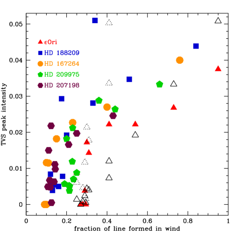
Figure 4: TVS peak intensity as a function of fraction of the line formed in the wind. Filled symbols correspond to the sample stars showing variability on a daily timescale. The solid open triangles show the variability of synthetic lines for which the mass loss rate varies by 25%, starting from the best fit model of $\epsilon$ Ori. The dotted triangles represent the theoretical variability due to changes in $\beta$ (from 0.8 to 1.4) in the best fit model of $\epsilon$ Ori. The points for H$\alpha$, H$\beta$ and H$\gamma$ are out of the plot (amplitude of 0.135, 0.104 and 0.070 respectively).

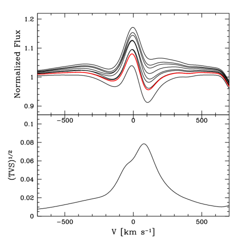
Figure 5: TVS of a serie of synthetic spectra computed from atmosphere models with $\dot{M}$ varying from 2.7 to 3.5 10^-6 M_⊙ yr^-1. The models are tailored to best represent the observed spectra of $\epsilon$ Ori.

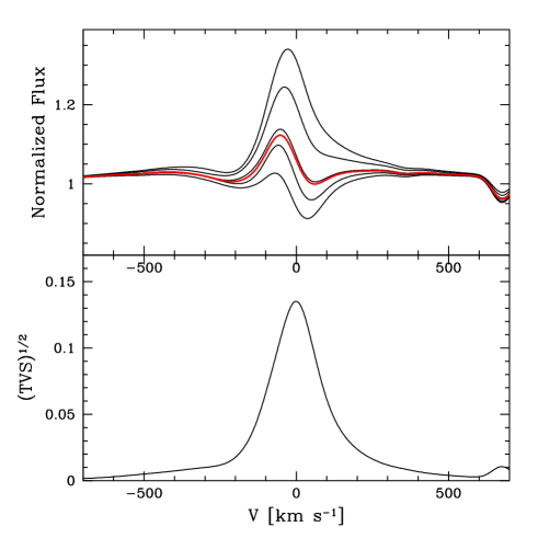
Figure 6: TVS of a serie of synthetic spectra computed from atmosphere models with $\beta$ varying from 0.8 to 1.4 for the case of $\epsilon$ Ori.

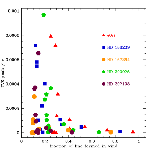
Figure 7: Same as Fig. 4 for the ratio of the TVS peak intensity to the line optical depth at the photosphere.

4.3 TVS profile

The TVS provides more information that the global level of variability. We illustrate this on the cases of $\epsilon$ Ori and HD 207198 which are typical of the types of variability observed: $\epsilon$ Ori does not show photospheric variability on the timescales we probe, while HD 207198 does. Both stars show wind line variability.

We use the autocorrelation function to extract information on the line profile variability. It is defined as

$$A(j,k)=\frac{\Sigma(s(j,l)\times s(k,l))}{\sqrt{(\Sigma s^{2}(j,l))\times(\Sigma s^{2}(k,l))}}$$ (2)

where $s(j,l)$ is the l^th spectrum at wavelength $j$. The $l$ index in the sum has been dropped for clarity. For a perfect (anti-) correlation between wavelengths $j$ and $k$, $A(j,k)$ is equal to 1 (-1).

In the upper panels of Fig. 8 we show selected H$\alpha$ and H$\gamma$ spectra of $\epsilon$ Ori illustrating the autocorrelation quantified in the matrixes displayed in the bottom panels. The triple-peak structure observed in Fig. 1 is also seen in the autocorrelation matrixes. There is a clear anti-correlation between the variability of the line core and of the line wings. The core is stronger when the wings are weaker. This type of anti-correlation is seen in all lines showing the triple peak structure. A profile showing regular core strengthening and line narrowing could account for such a behaviour. For instance, a change in the line broadening caused by a variable macroturbulence could explain such a behaviour. We simulated such a change by varying the macroturbulent velocity between 50 and 75 km s^-1 and we could reproduce a triple peaked structure in the TVS as well as the associated anti-correlation. One can also think of an extra emission on top of a photospheric profile. It could be caused by a shell of material initially just above the photosphere. At first, it would contaminate only the line core, making the overall profile less strong than a pure photospheric profile. The shell could subsequently expand, reaching larger velocity. The emission would then be spread over a range of velocities, and would consequently contaminate more the wings and less the line core. In that case the core would be stronger and the wings weaker than when the shell was just above the photosphere. This could reproduce the anti-correlation observed in $\epsilon$ Ori.

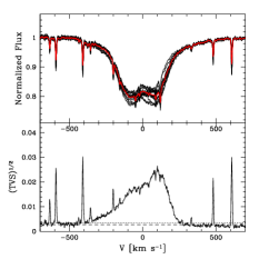
(a) H$\alpha$

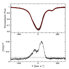
(b) H_β

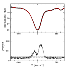
(c) H_γ

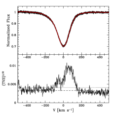
(d) He I 4026

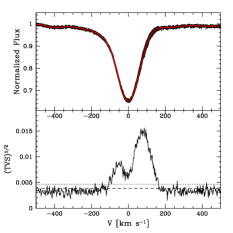
(e) He I 4471

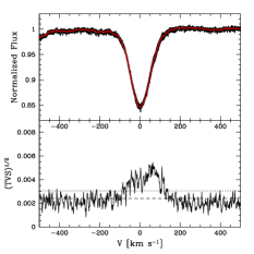
(f) He I 4712

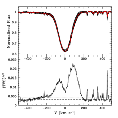
(g) He I 5876

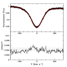
(h) He II 4542

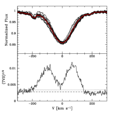
(i) He II 4686

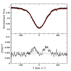
(j) He II 5412

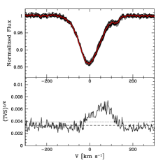
(k) O III 5592

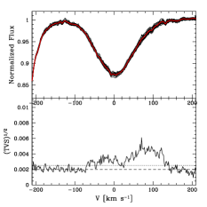
(l) C IV 5802

Figure 11: Variability of HD207198 between July 25^th and August 4^th 2009.

Fig. 9 shows the correlation matrixes and selected spectra for HD 207198. This star shows mainly double peaked structures in its TVS (see Fig. 11). The H$\alpha$ and H$\gamma$ lines show a clear anti-correlation between their blue and red wings. One possibility to explain such a behaviour is a simple radial velocity shift. But since not all lines show variability, we can exclude a bulk motion of the star. In addition, the two peaks are not always of the same strength, which is inconsistent with a radial velocity modulation. A moving shell does not account for the observed anti-correlation of the red and blue wings (see above). An asymmetry between the blue and red TVS peak can be explained by some types of wind asymmetries. For instance, Markova et al. (2005) performed simulations of clumpy winds with broken shells (see their Fig. 10). The resulting TVS is asymmetric, but with a stronger blue peak, contrary to what we observe. Their simulations of winds with a spiral pattern yield a symmetric TVS. The presence of blue and red variability could be explained in the case of winds confined by a magnetic field. Simulations by ud-Doula et al. (2013) show that if the star is not rotating too fast, material channelled along the field lines can settle in a disk-like structure and episodically fall back onto the star. Material reaching the equatorial plane at larger distance or flowing away from the surface at the poles can escape the star. This can qualitatively explain blue and red variability. However, since both infall and ejection of material happen at the same time, no anti-correlation is expected. In addition, no magnetic field has been detected on HD 207198. In Fig. 11 we see that as we move from lines mainly formed in the wind to photospheric lines (e.g. He II 5412) the asymmetry of the TVS disappears. This implies that any mechanism leading to this asymmetry is linked to the wind itself, and not to the photosphere.

In conclusion, the TVS shapes are complex and vary from star to star. But a qualitative interpretation indicates the important role of the wind to produce the observed structures, in agreement with the conclusions regarding the degree of variability (see Sect. 4.2).

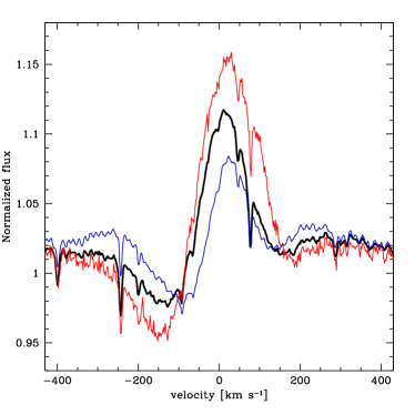
(a) H$\alpha$

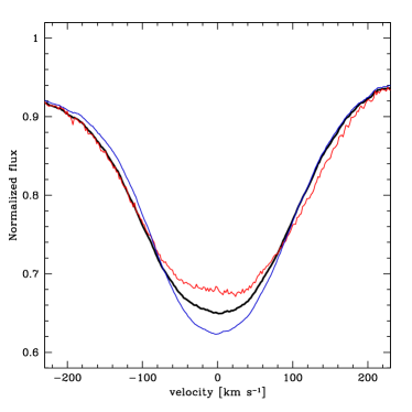
(b) H$\gamma$

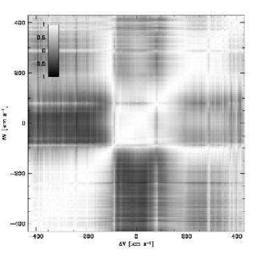
(c) H$\alpha$

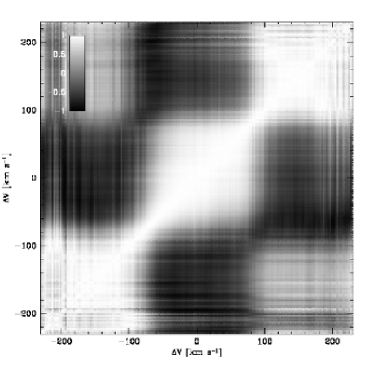
(d) H$\gamma$

Figure 8: Top panels: Selected H$\alpha$ (left) and H$\gamma$ (right) spectra of $\epsilon$ Ori showing an anticorrelated variation (with the average spectrum in bold line). Bottom panels: Autocorrelation matrixes. White (black) corresponds to a full (anti-) correlation. Only the part of the spectrum showing variability on a daily timescale is displayed.

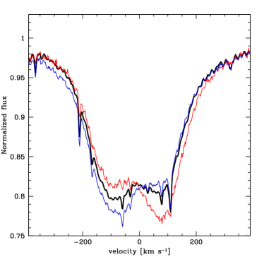
(a) H$\alpha$

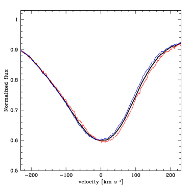
(b) H$\gamma$

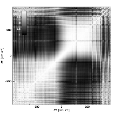
(c) H$\alpha$

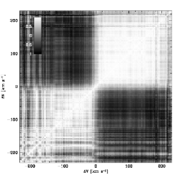
(d) H$\gamma$

Figure 9: Same as Fig. 8 for HD 207198.

5 Discussion

Several of our sample stars have been subject of variability study in the past.

Kaper et al. (1996) reported variability of 10 Lac in the bluest part of the N V 1238-1242 UV line, but not on all of their time series. No H$\alpha$ variability was detected by Kaper et al. (1997). 10 Lac was found to be a non-radial pulsator by Smith (1978). Our time series do not show any variability.

HD 188209 was studied by Fullerton et al. (1996). They gathered spectra over one night and detected variability in He I 5876 and C IV 5802. The variation they observe span the range [-200;100] km s^-1 about the line center. Our results obtained on the same timescale (night of 25-26 June 2008) are very similar, with variations in the range [-70;150] km s^-1. We also detect variability on June 27 and June 28. Markova et al. (2005) reported H$\alpha$ variability on a timescale of months. They concluded that changes in the mass loss rate by 17% could account for this variability. Israelian et al. (2000) reported variability with a period of 6.4 days that they tentatively attribute to binarity, although there are difficulties with this scenario (see their Sect. 7).

HD 209975 was also part of the sample of Fullerton et al. (1996). They collected spectra over one day and reported a variability of He I 5876 with an extension over $\pm$170 km s^-1. We also detect variability in He I 5876 on hourly timescale for all nights covered by our observations. The variability can be restricted to the first 100 km s^-1or extend up to 200 km s^-1 depending on the night, consistent with the findings of Fullerton et al. Markova et al. (2005) observed a monthly variability in H$\alpha$ that they could reproduce by 27% change in the mass loss rate of the star. Kaper et al. (1996) reported the presence of DACs in UV spectra of HD 209975, causing variations on a timescale of at leat 5 days. Subsequent observations in the UV and H$\alpha$ by Kaper et al. (1997) confirmed this timescale. The H$\alpha$ variability was found to extend over the first 200 km s^-1 around the line center. In our case, the TVS extends up to $\pm$300 km s^-1 on the timescale of the observations (7 nights).

$\epsilon$ Ori was observed by Prinja et al. (2004). Variability was detected in several lines, including H$\alpha$ and the weaker Si III 4553 feature. They highlighted a periodicity of 1.9 d in the variations of both the strong wind line H$\alpha$ and the Si III 4553, formed closer to the photosphere. They concluded that a direct link between photospheric and wind variability was revealed. Thompson & Morrison (2013) confirmed the presence of periodic signals on timescales of 2 to 7 days in both H$\alpha$ and He I 5876, which they interpreted as evidence for a connexion between photospheric and wind variability. Our results are consistent in the sense that we detect a clear variability in the wind lines. But we do not see any change in many photospheric lines (the He II, O III and C IV lines). We checked the behaviour of the Si III 4553 and detected a variability with a peak of the TVS of the order 0.010, in agreement with Prinja et al. (2004). As noted previously, some of the He I lines formed in the photosphere (He I 4026, He I 4713) do show variability, making the interpretation of the photospheric variability of $\epsilon$ Ori quite complex.
We investigated the presence of periodic signals in the variability we detect for $\epsilon$ Ori. We focused on H$\alpha$ since it is the most variable line, and we relied on its maximum emission as a proxy for our measurement. We performed a period search using the technique of Scargle (1982). We only detected a broad peak in the power spectrum at about 2 days. This is consistent with the findings of Prinja et al. (2004) and Thompson & Morrison (2013). However, our sampling is too coarse to get a good period identification.

Previous analysis were based on only a few lines (mainly H$\alpha$, He I 5876 and C IV 5802). Our study extends the investigation of the line profile variability to a much larger list of spectral features. We confirm that variability is mainly observed in wind sensitive lines. We show that there is a significant correlation between variability and fraction of the line formed in the wind. The question of whether these instabilities can be triggered by a photospheric mechanism or if they can be self-sustained is not settled. Our results indicate that some photospheric lines can be remarkably stable even if wind lines are variable. At the same time, different photospheric lines may be stable or not, as in the case of $\epsilon$ Ori or HD 167264. The effect of sub-surface convection in evolved massive stars (Cantiello et al., 2009) may explain the properties of stars showing photospheric variability, but fail to account for the objects without detectable variability or variability in only selected photospheric lines.

The presence of small scale magnetic loops could trigger magnetic activity close to the photosphere. This could be the seeds for wind variability (e.g. Fullerton et al., 1996; Morel et al., 2004). All our sample stars were initially part of a sample dedicated to the search for magnetic field among O stars. We did not detect any evidence for Zeeman signatures in the analysis of the spectro-polarimetric data, excluding strong magnetic field (B $>$ few 100 G, Grunhut et al. in prep.). In addition, all known O stars with a strong magnetic field show well defined rotational modulations (e.g. Donati et al., 2002, 2006; Wade et al., 2012) due to the presence of equatorial overdensities caused by magnetic wind confinment. In our sample stars, we detect variability on various timescales (hour-to-hour and night-to-night). This is not fully consistent with the presence of large scale magnetic field. However we cannot exclude much weaker fields of the order of a few Gauss (as discovered by Lignières et al. (2009) on Vega). Such fields could create surface inhomogeneities (temperature, composition) that might trigger photospheric variability subsequently amplified in the wind (e.g. by the line-driving instability). The photospheric variability could be weak so that we do not detect it in some of our sample stars.

Pulsations are also often claimed to be the seeds of spectral variability in OB-type stars. Kaufer et al. (2002) performed a large survey of the early B supergiant HD 64670 during 10 nights and reported the existence of periodic variability in photospheric lines. They could explain it by a model of stellar oscillations. Variability was also observed in H$\alpha$. Some of the features observed in this line could be assigned a periodicity similar to that of the photospheric lines. Some other patterns escaped this relation. Kaufer et al. (2002) concluded that there was a clear link between photospheric and wind variability. Prinja et al. (2006) studied the late-O supergiant $\alpha$ Cam. They reported hourly and daily variability in both H$\alpha$ and He I 5876. From the daily variability of He I 5876, they suggested that photospheric variations are present in the time serie analysis. In our analysis, we show that He I 5876 is one of the most variable line after the Balmer lines. In $\epsilon$ Ori, He I 5876 has a significant contribution from the wind (about 35%). Other lines are mainly photospheric (e.g. He II lines) and show no or weak variability. Hence in our sample stars, pulsations at the photosphere are difficult to relate to variability in lines formed further out in the wind, at least for stars without clear photospheric variability.

Line profile variability in OB stars is a complex process. Our results seem to indicate that a photospheric seed is not mandatory to trigger wind variability. However the behaviour of photospheric variability is difficult to interpret since lines formed over relatively similar regions, in the photosphere, may show different degrees of variability. In addition, the anti-correlations in the TVS are not easy to interpret. Dedicated simulations of specific variability mechanisms coupled to radiative trsnefer calculations are necessary to test possible excitation mechanisms.

Table 1: Physical parameters of the sample stars.

Star	ST	d	Teff	$\log\frac{L}{L_{\odot}}$	$\log g$	R	$V$ sin$i$	vmac	C/H	N/H	$\dot{M}$	$v_{\infty}$	$\beta$	f
		[pc]	[kK]			[R⊙]	[km s-1]	[km s-1]	[10-4]	[10-5]	[M⊙ yr-1]	[km s-1]
$\epsilon$ Ori	B0Iab	410$\pm$150	27.5$\pm$1.0	5.60$\pm$0.33	3.10	28.0$\pm$16.0	40	38	1.4$\pm$1.0	10.3$\pm$6.8	-6.25	1800	1.2	0.05
HD 167264	B0.5Ia/Iab	1700$\pm$510	28.0$\pm$1.0	5.65$\pm$0.27	3.10	28.6$\pm$12.5	70	22	1.2$\pm$0.5	18.0$\pm$8.0	-6.50	2000	1.8	0.1
HD 207198	O9II	620$\pm$180	32.5$\pm$1.0	5.05$\pm$0.26	3.50	10.6$\pm$4.4	60	27	1.6$\pm$0.8	20.0$\pm$6.0	-7.0	2000	3.0	1.0
HD 188209	O9.5Ib	2000$\pm$600	29.8$\pm$1.0	5.65$\pm$0.26	3.20	25.2$\pm$10.5	45	33	0.7$\pm$0.5	35.0$\pm$18.0	-6.4	2000	2.2	0.05
HD 209975	O9Ib	–	30.5$\pm$1.0	5.35$\pm$0.30	3.35	17.0$\pm$8.2	48	40	1.2$\pm$0.9	20.5$\pm$11.4	-6.50	2000	2.9	1.0
HD 34078	O9.5V	445$\pm$145	34.0$\pm$1.0	4.65$\pm$0.29	4.10	5.4$\pm$2.6	25	5	2.5$\pm$1.5	7.0$\pm$1.1	-10.0	1000	1.0	1.0
10 Lac	O9V	325$\pm$65	35.0$\pm$1.0	4.35$\pm$0.18	4.05	4.1$\pm$1.1	15	15	2.3$\pm$1.0	17.6$\pm$3.9	-9.70	1200	1.0	1.0

6 Conclusion

We have performed time series analysis of optical spectra of seven late-O early-B stars to investigate line profile variability. We have used spectra collected with the spectropolarimeter NARVAL mounted on the Télescope Bernard Lyot at Pic du Midi. The spectra have been obtained in several observing campaign between 2007 and 2009. Depending on the star, spectra have been collected over a single night or over several nights (sometimes with several exposures during individual nights). We have performed the analysis of the variability using the Temporal Variance Spectrum (TVS, Fullerton et al., 1996). We have also computed atmosphere models with the code CMFGEN to determine the fundamental properties of the sample stars, and to constrain the formation regions of the lines for which variability was investigated. Contrary to most previous studies, we did not restrict to lines formed in the wind, but we analyzed twelve spectral lines sampling the radial structure of the atmosphere. Our results can be summarized as follows:

• Variability is detected in the wind lines of all bright giants and supergiants. The dwarfs stars do not show any sign of line profile variability in any line.

• Photospheric variability in lines from high ionization states is sometimes observed, sometimes not, even if wind lines variability is definitely detected.

• In some cases the weakest photospheric He I lines may be variable even if the higher excitation lines are stable.

• When variability is detected on daily timescales, it is can also (but not always) be observed on hourly timescales, with a much lower amplitude.

• The shape of the temporal variance spectrum is usually double or triple peaked. Most of the double peaked structures show a red/blue asymmetry, the former being the strongest.

• Clear anticorrelations between these variable structures is observed.

• We find a clear correlation between amplitude of the variability and fraction of the line formed in the wind.

• There is no obvious relation between photospheric variability and stellar/wind parameters.

Our results are the first to provide variability information for a large sample of lines probing the entire radial structure of the atmosphere. They show for the first time a very clear correlation between the level of variability and the fraction of the line formed in the wind. At the same time, our results do not indicate that wind variability is always related to photospheric modulations.

Appendix A Journal of observations

In Table 1 we present the journal of observations for the target stars.

Table 2: Journal of observations. The signal to noise ratio (SNR) is given in the wavelength range 3800–6700 Å and depends on the exact wavelength.

Star	Date	HJD	exposure time	SNR
		[d]-2450000	[s]
$\epsilon$ Ori	16 oct 2007	4389.70536	40	150–600
(HD 37128)	18 oct 2007	4391.70278	60	150–650
	18 oct 2007	4391.70587	60	150–650
	18 oct 2007	4391.70896	60	150–650
	18 oct 2007	4391.71205	60	100–400
	18 oct 2007	4391.71516	60	100–350
	18 oct 2007	4391.71826	60	100–500
	19 oct 2007	4392.56330	180	150–900
	19 oct 2007	4392.56889	180	150–900
	19 oct 2007	4392.57334	180	150–900
	19 oct 2007	4392.57781	180	150–800
	19 oct 2007	4392.58228	180	200–950
	19 oct 2007	4392.58675	180	200–950
	19 oct 2007	4392.59121	180	200–1000
	19 oct 2007	4392.59574	180	200–950
	19 oct 2007	4392.60021	180	200–1000
	19 oct 2007	4392.60467	180	200–1050
	19 oct 2007	4392.60915	180	200–1100
	19 oct 2007	4392.61361	180	200–1100
	19 oct 2007	4392.61808	180	200–1100
	19 oct 2007	4392.62254	180	200–1000
	19 oct 2007	4392.62700	180	200–1050
	19 oct 2007	4392.63147	180	200–1100
	19 oct 2007	4392.63593	180	250–1200
	19 oct 2007	4392.64039	180	300–1300
	19 oct 2007	4392.64487	180	300–1300
	19 oct 2007	4392.64936	180	300–1300
	19 oct 2007	4392.65385	180	300–1300
	19 oct 2007	4392.65834	180	250–1200
	19 oct 2007	4392.66283	180	250–1200
	19 oct 2007	4392.66733	180	250–1150
	19 oct 2007	4392.67189	180	200–1100
	19 oct 2007	4392.67640	180	200–1000
	19 oct 2007	4392.68089	180	200–1000
	19 oct 2007	4392.68538	180	200–1000
	22 oct 2007	4395.71151	120	250–1300
	22 oct 2007	4395.71529	120	250–1250
	22 oct 2007	4395.71906	120	250–1200
	22 oct 2007	4395.72285	120	250–1250
	22 oct 2007	4395.72664	120	250–1200
	22 oct 2007	4395.73044	120	250–1200
	22 oct 2007	4395.73422	120	250–1200
	22 oct 2007	4395.73800	120	250–1200
	25 oct 2007	4398.71207	120	200–1100
	25 oct 2007	4398.71586	120	200–1100
	25 oct 2007	4398.71965	120	200–1000
	25 oct 2007	4398.72344	120	200–900
	25 oct 2007	4398.72723	120	200–900
	25 oct 2007	4398.73102	120	200–1000

Table 1: Continued

Star	Date	HJD	exposure time	SNR
		[d]-2450000	[s]
HD 188209	21 jun 2008	4639.45048	2700	100–600
	21 jun 2008	4639.48411	2700	100–500
	21 jun 2008	4639.51776	2700	100–600
	22 jun 2008	4640.45345	2700	200–1000
	22 jun 2008	4640.48707	2700	200–1000
	22 jun 2008	4640.52070	2700	200–1000
	25 jun 2008	4643.41578	2700	200–1000
	25 jun 2008	4643.44941	2700	200–950
	25 jun 2008	4643.48304	2700	200–900
	25 jun 2008	4643.51716	2700	200–900
	25 jun 2008	4643.55079	2700	200–900
	27 jun 2008	4645.39522	2700	200–1000
	27 jun 2008	4645.42886	2700	200–1100
	27 jun 2008	4645.46249	2700	200–1000
	27 jun 2008	4645.49613	2700	200–1100
	27 jun 2008	4645.52975	2700	200–1150
	28 jun 2008	4646.39664	2700	200–1100
	28 jun 2008	4646.43027	2700	200–1100
	28 jun 2008	4646.46391	2700	200–1100
	28 jun 2008	4646.49755	2700	200–1100
	28 jun 2008	4646.53120	2700	200–1050
	29 jun 2008	4647.59313	2700	200–1000
	29 jun 2008	4647.62682	2700	200–1050
	29 jun 2008	4647.66051	2700	200–1000
	30 jun 2008	4648.41724	2700	150–600
	30 jun 2008	4648.45106	2700	200–900
	30 jun 2008	4648.48536	2700	200–950
15 Sgr	25 jul 2009	5038.49492	2700	200–1000
(HD 167264)	26 jul 2009	5039.39600	2400	100–600
	27 jul 2009	5040.37934	2400	150–850
	28 jul 2009	5041.37153	2400	200–1000
	29 jul 2009	5042.37736	2400	200–1150
	31 jul 2009	5044.38242	2300	200–1100
	04 aug 2009	5048.43269	2300	200–900
HD 207198	24 jul 2009	5037.44575	2700	150–800
	25 jul 2009	5038.42181	2700	150–900
	25 jul 2009	5038.45546	2700	150–850
	27 jul 2009	5040.42000	2700	150–800
	27 jul 2009	5040.45362	2700	100–550
	28 jul 2009	5041.41078	2700	200–1000
	28 jul 2009	5041.44442	2700	200–1000
	29 jul 2009	5042.42667	2700	200–1050
	29 jul 2009	5042.46030	2700	200–1050
	30 jul 2009	5043.40589	2700	200–1000
	30 jul 2009	5043.43952	2700	200–1000
	31 jul 2009	5044.42425	2700	200–1100
	31 jul 2009	5044.45789	2700	200–1050
	01 aug 2009	5045.44377	2700	100–700
	04 aug 2009	5048.47207	2700	200–1000
HD 34078	15 oct 2007	4389.52124	2000	210–600
(AE Aur)	15 oct 2007	4389.59673	2000	300–750
	15 oct 2007	4389.62227	2000	300–800
	15 oct 2007	4389.64780	2000	300–800
	15 oct 2007	4389.67333	2000	300–800
	18 oct 2007	4392.46172	2000	200–600
	18 oct 2007	4392.48726	2000	200–550
	18 oct 2007	4392.51279	2000	200–560
	18 oct 2007	4392.53833	2000	130–370
	19 oct 2007	4393.49062	2000	320–830
	19 oct 2007	4393.51616	2000	310–810

Table 1: Continued

Star	Date	HJD	exposure time	SNR
		[d]-2450000	[s]
HD 209975	21 jun 2008	4639.54794	1800	300–800
	21 jun 2008	4639.57115	1800	280–700
	21 jun 2008	4639.59438	1800	280–680
	21 jun 2008	4639.61760	1800	380–900
	21 jun 2008	4639.64083	1800	350–850
	22 jun 2008	4640.55014	1800	500–1200
	22 jun 2008	4640.57336	1800	500–1200
	22 jun 2008	4640.59659	1800	550–1250
	22 jun 2008	4640.61983	1800	450–1150
	22 jun 2008	4640.64305	1800	400–1000
	25 jun 2008	4643.59284	1800	550–1250
	25 jun 2008	4643.61605	1800	550–1250
	25 jun 2008	4643.64215	1800	550–1350
	27 jun 2008	4645.56781	1800	650–1450
	27 jun 2008	4645.59102	1800	650–1450
	27 jun 2008	4645.61424	1800	650–1450
	27 jun 2008	4645.63782	1800	650–1450
	27 jun 2008	4645.66102	1800	650–1450
	28 jun 2008	4646.56284	1800	520–1250
	28 jun 2008	4646.58606	1800	470–1150
	28 jun 2008	4646.60928	1800	470–1180
	28 jun 2008	4646.63249	1800	570–1370
	28 jun 2008	4646.65571	1800	580–1400
HD 214680	15 oct 2007	4389.31523	1200	500–960
(10 Lac)	15 oct 2007	4389.33151	1200	550–1050
	15 oct 2007	4389.34780	1200	550–1050
	16 oct 2007	4390.41320	1200	520–1000
	16 oct 2007	4390.42949	1200	410–800
	16 oct 2007	4390.44577	1200	450–880
	17 oct 2007	4391.46364	2000	710–1410
	17 oct 2007	4391.48917	2000	700–1400
	17 oct 2007	4391.51470	2000	680–1380
	18 oct 2007	4392.25412	1200	400–800
	18 oct 2007	4392.27040	1200	360–720
	18 oct 2007	4392.28669	1200	340–680
	19 oct 2007	4393.26458	2000	620–1250
	19 oct 2007	4393.29011	2000	640–1280
	19 oct 2007	4393.31563	2000	660–1300
	20 oct 2007	4394.24877	2000	480–1200
	20 oct 2007	4394.27430	2000	680–1330
	20 oct 2007	4394.29984	2000	700–1360
	21 oct 2007	4395.26345	2000	500–1000
	21 oct 2007	4395.28899	2000	600–1200
	21 oct 2007	4395.31454	2000	640–1250
	23 oct 2007	4397.25262	2000	580–1170
	23 oct 2007	4397.27815	2000	580–1150
	23 oct 2007	4397.30369	2000	560–1340
	24 oct 2007	4398.25670	2000	640–1300
	24 oct 2007	4398.28224	2000	650–1300
	24 oct 2007	4398.30777	2000	750–1450

Appendix B Temporal variance spectra of sample stars

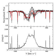
(a) H$\alpha$

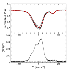
(b) H_β

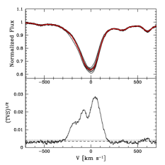
(c) H_γ

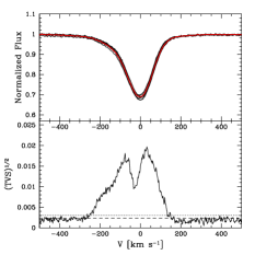
(d) He I 4026

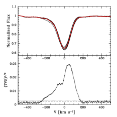
(e) He I 4471

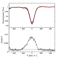
(f) He I 4712

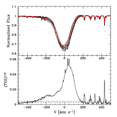
(g) He I 5876

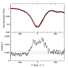
(h) He II 4542

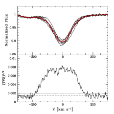
(i) He II 4686

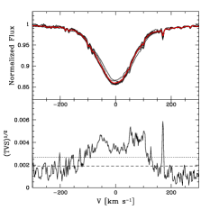
(j) He II 5412

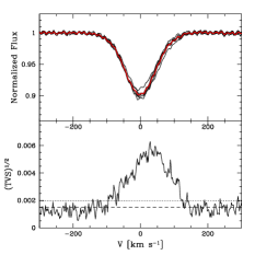
(k) O III 5592

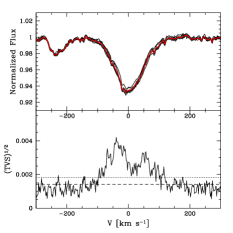
(l) C IV 5802

Figure 12: Variability of HD188209 between June 21^st and June 30^th 2008.

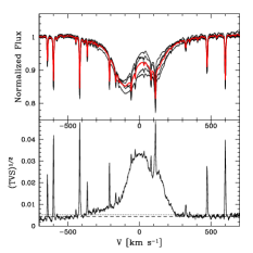
(a) H$\alpha$

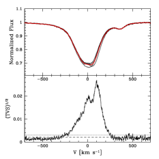
(b) H_β

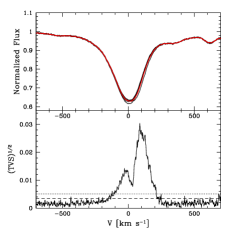
(c) H_γ

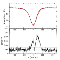
(d) He I 4026

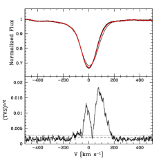
(e) He I 4471

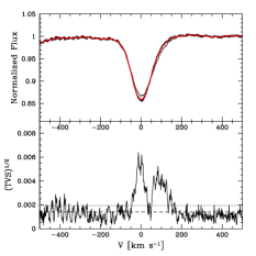
(f) He I 4712

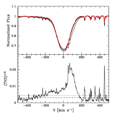
(g) He I 5876

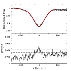
(h) He II 4542

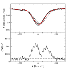
(i) He II 4686

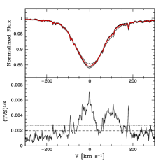
(j) He II 5412

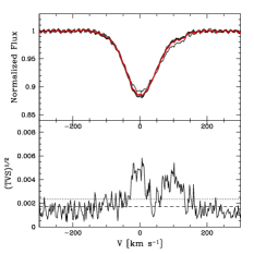
(k) O III 5592

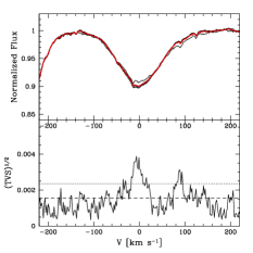
(l) C IV 5802

Figure 13: Variability of HD209975 between June 21^st and June 27^th 2008.

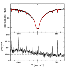
(a) H$\alpha$

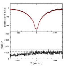
(b) H_β

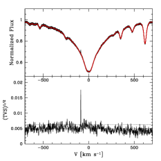
(c) H_γ

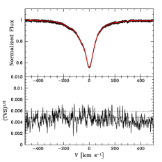
(d) He I 4026

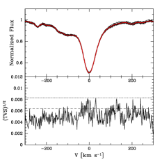
(e) He I 4471

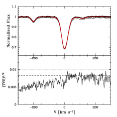
(f) He I 4712

(g) He I 5876

(h) He II 4542

(i) He II 4686

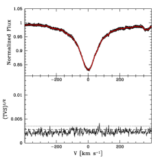
(j) He II 5412

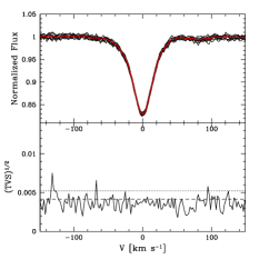
(k) O III 5592

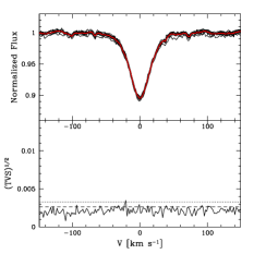
(l) C IV 5802

Figure 14: Variability of AE Aur between October 15^th and October 19^th 2007.

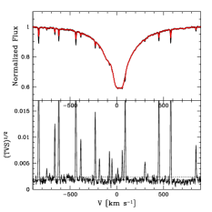
(a) H$\alpha$

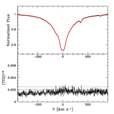
(b) H_β

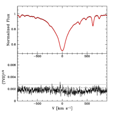
(c) H_γ

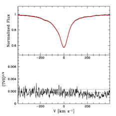
(d) He I 4026

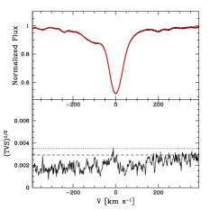
(e) He I 4471

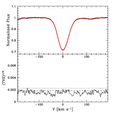
(f) He I 4712

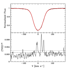
(g) He I 5876

(h) He II 4542

(i) He II 4686

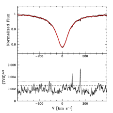
(j) He II 5412

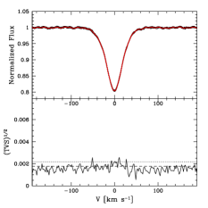
(k) O III 5592

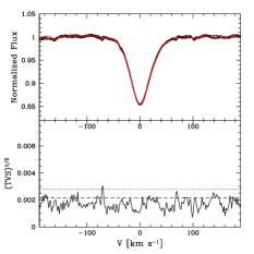
(l) C IV 5802

Figure 15: Variability of 10 Lac between October 15^th and October 24^th 2007.

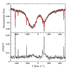
(a) H$\alpha$

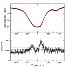
(b) H_β

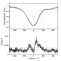
(c) H_γ

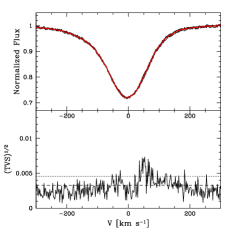
(d) He I 4026

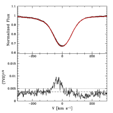
(e) He I 4471

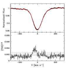
(f) He I 4712

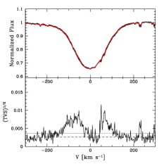
(g) He I 5876

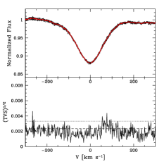
(h) He II 4542

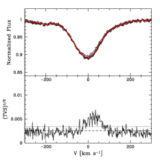
(i) He II 4686

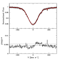
(j) He II 5412

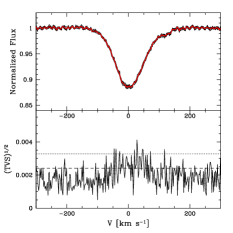
(k) O III 5592

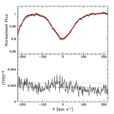
(l) C IV 5802

Figure 18: Variability of HD 209975 during the night of June 22^nd to 23^rd 2008.

Appendix C Best fits to the UV/optical spectra of the sample stars

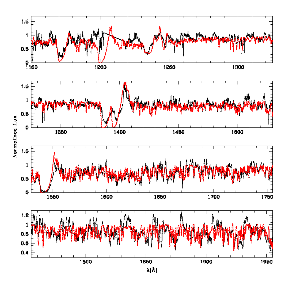
Figure 19: Best CMFGEN fit (red solid line) of the UV spectrum (black solid line) of $\epsilon$ Ori.

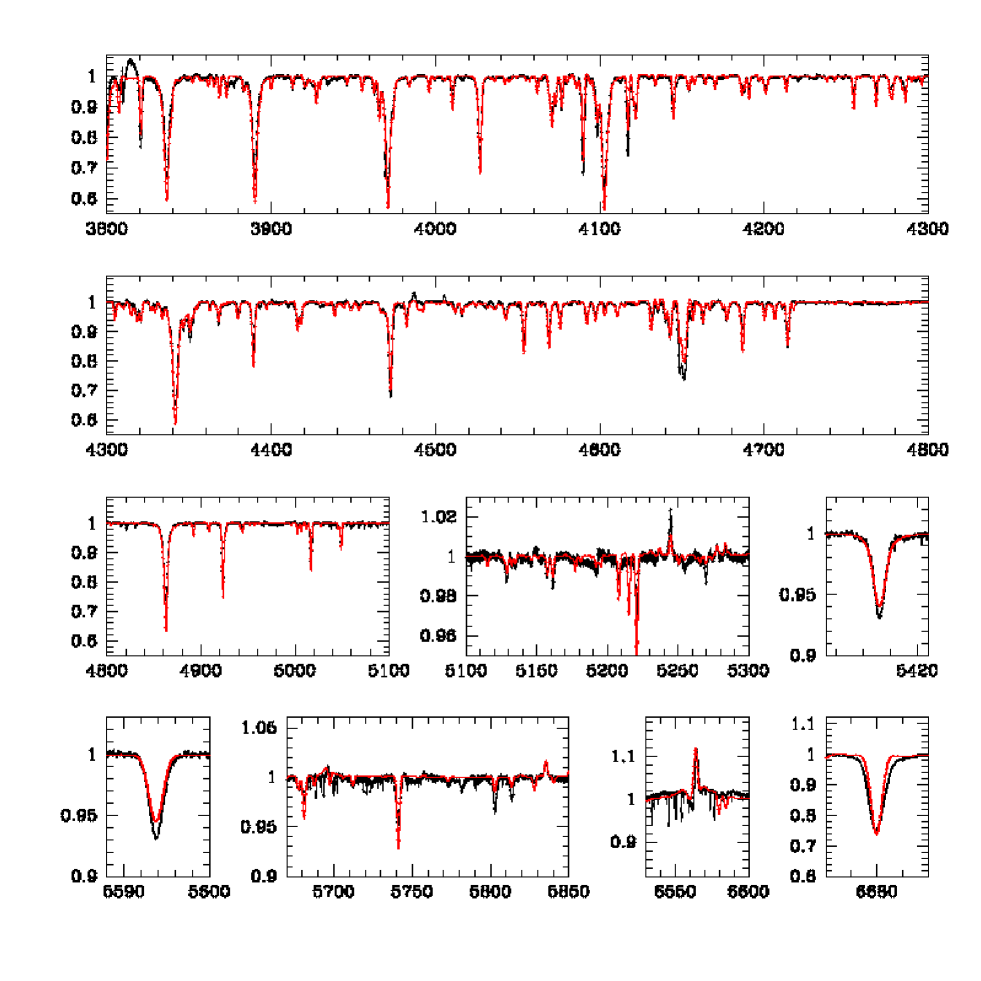
Figure 20: Best CMFGEN fit (red solid line) of the optical spectrum (black solid line) of $\epsilon$ Ori.

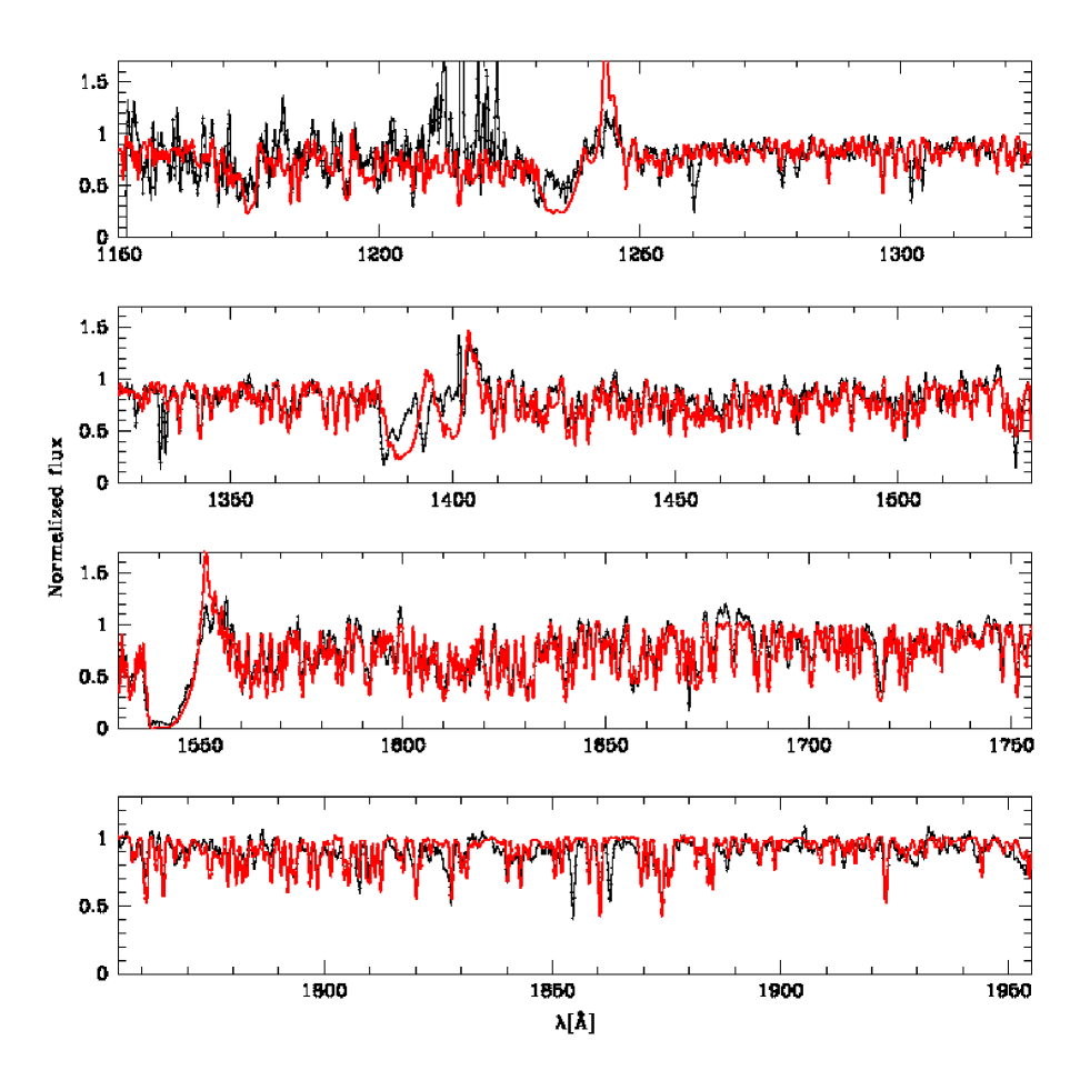
Figure 21: Best CMFGEN fit (red solid line) of the UV spectrum (black solid line) of HD 207198.

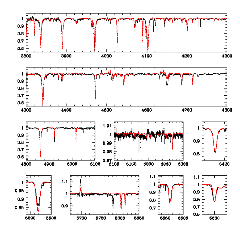
Figure 22: Best CMFGEN fit (red solid line) of the optical spectrum (black solid line) of HD 207198.

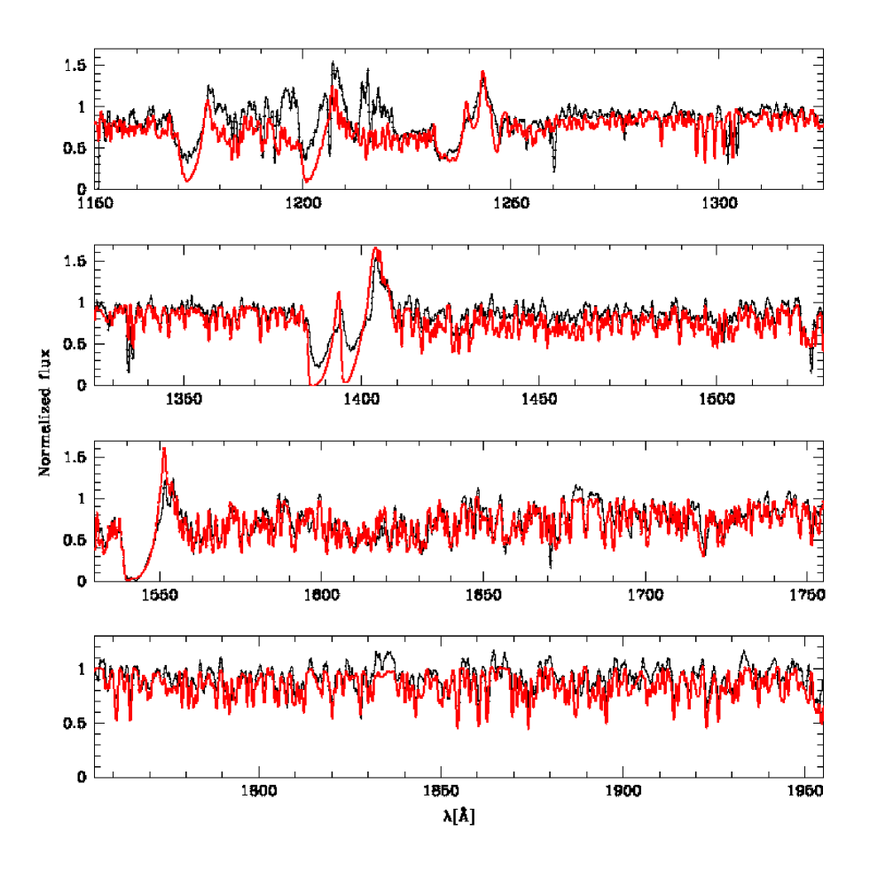
Figure 23: Best CMFGEN fit (red solid line) of the UV spectrum (black solid line) of HD 167264.

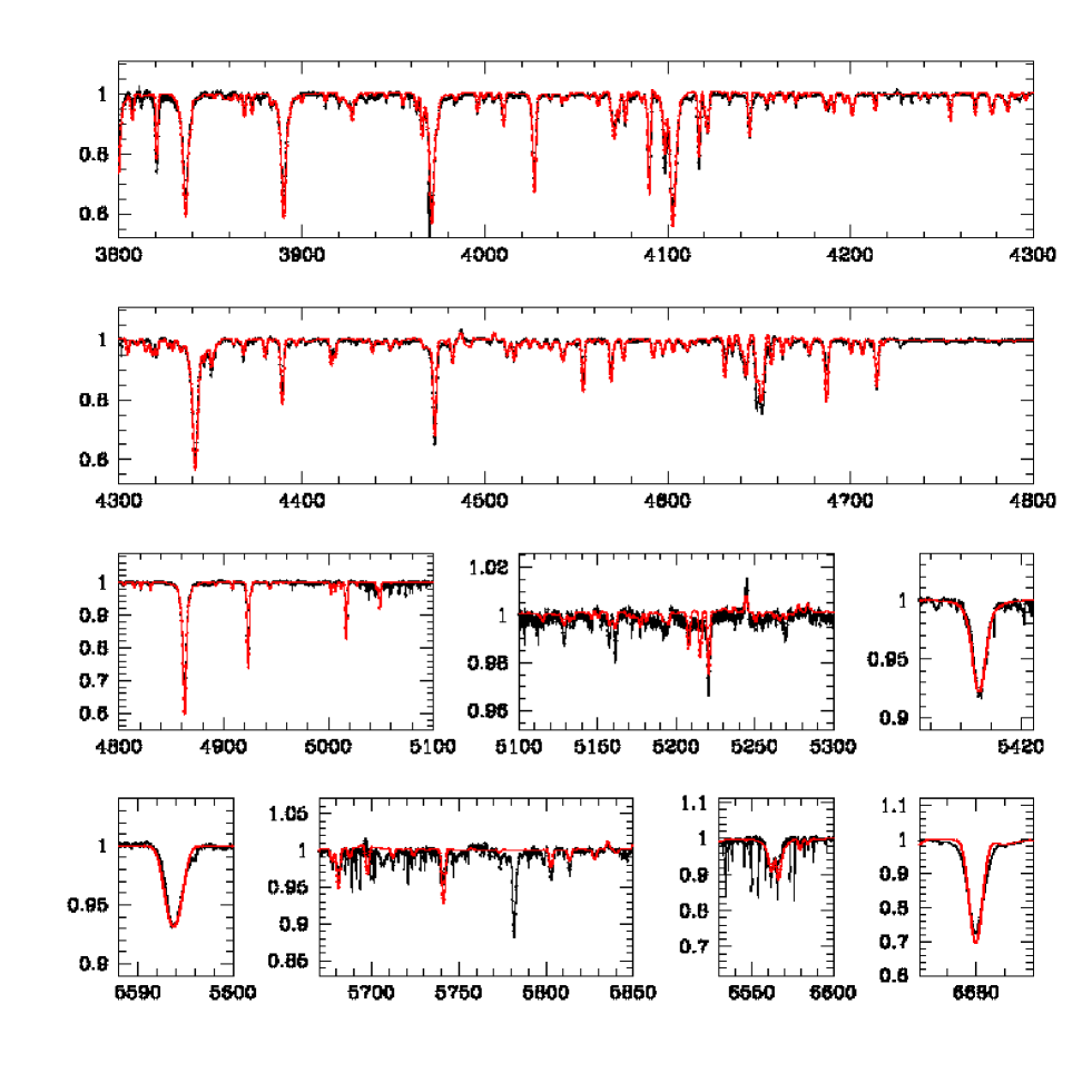
Figure 24: Best CMFGEN fit (red solid line) of the optical spectrum (black solid line) of HD 167264.

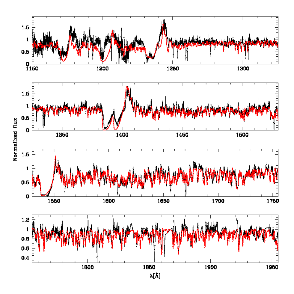
Figure 25: Best CMFGEN fit (red solid line) of the UV spectrum (black solid line) of HD 188209.

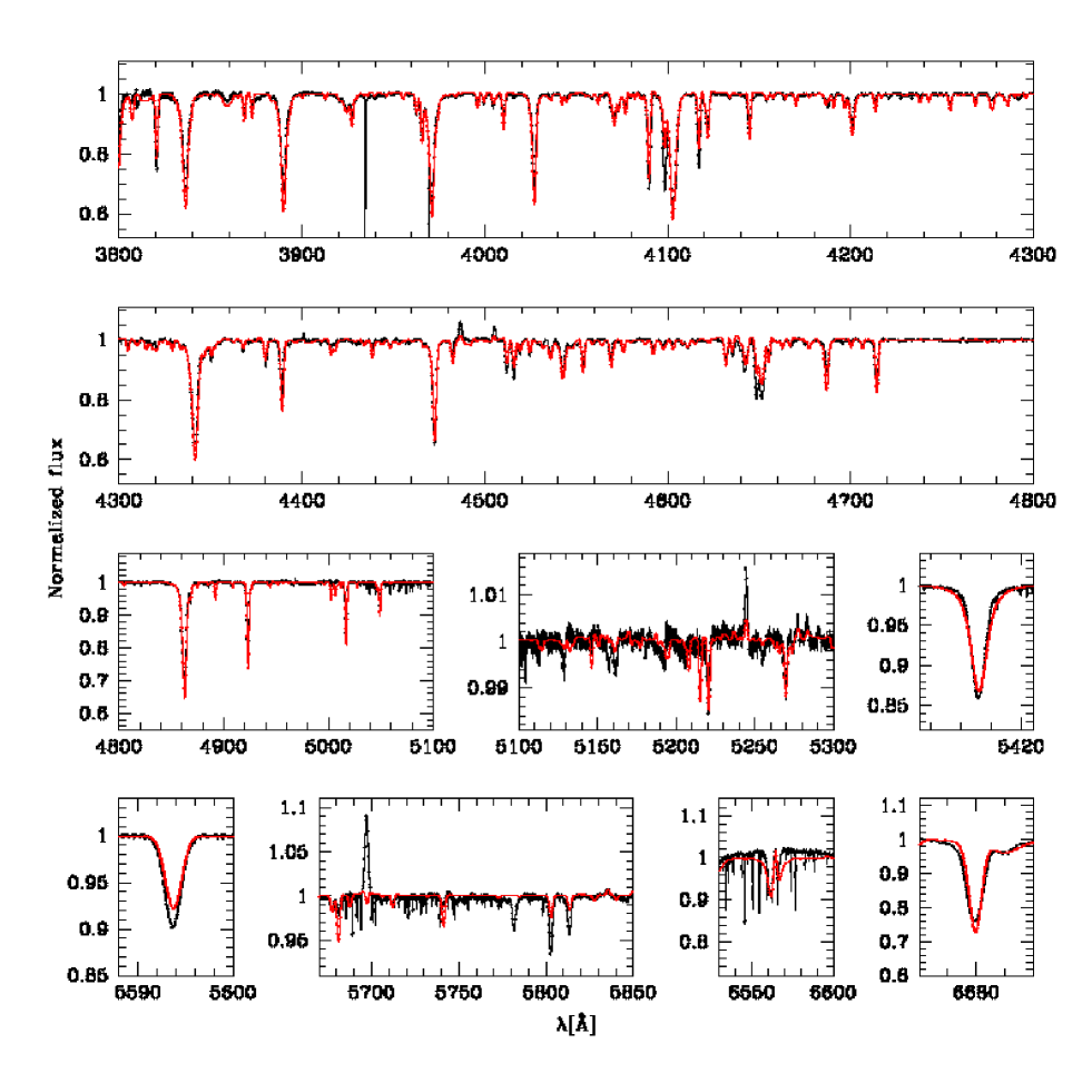
Figure 26: Best CMFGEN fit (red solid line) of the optical spectrum (black solid line) of HD 188209.

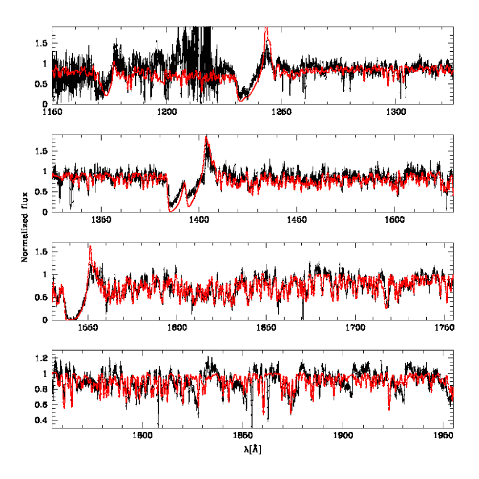
Figure 27: Best CMFGEN fit (red solid line) of the UV spectrum (black solid line) of HD 209975.

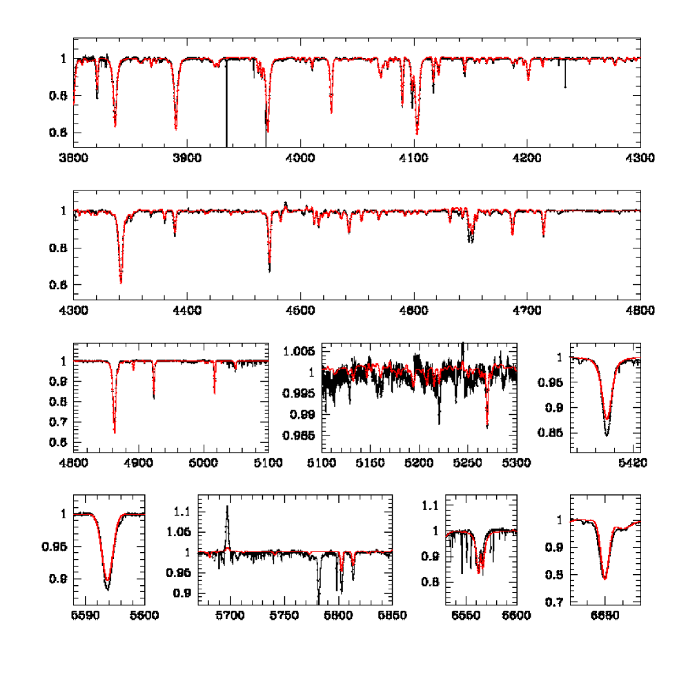
Figure 28: Best CMFGEN fit (red solid line) of the optical spectrum (black solid line) of HD 209975.

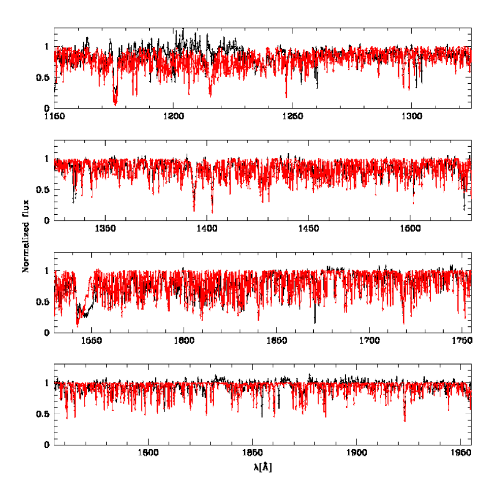
Figure 29: Best CMFGEN fit (red solid line) of the UV spectrum (black solid line) of 10 Lac.

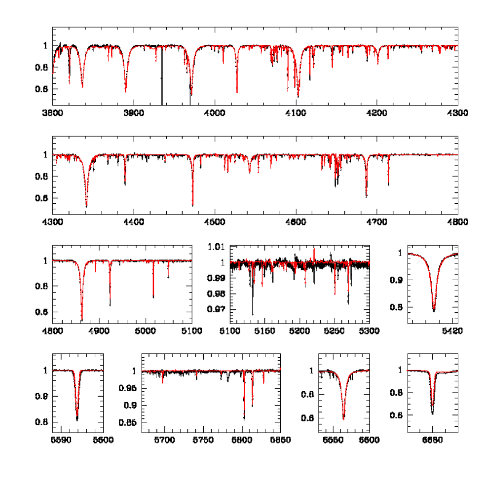
Figure 30: Best CMFGEN fit (red solid line) of the optical spectrum (black solid line) of 10 Lac.

Figure 31: Best CMFGEN fit (red solid line) of the UV spectrum (black solid line) of AE Aur.

Figure 32: Best CMFGEN fit (red solid line) of the optical spectrum (black solid line) of AE Aur.

References

- Bouret et al. (2008) Bouret, J.-C., Donati, J.-F., Martins, F., et al. 2008, MNRAS, 389, 75
- Bouret et al. (2005) Bouret, J.-C., Lanz, T., & Hillier, D. J. 2005, A&A, 438, 301
- Cantiello et al. (2009) Cantiello, M., Langer, N., Brott, I., et al. 2009, A&A, 499, 279
- de Jong et al. (2001) de Jong, J. A., Henrichs, H. F., Kaper, L., et al. 2001, A&A, 368, 601
- de Jong et al. (1999) de Jong, J. A., Henrichs, H. F., Schrijvers, C., et al. 1999, A&A, 345, 172
- Degroote et al. (2010) Degroote, P., Briquet, M., Auvergne, M., et al. 2010, A&A, 519, A38
- Donati et al. (1997) Donati, J., Semel, M., Carter, B. D., Rees, D. E., & Collier Cameron, A. 1997, MNRAS, 291, 658
- Donati et al. (2002) Donati, J.-F., Babel, J., Harries, T. J., et al. 2002, MNRAS, 333, 55
- Donati et al. (2006) Donati, J.-F., Howarth, I. D., Bouret, J.-C., et al. 2006, MNRAS, 365, L6
- Feldmeier (1995) Feldmeier, A. 1995, A&A, 299, 523
- Fullerton (2011) Fullerton, A. W. 2011, in IAU Symposium, Vol. 272, IAU Symposium, ed. C. Neiner, G. Wade, G. Meynet, & G. Peters, 136–147
- Fullerton et al. (1991) Fullerton, A. W., Gies, D. R., & Bolton, C. T. 1991, in Bulletin of the American Astronomical Society, Vol. 23, Bulletin of the American Astronomical Society, 1379
- Fullerton et al. (1996) Fullerton, A. W., Gies, D. R., & Bolton, C. T. 1996, ApJS, 103, 475
- Hillier & Miller (1998) Hillier, D. J. & Miller, D. L. 1998, ApJ, 496, 407
- Howarth (1983) Howarth, I. D. 1983, MNRAS, 203, 301
- Israelian et al. (2000) Israelian, G., Herrero, A., Musaev, F., et al. 2000, MNRAS, 316, 407
- Kambe et al. (1990) Kambe, E., Ando, H., & Hirata, R. 1990, in Lecture Notes in Physics, Berlin Springer Verlag, Vol. 367, Progress of Seismology of the Sun and Stars, ed. Y. Osaki & H. Shibahashi, 449
- Kaper et al. (1997) Kaper, L., Henrichs, H. F., Fullerton, A. W., et al. 1997, A&A, 327, 281
- Kaper et al. (1996) Kaper, L., Henrichs, H. F., Nichols, J. S., et al. 1996, A&AS, 116, 257
- Kaufer et al. (2002) Kaufer, A., Prinja, R. K., & Stahl, O. 2002, A&A, 382, 1032
- Kaufer et al. (2006) Kaufer, A., Stahl, O., Prinja, R. K., & Witherick, D. 2006, A&A, 447, 325
- Lignières et al. (2009) Lignières, F., Petit, P., Böhm, T., & Aurière, M. 2009, A&A, 500, L41
- MacGregor et al. (1979) MacGregor, K. B., Hartmann, L., & Raymond, J. C. 1979, ApJ, 231, 514
- Maeder & Meynet (2000) Maeder, A. & Meynet, G. 2000, ARA&A, 38, 143
- Markova et al. (2005) Markova, N., Puls, J., Scuderi, S., & Markov, H. 2005, A&A, 440, 1133
- Martins et al. (2010) Martins, F., Donati, J.-F., Marcolino, W. L. F., et al. 2010, MNRAS, 407, 1423
- Martins et al. (2005) Martins, F., Schaerer, D., Hillier, D. J., et al. 2005, A&A, 441, 735
- Mason et al. (1998) Mason, B. D., Gies, D. R., Hartkopf, W. I., et al. 1998, AJ, 115, 821
- Morel et al. (2004) Morel, T., Marchenko, S. V., Pati, A. K., et al. 2004, MNRAS, 351, 552
- Owocki et al. (1988) Owocki, S. P., Castor, J. I., & Rybicki, G. B. 1988, ApJ, 335, 914
- Owocki & Rybicki (1984) Owocki, S. P. & Rybicki, G. B. 1984, ApJ, 284, 337
- Perryman et al. (1997) Perryman, M. A. C., Lindegren, L., Kovalevsky, J., et al. 1997, A&A, 323, L49
- Prinja et al. (2006) Prinja, R. K., Markova, N., Scuderi, S., & Markov, H. 2006, A&A, 457, 987
- Prinja et al. (2004) Prinja, R. K., Rivinius, T., Stahl, O., et al. 2004, A&A, 418, 727
- Reid et al. (1993) Reid, A. H. N., Bolton, C. T., Crowe, R. A., et al. 1993, ApJ, 417, 320
- Scargle (1982) Scargle, J. D. 1982, ApJ, 263, 835
- Seaton (1979) Seaton, M. J. 1979, MNRAS, 187, 73P
- Simón-Díaz & Herrero (2007) Simón-Díaz, S. & Herrero, A. 2007, A&A, 468, 1063
- Smith (1978) Smith, M. A. 1978, ApJ, 224, 927
- Thompson & Morrison (2013) Thompson, G. B. & Morrison, N. D. 2013, AJ, 145, 95
- ud-Doula et al. (2013) ud-Doula, A., Sundqvist, J. O., Owocki, S. P., Petit, V., & Townsend, R. H. D. 2013, MNRAS, 428, 2723
- Wade et al. (2012) Wade, G. A., Grunhut, J., Gräfener, G., et al. 2012, MNRAS, 419, 2459
- Woosley & Bloom (2006) Woosley, S. E. & Bloom, J. S. 2006, ARA&A, 44, 507