A Unified Mathematical Language
for Medicine and Science

Abstract

A unified mathematical language for medicine and science will be presented. Using this language, models for DNA replication, protein synthesis, chemical reactions, neurons and a cardiac cycle of a heart have been built. Models for Turing machines, cellular automaton, fractals and physical systems are also represented with the use of this language. Interestingly, the language comes with a way to represent probability theory concepts and also programming statements. With this language, questions and processes in medicine can be represented as systems of equations; and solutions to these equations are viewed as treatments or previously unknown processes. This language can serve as the framework for the creation of a large interactive open-access scientific database that allows extensive mathematical medicine computations. It can also serve as a basis for exploring ideas related to what could be called metascience.

1 A Vision of Medicine

Imagine a world where treatments are computed and where knowledge of medicine is merged in a large database. New treatments are computed based on mathematical models built by researchers and each new model, like a piece of a puzzle, can be connected within a vast system of knowledge. Potential new treatments would be tested within a computational model and effects would be observed virtually, making animal experimentation obsolete due to lack of accuracy. New processes explaining functions of the body would be computationally deduced and hypothesized. Ultimately, treatments with minimal sides effects would be tailored to each patient based on their personal biological data.

It is difficult to keep up-to-date with new important research and publications and impossible to cover all the new daily literature in one’s domain of study. We are at a point where even a group of experts with the best communication tools and habits cannot efficiently integrate all the new knowledge of their field. In contrast, we now have the technological means to gather and analyse large amount of data.

A key component needed for the realization of this future is a common language for science and medicine. In this paper, we present a unified mathematical language which can be used to represent biological processes and scientific concepts. Although the examples are geared towards medicine, we will also present how this language can be used in different domains with the aim of demonstrating that effort in developing such a language can lead to improved communication and exchange of ideas between fields of studies.

Translating each research paper into a set of mathematical expressions and integrating it into a large database would ensure the findings of each new research study would be integrated into the existing body of knowledge. A feature of this language is that it could encompass the results of a vast number of papers, so that computations, discoveries and analysis could also be done on the field of medicine as a whole field. This could be a step into a new domain which could be called meta-medicine. This could be an opportunity to bridge the gap between publishing results and the integration of the results by the community. Competing theories and contradicting results could be tested against each other through computation and help to improve the general model. Interestingly, experimental results which are usually considered inconclusive or ‘negative’ could also contribute to enrich the global database.

2 Purpose of the Language

The objective behind these investigations is to build a language in which all scientific concepts and notations can be represented, while keeping the way each discipline functions and by enhancing the computational nature of each discipline. Along with the ability to represent all scientific concepts and its computational power, we would also need a language that allows navigation between different levels of complexity or scales (from DNA replication to body mechanics), can be used in a large database, has a visual notation and compact notation and has a relative ease of use regardless of the domain of study. With this language, dynamic models in biology, chemistry, neuroscience, computer science and physics have been built. We hope that sufficient steps have been taken towards demonstrating that the language has the qualities mentioned above and that this will inspire others to explore it further.

In mathematics, set theory combined with mathematical logic is known to be able to represent most mathematical expressions and concepts, but in practice we rarely directly use set theoretical expressions to represent or solve mathematical problems. Similarly, in computer science, although all programs can be reduced to Turing machines of zeros and ones, we rarely think or interact with high-level programming languages in this way. Whatever the language, there seems to be a gap between what we do in the discipline and the fundamental language. We could say that English along with all mathematical symbols is a complete language which can communicate any scientific concept, but unfortunately, computations cannot be done efficiently on words and sentences. The mathematical languages known as rewriting systems [Terese] are very powerful and have been shown to represent grammar, plants and fractals [Chomsky, Lindenmayer]. However, the scope of these systems is sometimes restricted to certain types of objects and focuses on automatic theorem proving, normal forms (expressions that cannot be transformed further) and termination.

The language which will be presented can be viewed as a higher order rewriting language that has no restrictions on the type of objects and on the objects that can be named. Alternatively, the language could be viewed as a higher order universal Turing machine where the symbols, states and tape can be any type of object. Furthermore, we could say that the head of the Turing machine could affect its own states and the symbols on the tape could also affect the states and properties of the head. Example of types of objects are models of atoms, molecules, DNA strands, cells, neurons, concepts, mathematical equations, programs, 3D geometrical structures, people and also infinite collections of different types of objects.

The driving question underlying this study can be written as:

What are the atoms of scientific concepts and how can we combine them to represent complex systems?

3 Essence of the Language

In this section, we introduce the elementary elements of the language. This is only meant to offer a quick glance at the language and one should read further in the subsequent sections for a more accessible and progressive description of the language along with key applications to biology, medicine and other scientific domains.

Everywhere we look in the world, we see change. We observe changes at every level, whether it be atoms, humans or the stars; they are changing all the time. As observers, we can take note of these changes and record them. Based on these records, we can infer and extrapolate the past and the future. In studying these records, we recognize interesting structures and name them. The principles behind the unified mathematical language that will presented can be reduced to the following two statements:

1. Observe a change in the world. Record what it was and what it became.

2. All objects and changes can be named.

For example, let $A$ and $B$ be objects. We will denote the transformation of object $A$ into $B$ by the notation

$$\framebox{$B\rhd A$}.$$

This notation should be understood as $B$ having the potential to slide down over the triangle $\rhd$ in the direction of $A$ so that $B$ will take the place of $A$. In itself, this object that we call a transformation is interesting, but it only represents a potential. For the change to occur, we first need the object $A$ to be present. This will be denoted by

$$\framebox{$B\rhd A$}\rightarrow(A).$$

The right arrow means that we apply the transformation $\framebox{$B\rhd A$}$ to the object $A$ in the ordered set $(A)$. Therefore, changing $A$ into $B$ will result in $(B)$. In other words, $A$ is changed into $B$ by applying the transformation $\framebox{$B\rhd A$}$. This notation should be visualized as though the transformation will slide down the arrow $\rightarrow$ until the $A$ on the right-hand side of the transformation superposes over the $A$ inside the parentheses. When the $A$’s are matched, the $B$ slides down over the directed triangle to finally replace $A$.

Mathematically, the application of a transformation can be written this way by using the double arrow as follows.

$$\framebox{$B\rhd A$}\rightarrow(A)\Rightarrow(B)$$

This reads as the system which is composed of the transformation $\framebox{$B\rhd A$}$ applied to the object $(A)$ which reduces to the object $(B)$.

When we hear the name of friend, we can access a lot of knowledge concerning our friend. The short string of letters of the name points to an array of knowledge and permits us to avoid the lengthy description of all that is known about the friend. Naming objects is also very important in mathematics and science. Scientific terms permit us to quickly build new theories and explain insightful understanding about the world. The calculative power of mathematics can be said to rely on its ability to condense long expressions and operations into a string of symbols where the operations are viewed as names that indicate how the symbols should be acted upon. In our language, we will name objects and transformations by using the symbol ‘$:=$’. For example, we can give the name t to our transformation $\framebox{$B\rhd A$}$ by writing $t:=\framebox{$B\rhd A$}.$

For this language to be powerful, a key is to allow $A$ and $B$ to be anything we want. For example, we can take $A$ and $B$ to be numbers, models of DNA strands, neurons, people, behaviours, 3 dimensional geometric objects or even groups containing different types of objects.

Based on this approach, this means that the action of folding a model of a protein $P$ into the structure $S$ is written as $FoldingProtein:=\framebox{$S\rhd P$}$ and representing a person closing his hand can also be written in the same language as $ClosingHand:=\framebox{$\text{closed hand}\rhd\text{open hand}$}$. A physical therapist will usually be interested in body movements while the biologist will be concerned about objects of the size of proteins, but now both can use this language without losing their respective level of interest. Thus, everything can be brought back to this language and facilitate comparisons and knowledge transfer between disciplines.

This way of viewing things can seem overly simplistic when we think of all the numerous systems and concepts in science it needs to represent, but this is similar to explaining all the physical objects we observe with only the concept of atoms. We will see that the combinations of transformations leads to highly complex systems such as the functioning of the body. As mentioned, transformations can act on any type of object, but they can also be applied in sequence or in parallel to groups of objects. Moreover, transformations can be applied to groups of transformations so that we can describe and study higher order languages. Also, it is possible to have transformations which apply to themselves, thus opening a wealth of possibilities.

Importantly, the language comes with computational power because a programming statement can be viewed as a collection of transformations of different types of objects. Moreover, we will see that scientific questions can be written as systems of equations such that the solutions to these equations are the answers. This way, each domain can rely on computing tools to deepen their respective explorations. In medicine, this means that with some effort in translating, creating models and computing, we can build a large dynamic model of the body where all different levels are represented. We can also insert variables into our models and create equations that represent important questions in medicine. Solutions to these equations would represent treatments or unknown biological processes, thus allowing us to concentrate our resources on solving certain equations to unlock new types of treatments or understanding.

Using transformations, which can be seen as the atoms of scientific concepts, we will be able to represent many systems. For example, DNA replication can be seen as composed of transformations aimed at separating the strands and transformations replacing nucleotides by pairs of nucleotides. Turing machines can be viewed as a collection of transformations which change series of zeros and ones on a tape. A mass falling to the ground can be represented by a transformation which replaces the mass at a certain height by the same mass slightly closer to the ground. We will present more refined versions of these examples in the following text and also give models for messenger RNA, proteins, a simplified heart, neurons, cell division, chemical reactions, programming statements, mathematical functions and cellular automata.

Another important outcome of this language is that discoveries in one scientific domain can lead to similar observations in another domain as the domains share similar mathematical structures. This points to what could be called metascience. Having a seamless language for computer science, mathematics and biology would permit us to transform abstract mathematical concepts into the field of biology, and conversely, study abstract biological processes as mathematical structures. We could say that a large part of modern mathematics stems from the plane geometric figures studied by the ancient Greeks, fractions and numbers. In light of this, one might wonder which kind of mathematical structures will be studied in the future.

4 The Mathematical Language

In the following section we will describe the language, present important types of transformations, define the equations of this language and discuss some properties of the language.

4.1 Visual Language

When we visualize molecules; we usually imagine them as a drawing or a three dimensional structure. One of the most efficient ways to learn is by seeing someone do it, the next best thing for many people is to see a drawing or an illustration for which there is a textual description. The inline notation where all is written as text is valuable if we want a compact form of a concept, but can be more difficult to understand. For example, molecules are more accurately represented in three dimensions, but they have a two dimension representation and an inline notation. If we do not want to lose information while reducing the number of dimensions, we have to add new symbols and notations making the representation less easily understood.

For example, a D-glucose chain can be represented inline as $C_{6}H_{12}O_{6}$ while the 2D skeletal notation and the 3D representation give more information as seen below. Note that, while not easy to read, it is possible to encode inline the 3D representation of a molecule.

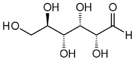
(a) Skeletal notation

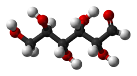
(b) 3D representation

Figure 1: D-glucose chain

Usually, a mathematical language is restricted to certain types of symbols such as numbers, letters or operators. To have an all-encompassing language, we have to extend our notion of what a symbol is. For us, we will allow the symbols to be graphs, diagrams, geometrical shapes and even 3D objects (represented in 2D or not). This allows us to have a language which has a two dimensional notation, an inline notation and a three dimensional version. Diagrammatics notation is already being successfully used in physics, mathematics and biology. In Physics, Feynmann diagrams [FeynmanA, FeynmanB] have proven to be a powerful tool and Penrose’s tensor diagrammatic notation is proposing a new way to do tensor calculus [Penrose]. In mathematics, diagrams are at the heart of graph theory and knot theory. As a notation, the language of commutative diagrams of category theory is now an essential tool in investigating highly abstract mathematical structures [MacLane] and different diagrammatic notations have been used to further study category theory [Selinger]. In Biology, textbooks use many types of diagrams to help the reader to understand. While these diagrams are not standardized, it could be fruitful to have a standard notation to enhance access to knowledge. With all the new capabilities of text editing and access 3D software, we are in a position to transition out of line-by-line mathematical notation and explore diagrams and 3D notations.

In this paper, to help understand, we will often use the two dimensional visual language and make extensive use of colors to simplify the notation. Colors can be always be replaced by numbered subscript or superscript, but its use helps to make the notation lighter. The visual notation is good for communication and understanding, but the inline notation is very important since it is the basis of computation. It will quickly become clear that the inline version of a structure can be cumbersome, since even colors need to be replaced by a subscript or superscript notation. We will introduce the visual notation in parallel with the basic inline notation. In the construction of mathematical models, we will not restrict ourselves to a particular one, but will switch between them in a way which is beneficial for understanding.

4.2 Basic Notation

4.2.1 Forms

In our language, any collection of symbols will be called a form. There are no restrictions on what a form can be. They can be letters, numbers, mathematical symbols, graphs, planar figures, 3D geometric shapes, people and collections of objects. We will only have to be careful when handling the special characters ‘$\rhd$’ and ‘$=$’. This language could be seen as a calculus of forms where forms can be anything we decide to name or distinguish.

4.2.2 Transformations

As time passes, things or the forms we see are always changing. A seed becomes a sprout and the sprout becomes a tree. In our attempt to understand the world, we make observations such as “this type of seed will give a certain type of tree with many different characteristics such as the shape of the leaves and cellular structure”. In the case of the seed-tree observations, we usually think of the seed as being the cause of the tree and not the other way around. As presented above, we will denote this are $\framebox{$Tree\rhd Seed$}$ and call such a structure a transformation. Transformations are forms having potential to change other forms. The transformation $\framebox{$Tree\rhd Seed$}$ can be understood as representing the process where a Seed is replaced by a Tree, a seed transforming into a tree or a seed becoming a tree. The right-hand side of the symbol $\rhd$ will be called the cause of the transformation and the left-hand side will be called the effect of the transformation. It should be visualized as the potential for the word $Tree$ to slide down the directed triangle and replace the word $Seed$.

To observe the process of the becoming of a tree from a seed; there needs to be a seed present. This can be represented as $\framebox{$Tree\rhd Seed$}\rightarrow(Seed)$ and will be called a system. The Seed at the right end of the arrow and between the parentheses ‘$(\,)$’ indicates the presence of the Seed. This ordered set that is acted on by some transformations will be called the initial form of the of these transformations. In the present case, we say that $(Seed)$ is the initial form of the transformation $\framebox{$Tree\rhd Seed$}$. The structure $\framebox{$Tree\rhd Seed$}$ can be seen as the potential of transformation of a seed into a tree and will only transform a seed in a tree when a seed is present. Eventually, we will have many elements in the initial form and unless said otherwise, we will consider that order in which the element appears as important. For example, $(A,B)$ is not considered to be the same as $(B,A)$.

We can represent the system $\framebox{$Tree\rhd Seed$}\rightarrow(Seed)$ in a diagram form as follows.

(1)

Or it can be represented as the following diagram, since it is understood that the side to where the triangle is pointing is the form that will be replaced.

(2)

In the diagram notation, the initial form will be denoted by a shape drawn with dash lines. We will use mostly shapes such as dashed circles, ellipses and rectangles.

4.2.3 Reduction

The act of applying the transformation $\framebox{$Tree\rhd Seed$}$ to the form $(Seed)$ is said to be a reduction of the system $\framebox{$Tree\rhd Seed$}\rightarrow(Seed)$ to the form $(Tree)$. This reduction is indicated by a double arrow ‘$\Rightarrow$’ and is written as

$$\framebox{$Tree\rhd Seed$}\rightarrow(Seed)\Rightarrow(Tree).$$

This expression is read as the transformation $\framebox{$Tree\rhd Seed$}$ applied to the form $(Seed)$ and reduces to the form $(Tree)$. It is important to note that the transformation is applied only once and then disappears after the reduction. When multiple transformations are used in a system, a reduction can refer to the final form where all transformations have been applied or all the steps leading to that final form are complete.

Seeds come in many types, so we can extend our language further and apply the transformation such as $\framebox{$Pine\rhd Seed$}$ to multiple seeds. There are two interesting ways to do this. The first is by successively applying certain transformations to an ordered set containing multiple seeds. The second is by applying one transformation at a time without any definite order. The first is said to be applied in series and the second in parallel.

The number of transformations which can be applied on an initial form can be finite or infinite. In the theory of term rewriting systems, a main focus is to have systems which terminate after a finite number of reductions. For us, since we are mainly concerned about creating mathematical models, we are interested in all the steps of the reductions and this whether it terminates or not. An interesting question for us to ask is if a system has a period or a cycle. In biology, an example of periodic system is the cell cycle.

4.2.4 Series of transformations

A series of three transformation applied to an ordered set of three seeds is written as

$$\framebox{$Maple\rhd Seed$}\rightarrow\framebox{$Oak\rhd Seed$}\rightarrow\framebox{$Pine\rhd Seed$}\rightarrow(Seed,Seed,Seed)$$

The reduction sequence of this system is be done in three steps and is denoted as follows. The transformation closest to the initial form is applied first followed by the second closest and so on.

$$\begin{array}[]{c}\framebox{$Maple\rhd Seed$}\rightarrow\framebox{$Oak\rhd Seed$}\rightarrow\framebox{$Pine\rhd Seed$}\rightarrow(Seed,Seed,Seed)\\ \Downarrow\\ \framebox{$Maple\rhd Seed$}\rightarrow\framebox{$Oak\rhd Seed$}\rightarrow(Seed,Pine,Seed)\\ \Downarrow\\ \framebox{$Maple\rhd Seed$}\rightarrow(Oak,Pine,Seed)\\ \Downarrow\\ (Oak,Pine,Maple)\\ \end{array}$$

Since all the elements of the initial form are the same, the transformation $\framebox{$Pine\rhd Seed$}$ can replace any choice of Seed. If one wants to differentiate between the Seeds, we could rename them as in the following example.

$$\framebox{$Maple\rhd Seed3$}\rightarrow\framebox{$Oak\rhd Seed2$}\rightarrow\framebox{$Pine\rhd Seed1$}\rightarrow(Seed3,Seed1,Seed2)$$

We now introduce superscript to the transformations. If we have a series of the same transformation being applied on an initial form, we will write this in a more compact notation by writing as a superscript an integer followed by the letter ‘$S$’ which indicates that the transformation is applied in series. For example,

$$\framebox{$Tree\rhd Seed$}\rightarrow\framebox{$Tree\rhd Seed$}\rightarrow\framebox{$Tree\rhd Seed$}\rightarrow(Seed,Seed,Seed)$$

can be written as

$$\framebox{$Tree\rhd Seed$}^{\,3S}\rightarrow(Seed,Seed,Seed).$$

Another example with two different types of transformation is to write

$$\framebox{$Oak\rhd Seed$}^{\,7S}\rightarrow\framebox{$Pine\rhd Seed$}^{\,10S}\rightarrow(Seed,Seed,Seed,Seed,Seed)$$

to represent 10 successive applications of the transformation $\framebox{$Pine\rhd Seed$}$ followed by a series of 7 applications of $\framebox{$Oak\rhd Seed$}$.

It is important to note that when no superscript is written, it is assumed to mean a superscript of $1S$. For example, $\framebox{$Tree\rhd Seed$}^{\,1S}$ is equivalent to $\framebox{$Tree\rhd Seed$}$.

We can also use the infinity symbol ‘$\infty$’ to denote that the transformation is continuously applied when needed. Thus the system

$$\framebox{$Oak\rhd Seed$}^{\,\infty S}\rightarrow(Seed,Seed,Seed,Seed,Seed),$$

reduces to

$$\framebox{$Oak\rhd Seed$}^{\,\infty S}\rightarrow(Oak,Oak,Oak,Oak,Oak).$$

If we want to replace all that can be replaced, we use the sharp symbol ‘$\sharp$’ to denote that the transformation is applied until it reaches a step where it cannot replace another element of the initial form, then the transformation disappears. In other words, it replaces all it can and then disappears. For example, the system

$$\framebox{$Oak\rhd Seed$}^{\,\sharp S}\rightarrow(Seed,Seed,Seed,Seed,Seed),$$

reduces to

$$(Oak,Oak,Oak,Oak,Oak).$$

4.2.5 Parallel transformations

When transformations are applied in parallel, we will denote this by grouping them in box brackets ‘$[\,]$’. For example, two transformations applied on an initial form containing three seeds is written as

$$[\,\framebox{$Pine\rhd Seed$},\framebox{$Oak\rhd Seed$}\,]\rightarrow(Seed).$$

When parallel transformations are applied to an ordered set, any transformation that can be applied can be chosen to be applied first. After it has been applied, it disappears and another one is chosen. An example of reduction is

$$[\,\framebox{$Pine\rhd Seed$},\framebox{$Oak\rhd Seed$}\,]\rightarrow(Seed)$$

$$\Downarrow$$

$$[\,\framebox{$Oak\rhd Seed$}\,]\rightarrow(Pine)$$

But since the transformations were in parallel, we could also have

$$[\,\framebox{$Pine\rhd Seed$},\framebox{$Oak\rhd Seed$}\,]\rightarrow(Seed)$$

$$\Downarrow$$

$$[\,\framebox{$Pine\rhd Seed$}\,]\rightarrow(Oak)$$

We now introduce the diagram notation. The system

$$[\,\framebox{$Pine\rhd Seed$},\framebox{$Oak\rhd Seed$},\framebox{$Maple\rhd Seed$}\,]\rightarrow(Seed,Seed,Seed),$$

which contains three parallel transformations can also be represented as the following diagram.

(3)

It is also possible to reduce the number of arrows in the diagram by grouping the transformation under a bracket ‘$]$’ as seen below.

(4)

Similarly to series of transformations, there is a superscript notation if the same transformation is applied multiple times on an initial form. This is done by writing as a superscript an integer followed by the letter ‘$P$’ which indicates that the transformation is applied in parallel. For example,

$$[\,\framebox{$Tree\rhd Seed$},\framebox{$Tree\rhd Seed$},\framebox{$Tree\rhd Seed$}\,]\rightarrow(Seed,Seed,Seed)$$

can be written as

$$[\,\framebox{$Tree\rhd Seed$}^{\,3P}\,]\rightarrow(Seed,Seed,Seed).$$

Another example with two different types of transformations, is to write

$$[\,\framebox{$Oak\rhd Seed$}^{\,2P},\framebox{$Pine\rhd Seed$}^{\,3P}\,]\rightarrow(Seed,Seed,Seed,Seed,Seed)$$

to represent the following diagram.

(5)

In a similar way to series of transformations, we can also use the infinity symbol ‘$\infty$’ to denote that a transformation is continuously applied and the sharp symbol ‘$\sharp$’ to indicate that the transformation replaces all it can from the initial form and then disappears.

4.2.6 Arising and Dissolution

This language permits creation of new objects in an ordered set by using a transformation in which the right or left hand-side of the transformation is empty. An example is given by the following transformation of making rabbits appear in a grass and flower field. This is an interesting property, since this gives us a mathematical way to add new objects to a set of forms.

$$\begin{array}[]{c}\framebox{$rabbit\,\,\rhd\hskip 28.45274pt$}^{\,3S}\rightarrow(grass,flowers)\\ \Downarrow\\ \framebox{$rabbit\,\,\rhd\hskip 28.45274pt$}^{\,2S}(grass,flowers,rabbit)\\ \Downarrow\\ \framebox{$rabbit\,\,\rhd\hskip 28.45274pt$}(grass,rabbit,flowers,rabbit)\\ \Downarrow\\ (grass,rabbit,flowers,rabbit,rabbit)\end{array}$$

Similarly, as seen in the following example we can dissolve a form.

$$\begin{array}[]{c}\framebox{$\hskip 28.45274pt\rhd\,\,cup$}^{\,2S}\rightarrow(cup,spoon,cup)\\ \Downarrow\\ \framebox{$\hskip 28.45274pt\rhd\,\,cup$}\rightarrow(cup,spoon)\\ \Downarrow\\ (spoon)\end{array}$$

4.2.7 Position Pairing in Transformations

Until now in our transformations, there was only one term on each side of the directed triangle. We now allow multiple terms on each side of the triangle. Let’s revisit our seed example.

A seed turns into a tree if there is a soil, water and sun. After the appearance of the tree the soil is still there and the sun is still present. We could view the sun and the soil to be the supporting conditions. After a transformation is applied, the supporting conditions will stay there and will not change. In practice, we can say that a very small amount of soil and energy from the sun was used, but in our present model, we will consider that it is a negligible amount. To do this we will identify together elements on each side of the triangle. This is done by respecting the position of the terms on both sides of the directed triangle. To indicate that a form $A$ in a certain position has been replace by another form $B$, we write the $A$ and $B$ at the same position on each side of the directed triangle. If a form is unaffected by the transformation, the form will appear at the same place on both sides. Another way to view this is to think that $B$ has been paired with $A$. This is similar to functions where each element of the domain is paired with an element of the range of the function.

Here is an example of our seed turning into a tree with the conditions of sun and soil.

(6)

This will reduce to

(7)

Notice that the terms of initial form are not in the same configuration as seen in the transformation. The position is only important in the transformation and is meant to indicate which forms are paired together. When a transformation is applied on the initial form, the elements are replaced at the place they are found in the initial form as seen above.

We now look at another example where a seed and water becomes a tree based on the conditions of the sun and soil. Notice that the water disappeared and that the seed was replaced by a tree. Note that this system makes an implicit use of the dissolution transformations when the water is removed.

(8)

In the next example, the water disappeared, the seed was replaced by a tree and an apple appears in some position.

(9)

The next example shows that the replacing object can be positioned at another position than the replaced object. Here the triangle contracts to a point in the center of the triangle.

$$[linewidth=0.04,dimen=outer](4.02,2.99)(1.0,0.92)[linewidth=0.04,dimen=outer](12.85,2.65)(1.7,1.44)[linewidth=0.04,dimen=outer](6.17,2.65)[linewidth=0.04,dimen=outer](4.02,2.99)(1.0,0.92)[linewidth=0.04,dimen=outer](12.85,2.65)(1.7,1.44)[linewidth=0.04,dimen=outer](6.17,2.65)$$ (10)