RESONANT THRESHOLD TWO-PHOTON $e^{-}e^{+}$
PAIR PRODUCTION ONTO THE LOWEST LANDAU
LEVELS IN A STRONG MAGNETIC FIELD

Abstract

The process of electron-positron pair production by two photons in a strong magnetic field has been studied.  The process kinematics is considered, and the probability amplitude for arbitrary polarizations of particles is found.  The resonance conditions are established, and the resonant cross-section is estimated in the case where the electron and the positron occupy the lowest levels ($l_{e}=$ 1, $l_{p}=$ 0) that satisfy these resonance conditions.

1 Introduction

The researches of quantum electrodynamic (QED) processes that take place at the collisions of heavy ions have a challenging character, which is associated with the progress achieved in the domain of heavy-ion accelerators.  In such experiments, the main attention is usually concentrated on the researches dealing with properties of the strong interaction.  However, the QED processes can also be studied even if nuclei do not approach each other at the distance characteristic of the strong interaction [1,​ 2].

In the course of collisions between heavy ions, the extremely intensive, rapidly varying electromagnetic fields are generated.  The resulting strength of the field can exceed the critical QED value $H_{c}=\frac{m^{2}c^{3}}{e\hbar}\approx$ $\approx 4.41\times 10^{13}$ Gs, which, according to the theoretical reasoning, is the vacuum excitation threshold [3].  This fact opens vast opportunities for testing the QED predictions in the range of strong fields.  A wide program of such experiments is planned to be fulfilled on the future FAIR (Facility for Antiproton and Ion Research) installation, which is under construction on the basis of the GSI (GSI Helmholtz Centre for Heavy Ion Research, Darmstadt, Germany) [4].

The production of electron-positron pairs at the collisions between ions is a challenging problem from the theoretical and experimental viewpoints.  In particular, the production of a pair with the electron in a bound state changes the charge of one of the ions and is one of the principal origins of beam losses in modern colliders. On the other hand, the pair production by a strong total supercritical field of heavy nuclei is the evidence of a bound state diving in the negative energy continuum, as well as of the transition of the vacuum into a new state [3].

A poorly studied issue in the problem of $e^{-}e^{+}$ pair production at the collision of moving ions is the influence of the magnetic field created by the ions.  Simple estimates testify that the field between the ions can reach the critical value $H_{c}$ or can even exceed it already at collision energies of the Coulomb barrier order.  However, in the majority of researches, only the Coulomb field of ions is taken into account.  The attempts to reveal the influence of a magnetic field were made for the first time in works [5,​ 6,​ 7] in the framework of the model of quasimolecule (for low-energy collisions).  The corresponding numerical calculations showed the absence of the effect; however, the interaction of the created pair with the magnetic field was not taken into consideration.

In work [8], the assumption that the created electron-positron pair captures the magnetic field similarly to the phenomenon, where the magnetic field lines “are frozen” into a plasma, was substantiated.  The corresponding estimates testify that the lifetime of the self-consistent system “pair + magnetic field” considerably exceeds the nuclear transit time.  Therefore, the magnetic field can substantially affect the process.  The presence of characteristic resonances in the corresponding channels can be the observable evidence of QED processes in the magnetic field created by colliding ions.

It has to be noted that, in the EPOS and ORANGE experiments carried out at the GSI, anomalous peaks were revealed in the channel of electron-positron pair production [9,​ 10,​ 11].  The nature of peaks was not elucidated, and their very existence was not confirmed.  In view of the similarity between the spectrum of anomalous peaks and the quasiequidistant spectrum of electron energy levels in the magnetic field, it is quite probable that further researches of the role of a magnetic field in ionic collisions will deepen our understanding of this phenomenon.

According to the results of work [8], the lifetime of the magnetic field substantially exceeds the characteristic time of electromagnetic interaction.  Therefore, the process can be considered as the electron-positron pair production in a constant uniform magnetic field.  This approximation allows one to reveal the main features of the process and, at the same time, to obtain simple analytical expressions for the cross-section.  Moreover, if the energy of ions is sufficiently high, the conditions for the application of the equivalent-photon method [12] are satisfied.  Hence, in the simplest case, our problem is approximately reduced to the study of the process of two-photon electron-positron pair production in a magnetic field.

Let us also mention possible applications of the results of this work to the problem of electron cooling of heavy-ion beams.  The essence of the method consists in a decrease of the effective beam temperature owing to the collision of ions in the beam with electrons that move together with the beam and possess a small spread of velocities [13,​ 14,​ 15]. Although the method of electron cooling has been known for a long time and is widely used in accelerating facilities, the experimentally observed difference between the cooling efficiency for positive and negative particles remains unexplained [16].  In particular, the electron cooling of an antiproton beam is planned to be used in the HESR accumulator (FAIR), and this fact substantiates the problem urgency [17,​ 18].

The application of the method of quantum field theory to the problem of electron cooling [19,​ 20] has considerable advantages in comparison with others (the method of pair collisions, the dielectric model, and so forth), because it contains no phenomenological parameters.  The corresponding stopping power is expressed in terms of the polarization operator.  The difference between the cooling of protons and antiprotons may probably be described in the second Born approximation.  However, according to the optical theorem, the imaginary part of the polarization operator in the second order is equal to the total probability of the process of two-photon pair production.

For the first time, the process of two-photon electron-positron pair production in a magnetic field was considered in work [21] in the simplest case of the head-on photon collision along the magnetic field.  In work [22], this process was analyzed for an arbitrary direction of photon propagation, but under the assumption that the energy of each photon is insufficient for the pair production in the one-photon process.  This condition excludes the possibility of the resonance character of the reaction.

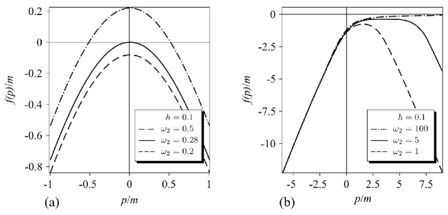
Fig. 1.: Function $f(p_{ez})/m$ plotted for the numbers of Landau levels $l_{e}=2$ and $l_{p}=1$.  The frequency of the first photon in terms of the electron mass units, $\omega_{1}=2$. $\theta_{1,2}=\pi/2$ (a) and 0 (b)

In this work, in contrast to the earlier researches, the process was considered in the case where the energy of one of the photons or each of them is sufficient for the pair production.  The total amplitude of the process with arbitrary polarizations of particles and the conditions for the resonant character of the process are determined.  The process cross-section is estimated for the lowest Landau levels that satisfy the resonance conditions.

Throughout the work, the relativistic system of units, $\hbar=c=1$, is used.

2 Kinematics

It is known [12] that the electron occupies discrete energy levels in a uniform magnetic field,

$$E=\sqrt{p_{z}^{2}+\tilde{m}^{2}},\quad\tilde{m}=m\sqrt{1+2lh},$$ (1)

where $p_{z}$ is the longitudinal momentum component with respect to the field, $l$ the level number, and $h$ the magnetic field measured in the units of $H_{c}$.  In the magnetic field, the conservation laws of the energy and the momentum component parallel to the field are obeyed and have the following form for the process of two-photon electron-positron pair production:

$$\begin{array}[]{l}\displaystyle E_{e}+E_{p}=W,\\[2.84526pt] \displaystyle p_{ez}+p_{pz}=K.\end{array}$$ (2)

Here, $W=\omega_{1}+\omega_{2}$ is the total energy, and $K=k_{1z}\,+$ $+\,k_{2z}$ is the total longitudinal momentum of photons.

Let us determine the threshold conditions of the pair production onto some Landau levels $l_{e}$ and $l_{p}$.  First, let us introduce the auxiliary function $f(p_{ez})=\omega_{1}+\omega_{2}-E_{e}-E_{p}$.  The process threshold is determined by the condition $f(p_{m})=0$, where $p_{m}$ is the point of a maximum of the function.  After the differentiation, we find the value of electron momentum at the maximum,

$$p_{m}=\frac{\tilde{m}_{e}K}{\tilde{m}_{e}+\tilde{m}_{p}}.$$ (3)

In view of the previous relations, the threshold values of the energy and the electron and positron momenta are expressed as follows:

$$E_{e}^{\prime}=\frac{\tilde{m}_{e}}{\tilde{m}_{e}+\tilde{m}_{p}}W^{\prime},\quad p_{ez}^{\prime}=\frac{K^{\prime}E_{e}^{\prime}}{W^{\prime}},$$ (4)

$$E_{p}^{\prime}=\frac{\tilde{m}_{p}}{\tilde{m}_{e}+\tilde{m}_{p}}W^{\prime},\quad p_{pz}^{\prime}=\frac{K^{\prime}E_{p}^{\prime}}{W^{\prime}}.$$ (5)

From whence, the condition for the reaction threshold takes the form

$$W^{\prime 2}-K^{\prime 2}=(\tilde{m}_{e}+\tilde{m}_{p})^{2}.$$ (6)

In the general case (above the threshold), system (2) gives the following expression for the momenta of particles:

$$p_{ez}=\frac{aK\pm bW}{2M^{2}}.$$ (7)

Here, the notations

$$a=M^{2}-\tilde{m}_{p}^{2}+\tilde{m}_{e}^{2}\!,$$ (8)

$$b^{2}=M^{4}-2M^{2}((\tilde{m}_{e})^{2}+(\tilde{m}_{p})^{2})+4(l_{p}-l_{e})^{2}h^{2}\!,$$ (9)

$$M^{2}=W^{2}-K^{2}$$ (10)

were introduced.  The process is evidently impossible, if both photons move in parallel to ${\bf H}$, because $K^{2}=W^{2}$ in this case, and condition (6) is not satisfied.  This situation is illustrated in Fig. 1.

Note that the Lorentz transformations along ${\bf H}$ do not change the magnetic field itself.  Therefore, without any loss of generality, the reference frame can be chosen to exclude the longitudinal momentum of photons: $K=0$.  In this reference frame, $p_{ez}=-p_{pz}$, and the threshold conditions have a simpler form,

$$W^{\prime}=\tilde{m}_{e}+\tilde{m}_{p},\quad p_{ez}^{\prime}=p_{pz}^{\prime}=0.$$ (11)

3 Amplitude

The electron and positron wave functions look like[23]

$$\begin{array}[]{l}\displaystyle\Psi_{e}=\frac{1}{\sqrt{S}}e^{-i(Et-p_{y}y-p_{z}z)}\psi_{e}(\zeta^{-}),\\[11.38109pt] \displaystyle\Psi_{p}=\frac{1}{\sqrt{S}}e^{+i(Et-p_{y}y-p_{z}z)}\psi_{p}(\zeta^{+}),\end{array}$$ (12)

where $\zeta^{\pm}=m\sqrt{h}(x\mp p_{y}/m^{2}h)$,

$$\psi_{e}(\zeta^{-})=C_{e}\biggl{[}i\sqrt{\tilde{m}_{e}-\mu_{e}m}U_{l}(\zeta^{-})\,+$$

$$+\,\mu_{e}\sqrt{\tilde{m}_{e}+\mu_{e}m}U_{l-1}(\zeta^{-})\gamma^{1}\biggr{]}u_{e},$$ (13)

$$\psi_{p}(\zeta^{+})=C_{p}\Bigl{[}i\sqrt{\tilde{m}_{p}+\mu_{p}m}U_{l}(\zeta^{+})\,-$$

$$-\,\mu_{p}\sqrt{\tilde{m}_{p}-\mu_{p}m}U_{l-1}(\zeta^{+})\gamma^{1}\Bigr{]}u_{p}.$$ (14)

Here, $S$ is the normalization area, $U_{l}(x)$ the Hermite function, $\mu_{e,p}$ are the doubled spin projections of the electron and the positron, $C_{e,p}$ the normalization constants, and $u_{e,p}$ the constant bispinors:

$$C_{e,p}=\frac{1}{2}\sqrt{\frac{\sqrt{eH}}{E_{e,p}\tilde{m}_{e,p}}}\!,$$ (15)

$$u_{e,p}=\frac{1}{R_{e,p}}\left(0,\>\pm R^{2}_{e,p},\>0,\>p_{{(e,p)}z}\right)\!,$$ (16)

$$R_{e,p}=\sqrt{E_{e,p}-\mu_{e,p}\tilde{m}_{e,p}},$$ (17)

where the sign “$-$” in $u_{e,p}$ corresponds to the electron.  The wave functions (12)–(14) correspond to the $(0;0,xH,0)$ gauge of the electromagnetic 4-potential.

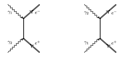
Fig. 2.: Feynman diagrams for the two-photon $e^{-}e^{+}$ pair production in a magnetic field

For the wave function of the initial photon, the standard expression is used [12],

$$A^{\nu}=\sqrt{\frac{2\pi}{\omega V}}e^{\nu}e^{ikx}\!,$$ (18)

where $V$ is the normalization volume, $e^{\nu}=(0,{\bf e})$ is the 4-vector of photon polarization, and

$$\mathrm{e}=\left(\!\!\begin{array}[]{c}\cos\phi\cos\theta\cos\alpha-e^{i\beta}\sin\phi\sin\alpha\\ \sin\phi\cos\theta\cos\alpha+e^{i\beta}\cos\phi\sin\alpha\\ -\sin\theta\cos\alpha\end{array}\!\!\right)\!\!.$$ (19)

Here, $\phi$ and $\theta$ are the azimuthal and polar angles, respectively; and $\alpha$ and $\beta$ are polarization parameters.

Green’s function of a virtual electron looks like [24]

$$G(x-x^{\prime})=\frac{-m\sqrt{h}}{(2\pi)^{3}}\int d^{3}ge^{-i\Phi}\sum\limits_{n}\frac{G_{H}(x,x^{\prime})}{g_{0}^{2}-E_{n}^{2}},$$ (20)

$$G_{H}(x,x^{\prime})=U_{n}U_{n}^{\prime}(\gamma P+m)\tau\,+$$

$$+\,im\sqrt{2nh}U_{n-1}U^{\prime}_{n}\gamma^{1}\tau-im\sqrt{2nh}U_{n}U_{n-1}^{\prime}\tau\gamma^{1}\,+$$

$$+\,U_{n-1}U^{\prime}_{n-1}(\gamma P+m)\tau^{*},$$ (21)

where $\gamma$’s are Dirac gamma matrices,

$$\Phi=g_{0}(t-t^{\prime})-g_{y}(y-y^{\prime})-g_{z}(z-z^{\prime}),$$ (22)

$$\tau=\frac{1}{2}(1+i\gamma_{2}\gamma_{1}),$$ (23)

$$P=(E_{n},0,0,g_{z}).$$ (24)

The argument of Hermite functions in Eq. (21) looks like

$$\rho(x)=m\sqrt{h}x+g_{y}/m\sqrt{h},$$

and the primed function means its dependence on $\rho(x^{\prime})$.

According to the QED rules, the two-photon electron-positron pair production amplitude is determined as

$$S_{fi}=-ie^{2}\int d^{4}xd^{4}x^{\prime}\Bigl{[}\bar{\Psi}_{e}(A_{1}\gamma)G(x-x^{\prime})(A^{\prime}_{2}\gamma)\Psi_{p}^{\prime}\,+$$

$$+\,\bar{\Psi}_{e}(A_{2}\gamma)G(x-x^{\prime})(A^{\prime}_{1}\gamma)\Psi_{p}^{\prime}\Bigr{]},$$ (25)

where the primed quantities depend on $x^{\prime}$.  Figure 2 demonstrates the Feynman diagrams that correspond to amplitude (25).  Substituting the wave functions and the propagator into Eq. (25) and carrying out the corresponding transformations, we obtain the amplitude in the form

$$S_{fi}^{(1)}=\frac{-ie^{2}(2\pi)^{4}}{4VS\sqrt{\omega_{1}\omega_{2}\tilde{m}_{e}\tilde{m}_{p}E_{e}E_{p}}}\sum\limits_{n=0}^{\infty}\frac{\sum_{j=1}^{16}B_{j}}{g_{0}^{2}-E_{n}^{2}}\,\times$$

$$\times\,\delta^{3}(\gamma_{1}+\gamma_{2}-e^{-}-e^{+}),$$ (26)

where the terms $B_{j}$ look like

$$B_{1}=-i\mu_{e}M_{e+}^{p+}e_{1}T_{2}^{-}\,\times$$

$$\times\,(mS^{+}\!+\!E_{n}S^{-}\!\!-\!g_{z}A^{-})I^{(1)}_{l_{e}-1,n-1}I^{(2)}_{n-1,l_{p}},$$

$$B_{2}=\mu_{e}\mu_{p}M_{e+}^{p-}e_{1}e_{2}\,\times$$

$$\times\,(mA^{-}\!+E_{n}A^{+}\!+g_{z}S^{+})I^{(1)}_{l_{e}-1,n-1}I^{(2)}_{n-1,l_{p}-1},$$

$$B_{3}=i\mu_{e}M_{e+}^{p+}e_{2}T_{1}^{-}(mS^{+}\!\!+E_{n}S^{-}\!\!+\!g_{z}A^{-})I^{(1)}_{l_{e}-1,n}I^{(2)}_{n,l_{p}},$$

$$B_{4}=\mu_{e}\mu_{p}M_{e+}^{p-}T_{1}^{-}T_{2}^{+}\,\times$$

$$\times\,(mA^{-}\!+E_{n}A^{+}\!-g_{z}S^{+})I^{(1)}_{l_{e}-1,n}I^{(2)}_{n,l_{p}-1},$$

$$B_{5}=-\mu_{e}M_{e+}^{p+}m\sqrt{2nh}\>e_{1}e_{2}A^{-}I^{(1)}_{l_{e}-1,n-1}I^{(2)}_{n,l_{p}},$$

$$B_{6}=-i\mu_{e}\mu_{p}M_{e+}^{p-}m\sqrt{2nh}\>e_{1}T_{2}^{+}S^{+}I^{(1)}_{l_{e}-1,n-1}I^{(2)}_{n,l_{p}-1},$$

$$B_{7}=-\mu_{e}M_{e+}^{p+}m\sqrt{2nh}\>T_{1}^{-}T_{2}^{-}A^{-}I^{(1)}_{l_{e}-1,n}I^{(2)}_{n-1,l_{p}},$$

$$B_{8}=-i\mu_{e}\mu_{p}M_{e+}^{p-}m\sqrt{2nh}\>e_{2}T_{1}^{-}S^{+}I^{(1)}_{l_{e}-1,n}I^{(2)}_{n-1,l_{p}-1},$$

$$B_{9}=M_{e-}^{p+}T_{1}^{-}T_{2}^{+}\,\times$$

$$\times\,(mA^{-}\!\!-E_{n}A^{+}\!\!+g_{z}S^{+})I^{(1)}_{l_{e},n-1}I^{(2)}_{n-1,l_{p}},$$

$$B_{10}=-i\mu_{p}M_{e-}^{p-}e_{2}T_{1}^{+}\,\times$$

$$\times\,(mS^{+}\!\!-E_{n}S^{-}\!\!-g_{z}A^{-})I^{(1)}_{l_{e},n-1}I^{(2)}_{n-1,l_{p}-1},$$

$$B_{11}=M_{e-}^{p+}e_{1}e_{2}(mA^{-}\!\!-E_{n}A^{+}\!\!-g_{z}S^{+})I^{(1)}_{l_{e},n}I^{(2)}_{n,l_{p}},$$

$$B_{12}=i\mu_{p}M_{e-}^{p-}e_{1}T_{2}^{+}\,\times$$

$$\times\,(mS^{+}\!\!-E_{n}S^{-}\!\!+g_{z}A^{-})I^{(1)}_{l_{e},n}I^{(2)}_{n,l_{p}-1},$$

$$B_{13}=-iM_{e-}^{p+}m\sqrt{2nh}\>e_{2}T_{1}^{+}S^{+}I^{(1)}_{l_{e},n-1}I^{(2)}_{n,l_{p}},$$

$$B_{14}=\mu_{p}M_{e-}^{p-}m\sqrt{2nh}\>T_{1}^{+}T_{2}^{+}A^{-}I^{(1)}_{l_{e},n-1}I^{(2)}_{n,l_{p}-1},$$

$$B_{15}=-iM_{e-}^{p+}m\sqrt{2nh}\>e_{1}T_{2}^{-}S^{+}I^{(1)}_{l_{e},n}I^{(2)}_{n-1,l_{p}},$$

$$B_{16}=\mu_{p}M_{e-}^{p-}m\sqrt{2nh}\>e_{1}e_{2}A^{-}I^{(1)}_{l_{e},n}I^{(2)}_{n-1,l_{p}-1}.$$

Here, $e_{1,2}$ are the $z$-components of the photon polarization vectors, and the following notations are introduced:

$$M_{e\pm}^{p\pm}=\sqrt{\tilde{m}_{e}\pm\mu_{e}m}\sqrt{\tilde{m}_{p}\pm\mu_{p}m},$$ (27)

$$T_{j}^{\pm}=e_{jx}\pm ie_{jy},\quad j=1,2,$$ (28)

$$A^{\pm}=\frac{R_{e}^{2}R_{p}^{2}\pm p_{ez}p_{pz}}{R_{e}R_{p}},$$ (29)

$$S^{\pm}=\frac{R_{e}^{2}p_{pz}\pm R_{p}^{2}p_{ez}}{R_{e}R_{p}},$$ (30)

where $R_{e,p}$ are determined by Eq. (17).  The functions $I_{l,l^{\prime}}^{(j)}$ are typical of QED problems with the magnetic field [28,​ 29]:

$$I_{l,l^{\prime}}^{(j)}=e^{-\Phi_{j}}\frac{(i\sqrt{\eta_{j}})^{\Lambda-\lambda}}{(\Lambda-\lambda)!}\sqrt{\frac{\Lambda!}{\lambda!}}F(-\lambda,\Lambda-\lambda+1,\eta_{j}),$$ (31)

$$\Lambda=\max(l,l^{\prime}),\quad\lambda=\min(l,l^{\prime}),$$ (32)

$$\Phi_{j}=\frac{\eta_{j}}{2}+\frac{k_{jx}\kappa_{j}}{2m^{2}h}+i\phi_{j}(l-l^{\prime}),$$ (33)

$$\kappa_{1}=2p_{ey}-k_{1y},$$ (34)

$$\kappa_{2}=k_{2y}-2p_{py},$$ (35)

$$\eta_{j}=\frac{k_{jx}^{2}+k_{jy}^{2}}{2m^{2}h},$$ (36)

where $\phi_{j}$ are the azimuthal angles of photons, and $F(a,b,\eta)$ is the degenerate hypergeometric function.  The term that corresponds to the exchange diagram is obtained by swapping the subscripts: $1\rightleftarrows 2$.

4 Resonance Conditions

The process acquires a resonant character if its kinematics permits an on-shell virtual electron state, i.e.  if the quantities $g_{0}$ and $g_{z}$ satisfy the standard relation between the electron energy and the momentum in a magnetic field,

$$g_{0}^{2}=g_{z}^{2}+m^{2}+2nhm^{2}=E_{n}^{2}.$$ (37)

In this case, the denominator in propagator (20) vanishes. In order to avoid the resulting divergence, the radiation width of a virtual state, $\Gamma$, is introduced according to the Breit–Wigner prescription [25],

$$E_{n}\rightarrow E_{n}-\frac{i}{2}\Gamma.$$ (38)

Let us determine the resonance frequencies of photons in the ultra-quantum approximation corresponding to the conditions

$$l\sim 1,\quad lh\ll 1.$$ (39)

Note that those conditions are characteristic of subcritical fields.  We confine the consideration to the case where both photons propagate normally to the magnetic field, and their energy is close to the threshold one, i.e.

$$\begin{array}[]{l}\displaystyle k_{1z}=k_{2z}=0,\\[8.53581pt] \displaystyle W=\tilde{m}_{e}+\tilde{m}_{p}+\delta W,\quad\delta W\lesssim mh.\end{array}$$ (40)

Then, expression (7) for the momentum simplifies,

$$p_{ez}=\sqrt{m\delta W}.$$ (41)

Taking into account that the conservation laws are satisfied at the diagram vertices, we use condition (37) to find the resonance frequencies for the first diagram,

$$\begin{array}[]{l}\displaystyle\omega_{1}=mh(l_{e}-n),\\[8.53581pt] \displaystyle\omega_{2}=2m+mh(l_{p}+n)+\delta W.\end{array}$$ (42)

From whence, it is evident that the pair is produced by the hard photon, whereas the soft one stimulates the transition of a virtual electron between the Landau levels.  This result is not unexpected, because the process at the resonance can be regarded as the sequence of a one-photon pair production and a photon absorption.

5 Resonant Cross-Section

Let us estimate the resonant cross-section of the two-photon pair production in the ultra-quantum approximation.  Conditions (40)–(42) are supposed to be satisfied.  In addition, let us select the energetically favorable particle polarizations [26,​ 27] and the numbers of Landau levels that correspond to the lowest resonance:

$$\mu_{e}=-1,\quad\mu_{p}=+1,$$ (43)

$$l_{e}=1,\quad l_{p}=n=0.$$ (44)

In the sum over $n$ in amplitude (26), we keep only the resonant term with $n=0$, in which the denominator tends to zero.  In this case, the second diagram does not give a substantial contribution to the process, because the resonance conditions for it are not obeyed.

Taking the aforesaid, as well as expressions for resonance frequencies (42) and conditions (43) and (44), into account, let us expand amplitude (26) in a series in the small parameter $h$.  In the zero-order approximation, we obtain

$$S_{fi}\approx e^{i\Phi}e^{2}(2\pi)^{4}\frac{e^{-\frac{1}{h}}\sin\alpha_{1}\cos\alpha_{2}}{SV(p_{0}^{2}-E_{n}^{2})}\,\times$$

$$\times\,\delta^{3}(\gamma_{1}+\gamma_{2}-e^{-}-e^{+}).$$ (45)

According to the known QED rules, the process cross-section is determined as the squared probability amplitude multiplied by the interval of final states and divided by the flux $j$, i.e.

$$d\sigma=\frac{|S_{fi}|^{2}}{jT}\frac{Sd^{2}p_{e}}{(2\pi)^{2}}\frac{Sd^{2}p_{p}}{(2\pi)^{2}},$$ (46)

$$j=(1-\cos\chi)/V,$$ (47)

where $d^{2}p_{e(p)}=dp_{e(p)y}dp_{e(p)z}$, $T$ is the time, and $\chi$ the angle between the photons.

The integration of Eq. (46) over $d^{2}p_{p}$ can be executed with the help of $\delta$-functions.  The process cross-section does not depend on $p_{ey}$.  Therefore, the integration over $dp_{ey}$ is reduced to the multiplication of the expression by $p_{ey}$.  Hence, there emerges a multiplier $Sp_{ey}/V$.  According to work [28], we can get rid of it by identifying the normalization length $L=V/S$ with the coordinate of the Larmor orbit center, $x_{0}=p_{ey}/m^{2}h$.  Hence,

$$\frac{Sp_{ey}}{V}=m^{2}h.$$ (48)

The remaining integral over $dp_{ez}$ can be found using the relation

$$\delta(\omega_{1}+\omega_{2}-E_{e}-E_{p})=\frac{m}{2p_{ez}}\sum\delta(p_{ez}\pm\sqrt{m\delta W}).$$ (49)

In addition, let us express the quantities $\alpha_{1}$ and $\alpha_{2}$ in terms of the more convenient Stokes parameters,

$$\begin{array}[]{l}\displaystyle\sin^{2}\alpha_{j}=\frac{1}{2}(1-\xi_{3}^{(j)}),\\[8.53581pt] \displaystyle\cos^{2}\alpha_{j}=\frac{1}{2}(1+\xi_{3}^{(j)}).\end{array}$$ (50)

The ultimate expression for the resonant cross-section looks like

$$\sigma=\alpha^{2}\frac{\pi he^{-\frac{2}{h}}}{8(1-\cos\chi)}\sqrt{\frac{m}{\delta W}}\frac{(1-\xi_{3}^{(1)})(1+\xi_{3}^{(2)})}{(g_{0}-E_{n})^{2}+\frac{\Gamma^{2}}{4}}\!,$$ (51)

where $\alpha$ is the fine structure constant.

6 Conclusions

Let us analyze the obtained expression (51) and demonstrate that the resonant cross-section can be factorized into the probabilities of the first-order processes.  In the ultra-quantum approximation, the probabilities of the one-photon $e^{-}e^{+}$ pair production and the magnetobremsstrahlung look like [27]

$$\frac{dW^{\rm rad}_{1,0}}{du}\bigg{|}_{u=0}=\alpha\frac{mh^{2}}{4}(1-\xi_{3}^{(1)}),$$ (52)

$$W^{pp}_{1,0}=\alpha\frac{mh}{4\sqrt{\delta W/m}}e^{-\frac{2}{h}}(1+\xi_{3}^{(2)})$$ (53)

(here, conditions (37), (43), and (44) were used). Hence, the process cross-section (51) can be written in the form of Breit–Wigner formula,

$$\sigma=\frac{2\pi}{m^{2}h^{2}(1-\cos\chi)}\frac{\frac{dW^{\rm rad}_{1,0}}{du}|_{u=0}W^{pp}_{1,0}}{(g_{0}-E_{n})^{2}+\frac{\Gamma^{2}}{4}}.$$ (54)

At last, let us evaluate cross-section (51) in the case of the head-on collision of photons ($\chi=\pi$).  As an example, we choose the following values of parameters:

$$\xi_{3}^{(1)}=-1,\quad\xi_{3}^{(2)}=1,$$ (55)

$$h=0.1,\quad\delta W=mh.$$ (56)

Then the radiation width and the cross-section approximately equal

$$\Gamma\approx 7\times 10^{17}\>\mathrm{s}^{-1}\!,$$ (57)

$$\sigma\approx 2\times 10^{-2}\>\mathrm{barn}.$$ (58)

М.М. Дяченко, О.П. Новак, Р.I. Холодов
ПОРОГОВЕ РЕЗОНАНСНЕ ДВОФОТОННЕ
НАРОДЖЕННЯ $e^{-}e^{+}$ ПАРИ В СИЛЬНОМУ
МАГНIТНОМУ ПОЛI НА НАЙНИЖЧI РIВНI ЛАНДАУ
Р е з ю м е
В роботi розглянуто процес народження електрон-позитронної пари двома фотонами в сильному магнiтному полi. Дослiджена кiнематика та знайдена загальна амплiтуда процесу з довiльною поляризацiєю частинок. Знайдено умови резонансного перебiгу реакцiї та проведено оцiнку перерiзу для випадку, коли електрон та позитрон займають найнижчi рiвнi ($l_{e}=$ 1, $l_{p}=$ 0), що задовольняють умови резонансу.

References

- [1] G. Baur, K. Hencken, D. Trautmann et al., Phys. Rep. 364, 359 (2002).
- [2] G. Baur, K. Hencken, and D. Trautmann, Phys. Rep. 453, 1 (2007).
- [3] W. Greiner, B. Müller, and J. Rafelski, Quantum Electrodynamics of Strong Fields (Springer, Berlin, 1985).
- [4] W. Henning, FAIR Conceptual Design Report (Gesellschaft für Schwerionenforschung, Darmstadt, 2001).
- [5] G. Soff, J. Reinhardt, and W. Greiner, Phys. Rev. A 23, 701 (1981).
- [6] K. Rumrich, W. Greiner, and G. Soff, Phys. Lett. A 125, 394 (1987).
- [7] G. Soff and J. Reinhardt, Phys. Lett. B 211, 179 (1988).
- [8] P.I. Fomin and R.I. Kholodov, Dopov. Nat. Akad. Nauk Ukr., No. 12, 91 (1998).
- [9] H. Backe, L. Handschug, F. Hessberger et al., Phys. Rev. Lett. 40, 1443 (1978).
- [10] W. Koenig, F. Bosch, P. Kienle et al., Z. Phys. A 328, 129 (1987).
- [11] T. Cowan, H. Backe, K. Bethge et al., Phys. Rev. Lett. 56, 444 (1986).
- [12] V.B. Berestetskii, E.M. Lifshitz, and L.P. Pitaevskii, Relativistic Quantum Theory (Pergamon Press, Oxford, 1982).
- [13] G.I. Budker and A.N. Skrinskii, Usp. Fiz. Nauk 124, 561 (1978).
- [14] I.N. Meshkov, Elem. Chast. At. Yadro 25, 1487 (1994).
- [15] V.V. Parkhomchuk and A.N. Skrinskii, Usp. Fiz. Nauk 170, 473 (2000).
- [16] N.S. Dikanskii, N.Kh. Kot, V.I. Kudelainen et al., Zh. Èksp. Teor. Fiz. 94, 65 (1988).
- [17] B. Galnander et al., HESR Electron Cooler Design study. Technical report (Svedberg Laboratory, Uppsala University, Uppsala, 2009).
- [18] O. Bazhenov et al., Electron Cooling for HESR. Final Report (G.I. Budker Institute of Nuclear Physics, Novosibirsk, 2003).
- [19] A.I. Larkin, Zh. Èksp. Teor. Fiz. 37, 264 (1959).
- [20] I.A. Akhiezer, Zh. Èksp. Teor. Fiz. 40, 954 (1961).
- [21] Y. Ng and W. Tsai, Phys. Rev. D. 16, 286 (1977).
- [22] A.A. Kozlenkov and I.G. Mitrofanov, Zh. Èksp. Teor. Fiz. 91, 1978 (1986).
- [23] P.I. Fomin and R.I. Kholodov, Zh. Èksp. Teor. Fiz. 117, 319 (2000).
- [24] P.I. Fomin and R.I. Kholodov, Ukr. Fiz. Zh. 44, 1526 (1999).
- [25] C. Graziani, A.K. Harding, and R. Sina, Phys. Rev. D 51, 7097 (1995).
- [26] O.P. Novak and R.I. Kholodov, Ukr. J. Phys. 53, 185 (2008).
- [27] O.P. Novak and R.I. Kholodov, Phys. Rev. D 80, 025025 (2009).
- [28] N.P. Klepikov, Zh. Èksp. Teor. Fiz. 26, 19 (1954).
-
[29]
V.I. Ritus and A.I. Nikishov, Trudy Fiz. Inst. Akad. Nauk SSSR
111, 1 (1979).
Received 20.02.14.
Translated from Ukrainian by O.I. Voitenko