Infinite-range transverse field Ising models and quantum computation

Abstract

We present a brief review on information processing, computing and inference via quantum fluctuation, and clarify the relationship between the probabilistic information processing and theory of quantum spin glasses through the analysis of the infinite-range model. We also argue several issues to be solved for the future direction in the research field.

1 Introduction

Recently, a new paradigm of quantum computation based on quantum-mechanical fluctuation has drawn a lot of attentions of researchers who are working in not only physics but also interdisciplinary fields such as computer sciences or system engineering. Especially, quantum fluctuations by means of the transverse field Suzuki have been investigated extensively within the context of combinatorial optimization problems, which induce quantum-mechanical tunneling instead of thermal jumps between possible candidates of the solution Kadowaki ; Farhi ; Santoro . Thus, the algorithm is called as quantum annealing (QA) or quantum adiabatic algorithm. The QA has been applied to various optimization problems by solving the Schrödinger equation or carrying out quantum Monte Carlo simulations on classical computers.

Besides purely theoretic studies or conceptual discussions, quantum algorithm by means of the QA has been implemented in hard ware by D-wave systems based in British Columbia Harris ; Johnson ; Boixio , and several positive reports on the project have been released. Taking into account these scientific and technological developments, quantum fluctuations induced by transverse fields could have the potential to provide us several effective tools for solving combinatorial optimization problems.

Apparently, one of the motivations of QA is similarity between thermal and quantum fluctuations. The former is now recognized as a well-established optimization method called as simulated annealing (SA). By controlling the temperature $T$, which is defined as a degree of standard deviation of physical quantity $X$ as

$$\sqrt{\langle X^{2}\rangle-\langle X\rangle^{2}}\sim k_{B}T$$ (1)

($k_{B}$: Boltzmann constant) to decrease to zero slowly enough during the Markov Chain Monte Carlo method for a given problem (the cost function or Hamiltonian). Then, the energy of the system does not decrease monotonically and sometimes it increases to escape the local minima in the energy landscape. We should keep in mind that the fluctuation vanishes at zero temperature as shown in the definition (1). However, even at zero temperature, another type of fluctuation could be observed. Namely, we have the well-known uncertainty principle for non-commutative operators $\hat{X},\hat{Y}$ as

$$\sqrt{\langle(\Delta\hat{X})^{2}\rangle\langle(\Delta\hat{Y})^{2}\rangle}\geq\frac{1}{2}\left|\langle[\hat{X},\hat{Y}]\rangle\right|$$ (2)

where we defined $\Delta\hat{X}\equiv\hat{X}-\langle\hat{X}\rangle$, and $\langle\hat{X}\rangle$ denote an expectation for state vector $|\psi\rangle$ as $\langle\hat{X}\rangle\equiv\langle\psi|\hat{X}|\psi\rangle$. This means that we cannot determine the physical quantities whose operators are non-commutative at the same time. Therefore, the uncertainty is nothing but fluctuation which survives even at the grand state ($T=0$).

Obviously, for some sorts of materials such as spin glasses, it is quite important for us to figure out the properties at low temperature because the grand state structures of energy surface are non-trivial due to frustration. Hence, the SA is very effective to clarify the properties of materials. At the same time, the SA has been widely used in various information engineering problems. Actually, most of problems conceding in those research fields can be described by random spin systems which cause frustration at low temperature.

Then, we have the following relevant issues to be clarified.

• Existence of replica symmetry breaking at low temperature under quantum fluctuation. Namely, at low temperature, whether replica symmetry breaking which is a typical feature of spin glasses might occur or not when we add the quantum fluctuation to the system?

• Is it possible to construct effective algorithm using equilibrium state instead of ground state to be obtained by quantum adiabatic evolution?

• Infinite range models are solved if we accept to use the so-called static approximation in the thermodynamic limit. However, the gap decreases to zero at the critical point, which means that adiabatic evolution across the critical point is impossible to be described analytically even in the infinite range model. Then, is there any advantage to discuss the dynamics of infinite range models across the critical point?

All these queries are concerning the infinite range Ising model put in a transverse field. In this paper, we revisit the model and reconsider the problems.

This paper is organized as follows. In Sec. 2, we introduce the infinite-range spin glass model and show how the model is used for the problem of computer science. In Sec. 3, we introduce quantum fluctuation as a transverse field. In this section, we also mention about QA in the context of optimization. In Sec. 4, we show the equivalence between thermal and quantum fluctuations in information processing. We will see that the validity of static approximation is crucial to justify many analytic results. In Sec. 5, we show the dynamical equations with respect to a few order parameters could be obtained for the infinite-range model. The last section is summary.

2 Infinite-range disordered Ising spin models and computer science

In this section, we explain several problems in computer science could be formulated by means of infinite-range disordered Ising models, which are in general described by

$$H=-\sum_{i,j}J_{ij}\sigma_{i}\sigma_{j}-h\sum_{i}\tau_{i}\sigma_{i}$$ (3)

where $\sigma_{i}$ stands for an Ising spin taking $\sigma_{i}=\pm 1$, and the summation with respect to $i,j$ should be taken for all possible pairs (infinite-range). Usually, we choose the strength of interaction $J_{ij}$ as of order $1/N$ to make the total energy of the system extensive. In following, we will briefly show some such examples.

2.1 Associative memories in neural networks

The so-called Hopfield model Hopfield which can explain associative memories in artificial brain is described by the Hamiltonian of type (3) with $J_{ij}=\frac{1}{N}\sum_{\mu=1}^{P}\xi_{i}^{\mu}\xi_{j}^{\mu}$, where $\bm{\xi}^{\mu}=(\xi_{i}^{\mu},\cdots,\xi_{i}^{\mu}),\,\mu=1,\cdots,p$ are memory patterns embedded in the network. Obviously, for random patterns whose components take $\xi_{i}^{\mu}=\pm 1$ randomly, the $J_{ij}$ becomes a Gaussian variable with zero mean and standard deviation $\sqrt{\alpha/N}$. As the result, the Hamiltonian (3) is identical to the Sherrington-Kirkpatrick model Sherrington . Of course, in real brain, it is more likely to exist structural limitation for synaptic connection, namely, $J_{ij}$ might be rewritten as $J_{ij}=\frac{1}{N}\sum_{\mu=1}^{P}w_{ij}\xi_{i}^{\mu}\xi_{j}^{\mu}$ using adjacent matrix $w_{ij}\in\{1,0\}$. However, in artificial neural network, we usually treat the case $w_{ij}=1,\,\forall_{(i,j)}$ as the first approximation. Then, the quality of retrieval of a single specific pattern $\bm{\xi}^{1}$ is measured by the overlap between the pattern and neuronal state vector $\bm{\sigma}=(\sigma_{1},\cdots,\sigma_{N})$ as $m=\bm{\xi}^{1}\cdot\bm{\sigma}$. Then, we have two types of noise to prevent the system to retrieve the pattern. Namely, thermal noise surrounding neurons and cross-talk noise from the other embeddded patterns $\frac{1}{N}\sum_{\mu\neq 1}\sum_{j}\xi_{i}^{\mu}\xi_{j}^{\mu}\sigma_{j}$. The former is controlled by temperature and induces second-order phase transition, whereas the latter is enhanced by increase of the number of patterns and it causes a first-order phase transition which determines the critical capacity (loading rate) $\alpha_{c}=p_{c}/N$ AGS .

2.2 Traveling salesman problem

We next see the so-called traveling salesman problem (TSP) Vannimenus ; Mezard ; Mezard2 ; Uesaka . A typical TSP is defined as to find the shortest path for a salesman to go around extensive number of cities $N$. Let us define the label of each city by $m=A_{1},A_{2},{\cdots},A_{N}$, and we define index $n$ as the order of his/her visit as $n=1,2,{\cdots},N$. Then, a specific path is given by a correspondence such as $f(n)=A_{m},\,(n=1,2,{\cdots},N,m=A_{1},A_{2},{\cdots},A_{N})$. Thus, the total distance for the salesman is now given as

$$D=\frac{1}{2}\sum_{i=1}^{N}\sum_{\alpha,\beta=A_{1}}^{A_{N}}d(\alpha,\beta)t_{i,\alpha}(t_{i+1,\beta}+t_{i-1,\beta})$$ (4)

where $d(\alpha,\beta)$ stands for the distance between cities $\alpha$ and $\beta$, and we also defined $t_{i,\alpha}=\delta_{\alpha,f(i)}$. Obviously, we need several constraints:

• He/She can not visit two distinct cities at the same time (each round $i$)

  $$\sum_{i=1}^{N}\sum_{\alpha=A_{1}}^{A_{N}}\sum_{\beta\neq\alpha}t_{i,\alpha}t_{i,\beta}=0.$$

• He/She can not visit more than once for each city

  $$\sum_{\alpha=A_{1}}^{A_{N}}\sum_{i=1}^{N}\sum_{j\neq i}t_{i,\alpha}t_{j,\alpha}=0.$$

• He/She must visit each city only once

  $$\sum_{i=1}^{N}\sum_{\alpha=A_{1}}^{A_{N}}t_{i,\alpha}=N.$$

By introducing these constraints via Lagrange multipliers $K,L,M$ and replacing binary variables $t_{i,\alpha}=\{1,0\}$ to the Ising spins by $t_{i,\alpha}=\frac{1}{2}(\sigma_{i,\alpha}+1)$, we have the cost (Hamiltonian) by

$$H = -\sum_{i,j=1}^{N}\sum_{\alpha,\beta=A_{1}}^{A_{N}}J_{i\alpha,j\beta}\,\sigma_{i,\alpha}\sigma_{j,\alpha}-\sum_{\alpha=A_{1}}^{A_{N}}h_{\alpha}\sum_{i=1}^{N}\sigma_{i,\alpha}+C$$ (5)

with $J_{i\alpha,j\beta}\equiv-(1/8)[d(\alpha,\beta)({\delta}_{j,i+1}+{\delta}_{j,i-1})+2K{\delta}_{i,j}(1-{\delta}_{\alpha,\beta})+2L{\delta}_{\alpha,\beta}(1-{\delta}_{i,j})+2M]$ and $h_{\alpha}\equiv MN-(1/2)[\sum_{\beta=A_{1}}^{A_{N}}d(\alpha,\beta)+(K+L)(N-1)+MN^{2}]$, $C\equiv MN^{2}-MN^{3}+(1/4)[N\sum_{\alpha,\beta=A_{1}}^{A_{N}}d(\alpha,\beta)+(K+L)N^{2}(N-1)+MN^{4}]$.

From those expressions, we find that interactions between spins are now randomly distributed to satisfy $J_{i\alpha,j\beta}<0$ and it means that the system is nothing but a variant of the random anti-ferromagnetic Ising model. Moreover, all spins are now connected each other via the interactions, hence, we easily notice that the model is now categorized into the so-called infinite range model. I should be noted that the infinite-range anti-ferromagnets put in a transverse field Ising model was recently investigated extensively by Bikas ; Chandra .

2.3 Bayesian inference

Inference problems such as image restoration, error-correcting codes and CDMA multiuser demodulator are related to the spin systems described by (3) in terms of well-known Bayes formula:

$$P(\bm{\sigma}|\bm{\tau},\bm{J})=\frac{P(\bm{\tau},\bm{J}|\bm{\sigma})P(\bm{\sigma})}{\sum_{\bm{\sigma}}P(\bm{\tau},\bm{J}|\bm{\sigma})P(\bm{\sigma})}$$ (6)

where the likelihood $P(\bm{\tau},\bm{J}|\bm{\sigma})$ describes the degraded process of information or transmission of original messages through noisy channel, and $\bm{\tau},\bm{J}$ are both outputs of the noisy channel as we will see later on (see Nishimori_txt for the basics).

2.3.1 Image restoration

Actually, for instance, each original pixel $\sigma_{i}$ flips to the opposite sign $\tau_{i}=-\sigma_{i}$ with probability ${\rm e}^{-h}/2\cosh(h)$ and remains the same sign $\tau_{i}=\sigma_{i}$ as ${\rm e}^{h}/2\cosh(h)$, we have $P(\bm{\tau}|\bm{\sigma})={\exp}(h\sum_{i}\tau_{i}\sigma_{i})/\{2\cosh(h)\}^{N}$. To retrieve the original pixel (restoring image), we assume that each pair of pixels inclines to take the same value, namely, the prior $P(\bm{\sigma})$ could be chosen as $P(\bm{\sigma})={\exp}(J\sum_{ij}\sigma_{i}\sigma_{j})/\sum_{\bm{\sigma}}{\exp}(J\sum_{ij}\sigma_{i}\sigma_{j})$. Then, we have the Hamiltonian of image restoration NW ; TanakaK which is now defined by $H=-\log P(\bm{\tau}|\bm{\sigma})P(\bm{\sigma})$ as

$$H=-J\sum_{ij}\sigma_{i}\sigma_{j}-h\sum_{i}\tau_{i}\sigma_{i}.$$ (7)

This is nothing but the Hamiltonian for the random field Ising model. Usually, digital image is defined on two-dimensional square lattice, hence, (7) is just a substitute for analyzing the performance. Actually, analysis of the solvable model (7) gives us a good guideline for the performance and quantum and classical Monte Carlo simulations have suggested that the performance evaluated by the infinite-range model (7) is qualitatively the same as the two-dimensional image restoration Inoue_PRE . We also should mention here that the above formulation is valid for the binary image, however, the extension for grayscale or color images is possible. Actually, very recently, Cohen et. al. proposed a formula to present colored images and videos using Ising-like model CohenE2013 ; CohenE2014 .

As in the same framework, one can describe the problem of error-correcting codes or CDMA multiuser demodulator by the following effective Hamiltonians.

2.3.2 Error-correcting codes

For Sourlas error-correcting codes Sourlas (see also Kabashima for LDPC codes which is more useful for practical purpose), we have

$$H=-\sum_{i1<\cdots<ip}J_{i1,\cdots,ip}\,\sigma_{i1}\cdots\sigma_{ip}$$ (8)

where we transmit the product (parity) of $p\,(\leq N)$ original bits among the original message given by $N$-dimensional vector $\bm{\xi}=(\xi_{1},\cdots,\xi_{N})$. This means that we transmit ${}_{n}C_{p}$ number of parities through the channel. Then, each product (parity) is degraded by an additive white Gaussian noise $\delta\sim\mathcal{N}(0,1)$ as

$$J_{i1,\cdots,ip}\equiv(J_{0}p!/N^{p-1})(\xi_{11}\cdots\xi_{ip})+\sqrt{J^{2}p!/2N^{p-1}}\delta,$$ (9)

where $J_{0}/J^{2}$ is signal-to-noise ratio. Hence, when there does not exist any noise ($J=0$), the estimate which minimizes the Hamiltonian (8) is apparently $(\sigma_{1},\cdots,\sigma_{N})=\bm{\sigma}=\bm{\xi}$, however, for $J\neq 0$, the best possible estimate might not be one which minimizes (8) but some another one.

2.3.3 CDMA multiuser demodulator

We have the following Hamiltonian:

$$H=\frac{1}{2N}\sum_{i,j}\sum_{k=1}^{K}\eta_{i}^{k}\eta_{j}^{k}\sigma_{i}\sigma_{j}-\frac{1}{\sqrt{N}}\sum_{i}\sum_{k=1}^{K}\eta_{i}^{k}y^{k}\sigma_{i}$$ (10)

for CDMA multiuser demodulator Tanaka . In CDMA, the base station receives signals from $N$ users as a product of original information $\xi_{i}$ and spread codes $\eta_{i}^{k},\,k=1,\cdots,K$ as $y^{k}=(1/\sqrt{N})\sum_{i=1}^{N}\eta_{i}^{k}\xi_{i}+\epsilon^{k}$ where $\epsilon^{k}$ is an additive white Gaussian noise with mean zero and variance $\beta^{-1}$. Then, our problem is to estimate $\bm{\xi}$ from the observable $\bm{y}$ for a given spread codes matrix $\bm{\eta}^{k},k=1,\cdots,K$. When we use $\sigma_{i}$ as the estimate of original information $\xi_{i}$ and assume a uniform prior for $\bm{\sigma}$ as $P(\bm{\sigma})=1/2^{N}$, we have the posterior $P(\bm{\sigma}|\bm{y})=P(\bm{y}|\bm{\sigma})\propto{\exp}[-\beta\sum_{k=1}^{K}(y^{k}-(1/\sqrt{N})\sum_{i=1}^{N}\eta_{i}^{k}\xi_{i})^{2}]={\exp}(-\beta H)$. Then, we have the Hamiltonian (10).

As we already mentioned, digital image should be defined on two-dimensional square lattice properly, hence, (7) is just a substitute for analyzing the performance, however, (8) and (10) are both regarded as infinite range models and the models can describe the system properly.

3 Transverse field as quantum fluctuation

In classical system, the noise in neuronal systems, optimization problems or inference problems is introduced by transition probability between states. We have a lot of ways to simulate the noise by using appropriate stochastic processes. For instance, we might choose the probability $P(\sigma_{i})$ as

$$P(\sigma_{i})=\frac{1}{2}[1+\sigma_{i}\tanh(\beta h_{i})],\,\,h_{i}=\sum_{j}J_{ij}\sigma_{j}$$ (11)

where $\beta$ stands for inverse temperature $\beta=(k_{\rm B}T)^{-1}$. We have $P(\sigma_{i})=\frac{1}{2}[1+\sigma_{i}{\rm sgn}(h_{i})]$ at zero temperature ($\beta\to\infty$), which means that the spin $\sigma_{i}$ takes $+1$ with unit probability $P(\sigma_{i})=\frac{1}{2}[1+{\rm sgn}(h_{i})]=1$ when the local field $h_{i}$ surrounds a spin is positive $h_{i}>0$ and vice versa.

On the other hand, when we recast the ingredients of the system from spin $\sigma_{i}$ to the Pauli matrix $\hat{\sigma}_{i}^{z}$ and unit matrix $\hat{I}$ as

$$\hat{\sigma}_{i}^{z}=\left(\begin{array}[]{cc}1&0\\ 0&-1\end{array}\right),\,\,\,\hat{I}=\left(\begin{array}[]{cc}1&0\\ 0&1\end{array}\right),$$ (12)

we have another expression of Hamiltonian as a large matrix with size $2^{N}\times 2^{N}$ as $\hat{H}_{0}\equiv-\sum_{ij}J_{ij}(\hat{I}^{\otimes(i-1)}\hat{\sigma}_{i}^{z}\hat{I}^{\otimes(N-i)})(\hat{I}^{\otimes(j-1)}\hat{\sigma}_{i}^{z}\hat{I}^{\otimes(N-j)})-h\sum_{i}\tau_{i}(\hat{I}^{\otimes(i-1)}\hat{\sigma}_{i}^{z}\hat{I}^{\otimes(N-i)})$. Then, in terms of optimization, the problem is rewritten so as to find the lowest energy state $|\psi\rangle=|\pm\rangle_{1}\otimes\cdots\otimes|\pm\rangle_{N}$ among all possible $2^{N}$ states. This is purely classical problem and we can use SA to achieve it. However, when we put the term $\hat{H}_{1}=\sum_{i}\hat{I}^{\otimes(i-1)}\hat{\sigma}_{i}^{x}\hat{I}^{\otimes(N-i)}$ to the original (classical) Hamiltonian $\hat{H}_{0}$. Then, due to that fact that matrices $\hat{\sigma}_{i}^{x}$ and $\hat{\sigma}_{i}^{z}$ are non-commutative, the eigenstate $|\pm\rangle_{i}=\mbox{}^{t}(1,0),\mbox{}^{t}(0,1)$ satisfying $\hat{\sigma}_{i}^{z}|\pm\rangle_{i}=\sigma_{i}|\pm\rangle_{i},\sigma_{i}=\pm 1$, the following single qubit flip is induced.

$$\hat{\sigma}_{i}^{x}|+\rangle_{i}=\left(\begin{array}[]{cc}0&1\\ 1&0\end{array}\right)\left(\begin{array}[]{c}1\\ 0\end{array}\right)=\left(\begin{array}[]{c}0\\ 1\end{array}\right)=|-\rangle_{i},\,\,\left(\begin{array}[]{cc}0&1\\ 1&0\end{array}\right)\left(\begin{array}[]{c}0\\ 1\end{array}\right)=\left(\begin{array}[]{c}1\\ 0\end{array}\right)$$ (13)

This sort of single qubit flipping causes quantum fluctuation even at the grand state. Hence, when we construct full Hamiltonian:

$$\hat{H}=\hat{H}_{0}+\Gamma\hat{H}_{1},\,\,\mbox{or}\,\,\,\hat{H}=\frac{t}{\tau}\hat{H}_{0}+\left(1-\frac{t}{\tau}\right)\hat{H}_{1}$$ (14)

and schedule the parameter as $\Gamma\to 0$ or $t\to\tau$ keeping the eigenstate (grand state) adiabatically for each time step, we obtain the grand state of the original (classical) Hamiltonian $\hat{H}_{0}$. This procedure is referred to as QA.

4 Equivalence between thermal and quantum fluctuations

In the Hopfield model, the equivalence of two kinds of fluctuation, namely, thermal and quantum which are controlled by $T$ and $\Gamma$, was discussed by Nishimori and Nonomura Nishimori1996 . They drew the phase diagrams $\alpha$-$T$ and $\alpha$-$\Gamma$ and found that these phase diagrams are qualitatively the same which means that two distinct fluctuations are almost equivalent from the viewpoint of thermodynamics. In the Hopfield model, the fluctuation is a sort of ‘noise’ which prevent the network to retrieve a specific embedded pattern. Hence, the above evidence tells us that as the origin of noise in artificial brain, one can consider the both thermal and quantum mechanism. It might be important for us to check the equivalence for much more practical use of fluctuation.

4.1 The Suzuki-Trotter formula and static approximation

For inference, as an estimate $\bar{\xi}_{i}$ of the original bit $\xi_{i}$ which is degraded by some noise as $\tau_{i}$, we might use the expectation of a single qubit over the density matrix $\hat{\rho}={\rm e}^{-\hat{H}}/{\rm tr}\,{\rm e}^{-\hat{H}}$ in terms of the Hamiltonian $\hat{H}$. Namely, we might use

$$\overline{\xi}_{i}={\rm sgn}\left[{\rm tr}(\hat{\sigma}_{i}^{z}\hat{\rho})\right].$$ (15)

In the classical limit $\Gamma\to 0$ at finite temperature $T=1$, the above estimate is optimal in the context of Bayesian statistics on the so-called Nishimori line at which the macroscopic variable such as noise amplitude or model parameters appearing in the prior distribution are identical to the corresponding true values Nishimori_txt . However, it is not trivial if a similar condition to the Nishimori line is also observed even at the grand state $T=0$ with a finite amplitude of transverse field $\Gamma$. As we saw already, when we consider the wave function:

$$|\psi(m)\rangle=|\pm\rangle_{1}\otimes\cdots\otimes|\pm\rangle_{N}$$ (16)

where $|\pm\rangle_{i},i=1,\cdots,N$ diagonalizes the classical part of the Hamiltonian, that is, $\hat{\sigma}_{i}^{z}|\pm\rangle_{i}=\sigma_{i}|\pm\rangle_{i}$, the density matrix is rewritten as

$$\hat{\rho}=\frac{w_{m}|\psi(m)\rangle\langle\psi(m)|\prod_{i}{\rm e}^{\Gamma\hat{\sigma}_{i}^{x}}|\psi(m)\rangle\langle\psi(m)|}{\sum_{m=1}^{2^{N}}w_{m}|\psi(m)\rangle\langle\psi(m)|\prod_{i}{\rm e}^{\Gamma\hat{\sigma}_{i}^{x}}|\psi(m)\rangle\langle\psi(m)|},$$ (17)

where $w_{m}$ denotes the classical Boltzmann factor ${\exp}[\sum_{ij}J_{ij}\sigma_{i}\sigma_{j}]$, namely, the diagonal components of the $2^{N}\times 2^{N}$ matrix $\langle\psi(m)|{\exp}[{\sum_{ij}J_{ij}\hat{\sigma}_{i}^{z}\hat{\sigma}_{j}^{z}}]|\psi(m)\rangle$. The off-diagonal part $\langle\psi(m)|\prod_{i}{\exp}[\Gamma\hat{\sigma}_{i}^{x}]|\psi(m)\rangle$ induces tunneling between states $|\psi(m)\rangle$. In general it is very hard to diagonalize the above large size matrix, and we usually use the following Suzuki-Trotter decomposition Masuo_Suzuki :

$${\rm tr}\,{\exp}\left(\hat{A}+\hat{B}\right) = \lim_{P\to\infty}{\rm tr}\left({\exp}(\hat{A}/P)\,{\exp}(\hat{B}/P)\right)^{P}$$ (18)

for non-commutative operators $\hat{A}$ and $\hat{B}$. Then, the estimate $\bar{\xi}_{i}$ is calculated in terms of trace in the classical system whose dimension increases by $1$. Especially, we should notice that for the infinite range model, analytical evaluation of the estimate is possible because it is basically described by a single qubit problem in the limit of $N\to\infty$.

In fact, after ST formula (18) for pure ferromagnetic Ising model $J_{ij}=J,\,\forall(i,j)$ in a transverse field, we typically encounter the following calculation.

$$\bar{\xi}_{i}=\lim_{P\to\infty}\frac{{\rm tr}_{\{\sigma\}}\sigma(k)\exp[\frac{\beta J}{P}\sum_{l=1}^{P}m_{l}\sigma(l)+B\sum_{l=1}^{P}\sigma(l)\sigma(l+1)]}{{\rm tr}_{\{\sigma\}}\exp[\frac{\beta J}{P}\sum_{l=1}^{P}m_{l}\sigma(l)+B\sum_{l=1}^{P}\sigma(l)\sigma(l+1)]}$$ (19)

where $l$ denotes the Trotter slice and we should notice that the above quantity could be regarded as a local magnetization for one-dimensional Ising chain having spin-spin interaction with a strength $B=(1/2)\log\coth(\beta\Gamma/P)$ and local filed on cite $m_{l}$. To proceed the calculation, we usually use the so-called static approximation Thirumalai , which means the local field $m_{l}$ is independent of the site $l$, namely, $m_{l}=m$. Then, we utilize the inverse process of ST decomposition, one can evaluate the above quantities as a single qubit problem. Of course, we might treat the above expectation as an Ising chain with a local field, however, the $l$-dependence of the field $m_{l}$ is non-trivial and we do not have any idea, in particular, for disordered quantum spin systems.

Although several meaningful approaches have been reported Obuchi , however, due to the absence of alternative of static approximation, the existence of replica symmetry breaking in the infinite range spin glasses put in a transverse field has been unsolved. Ray et al. Ray also attempted to draw the Almeida and Thouless line AT by using Monte Carlo simulations, and they found that it might be possible to conclude that there is no replica symmetry breaking due to the quantum tunneling effects even in the low-temperature regime, however, any remark that decides the argument still remains unsolved.

4.2 Several case studies

As we already mentioned, the equivalence between temperature and amplitude of transverse field is practically important in the literature of information processing, and we can show the amplitude $\Gamma$-dependence of the performance measure by analytical arguments. As we discussed in the previous subsection, unfortunately, such analytic treatment is not exact for most of the cases, however, the result might provide us a good guide to analyze the performance of the algorithm. As we already pointed out, error-correcting codes of Sourlas type are described by spin glass with $p$-spin interactions and the model put in the transverse field was already investigated by Gold1 ; Gold2 . However, recently it was revisited to investigate the thermodynamic properties from the computer scientific point of view Inoue2005 ; Inoue2009 ; Otsubo .

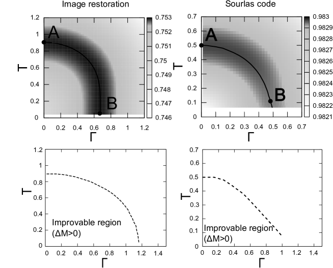
Figure 1: Upper two panels show the value of overlap $M$ as a function of controlled parameters $T$ and $\Gamma$ for image restoration (left) and Sourlas code (right). Overlap is maximized on solid lines. Lower two panels indicate improvable $(\Delta M>0$, see the definition of $\Delta M$ in (20) and worsened regions ($\Delta M<0$) for image restoration (left) and Sourlas code (right). $\Delta M=0$ holds on dashed lines. We set the parameters to $\tau_{0}=\tau=1.0,\;h=0.9,$, and $\beta_{0}=0.9$ for the image restoration model and $J=J_{0}=1.0,$ and $p=3$ for the Sourlas code (These were taken from ours Otsubo ; Inoue_PRE ).

To quantify the performance, here we use the overlap:

$$M=\frac{1}{N}\sum_{i}\xi_{i}\overline{\xi}_{i}$$ (20)

and show the $\Gamma$-$T$ diagram with gradation in Fig.1 (upper two panels). We also display the critical line on which improvable (from estimation using conventional thermal (classical) fluctuation, $\Delta M>0$) and worsened regions are separated in Fig.1 (lower two panels), where we introduced the following quantity:

$$\Delta M(\Gamma,\Omega)=M(\Gamma,\Omega)-M(0,\Omega),$$ (21)

that is, the difference between the overlaps at $\Omega=\{T_{0},T,\alpha\equiv K/N\}$ with and without the quantum fluctuations. The solid lines in the upper two panels indicate the lines on which overlap is maximized. A peak appears in the overlap and then the location of the peak is roughly the same as that in the results for the classical case. We also plot the same quantities as in Fig. 1 for CDMA multiuser demodulator in Fig. 2.

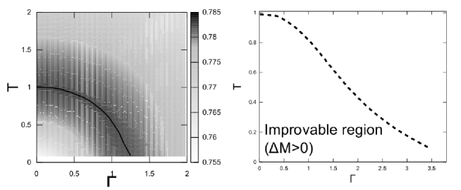
Figure 2: Overlap $M$ on $\Gamma$-$T$ plane for $T_{0}=1.0$ and $\alpha=2.0$ (left) for CDMA multiuser demodulator. Solid line indicates location of peak in $M$. The right panel shows Improvable regions ($\Delta M>0$) in $T$-$\Gamma$ (left) $T_{0}=1.0$. Dashed lines indicate border at which $\Delta M=0$ holds for $\alpha=K/N=2$ (These were taken from ours Otsubo2 ).

From these figures, we might conclude that the equivalence of two distinct fluctuations is observed even in the applications to various problems in computer science.

5 Dynamics, quantum phase transitions, across critical point

As we already mentioned, quantum Monte Carlo method is very powerful, however, when we simulate the quantum system at zero temperature in which quantum effect is essential, we encounter some technical difficulties. Therefore, it might be useful to look for exactly (analytically) solvable model to investigate the dynamical properties without computer simulations. Here we show that we can describe the quantum Monte Carlo dynamics by means of macroscopic order parameter flows for some class of infinite range models Inoue2010 . Note that such order parameter flows for classical Monte Carlo dynamics were already obtained in Coolen1988 . We also should note that Bapst and Semerjian recently extended the mean-field quantum dynamics Bapst .

Here we consider the pure ferromagnetic Ising model put in a transverse field. In terms of quantum Monte Carlo method, the master equation for the probability of the microscopic states on the $k$-th Trotter slice $p_{t}(\mbox{\boldmath$\sigma$}_{k})$ is written by

$$\frac{dp_{t}(\mbox{\boldmath$\sigma$}_{k})}{dt} = \sum_{i=1}^{N}\left[p_{t}(F_{i}^{(k)}(\mbox{\boldmath$\sigma$}_{k}))w_{i}(F_{i}^{(k)}(\mbox{\boldmath$\sigma$}))-p_{t}(\mbox{\boldmath$\sigma$}_{k})w_{i}(\mbox{\boldmath$\sigma$}_{k})\right]$$ (22)

$$F_{i}^{(k)}(\mbox{\boldmath$\sigma$}_{k}) \equiv (\sigma_{1}(k),\cdots,-\sigma_{i}(k),\cdots,\sigma_{N}(k))$$ (23)

where $p_{t}(\mbox{\boldmath$\sigma$}_{k})$ denotes a probability that the system in the $k$-th Trotter slice is in a microscopic state $\mbox{\boldmath$\sigma$}_{k}$ at time $t$.

The probability that the system is described by the magnetizationon each Trotter slice $m_{k}=N^{-1}\sum_{i}\sigma_{i}(k)$ at time $t$ is given in terms of the probability $p_{t}(\mbox{\boldmath$\sigma$}_{k})$ for a given realization of the microscopic state as $P_{t}(m_{k})=\sum_{\mbox{\boldmath$\sigma$}_{k}}p_{t}(\mbox{\boldmath$\sigma$}_{k})\delta(m_{k}-m_{k}(\mbox{\boldmath$\sigma$}_{k}))$. After simple algebra, we have

$$\frac{dP_{t}(m_{k})}{dt} = \frac{\partial}{\partial m_{k}}\{m_{k}P_{t}(m_{k})\}-\frac{\partial}{\partial m_{k}}\{P_{t}(m_{k})\langle\sigma(k)\rangle_{path}\}$$ (24)

where $\langle\sigma(k)\rangle_{path}$ is exactly the same form as the right hand hand side of equation (19). In order to obtain the deterministic equation of order parameter, we should use the static approximation $m_{k}=m,\,\forall(k)$. Then, equation (24) leads to

$$\frac{dP_{t}(m)}{dt} = \frac{\partial}{\partial m}\{mP_{t}(m)\}-\frac{\partial}{\partial m}\left\{P_{t}(m)\frac{Jm}{\sqrt{(Jm)^{2}+\Gamma^{2}}}\tanh\sqrt{(Jm)^{2}+\Gamma^{2}}\right\}.$$ (25)

Finally, substituting the form $P_{t}(m)=\delta(m-m(t))$ into (25) and making the integral by part with respect to $m$ after multiplying itself $m$, we obtain the following deterministic equation.

$$\frac{dm}{dt} = -m+\frac{Jm}{\sqrt{(Jm)^{2}+\Gamma^{2}}}\tanh\beta\sqrt{(Jm)^{2}+\Gamma^{2}}$$ (26)

It is easy to see that the steady state $dm/dt=0$ is nothing but the equilibrium state described by the equation of state $m=Jm\{\sqrt{(Jm)^{2}+\Gamma^{2}}\}^{-1}\tanh\beta\sqrt{(Jm)^{2}+\Gamma^{2}}$.

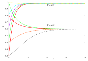
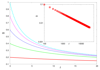
Figure 3: Typical behaviour of zero-temperature dynamics described by (26) with $\beta=\infty$ far from the critical point $\Gamma_{c}=J=1$ of quantum phase transition (left). The right panel denotes the zero-temperature dynamics at the critical point. The inset shows the log-log plot of $m(t)$ indicating that the dynamical exponent in the critical slowing down is $\nu=1/2$ (These figures were taken from ours Inoue2010 ).

In Fig. 3 (left), we plot the typical behaviour of zero-temperature dynamics (equation (26) with $\beta=\infty$) far from the critical point $\Gamma_{c}=J=1$ of quantum phase transition. We easily find that the dynamics exponentially converges to the steady state. The right panel denotes the zero-temperature dynamics at the critical point. The inset shows the log-log plot of $m(t)$ indicating critical slowing down $m(t)\simeq t^{-1/2}$.

To confirm the validity of static approximation, we can carry out computer simulation for finite size system having $N=400$ spins. We observe the time evolving process of the histogram $P(m_{k})$ which is calculated from the $M=N=400$ copies of the Trotter slices. We show the result in Fig. 4. In this simulation, we chose the initial configuration in each Trotter slice randomly and choose the inverse temperature $\beta=2$ for $\Gamma=0.5$ and $\Gamma=0.6$. From both panels in Fig. 4, we find that at the beginning, the $P(m_{k})$ is distributed due to the random set-up of the initial configuration, however, the fluctuation rapidly (eventually) shrinks to the delta function. After that, the $P(m_{k})$ evolves as a delta function with the peak located at the value of spontaneous magnetization which is explicitly indicated in the inset of each panel. Hence, we are numerically confirmed that the static approximation is valid for the pure ferromagnetic infinite range Ising model (see also Inoue2010 for random field Ising model).

As we mentioned in introduction, the gap decreases to zero at the critical point Young , which means that adiabatic evolution across the critical point is impossible to be described analytically even in the infinite range model. However, we may discuss scaling behavior across the critical point (quenching) (e.g. Chandran ; Heyl ) using the infinite range model.

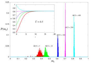
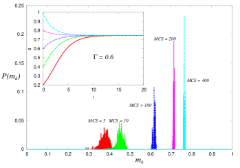
Figure 4: Time evolution of the distribution $P(m_{k})$ calculated for finite size system with $N=M=400$. We choose the inverse temperature $\beta=2$ for $\Gamma=0.5$ (left) and $\Gamma=0.6$ (right). The inset in each panel denotes the deterministic flows of spontaneous magnetization calculated by (26) for corresponding parameter sets (These figures were taken from Inoue2010 ).

6 Summary

In this paper, we showed the relationship between the probabilistic information processing and theory of quantum spin glasses through the analysis of the infinite-range model. In classical spin glass, the infinite range model, that is, Sherrington-Kirkpatrick model Sherrington is an exactly solved with in the Parisi scheme Mezard2 . This fact is very powerful because a lot of problems concerning computer science could be described by the variant of the SK model. However, as we discussed, for quantum extension of the solvable spin glass put in a transverse filed, we do not have yet exact solution due to the absence of alternative way of the static approximation. Therefore, the existence of replica symmetry breaking at low temperature has not yet been cleared Ray . The static approximation is also required when we discuss the dynamics of quantum Monte Carlo analytically. Overcoming of this difficultly might be addressed as the most important issue in this research field.

Acknowledgements

The author gratefully acknowledges his friends and colleagues Y. Otsubo, K. Nagata, M. Okada, S. Suzuki, Y. Saika, A. Das, A. Chandra, S. Dasgupta, P. Sen, A. Dutta, S. Sharma and B. K. Chakrabarti for collaboration on this research topic. This study was financially supported by Grant-in-Aid for Scientific Research (C) of Japan Society for the Promotion of Science (JSPS) No. 2533027803, Grant-in-Aid for Scientific Research (B) No. 26282089, and Grant-in-Aid for Scientific Research on Innovative Area No. 2512001313.

References

- (1) S. Suzuki, J. Inoue, and B.K. Chakrabarti, Quantum Ising Phases and Transitions in Transverse Ising Models, Lecture Notes in Physics, Vol. 862, Springer (2012).
- (2) T. Kadowaki and H. Nishimori, Phys. Rev. E 58, 5355 (1998).
- (3) E. Farhi, J. Goldstone, S. Gutmann, J. Lapan, A. Lundgren and D. Preda, Science 292, 472 (2001).
- (4) G. E. Santoro, Roman Martonak and E. Tosatti, R. Car, Science 295, 5564 (2002).
- (5) R. Harris, A. J. Berkley, M. W. Johnson, P. Bunyk, S. Govorkov, M. C. Thom, S. Uchaikin, A. B. Wilson, J. Chung, E. Holtham, J. D. Biamonte, A. Yu. Smirnov, M. H. S. Amin, and Alec Maassen van den Brink. Sign- and magnitude-tunable coupler for superconducting flux qubits. Phys. Rev. Lett. 98, 177001 (2007).
- (6) M. W. Johnson, M. H. S. Amin, S. Gildert, T. Lanting, F. Hamze, N. Dickson, R.Harris, A. J. Berkley, J. Johansson, P. Bunyk, E. M. Chapple, C. Enderud, J. P. Hilton, K. Karimi, E. Ladizinsky, N. Ladizinsky, T. Oh, I. Perminov, C. Rich, M. C. Thom, E. Tolkacheva, C. J. S. Truncik, S. Uchaikin, J. Wang, B. Wilson and G. Rose, Nature 473, 194 (2011).
- (7) S. Boixo, T. Albash, F. M. Spedalieri, N. Chancellor, and D. A. Lidar, Nature Communications 4, 2067 (2013).
- (8) J. J. Hopfield, Proc. Natl. Acad. Sci. U.S.A. 79, 2554 (1982).
- (9) D. Sherrington and S. Kirkpatrick, Phys. Rev. Lett. 35, 1792 (1975).
- (10) D.J. Amit, H. Gutfreund, and H. Sompolinsky, Phys. Rev. Lett. 55, 1530 (1985).
- (11) J. Vannimenus and M. Mezard, J. Physique Lett. 45, L1145 (1984).
- (12) M. Mézard and G. Parisi, J. Physique 47, 1285 (1986).
- (13) M. Mézard G. Parisi, and M.A. Virasoro, Spin Glass Theory and Beyond (Singapore: World Scientific 1987).
- (14) Y. Uesaka, Mathematical Foundation of Neural Computing, Kindai Kagakusha (in Japanese) (1993).
- (15) B. K. Chakrabarti, A. Das, and J. Inoue, Euro. Phys. J. B 51, 321 (2006).
- (16) A.K. Chandra, J. Inoue, and B.K. Chakrabarti, Phys. Rev. E 81, 021101 (2010).
- (17) H. Nishimori, Statistical Physics of Spin Glasses and Information Processing, (Oxford Science Publications, Oxford, 2001).
- (18) H. Nishimori and K. Y, M. Wong, Phys. Rev. E 60, 132 (1999).
- (19) K. Tanaka, J. Phys. A 35, R81 (2002).
- (20) J. Inoue, Phys. Rev. E 63, 046114 (2001).
- (21) E. Cohen, M. Carmi, R. Heiman, O. Hadar, A. Cohen, ‘Image restoration via ising theory and automatic noise estimation’ in IEEE Conf. Proceedings of International Symposium on Broadband Multimedia Systems and Broadcasting (BMSB), pp. 1-5 (2013).
- (22) E. Cohen, M. Shnitser, T. Avraham and O. Hadar, ‘Correction of defective pixels for medical and space imagers based on Ising Theory’, in Proceedings of SPIE 9217, Applications of Digital Image Processing XXXVII, 921713 (2014).
- (23) N. Sourlas, Nature 339, 693 (1989).
- (24) Y. Kabashima and D. Saad, Europhys. Lett. 45, 98 (1999).
- (25) T. Tanaka, Europhys. Lett. 54, 540 (2001).
- (26) H. Nishimori and Y. Nonomura, J. Phys. Soc. Jpn. 65, 3780 (1996).
- (27) M. Suzuki, Prog. Theor. Phys. 56, 2454 (1976).
- (28) D. Thirumalai, Q. Li, and T. R. Kirkpatrick, J. Phys. A 22, 3339 (1989).
- (29) T. Obuchi, H. Nishimori, and D. Sherrington, J. Phys. Soc. Jpn. 76, 054002 (2007).
- (30) P. Ray, B. K. Chakrabarti, and A. Chakrabarti, Phys. Rev. B 39, 11828 (1989).
- (31) J. R. L. de Almeida and D. J. Thouless, J. Phys. A 11, 983 (1978).
- (32) Y. Y. Goldschmidt, Phys. Rev. B 41, 4858 (1990).
- (33) Y. Y. Goldschmidt and P.-Y. Lai, Phys. Rev. Lett. 64, 2467 (1990).
- (34) J. Inoue, Quantum Spin Glasses, Quantum Annealing and Probabilistic Information Processing, Lecture Notes in Physics, Vol. 679, 259 (Springer, Berlin, 2005).
- (35) J. Inoue, Y. Saika, and M. Okada, J. Phys. Conf. Ser. 143, 012019 (2009).
- (36) Y. Otsubo, J. Inoue, K. Nagata and M. Okada, Phys. Rev. E 86 051138 (2012).
- (37) Y. Otsubo, J. Inoue, K. Nagata and M. Okada, Phys. Rev. E 90, 012126 (2014).
- (38) J. Inoue, J. Phys. Conf. Ser. 233, 012010 (2010).
- (39) A.C.C. Coolen and Th. W. Ruijgrok Phys. Rev. A 38, 4253 (1988).
- (40) V. Bapst and G. Semerjian, J. Phys. Conf. Ser. 473, 012011 (2013).
- (41) A. P. Young, S. Knysh, and V. N. Smelyanskiy, Phys. Rev. Lett. 101, 170503 (2008).
- (42) A. Chandran, A. Erez, S. S. Gubser, and S. L. Sondhi, Phys. Rev. E 86, 064304 (2012).
- (43) M. Heyl, A. Polkovnikov, and S. Kehrein, Phys. Rev. Lett. 110, 135704 (2013).