Deviations from piecewise linearity in the solid-state limit with approximate density functionals

Abstract

In exact density functional theory (DFT) the total ground-state energy is a series of linear segments between integer electron points, a condition known as “piecewise linearity”. Deviation from this condition is indicative of poor predictive capabilities for electronic structure, in particular of ionization energies, fundamental gaps, and charge transfer. In this article, we take a new look at the deviation from linearity (i.e., curvature) in the solid-state limit by considering two different ways of approaching it: a large finite system of increasing size and a crystal represented by an increasingly large reference cell with periodic boundary conditions. We show that the curvature approaches vanishing values in both limits, even for functionals which yield poor predictions of electronic structure, and therefore can not be used as a diagnostic or constructive tool in solids. We find that the approach towards zero curvature is different in each of the two limits, owing to the presence of a compensating background charge in the periodic case. Based on these findings, we present a new criterion for functional construction and evaluation, derived from the size-dependence of the curvature, along with a practical method for evaluating this criterion. For large finite systems we further show that the curvature is dominated by the self-interaction of the highest occupied eigenstate. These findings are illustrated by computational studies of various solids, semiconductor nanocrystals, and long alkane chains.

I Introduction

Kohn-Sham (KS) density functional theory (DFT) Hohenberg1964 ; Kohn1965 is a widely used first-principles approach to the many-electron problem. It is based on mapping the system of $N$ interacting electrons into a unique non-interacting system with the same ground state electron density. (Levy1982, ; Lieb1983, ) In the non-interacting system the density is determined by $n\left(\mathbf{r}\right)=\sum_{i}f_{i}\left|\psi_{i}\left(\mathbf{r}\right)\right|^{2}$ where $\psi_{i}\left(\mathbf{r}\right)$ $\left(i=1,2,...\right)$ are normalized single particle eigenstates and $f_{i}$ are the corresponding occupation numbers. The eigenstates are determined from the KS equations

$$\hat{H}\psi_{i}=\varepsilon_{i}\psi_{i},$$ (1)

where $\varepsilon_{i}$ are the (monotonically increasing) KS eigenvalues (see footnote ) and

$$\hat{H}=-\frac{1}{2}\nabla^{2}+v_{H}\left({\bf r}\right)+v_{XC}\left({\bf r}\right)+v_{ext}\left({\bf r}\right)$$ (2)

is the KS Hamiltonian (atomic units are used throughout). In Eq. (2), $v_{H}\left({\bf r}\right)$ is the Hartree potential, $v_{XC}\left({\bf r}\right)$ the exchange-correlation (XC) potential and $v_{ext}\left({\bf r}\right)$ is the external potential operating on the electrons in the interacting system. While DFT in general, and the KS equation in particular, are exact in principle, the XC potential functional is always approximated in practice and thus defines the level of theory applied.

The exact XC energy functional, $E_{XC}\left[n\right]$, from which the XC potential is derived via the relation $v_{XC}\left({\bf r}\right)=\delta E_{XC}\left[n\right]/\delta n\left({\bf r}\right)$, is known to satisfy a number of constraints (e.g., Ref. 6). One constraint, on which we focus here, is the piecewise-linearity property. (Perdew1982a, ) Perdew et al. have argued that the ensemble ground-state energy $E\left(N\right)$ as a function of electron number, $N$ where $N_{0}-1\leq N\leq N_{0}$, must be a series of linear segments between the integer electron points $N_{0}$. Within the KS formalism this requirement translates directly into a condition on the XC energy functional, $E_{XC}\left[n\right]$.

An important manifestation of piecewise-linearity is the relation between the highest occupied eigenvalue, $\varepsilon_{H}$, and the ionization potential, $I(N_{0})\equiv E\left(N_{0}\right)-E\left(N_{0}-1\right)$. These considerations have been originally developed for finite systems; infinite systems are discussed in detail below. For the exact functional, piecewise-linearity dictates that $I=-dE/dN$. In addition, Janak’s theorem (Janak1978, ) states that for any (exact or approximate) XC functional, the highest occupied eigenvalue obeys

$$\varepsilon_{H}=\frac{dE_{KS}}{df_{H}},$$ (3)

where $E_{KS}$ is the KS estimate for the energy of the interacting system. For any change in electron number $N$, the same change occurs in $f_{H}$, the occupation number of the highest occupied eigenstate of the non-interacting system. Thus we find the result $I=-\varepsilon_{H}$ for a KS theory which uses the exact XC functional (i.e. for which $E_{KS}=E$). This exact condition, known as the ionization potential theorem, (Perdew1982a, ; Levy1984a, ; Almbladh1985, ; Perdew1997, ) can be conveniently restated in terms of the energy curvature, $C$, defined as the second derivative of the total energy functional with respect to the fractional electron number,

$$C=\frac{d^{2}E}{dN^{2}}=\frac{d^{2}E_{KS}}{df_{H}^{2}}=\frac{d\varepsilon_{H}}{df_{H}},$$ (4)

where Janak’s theorem has been used in the third equality. Fulfillment of piecewise-linearity implies that $C=0$, i.e. that the curvature is zero.

Despite the importance of piecewise-linearity, it has long been known that standard application of commonly used functional classes, such as the local density approximation (LDA), the generalized gradient approximation (GGA), or conventional hybrid functionals with a fixed fraction of Fock exchange (e.g. Ref. 12), grossly disobeys this condition. In practice, a substantial, non-zero curvature is observed. The $E_{KS}\left(f_{H}\right)$ curve is typically strongly convex (see, e.g. 13; 14; 15; 16; 17; 18; 19; 20; 21; 22) and, correspondingly, $-\varepsilon_{H}$ can underestimate $I$ by as much as a factor of two. (Tozer1998, ; Allen2002, )

The lack of piecewise-linearity in approximate functionals further affects the prediction of the fundamental gap, $E_{g}$, defined as the difference between the minimum energy needed for electron removal and the maximum energy gained by electron addition. Even with the exact functional, the KS eigenvalue gap, $\varepsilon_{L}-\varepsilon_{H}$ (where $\varepsilon_{L}$ is the energy of the lowest unoccupied eigenstate), need not equal $E_{g}$ (Perdew1983, ; Sham1983, ). Instead,

$$E_{g}=\varepsilon_{L}-\varepsilon_{H}+\Delta_{XC},$$ (5)

where $\Delta_{XC}$ is the derivative discontinuity (Perdew1982a, ; Perdew1985, ; Sagvolden2008, ; Cohen2014Dramatic, ) - a spatially-constant “jump” in the XC potential as the integer number of particles is crossed. This discontinuity is itself a consequence of piecewise linearity: The discontinuous change of slope in the energy as a function of electron number must also be reflected in the energy computed from the KS system. Some of it is contained in the kinetic energy of the non-interacting electrons, but the rest must come from a discontinuity in the XC potential. (Perdew1982a, ) Note that within the generalized KS (GKS) scheme (see footnote ) part of the discontinuity in the energy may also arise from a non-multiplicative (e.g., Fock) operator. (Seidl1996, ; KronikKuemmel2008, ; Yang2012, ) Therefore the derivative discontinuity in the XC potential may be mitigated and in some cases even eliminated. Eisenberg2009 ; Stein2010 ; Kronik2012 ; Yang2012

For any approximate (G)KS scheme, $E_{g}$ can be expressed as (Stein2012, )

$$E_{g}=\varepsilon_{L}-\varepsilon_{H}+\frac{1}{2}\left(C^{hole}+C^{elec}\right)+\Delta_{XC},$$ (6)

where $C^{hole}$ and $C^{elec}$ are the curvatures associated with electron removal and addition, respectively. The curvatures act as “doppelgänger” for the missing derivative discontinuity. Whereas in the exact functional all curvatures are zero and the difference between $E_{g}$ and the eigenvalue gap is given solely by $\Delta_{XC}$, for standard approximate (semi-)local (LDA and GGA) or hybrid functionals, employed in the absence of ensemble corrections, $\Delta_{XC}$ is zero and the addition of the average curvature compensates quantitatively for the missing derivative discontinuity term. (Stein2012, ) In the most general case, both a remaining curvature and a remaining derivative discontinuity will contribute to the difference between $E_{g}$ and $\varepsilon_{L}-\varepsilon_{H}$.

For small finite systems, the criterion of piecewise linearity (i.e., zero curvature) has been employed to markedly improve the connection between eigenvalues and ionization potentials or fundamental gaps, and often also additional properties, in at least four distinct ways: (i) In the imposition of various corrections on existing underlying exchange-correlation functionals; (cococcioni2005linear, ; LanyZunger2009, ; Dabo2010, ; Stein2012, ; ChaiChen2013, ; Ferretti2014, )(ii) In first-principles ensemble generalization of existing functional forms; (kraisler2013piecewise, ; kraisler2014fundamental, ) (iii) In the construction and evaluation of novel exchange-correlation functionals; (Kuisma2010, ; ArmientoKuemmel2013, ) And (iv) in non-empirical tuning of parameters within hybrid functionals, (Sai2011, ; Atalla2013, ) especially range-separated ones. (Stein2010, ; Baer2010a, ; Kronik2012, ; Srebro2014, )

Unfortunately, this remarkable success of the piecewise-linearity criterion does not easily transfer to large systems possessing delocalized orbitals. For example, for a LDA treatment of hydrogen-passivated silicon nanocrystals (NCs), the fundamental gap computed from total energy differences approaches the KS eigenvalue gap with increasing NC size. (Ogut1997, ; Godby1998, ) As mentioned above, for LDA $\Delta_{XC}=0$. Taken together with Eq. (6), this implies that as system size grows the average curvature becomes vanishingly small and piecewise linearity is approached. (Mori-Sanchez2008a, ) Despite this, the ionization potential obtained this way does not agree with experiment. (salzner2010modeling, )

This limitation is intimately related to the vanishing ensemble correction to the band gap of periodic solids (kraisler2014fundamental, ) and even to the failure of time-dependent DFT for extended systems (Onida2002, ; IzmaylovScuseria2008, ). This is a disappointing state of affairs, because the zero curvature condition that has been used so successfully for small finite systems, both diagnostically and constructively, appears to be of little value for extended systems, even though the problem it is supposed to diagnose is still there.

In this article, we take a fresh look at this problem, by considering the evolution of curvature with system size. We approach the bulk limit in two different ways: (i) Calculations for an increasingly large but finite system (namely nanocrystals and molecular chains). (ii) Calculations for a crystal represented by an increasingly large reference cell with periodic boundary conditions. We show that in both cases the curvature approaches zero. However, it doesn’t do so in same fashion, due to the presence of a compensating background charge in the periodic system. Based on these findings, we present a new criterion for functional construction and an assessment derived from the size-dependence of the curvature, along with a practical method for evaluation this criterion. We further show that the curvature for large finite systems is dominated by the self-interaction of the highest occupied eigenstate. These findings are illustrated by computational studies of semiconductor NCs and long alkane chains.

II Energy curvature in large finite systems

II.1 General considerations

We first examine finite systems, in which, as noted above, curvature effects have been already studied extensively. As a first step in our general theoretical considerations, we express the curvature of a finite system as the rate of change in the energy of the highest-occupied KS-eigenstate as an electronic charge $q$ is removed or added (see footnote ) to the system:

$$C=\frac{d\varepsilon_{H}}{dq}=\left\langle\psi_{H}\left|\frac{d\hat{H}}{df_{H}}\right|\psi_{H}\right\rangle.$$ (7)

The first equality is a restatement of Eq. (4), combined with the fact that the removed (added) charge is taken from (inserted into) the highest occupied eigenstate $\psi_{H}$, (see footnote ) while the second is due to the Hellmann-Feynman theorem (Hellman1937, ; Feynman1939, ). As the derivative in Eq. (7) is applied only to the terms of the Hamiltonian $\hat{H}$ that are functionals of the density, $n\left({\bf r}\right)$, we can write the curvature as (Salzner2009, )

$$C=\int n_{H}\left(\mathbf{r}\right)\int\left[\frac{1}{|{\bf r}-\mathbf{r}^{\prime}|}+f_{XC}\left({\bf r},\mathbf{r}^{\prime}\right)\right]\frac{dn\left(\mathbf{r}^{\prime}\right)}{df_{H}}d^{3}r^{\prime}\mathrm{d}^{3}r,$$ (8)

where $f_{XC}\left({\bf r},{\bf r^{\prime}}\right)=\delta^{2}E_{XC}[n]/\delta n(\mathbf{r})\delta n(\mathbf{r}^{\prime})$ is the exchange-correlation kernel and $n_{i}\left(\mathbf{r}\right)\equiv\left|\psi_{i}\left({\bf r}\right)\right|^{2}$ is the density of the $i^{th}$ KS eigenstate. Using the fact that the electron density is given by $n\left({\bf r}\right)=\sum_{i}f_{i}n_{i}\left(\mathbf{r}\right)$, it follows that

$$\frac{dn\left({\bf r}\right)}{df_{H}}=n_{H}\left({\bf r}\right)+n_{relax}\left(\mathbf{r}\right),$$ (9)

where the first term on the right hand side is the density of the highest occupied KS eigenstate and the second term, $n_{relax}\left(\mathbf{r}\right)\equiv\sum_{i}f_{i}\left(dn_{i}\left(\mathbf{r}\right)/df_{H}\right)$, describes the eigenstate density relaxation upon charge removal/addition. The curvature can therefore be expressed as:

$$C =\iint\frac{n_{H}\left(\mathbf{r}\right)n_{H}\left(\mathbf{r}^{\prime}\right)}{|{\bf r}-\mathbf{r}^{\prime}|}d^{3}r^{\prime}d^{3}r$$ (10)

$$\,\,+\iint\frac{n_{H}\left(\mathbf{r}\right)n_{relax}\left(\mathbf{r}^{\prime}\right)}{\left|\mathbf{r}-\mathbf{r}^{\prime}\right|}d^{3}r^{\prime}d^{3}r+C_{XC}.$$

The first term in Eq. (10) is twice the electrostatic interaction energy of $n_{H}\left(\mathbf{r}\right)$ with itself; the second term is twice the electrostatic interaction energy between $n_{H}\left(\mathbf{r}\right)$ and the relaxation density, $n_{relax}\left(\mathbf{r}\right)$; the last term,

$$C_{XC}=\iint n_{H}\left(\mathbf{r}\right)\left[n_{H}\left(\mathbf{r}^{\prime}\right)+n_{relax}\left(\mathbf{r}^{\prime}\right)\right]f_{XC}\left({\bf r},\mathbf{r}^{\prime}\right)d^{3}r^{\prime}d^{3}r,$$ (11)

is the contribution of the exchange-correlation kernel to the curvature. As discussed in the introduction, for the exact exchange-correlation functional the curvature is identically zero and therefore the two electrostatic (Hartree) terms must be canceled out by the exchange-correlation kernel term.

In the LDA, the approximate exchange-correlation kernel is of the form: Petersilka1996 $f_{XC}^{LDA}\left(\mathbf{r},\mathbf{r}^{\prime}\right)=\delta\left(\mathbf{r}-\mathbf{r}^{\prime}\right)\tilde{f}_{XC}^{LDA}\left(n\left({\bf r}\right)\right)$. The expression for the exchange-correlation contribution to the curvature then simplifies to

$$C_{XC}^{LDA}=\int n_{H}\left(\mathbf{r}\right)\left[n_{H}\left(\mathbf{r}\right)+n_{relax}\left(\mathbf{r}\right)\right]\tilde{f}_{XC}^{LDA}\left(n\left({\bf r}\right)\right)d^{3}r,$$ (12)

which does not generally cancel the Hartree terms in Eq. (10). This is consistent with the above-mentioned deviations from piecewise-linearity found in LDA calculations of small molecules.

II.2 Energy curvature in large finite three-dimensional systems

To gain insight into the behavior of curvature as a function of system size, we first consider an electron gas consisting of $N_{e}$ electrons distributed uniformly in a finite volume $\Omega$ with periodic boundary conditions. For such a system, $n_{i}\left(\mathbf{r}\right)=\frac{1}{\Omega}$ and there is no eigenstate relaxation i.e. $n_{relax}(\mathbf{r})=0$. Therefore the general curvature expression of Eq. (10) includes only the electrostatic self-interaction and XC terms and, using LDA, can be simplified to

$$\bar{C} =\frac{1}{\Omega^{2}}\iint_{\Omega}\frac{1}{|{\bf r}-\mathbf{r}^{\prime}|}d^{3}r^{\prime}d^{3}r+\frac{\tilde{f}_{XC}^{LDA}\left(n\right)}{\Omega}$$ (13)

$$=\frac{\bar{D}}{\Omega^{1/3}}+\frac{\tilde{f}_{xc}^{LDA}\left(n\right)}{\Omega},$$

where we have used the fact that for a given uniform density, $n=N_{e}/\Omega$, the LDA XC kernel is constant. Note that the bar over $C$ and $D$ is used to denote quantities relating to a uniform electron density. The first term in Eq. (13) is twice the electrostatic self-interaction energy of a unit charge, which is characterized by a volume-independent shape factor $\bar{D}=\frac{1}{\Omega^{5/3}}\iint_{\Omega}\frac{1}{|{\bf r}-{\bf r^{\prime}}|}\mathrm{d}^{3}r^{\prime}d^{3}r$. Analytical integration yields $\bar{D}=\frac{6}{5}(\frac{4\pi}{3})^{1/3}E_{H}a_{0}\approx$52.5 $eVa_{0}$ for a sphere, where $E_{H}$ and $a_{0}$ are the atomic Hartree and Bohr units for energy and length, respectively. For a cube and a parallelepiped of the shape of a diamond primitive cell, numerical integration yields $\bar{D}\approx$51.2 $eVa_{0}$ and 49.0 $eVa_{0}$, respectively, with the former value in agreement with electrostatic energy calculations reported in Ref. 61.

Clearly, the curvature of this uniform-electron-gas based example decays to zero as the system size increases. Specifically, in the limit of an infinitely large uniform electron gas limit, where LDA is an exact result, the exact DFT condition of zero curvature is indeed obeyed. However, for a uniform electron gas confined to a finite volume, the LDA is not exact and therefore non-zero curvature is to be expected.

In Eq. (13), the curvature for large systems is dominated by the $\bar{D}\Omega^{-1/3}$ term, which arises from the electrostatic self-interaction of the highest occupied eigenstate. It stands to reason that such a term, with a general prefactor $D$, can be expected not just for this idealized system, but also for realistic large but finite systems for which LDA is a reasonable approximation.

To test this hypothesis, we focused on the elemental group IV solids - diamond, silicon, and germanium - for which LDA is well-proven to be a good approximation for ground-state properties. Godby1987 ; Chelikowsky1992 For each solid, we constructed a set of increasingly large nanocrystals in two stages. First, we replicated the primitive unit cell of the bulk crystal an equal number of times in each of the lattice vector directions, using the experimental lattice constant, thereby creating a finite but periodic supercell. Second, we removed unbound atoms and passivated any remaining dangling bonds with hydrogen atoms. In this way, hydrogen-passivated NCs containing up to 325 Si, C, or Ge atoms, as well as a passivation layer containing up to 300 H atoms, were formed. For each of the NCs constructed this way, we calculated the LDA energy curvature for both charge removal and charge addition. All calculations were performed using NWCHEM (Valiev2010, ) with the cc-PVDZ basis set for the smaller NCs and the STO-3G basis set for the larger NCs. The curvature was estimated by a finite difference approximation to Eq. (4), $C=\Delta\varepsilon_{H}/\Delta f_{H}$, where we calculated $\varepsilon_{H}$ for the neutral system and for systems where an incremental small fractional charge was removed from, or added to, the entire system.

The resulting curvature for each of the systems studied is shown in Fig. 1, as a function of $\Omega^{-\frac{1}{3}}$. Clearly, in the limit of large system volume, $\Omega$, all three compounds exhibit the limiting form expected, i.e., a curvature given by $C=D\Omega^{-1/3}$, for both electron removal and addition. Furthermore, by fitting our results for NCs with edges larger than $14a_{0}$ to the expected dependence, we obtained $D\approx 43.5eVa_{0}$ for all three materials. This “universal value” is reasonable in light of the fact that the highest occupied eigenstate for all three materials has a similar spatial distribution, making the Hartree self-interaction contribution similar. Moreover, it deviates from the ideal uniform-electron-gas parallelepiped by only $\sim$20%, a difference that can be attributed to the non-uniform structure of the highest occupied eigenstate obtained within LDA (see Eq. (10) above). For smaller nanocrystals, the term scaling as $\Omega^{-1}$ is non-negligible and therefore the curvature departs from the ideal $\Omega^{-1/3}$ behavior, as observed in Fig. 1. Therefore, we conclude that the curvature expression given by the right-hand side of Eq. (13), derived for the uniform electron gas, is indeed applicable also for realistic systems possessing delocalized electronic states and that the self-repulsion term dominates the curvature as the system grows.

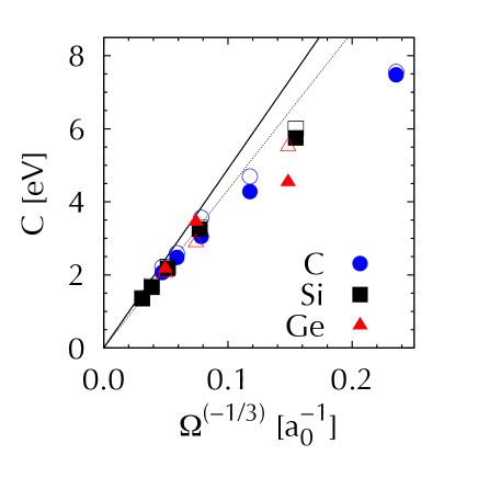
Figure 1: Curvature, $C$, obtained within the local density approximation for electron removal (solid symbols) or addition (hollow symbols) for diamond (blue circles), silicon (black squares), and germanium (red triangles) nanocrystals, as a function of $\Omega^{-\frac{1}{3}}$, where $\Omega$ is the nanocrystal volume. The dotted line represents a least-squares fit to the asymptotic dependence. The solid line represents the asymptotic dependence expected from Eq. (13) for a uniform electron gas of the same size and shape as the nanocrystals.

Interestingly, further support for the limiting $D\Omega^{-1/3}$ dependence of the curvature is obtained from the results of past LDA-based studies of the quantum size effect in spherical silicon (Ogut1997, ) and germanium (Melnikov2004, ) nanocrystals. In these studies, the difference between the fundamental gap, computed from total energy differences of the anionic, neutral, and cationic system, was compared to the KS eigenvalue gap. The difference was observed Ogut1997 ; Godby1998 ; Melnikov2004 to scale as $\sim\Omega^{-1/3}$. This observation is easily explained within our theory as a direct consequence of the non-zero curvature: (Stein2012, ) Eq. (6) shows that for (semi-)local functionals (without an explicit derivative discontinuity), the difference between the fundamental and the KS eigenvalue gap is in fact equal to the average curvature for electron addition and removal and must exhibit the same trends as a consequence. This conclusion is further supported by the value of $D=39.5\,eVa_{0}$ and $D=41.1\,eVa_{0}$, deduced for the spherical silicon and germanium NCs, respectively, from the data of Ref. 50 and Ref. 65. These values are indeed very close to the value of $D=43.5\,eVa_{0}$ which we obtained above from explicit curvature calculations for the diamond-structured NCs. Note that the change in shape does not cause a significant difference in the value of $D$, consistent with our uniform electron gas calculations.

II.3 Energy curvature in large finite one-dimensional systems

The above-demonstrated dominance of the electrostatic term in the size-dependence of the curvature suggests that it must be strongly influenced by dimensionality. To test this, we again consider twice the Hartree energy as given in Eq. (10), evaluated for a unit-charge uniform electron gas, confined to a cylinder of length $L$ and radius $d$ such that $L\gg d$, as an approximation for the curvature of a long but finite one-dimensional system. This energy can be computed analytically (ciftja2012, ) to obtain:

$$C\approx\frac{2}{L}\ln\left(2e^{-3/4}\frac{L}{d}\right),\quad L\gg d.$$ (14)

This indicates that, as in the three-dimensional case, the curvature vanishes as the system grows arbitrarily long - an observation also consistent with the results of Mori-Sánchez et al. for hydrogen chains Mori-Sanchez2008a . However, the curvature does not decay as $L^{-1}$, as perhaps could be naively expected, but rather as $L^{-1}\ln\left(\frac{2e^{-3/4}L}{d}\right)$. The relaxation and exchange-correlation terms are expected to scale as $L^{-1}$. However they do not significantly affect the curvature when $L>50a_{0}$, as for very large $L$ the logarithmic term dominates the $L^{-1}$ term.

To test whether this prediction carries over to realistic one-dimensional systems, we considered alkane chains of increasing length, $L$, whose width $d$ is fixed by definition (see inset of Fig. 2). These alkane chains provide a useful model of a quasi-one-dimensional system that is well-described by LDA. (Segev2006, ) We investigated chains containing up to 240 C atoms and again used NWCHEM (Valiev2010, ) with the cc-PVDZ and the STO-3G basis sets. The computed curvature for electron removal is shown in Fig. 2, as a function of $a_{0}/L$, and compared with the prediction of Eq. (14). Clearly, for large $L$ the curvature is once again very well approximated by the electrostatic self-interaction of a uniformly smeared unit charge.

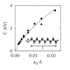
Figure 2: Curvature, $C$, obtained within the local density approximation for electron removal from alkane chains, as a function of $a_{0}/L$, where $L$ is the chain length. The line represents the asymptotic dependence expected from Eq. (14) for a unit-charge uniform electron gas of the same length as the chain and a radius of $d=2a_{0}$. Triangles and diamonds represent data obtained using the cc-PVDZ and STO-3G basis sets, respectively. Inset: the hexane molecule as an example of an alkane chain, with $d$ and $L$ shown explicitly.

III Energy curvature in periodic systems

III.1 General Considerations

In solid-state physics, it is common practice to employ periodic boundary conditions for the description of crystalline solids. Ashcroft2005 To understand the bulk limit of curvature calculations in such a scenario, we consider a reference cell of total volume $\Omega_{RC}$, containing $N$ repeating unit cells (with unit cell volume $\Omega_{UC}$), using Born - von Karman periodic boundary conditions. Ashcroft2005 In other words, the reference cell is treated as a finite but topologically periodic system. (kraisler2014fundamental, ) In such a system, the infinite bulk limit is approached with increasing size of the reference cell.(see footnote )

To compute the curvature, we remove (or add) an electronic charge $Q_{RC}$ from (or to) the reference cell, denoted below by a “hole” (or “elec”) superscript, where appropriate. We focus mostly on electron removal for simplicity. Owing to the periodic boundary conditions, electron removal from the reference cell implies removal of the same charge from each of its periodic images. As there are an infinite number of repeated reference cells, the removed electronic charge is effectively infinite, leading to divergences in the Coulomb potential. Therefore, a uniform compensating positive charge, of density $Q_{RC}/\Omega_{RC}$, is introduced to the reference cell. This keeps the infinite periodic crystal neutral and avoids the divergent behavior. (Ihm1979, ; Sharma2008, )

As before, the curvature $C_{RC}$, defined with respect to the reference cell, is computed as the rate of change of the highest occupied KS-eigenvalue with respect to removed charge, $C_{RC}=d\varepsilon_{H}/dQ_{RC}$. By construction (and assuming no symmetry breaking), the hole formed by charge removal exhibits a periodic structure commensurate with the repeating unit-cell and therefore $Q_{RC}=NQ_{UC}$, where $Q_{UC}$ is the charge removed from each of the $N$ unit cells that comprise the reference cell. In the limit of large $N$, $\varepsilon_{H}$ is expected to become independent of the size of the reference cell, i.e., of $N$. Therefore

$$C_{RC}=\frac{d\varepsilon_{H}}{dQ_{RC}}=\frac{1}{N}\frac{d\varepsilon_{H}}{dQ_{UC}}\equiv\frac{C_{UC}}{N},$$ (15)

where $C_{UC}\equiv d\varepsilon_{H}/dQ_{UC}$ is the “unit-cell curvature”, which in the limit of large $N$ is independent of the reference cell size (see footnote ).

Clearly, the curvature $C_{RC}$ for the infinite crystal does depend on the reference cell size. As the reference cell grows ($N\to\infty$, $\Omega_{RC}\to\infty$), we find $C_{RC}\rightarrow 0$ for any underlying functional. This result should be contrasted with the exact DFT condition of piecewise linearity, where the curvature given by Eq. (15) should be strictly zero for any reference cell size and not just in the infinite cell limit. In other words, as for the NCs, in the infinite system limit piecewise-linearity is obtained irrespective of the underlying XC functional and therefore does not provide useful information for functional construction or evaluation. However, in the exact theory we also expect $C_{UC}=0$. Therefore, a non-vanishing unit-cell curvature, $C_{UC}$, represents a measure of the spurious XC functional behavior even in periodic infinite solids and may prove useful in future analysis.

III.2 LDA calculations of topologically periodic reference cells

To examine the considerations and conclusions of the previous section, we performed LDA calculations for increasingly large periodic reference cells of selected semiconductors and insulators, using the LDA-optimized lattice vectors of a neutral unit cell (see footnote ).

As mentioned above, the reference cell is considered to be finite but topologically periodic. Therefore, all calculations are carried out using only the single $k$-point (at $\Gamma$). This makes curvature calculations straightforward both conceptually and practically, as charge is removed from the highest occupied KS eigenstate as in the finite-system calculations above. The energy derivatives needed for the evaluation of the curvature (Eq. (15)) were calculated using finite differences of the highest occupied energy eigenvalue, $\varepsilon_{H}$, for the neutral and incrementally charged reference cell.

The results of such calculations for increasingly large reference cells of diamond and silicon are summarized in Fig. 3. (see footnote ) As shown in the top panel of Fig. 3, the reference cell curvature indeed decreases monotonically and vanishes in the large $N$ limit, in agreement with the above theoretical considerations. At the same time, the bottom panel of Fig. 3 shows that the unit cell curvature is not zero and for large $N$ approaches a constant, material-dependent value, such that Eq. (15) is obeyed.

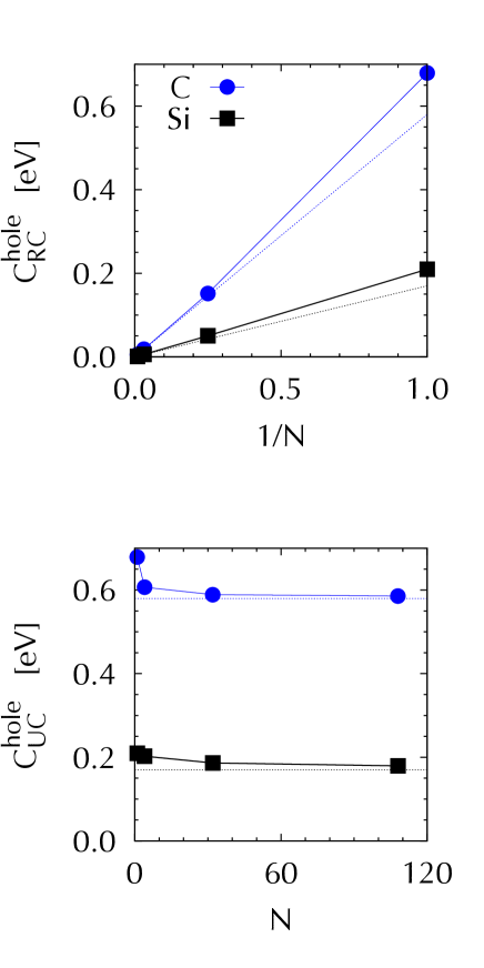
Figure 3: Computed charge removal curvature for silicon (black squares) and diamond (blue circles) crystals: (Top) Reference cell curvature, $C_{RC}^{hole}$, as a function of $N^{-1}$. (Bottom) unit cell curvature, $C_{UC}^{hole}$, as a function of $N$, where $N$ is the number of primitive unit-cells in the reference cell. Solid Lines are a guide for the eye. Dotted lines represent the asymptotic dependence on $N$ (Top), or the converged values of $C_{UC}$ (Bottom), obtained through Brillouin-zone sampling described in Sec. III.4.

III.3 Finite versus periodic cell: A seeming paradox and its resolution

In the limit of an arbitrarily large system, one would expect surface effects to be negligible and so, naively, that the limiting behavior of large periodic and non-periodic systems to be the same. However, we already showed both analytically and numerically that in fact the limiting behavior is not the same. For the finite system, the curvature asymptotically scales as $\Omega^{-1/3}$, where $\Omega$ is the volume of the finite, non-periodic system, whereas for the topologically periodic system the curvature asymptotically scales as $\Omega_{RC}^{-1}$, where $\Omega_{RC}$ is the reference cell volume.

This apparent paradox can be reconciled by recalling that in a periodic system, electron addition/removal must be accompanied by the addition of a compensating, uniformly distributed background charge of opposite sign, so as to avoid divergence of the Coulomb potential and energy. (Ihm1979, ) For a non-periodic system, however, no compensating charge is necessary. This background charge strongly affects curvature considerations.Sharma2008 To understand why, consider that if surface effects are neglected then Eq. (10), developed above for non-periodic systems, can be applied to the reference cell of a periodic system. However, while $n_{relax}$ integrates to zero in the reference cell, $n_{H}$ integrates to 1. Therefore, $n_{H}$ must be replaced by a background-neutralized density, $\rho_{H}\left(\mathbf{r}\right)\equiv n_{H}\left(\mathbf{r}\right)-\frac{1}{\Omega_{RC}}$, before it can be inserted in Eq. (10). Therefore, Eq. (10) yields the following expression for the curvature in the periodic case, $C^{periodic}$:

$$C^{periodic} =\iint_{\Omega_{RC}}\frac{\rho_{H}\left(\mathbf{r}\right)\rho_{H}\left(\mathbf{r^{\prime}}\right)}{|{\bf r}-\mathbf{r}^{\prime}|}d^{3}r^{\prime}d^{3}r$$ (16)

$$\,\,+\iint_{\Omega_{RC}}\frac{\rho_{H}\left(\mathbf{r}\right)n_{relax}\left(\mathbf{r^{\prime}}\right)}{\left|\mathbf{r}-\mathbf{r}^{\prime}\right|}d^{3}r^{\prime}d^{3}r+C_{XC}.$$

With all densities being unit-cell periodic, we can define $\tilde{n}_{j}\left(\mathbf{G}\right)=\frac{1}{\Omega_{UC}}\int_{\Omega_{UC}}n_{j}\left(\mathbf{r}\right)e^{i\mathbf{G}\cdot\mathbf{r}}d^{3}r$ as the Fourier-component of $n_{j}\left(\mathbf{r}\right)$ corresponding to the reciprocal unit-cell lattice vector, $\mathbf{G}$. For charge-neutral systems, the $\mathbf{G}=\mathbf{0}$ component must be zero. By noting that $\tilde{n}_{H}\left(\mathbf{G}\neq\mathbf{0}\right)=\tilde{\rho}_{H}\left(\mathbf{G\neq 0}\right)$, because the two densities differ only by a constant, we obtain:

$$C^{periodic} =4\pi\Omega_{RC}\sum_{\mathbf{G}\neq 0}\frac{\tilde{n}_{H}\left(\mathbf{G}\right)\tilde{n}_{H}\left(\mathbf{G}\right)^{*}}{G^{2}}$$ (17)

$$\,\,+4\pi\Omega_{RC}\sum_{\mathbf{G}\neq 0}\frac{\tilde{n}_{H}\left(\mathbf{G}\right)\tilde{n}_{relax}\left(\mathbf{G}\right)^{*}}{G^{2}}+C_{XC}.$$

The KS-eigenstate densities, $n_{j}\left(\mathbf{r}\right)$, are normalized over the reference cell and therefore $n_{H}\left(\mathbf{r}\right)$ and $n_{relax}\left(\mathbf{r}\right)$, as well as their Fourier components, must scale as $\Omega_{RC}^{-1}$. Because $\mathbf{G}$ depends only on the unit cell and is independent of $\Omega_{RC}$, Eq. (17) shows that $C^{periodic}$ scales as $\Omega_{RC}^{-1}$. Thus, we obtain a curvature that scales with inverse system volume, consistent with Eq. (15) above.

One can also compare the terms in Eq. (10) and Eq. (16), obtaining the following expression for the difference in their curvature:

$$\begin{array}[]{l}C^{finite}-C^{periodic}\\ \,\,\,\,\,\,\,\,\,\,=\iint_{\Omega_{RC}}\frac{\left(2n_{H}\left(\mathbf{r}\right)-\frac{1}{\Omega_{RC}}-n_{relax}\left(\mathbf{r}\right)\right)\frac{1}{\Omega_{RC}}}{|{\bf r}-\mathbf{r}^{\prime}|}d^{3}r^{\prime}d^{3}r.\end{array}$$ (18)

Dimensional analysis reveals that the above curvature difference scales as $\Omega_{RC}^{-1/3}$.

As discussed in Section II, $\Omega_{RC}^{-1/3}$ scaling was also obtained for the non-periodic case from the self-interaction energy of the highest-occupied eigenstate. Furthermore, because the background charge must systematically cancel the divergence in the electronic electrostatic energy, the prefactor of the $\Omega_{RC}^{-1/3}$ dependence in the above equation must be equal and opposite to that deduced from Eq. (10). Therefore, overall the $\Omega_{RC}^{-1/3}$ scaling must vanish in $C^{periodic}$ and only the $\Omega_{RC}^{-1}$ scaling remains.

To summarize, the scaling behavior of a non-periodic and a periodic system really is different, but this is not owing to topology per se, but rather stems from the effects of the uniform background charge, used in periodic calculations only. Before concluding this issue, however, two more comments are in order. First, for finite systems described with (semi-)local functionals, the scaling is self-interaction dominated and therefore positive (see, e.g., Refs. 13; 18; 17; 36). Upon elimination of this effect by the compensating background, curvature can be either positive or negative (which we show below to be the case). This is somewhat reminiscent of the behavior of the exact-exchange functional (see, e.g., Ref. 13), where self-interaction is eliminated and the curvature is typically mildly negative. Second, for periodic systems we assumed throughout that the removed/added charge is delocalized throughout the reference cell. If this is not the case, e.g., if a molecule or a localized defect is computed within a large supercell, scaling arguments no longer apply and the results will resemble those of finite systems. This explains, among other things, why a Hubbard-like $U$ term for localized states in an otherwise periodic system is indeed useful, as long as the correction is limited to the vicinity of the localized site (see, e.g., Refs.75; 37).

III.4 Brillouin zone sampling

In Section III.2 we have considered the infinite solid limit by constructing increasingly large topologically-periodic reference cells. While pedagogically useful, this procedure is too cumbersome and computationally expensive to be used for routine unit-cell curvature calculations. In practice, the infinite-solid limit is much easier to reach by using $k$-point sampling of the Brillouin zone corresponding to a single periodic unit cell. This sampling relies on Bloch’s theorem, which allows the eigenfunctions of a periodic Hamiltonian to have the same periodicity up to a phase factor. Ashcroft2005 One can then show that a single unit cell with uniform sampling of $N$ $k$-points is completely equivalent, mathematically and physically, to a reference cell comprised of $N$ unit cells within the single $k$-point ($k=0$) treatment. (Pickett1989, ) Specifically, for a semiconductor or insulator in the ground state the $n$ electrons in the unit cell occupy the lowest eigenstates, with energies $\varepsilon_{i,k}$ (where $i$ is the band index and $k$ is the $k$-point index). This is equivalent to a system with $n\times N$ electrons, i.e. a reference cell comprised of $N$ unit cells. The infinite solid limit, then, simply corresponds to an arbitrarily dense $k$-point sampling.

Obviously, practical calculations must involve a finite number of $k$-points. This is of little consequence to ground-state calculations of semiconductors and insulators, as results tend to converge quickly with the number of $k$-points. (Pickett1989, ) However, it raises a serious issue for electron removal/addition calculations.

Naively, one would think that the above-discussed determination of curvature from $d\varepsilon_{H}/dq$ should be generalized to the case of $k$-point sampling by considering $d\varepsilon_{F}/dq$, where $\varepsilon_{F}$ is the Fermi level. This is because for a ground-state, zero-temperature solid, $\varepsilon_{F}$ denotes the energy of the highest occupied state by definition. However, in practice one always removes/adds a finite amount of charge, $q$, rather than a truly infinitesimal charge. Therefore, charge is generally removed from all eigenstates with energy $\varepsilon_{i,k}$ greater than $\varepsilon_{F}$, where the latter is determined by the charge conservation condition

$$nN-q=\int_{-\infty}^{\varepsilon_{F}}g\left(\varepsilon\right)d\varepsilon,$$ (19)

where $g\left(\varepsilon\right)$ is the density of states (DOS). Once charge is removed not only from the highest-energy state, but rather from many states, the piecewise linearity condition no longer applies. Therefore the entire theoretical edifice on which all previous considerations were based breaks down. This difficulty persists even if the second derivative of the total energy, rather than the first derivative of the Fermi energy, is considered. One could, perhaps, hope that extrapolation of $d\varepsilon_{F}/dq$ to $q\to 0$, where charge really is removed only from the highest occupied eigenstate, would still lead to the correct result. Unfortunately, this is not the case. For example, within the effective mass approximation it is well-known that that $\varepsilon_{F}-\varepsilon_{H}\sim q^{2/3}$, where $\varepsilon_{H}$ is the top of the valence band. (Kittel1966, ) Clearly, then, $d\varepsilon_{F}/dq$ actually diverges for $q\to 0$.

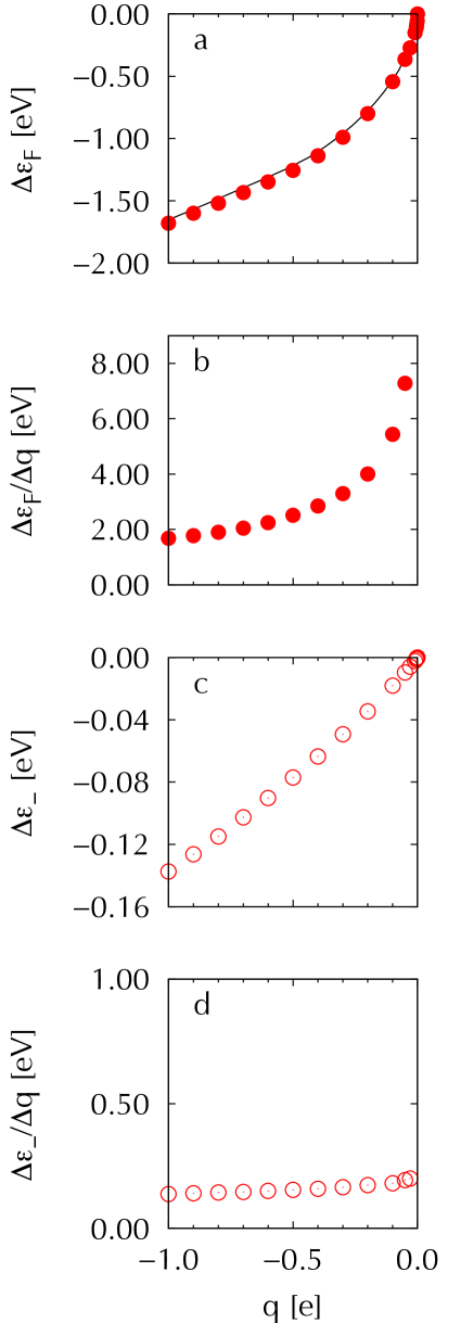
Figure 4: Charge removal in a unit cell of silicon, with $16\times 16\times 16$ $k$-point sampling. Panel a: change in Fermi level position, $\Delta\varepsilon_{F}$, as a function of the removed charge, $\Delta q$. Solid line: change in $\varepsilon_{F}$ expected from the uncharged density of states curve. Panel b: Numerical derivative of the data in panel a, $\Delta\varepsilon_{F}/\Delta q$, as a function of $\Delta q$. Panel c: change in position of valence band maximum, $\Delta\varepsilon_{-}$, as a function of $\Delta q$. Panel d: Numerical derivative of the data in panel c, $\Delta\varepsilon_{-}/\Delta q$, as a function of $\Delta q$.

The above considerations are illustrated numerically in Fig. 4, where the dependence of $\varepsilon_{F}$ on $q$ (a) and its derivative (b) were computed for a primitive unit cell of silicon with a $16\times 16\times 16$ $k$-point sampling scheme. Clearly, and as expected from Eq. (19), the Fermi energy follows closely the integrated density of states of the uncharged system (shown as a solid line). Furthermore, for small $q$ it indeed follows a $q^{2/3}$ law and its derivative diverges.

Fortunately, an equally simple, yet accurate, procedure is to consider instead the valence band maximum (or the conduction band minimum for charge addition), which we denote here as $\varepsilon_{-}$. For $q\to 0$ it too must tend to the correct limit as charge is removed only from the highest occupied state. For finite $q$ it is, of course, incorrect, but as it does not incorporate DOS effects its derivative is not expected to diverge. This is illustrated numerically in Fig. 4 as well, for the same silicon example, where both the weaker dependence of $\varepsilon_{-}$ on $q$ (c - note scale) and the convergence of its derivative for small $q$ (d) is apparent.

In the calculations of Fig. 4, the removal of charge $q$ from a unit cell, sampled by $N$ $k$-points, is in fact equivalent to the removal of the same charge from a reference cell whose volume is $N$ times larger. Using Eq. (15), this means that the limiting value of $\Delta\varepsilon_{-}/\Delta q$ is directly comparable to the non-vanishing unit-cell curvature, $C_{UC}$, rather than to the vanishing reference cell curvature, $C_{RC}$. This is directly verified in Fig. 5, which compares, for silicon, unit-cell curvature values, $C_{UC}$, obtained from increasingly large single $k$-point reference cells (as in Fig. 3) with those obtained from increasingly dense $k$-point sampling of a unit cell. Clearly, the results are indeed equivalent.

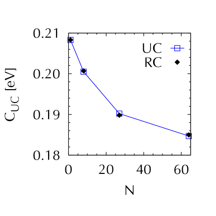
Figure 5: Unit cell curvature, $C_{UC}$, obtained from single $k$-point calculations of a reference cell containing $N$ unit cells (filled diamonds) and from $N$ $k$-point calculations of a single unit cell (hollow squares), as a function of $N$. Lines joining the results of the $N$ $k$-point calculations are a guide to the eye.

Finally, with the above scheme, we efficiently calculate unit-cell curvatures for charge removal and addition in a variety of semiconductors and insulators, obtained in the limit of sufficiently dense $k$-point sampling. The results are summarized in Table 1.

From the results it is clear that for all systems considered the unit cell curvature in LDA is a non zero, material-dependent property. Furthermore, once convergence has been reached it is independent of the density of the $k$-point sampling. This is to be contrasted with the reference cell curvature discussed earlier, which was not only dependent on the reference cell size, but went to zero in the infinite limit for all functionals. As noted in the preceding section, $C_{UC}$ can have both positive and negative values (illustrated by the results in 1), owing to the presence of the neutralizing background.

	Crystal Structure	$C_{UC}\,\left(eV\right)$
		Charge removal	Charge addition
AlAs	Zinc-blende	0.26	-0.65
AlN	Zinc-blende	0.94	-0.92
AlP	Zinc-blende	0.33	-0.66
AlSb	Zinc-blende	0.16	-0.57
C	Diamond	0.58	-0.62
GaP	Zinc-blende	0.36	-0.65
MgO	Rock-salt	1.6	-0.73
Si	Diamond	0.17	-0.54
SiC	Zinc-blende	0.59	-0.64

Table 1: Energy curvature for the unit cell, $C_{UC}$, for charge removal and addition, calculated for various solids.

IV Conclusions

In this article, we have examined the solid-state limit of energy curvature, i.e., of deviations from piecewise-linearity, focusing on (semi-)local functionals. We considered two different limits: finite systems, with volume $\Omega\to\infty$, as well as topologically periodic systems with a reference cell (to which the periodic boundary conditions are applied) of volume $\Omega_{RC}\to\infty$. We found that in all cases piecewise-linearity - albeit possibly with the wrong slope - is obtained in the solid-state limit, even from functionals that grossly disobey it for a finite system. However, using both analytical considerations and practical calculations of representative systems, we found that this limit is reached in very different ways. Therefore, while using the demand of zero curvature for functional construction and evaluation is not, as such, useful in the solid-state limit, its size-dependence does contain useful information.

For large finite systems, we found that curvature scales as $\Omega^{-1/3}$ for three-dimensional systems (e.g., nanocrystals) and as $\frac{2}{L}\ln\left(2e^{-3/4}\frac{L}{a}\right)$, where $L$ is the length and $a$ is the width, for quasi-one-dimensional systems (e.g., molecular chains). This scaling behavior was found to be dominated by electrostatics and traced to the self-interaction term of the highest occupied state.

For large reference cell periodic systems, we found that the curvature $C_{RC}$ scales as $C_{RC}=C_{UC}\Omega_{UC}/\Omega_{RC}$, where $C_{UC}$ and $\Omega_{UC}$ are the unit-cell curvature and volume respectively. $C_{UC}$ (for an approximate functional) is a non-vanishing material-dependent quantity that is independent of the reference cell, and therefore may serve as a new useful measure of functional error in periodic solids, similar to that of the deviation from piecewise linearity used in finite systems. Furthermore, we have been able to calculate this curvature in two ways: either directly from the definition by using increasingly large periodic cells or, more usefully, by considering changes in the band edge position with increasingly dense $k$-point sampling. Last but not least, we rationalized the difference between the periodic and non-periodic case as resulting from the automatic elimination of the spurious self-interaction via the addition of a compensating background charge in periodic system.

We believe that these results should prove useful for further development, evaluation, and application of novel exchange-correlation functionals suitable for the solid-state.

V Acknowledgments

We thank Eli Kraisler, Sivan Refaely-Abramson (Weizmann Institute), and Stephan Kümmel (Universität Bayreuth) for useful discussions. Work at the Weizmann Institute was supported by the European Research Council. Work at the Hebrew University of Jerusalem was supported by the Israel Science Foundation Grant No. 1219-12. Some of the computations (VV) were performed at the Leibniz Supercomputing Centre of the Bavarian Academy of Sciences and the Humanities.

References

- (1) P. Hohenberg and W. Kohn, Phys. Rev. 136, B864 (1964)
- (2) W. Kohn and L. J. Sham, Phys. Rev. 140, A1133 (1965)
- (3) M. Levy, Phys. Rev. A 26, 1200 (1982)
- (4) E. H. Lieb, Int. J. Quantum Chem. 24, 243 (1983)
- (5) For spin unpolarized (polarized) KS systems the value of the occupation number is equal to if , equal to if and if , where , the highest occupied eigenvalue, is determined such that is equal to the total number of electrons . The lowest eigenvalue for which is referred to as .
- (6) J. P. Perdew and S. Kurth, A Primer in Density Functional Theory (Springer, 2003)
- (7) J. P. Perdew, R. G. Parr, M. Levy, and J. L. Balduz, Phys. Rev. Lett. 49, 1691 (1982)
- (8) J. Janak, Phys. Rev. B 18, 7165 (1978)
- (9) M. Levy, J. P. Perdew, and V. Sahni, Phys. Rev. A 30, 2745 (1984)
- (10) C.-O. Almbladh and U. von Barth, Phys. Rev. B 31, 3231 (1985)
- (11) J. P. Perdew and M. Levy, Phys. Rev. B 56, 16021 (1997)
- (12) A. D. Becke, J. Chem. Phys. 98, 1372 (1993)
- (13) P. Mori-Sánchez, A. J. Cohen, and W. T. Yang, J. Chem. Phys. 125, 201102 (2006)
- (14) A. Ruzsinszky, J. P. Perdew, G. I. Csonka, O. A. Vydrov, and G. E. Scuseria, J. Chem. Phys. 126, 104102 (2007)
- (15) O. A. Vydrov, G. E. Scuseria, and J. P. Perdew, J. Chem. Phys. 126, 154109 (2007)
- (16) P. Mori-Sánchez, A. J. Cohen, and W. Yang, Phys. Rev. Lett. 100, 146401 (2008), http://prl.aps.org/abstract/PRL/v100/i14/e146401
- (17) A. J. Cohen, P. Mori-Sánchez, and W. T. Yang, Science 321, 792 (2008)
- (18) A. J. Cohen, P. Mori-Sánchez, and W. T. Yang, Phys. Rev. B 77, 115123 (2008)
- (19) R. Haunschild, T. M. Henderson, C. A. Jiménez-Hoyos, and G. E. Scuseria, J. Chem. Phys. 133, 134116 (2010)
- (20) M. Srebro and J. Autschbach, J. Phys. Chem. Lett. 3, 576 (2012)
- (21) J. D. Gledhill, M. J. Peach, and D. J. Tozer, J. Chem. Theory Comput. 9, 4414 (2013), http://pubs.acs.org/doi/abs/10.1021/ct400592a
- (22) A. J. Cohen and P. Mori-Sánchez, J. Chem. Phys. 140, 044110 (2014), http://scitation.aip.org/content/aip/journal/jcp/140/4/10.1063/1.4858461
- (23) D. J. Tozer, Phys. Rev. A 58, 3524 (1998)
- (24) M. J. Allen and D. J. Tozer, Mol. Phys. 100, 433 (2002)
- (25) J. P. Perdew and M. Levy, Phys. Rev. Lett. 51, 1884 (1983)
- (26) L. J. Sham and M. Schluter, Phys. Rev. Lett. 51, 1888 (1983)
- (27) J. P. Perdew and M. Levy, Phys. Rev. B 31, 6264 (1985)
- (28) E. Sagvolden and J. P. Perdew, Phys. Rev. A 77, 012517 (2008)
- (29) Where the interacting-electron system is mapped into a partially interacting electron gas that is still represented by a single Slater determinant (Seidl1996, ).
- (30) A. Seidl, A. Görling, P. Vogl, J. A. Majewski, and M. Levy, Phys. Rev. B 53, 3764 (1996)
- (31) S. Kümmel and L. Kronik, Rev. Mod. Phys. 80, 3 (2008)
- (32) W. Yang, A. J. Cohen, and P. Mori-Sánchez, J. Chem. Phys. 136, 204111 (2012)
- (33) H. R. Eisenberg and R. Baer, Phys. Chem. Chem. Phys. 11, 4674 (2009)
- (34) T. Stein, H. Eisenberg, L. Kronik, and R. Baer, Phys. Rev. Lett. 105, 266802 (2010)
- (35) L. Kronik, T. Stein, S. Refaely-Abramson, and R. Baer, J. Chem. Theory Comput. 8, 1515 (2012)
- (36) T. Stein, J. Autschbach, N. Govind, L. Kronik, and R. Baer, J. Phys. Chem. Lett. 3, 3740 (2012)
- (37) M. Cococcioni and S. de Gironcoli, Phys. Rev. B 71, 035105 (2005)
- (38) S. Lany and A. Zunger, Phys. Rev. B 80, 085202 (2009)
- (39) I. Dabo, A. Ferretti, N. Poilvert, Y. L. Li, N. Marzari, and M. Cococcioni, Phys. Rev. B 82, 115121 (2010)
- (40) J. D. Chai and P. T. Chen, Phys. Rev. Lett. 110, 033002 (2013)
- (41) A. Ferretti, I. Dabo, M. Cococcioni, and N. Marzari, Phys. Rev. B 89, 195134 (2014)
- (42) E. Kraisler and L. Kronik, Phys. Rev. Lett. 110, 126403 (2013)
- (43) E. Kraisler and L. Kronik, J. Chem. Phys. 140, 18A540 (2014), http://scitation.aip.org/content/aip/journal/jcp/140/18/10.1063/1.4871462
- (44) M. Kuisma, J. Ojanen, J. Enkovaara, and T. T. Rantala, Phys. Rev. B 82, 115106 (2010)
- (45) R. Armiento and S. Kümmel, Phys. Rev. Lett. 111, 36402 (2013)
- (46) N. Sai, P. F. Barbara, and K. Leung, Phys. Rev. Lett. 106, 226403 (2011)
- (47) V. Atalla, M. Yoon, F. Caruso, P. Rinke, and M. Scheffler, Phys. Rev. B 88, 165122 (2013)
- (48) R. Baer, E. Livshits, and U. Salzner, Annu. Rev. Phys. Chem. 61, 85 (2010)
- (49) J. Autschbach and M. Srebro, Acc. Chem. Res.(2014)
- (50) S. Öğüt, J. R. Chelikowsky, and S. G. Louie, Phys. Rev. Lett. 79, 1770 (1997)
- (51) R. W. Godby and I. D. White, Phys. Rev. Lett. 80, 3161 (1998)
- (52) U. Salzner, J. Phys. Chem. A 114, 10997 (2010)
- (53) G. Onida, L. Reining, and A. Rubio, Rev. Mod. Phys. 74, 601 (2002)
- (54) A. F. Izmaylov and G. E. Scuseria, J. Chem. Phys. 129, 034101 (2008)
- (55) In this paper all systems are treated strictly in the closed shell spin-unpolarized ensemble, so any removal or addition of small amounts of electronic charge preserves the unpolarized spin nature of the system.
- (56) Obviously the lowest-unoccupied eigenstate becomes the highest-occupied one upon charge addition.
- (57) J. Hellman, Einführung in die Quantenchemie (Deuticke, Leipzig, 1937)
- (58) R. P. Feynman, Phys. Rev. 56, 340 (1939)
- (59) U. Salzner and R. Baer, J. Chem. Phys. 131, 231101 (2009)
- (60) M. Petersilka, U. J. Gossmann, and E. K. U. Gross, Phys. Rev. Lett. 76, 1212 (1996)
- (61) D. Finocchiaro, M. Pellegrini, and P. Bientinesi, J. Comput. Phys. 146, 707 (1998)
- (62) R. Godby, M. Schlüter, and L. Sham, Phys. Rev. B 36, 6497 (1987), http://journals.aps.org/prb/abstract/10.1103/PhysRevB.36.6497
- (63) J. R. Chelikowsky and M. L. Cohen, “Ab initio pseudopotentials for semiconductors,” in Handbook on Semiconductors, Vol. 1, edited by T. S. Moss and P. T. Landsberg (Elsevier, Amsterdam, the Netherlands, 1992) p. 59
- (64) M. Valiev, E. J. Bylaska, N. Govind, K. Kowalski, T. P. Straatsma, H. J. J. Van Dam, D. Wang, J. Nieplocha, E. Apra, T. L. Windus, and W. A. de Jong, Comput. Phys. Commun. 181, 1477 (2010)
- (65) D. V. Melnikov and J. R. Chelikowsky, Phys. Rev. B 69, 113305 (2004)
- (66) O. Ciftja, Physica B 407, 2803 (2012)
- (67) L. Segev, A. Salomon, A. Natan, D. Cahen, L. Kronik, F. Amy, C. K. Chan, and A. Kahn, Phys. Rev. B 74, 165323 (2006), http://journals.aps.org/prb/abstract/10.1103/PhysRevB.74.165323
- (68) N. W. Ashcroft and N. D. Mermin, Solid State Physics (Holt, Rinehart and Winston, New York, 1976) (2005)
- (69) Alternatively, the bulk limit can be approached using the concept of -point sampling of the unit cell. Pickett1989 For now, we do not pursue this alternative, but we discuss it extensively below
- (70) J. Ihm, A. Zunger, and M. L. Cohen, J. Phys.: Condens. Matter 12, 4409 (1979), http://iopscience.iop.org/0022-3719/12/21/009
- (71) S. Sharma, J. Dewhurst, N. Lathiotakis, and E. Gross, Phys. Rev. B 78, 201103 (2008), http://prb.aps.org/abstract/PRB/v78/i20/e201103
- (72) The same dependence on can be obtained by considering the curvature directly as the second derivative of the energy, i.e., , because and are both extensive quantities and therefore proportional to .
- (73) We performed non-spin-polarized calculations using norm-conserving pseudopotentials within the Quantum-ESPRESSO (QE-2009, ) and ABINIT (gonze2002first, ; gonze2005brief, ) packages, which use a planewave basis with periodic boundary conditions. All results were converged for plane-wave kinetic energy cut-off.
- (74) LDA erroneously predicts bulk germanium to be semi-metallic (see, e.g., J. Heyd, J. E. Peralta, G. E. Scuseria, and R. L. Martin, J. Chem. Phys. 123, 174101 (2005)). Therefore, germanium is omitted from Fig. 3
- (75) I. Solovyev, P. Dederichs, and V. Anisimov, Phys. Rev. B 50, 16861 (1994), http://journals.aps.org/prb/abstract/10.1103/PhysRevB.50.16861
- (76) W. E. Pickett, Computer Physics Reports 9, 115 (1989)
- (77) C. Kittel, Introduction to solid state physics, 3rd ed. (Wiley, New York,, 1966) p. 648 p.
- (78) P. Giannozzi, S. Baroni, N. Bonini, M. Calandra, R. Car, C. Cavazzoni, D. Ceresoli, G. L. Chiarotti, M. Cococcioni, I. Dabo, A. Dal Corso, S. de Gironcoli, S. Fabris, G. Fratesi, R. Gebauer, U. Gerstmann, C. Gougoussis, A. Kokalj, M. Lazzeri, L. Martin-Samos, N. Marzari, F. Mauri, R. Mazzarello, S. Paolini, A. Pasquarello, L. Paulatto, C. Sbraccia, S. Scandolo, G. Sclauzero, A. P. Seitsonen, A. Smogunov, P. Umari, and R. M. Wentzcovitch, J. Phys.: Condens. Matter 21, 395502 (19pp) (2009), http://www.quantum-espresso.org
- (79) X. Gonze, J.-M. Beuken, R. Caracas, F. Detraux, M. Fuchs, G.-M. Rignanese, L. Sindic, M. Verstraete, G. Zerah, F. Jollet, et al., Computational Materials Science 25, 478 (2002)
- (80) X. Gonze, G.-M. Rignanese, M. Verstraete, J.-M. Beuken, Y. Pouillon, R. Caracas, F. Jollet, M. Torrent, G. Zerah, M. Mikami, et al., Z. Kristallogr. 220, 558 (2005)