The Pierre Auger Collaboration
Depth of Maximum of Air-Shower Profiles at the Pierre Auger Observatory: Measurements at Energies above eV
Abstract
We report a study of the distributions of the depth of maximum, , of extensive air-shower profiles with energies above eV as observed with the fluorescence telescopes of the Pierre Auger Observatory. The analysis method for selecting a data sample with minimal sampling bias is described in detail as well as the experimental cross-checks and systematic uncertainties. Furthermore, we discuss the detector acceptance and the resolution of the measurement and provide parameterizations thereof as a function of energy. The energy dependence of the mean and standard deviation of the -distributions are compared to air-shower simulations for different nuclear primaries and interpreted in terms of the mean and variance of the logarithmic mass distribution at the top of the atmosphere.
I Introduction
The mass composition of ultra-high energy cosmic rays is one of the key observables in studies of the origin of these rare particles. At low and intermediate energies between and eV, precise data on the composition are needed to investigate a potential transition from galactic to extragalactic sources of the cosmic-ray flux (see, e.g., Linsley63 ; Hillas:2005cs ; Allard:2005cx ; Aloisio:2006wv ). Furthermore, the evolution of the composition towards eV will help to understand the nature of the steepening of the flux of cosmic rays observed at around Abbasi:2007sv ; Abraham:2008ru ; AbuZayyad:2012ru . This flux suppression might either be caused by energy losses of extragalactic particles due to interactions with photons (cosmic microwave background in case of protons or extragalactic background light in case of heavy nuclei) greisen-66 ; Zatsepin:1966jv , or it might signify the maximum of attainable energy in astrophysical accelerators, resulting in a rigidity-dependent change of the composition (see, e.g., peters61 ; Allard:2008gj ; Aloisio:2009sj ; Hooper:2009fd ; Fang:2013cba ).
Due to the low intensity of cosmic rays at the highest energies, the primary mass cannot be measured directly but is inferred from the properties of the particle cascade initiated by a primary cosmic ray interacting with nuclei of the upper atmosphere. These extensive air showers can be observed with ground-based detectors over large areas. The mass and energy of the primary particles can be inferred from the properties of the longitudinal development of the cascade and the particle densities at the ground after making assumptions about the characteristics of high-energy interactions (see, e.g., Kampert:2012mx for a recent review).
The energy deposited in the atmosphere by the secondary air-shower particles is dominated by electron and positron contributions. The development of the corresponding electromagnetic cascade Greisen:1960wc is best described as a function of traversed air mass, usually referred to as the slant depth . It is obtained by integrating the density of air along the direction of arrival of the air shower through the curved atmosphere,
| (1) |
where is the density of air at a point with longitudinal coordinate along the shower axis.
The depth at which the energy deposit reaches its maximum is the focus of this article. The depth of shower maximum, , is proportional to the logarithm of the mass of the primary particle. However, due to fluctuations of the properties of the first few hadronic interactions in the cascade, the primary mass cannot be measured on an event-by-event basis but must be inferred statistically from the distribution of shower maxima of an ensemble of air showers. Given that nuclei of mass produce a distribution , the overall distribution is composed of the superposition
| (2) |
where the fraction of primary particle of type is given by . The first two moments of , i.e., its mean and variance, and respectively, have been extensively studied in the literature elong1 ; elong2 ; elong3 ; LinsleyXmax1983 ; LinsleyXmax1985 ; semisuper ; Matthews:2005sd . They are to a good approximation linearly related to the first two moments of the distribution of the logarithm of the primary mass , which is given by the superposition
| (3) |
where is the Dirac delta function.
The exact shape of as well as the coefficients that relate the moments of to the ones of depend on the details of hadronic interactions in air showers (see, e.g., Ulrich:2010rg ; Parsons:2011ad ; Engel:2011zzb ). On the one hand, this introduces considerable uncertainties in the interpretation of the distributions in terms of primary mass, since the modeling of these interactions relies on extrapolations of accelerator measurements to cosmic-ray energies. On the other hand, it implies that the distributions can be used to study properties of hadronic interactions at energies much larger than currently available in laboratory experiments. A recent example of such a study is the measurement of the proton-air cross section at using the upper tail of the distribution Abreu:2012wt .
Experimentally, the longitudinal profile of the energy deposit of an air shower in the atmosphere (and thus ) can be determined by observing the fluorescence light emitted by nitrogen molecules excited by the charged particles of the shower. The amount of fluorescence light is proportional to the energy deposit Belz:2006 ; Ave:2008zza and can be detected by optical telescopes. The instrument used in this work is described in Sec. II and the reconstruction algorithms leading to an estimate of are laid out in Sec. III.
Previous measurements of with the fluorescence technique have concentrated on the determination of the mean and standard deviation of the distribution flysEyeXmax1990 ; Abbasi:2004nz ; Abbasi:2009nf ; Abraham:2010yv . Whereas with these two moments the overall features of primary cosmic-ray composition can be studied, and composition fractions in a three-component model can even be derived, only the distribution contains the full information on composition and hadronic interactions that can be obtained from measurements of .
In this paper, we provide for the first time the measured distributions together with the necessary information to account for distortions induced by the measurement process. The relation between the true and observed distribution is
| (4) |
i.e., the true distribution is deformed by the detection efficiency and smeared by the detector resolution that relates the true to the reconstructed one, . For an ideal detector, is constant and is close to a delta function. In Sec. IV, we describe the fiducial cuts applied to the data that guarantee a constant efficiency over a wide range of and the quality cuts that assure a good resolution. Parameterization of and are given in Sec. V and VI.
Given , and it is possible to invert Eq. (4) to obtain the true distribution . However, since is obtained from a limited number of events, its statistical uncertainties propagate into large uncertainties and negative correlations of the deconvoluted estimator of the true distribution, . In practice, methods which reduce the uncertainties of by applying additional constraints to the solution exist (see, e.g., Cowan:2002in ), but these constraints introduce biases that are difficult to quantify. Therefore we choose to publish together with parameterizations of and . In Sec. VII it is demonstrated how to derive and from , and . The systematic uncertainties in the measurement of are discussed in Sec. VIII and validated in Sec. IX. In Sec. X the measured distributions will be shown in bins of energy reaching from to together with a discussion of their first two moments.
II The Pierre Auger Observatory
In this paper we present data from the Pierre Auger Observatory Abraham:2004dt . It is located in the province of Mendoza, Argentina, and consists of a Surface-Detector array (SD) Allekotte:2007sf and a Fluorescence Detector (FD) Abraham:2009pm . The SD is equipped with over 1600 water-Cherenkov detectors arranged in a triangular grid with a 1500 m spacing, detecting photons and charged particles at ground level. This 3000 km2 array is overlooked by 24 fluorescence telescopes grouped in units of 6 at four locations on its periphery. Each telescope collects the light of air showers over an aperture of 3.8 m2. The light is focused on a photomultiplier (PMT) camera with a 13 m2 spherical mirror. Corrector lenses at the aperture minimize spherical aberrations of the shower image on the camera. Each camera is equipped with 440 PMT pixels, whose field of view is approximately 1.5∘. One camera covers 30∘ in azimuth and elevations range from to 30∘ above the horizon. The FD allows detection of the ultraviolet fluorescence light induced by the energy deposit of charged particles in the atmosphere and thus measures the longitudinal development of air showers. Whereas the SD has a duty cycle near 100%, the FD operates only during dark nights and under favorable meteorological conditions leading to a reduced duty cycle of about 13%.
Recent enhancements of the Observatory include a sub-array of surface detector stations with a spacing of 750 m and three additional fluorescence telescopes with a field of view from to co-located at one of the “standard” FD sites Amiga ; HEAT . These instruments are not used in this work, but they will allow us to extend the analysis presented here to lower energies () heatPaper .
In addition to the FD and SD, important prerequisites for a precise measurement of the energy and of showers are devices for the calibration of the instruments and the monitoring of the atmosphere.
The calibration of the fluorescence telescopes in terms of photons at aperture per ADC count in the PMTs is achieved by approximately yearly absolute calibrations with a Lambertian light source of known intensity and nightly relative calibrations with light-emitting diodes illuminating the FD cameras Brack:2004af ; Bauleo:2008iz ; Brack:2013bta . The molecular properties of the atmosphere at the time of data taking are obtained as the 3-hourly data tables provided by the Global Data Assimilation System (GDAS) gdas , which have been extensively cross-checked with radio soundings on site Abreu:2012zg . The aerosol content of the atmosphere during data taking is continuously monitored Abraham:2010pf . For this purpose, the vertical aerosol optical depth (VAOD) is measured on an hourly basis using laser shots provided by two central laser facilities (CLFs) Arqueros:2005yn ; Abreu:2013qtw and cross-checked by lidars BenZvi:2006xb operated at each FD site. Finally, clouds are detected via observations in the infrared by cameras installed at each FD site Chirinos:ICRC2013 and data from the Geostationary Operational Environmental Satellites (GOES) goes ; Abreu:2013qfa
III Event Reconstruction
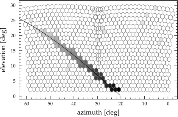
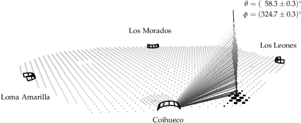
The reconstruction of the data is performed within the offline framework of the Pierre Auger Observatory Argiro:2007qg . Firstly, all PMT pixels belonging to the shower image on the camera are identified using a Hough-transformation and subsequently fitted to reconstruct the plane spanned by the axis of the incoming shower and the telescope position. Within this plane a three-dimensional reconstruction of the shower-arrival direction is achieved by determining the geometry from the arrival times of the shower light as a function of viewing angle Porter:1970et and from the time of arrival of the shower front at ground level as measured by the surface-detector station closest to the shower axis. This leads to a hybrid estimate of the shower geometry with a precision of typically 0.6∘ for the arrival direction of the primary cosmic ray Sommers:1995dm ; Dawson:1996ci ; angular . An example of the image of a shower in an FD camera is shown in Fig. 1a and the reconstructed geometry is shown in Fig. 1b.
The detected signals in the PMTs of the telescope cameras as a function of time are then converted to a time-trace of light at the aperture using the calibration of the absolute and relative response of the optical system. At each time , the signals of all PMTs with pointing directions within an opening angle with respect to the corresponding direction towards the shower are summed up. is determined on an event-by-event basis by maximizing the ratio of the collected signal to the accumulated noise induced by background light from the night sky. The average of the events used in this analysis is 1.3∘, reaching up to 4∘ for showers detected close to the telescope. The amount of light outside of due to the finite width of the shower image Gora:2005sq ; Giller:2009zz and the point spread function of the optical system augerPSF1 ; augerPSF2 is corrected for in later stages of the reconstruction and multiply-scattered light within is also accounted for Roberts:2005xv ; Pekala:2009fe ; Giller:2012tt .
With the help of the reconstructed geometry, every time bin is projected to a piece of path length on the shower axis centered at height and slant depth . The latter is inferred by integrating the atmospheric density through a curved atmosphere. Given the distance to the shower, the light at the aperture can be projected to the shower axis to estimate the light emitted by the air-shower particles along , taking into account the attenuation of light due to Rayleigh scattering on air and Mie scattering on aerosols.
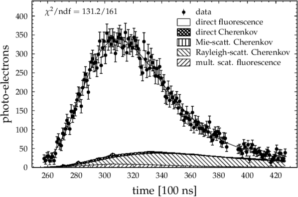
The light from the shower is composed of fluorescence and Cherenkov photons. The production yield of the former is proportional to the energy deposited by the shower particles within the volume under study, and the latter depends on the number of charged particles above the energy threshold for Cherenkov emission. Due to the universality of the energy spectra of electrons and positrons in air showers cher:giller ; cher:hillaslongi ; cher:nerling ; Lafebre:2009en , the energy deposit and the number of particles are proportional, and therefore an exact solution for the reconstruction of the longitudinal profile of either of these quantities exists Unger:2008uq . An example of a profile of the reconstructed energy deposit can be seen in Fig. 1d and the contributions of the different light components to the detected signal are shown in Fig. 1c. The Cherenkov light production is calculated following cher:nerling and for the fluorescence-light emission along the shower we use the precise laboratory measurements of the fluorescence yield from Ave:2007xh ; Ave:2012ifa .
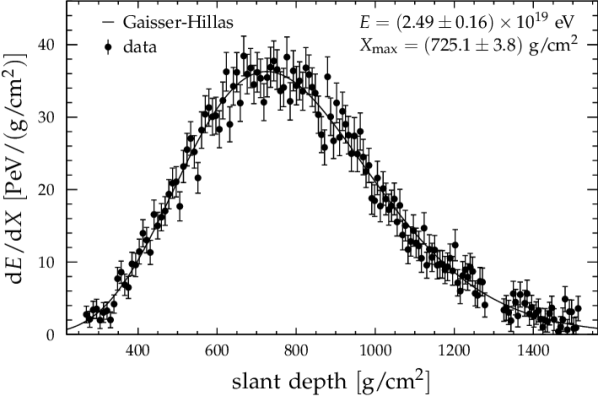
In the final step of the reconstruction, the shower maximum and total energy are obtained from a log-likelihood fit of the number of photo-electrons detected in the PMTs using the Gaisser-Hillas function ghfunc , , as a functional description of the dependence of the energy deposit on slant depth,
| (5) |
The two shape parameters and are constrained to their average values to allow for a gradual transition from a two- to a four-parameter fit depending on the amount of slant depth observed along the track and the number of detected photons from the respective event, cf. Unger:2008uq . The constraints are set to the average values found in the ensemble of events for which an unconstrained fit with four-parameters is possible. They are given by and , and the observed standard deviations of these sample means are 172 and 13 , respectively. An example of a Gaisser-Hillas function that has been obtained by the log-likelihood fit to the detected photo-electrons in Fig. 1c is shown in Fig. 1d.
The calorimetric energy of the shower is obtained by the integration of and the total energy is derived after correcting for the “invisible” energy, carried away by neutrinos and muons. This correction has been estimated from hybrid data eInv and is of the order of 10 to 15% in the energy range relevant for this study.
IV Data Selection
The analysis presented in this paper is based on data collected by the Pierre Auger Observatory from the 1st of December 2004 to the 31st of December 2012 with the four standard FD sites. The initial data set consists of about shower candidates that met the requirements of the four-stage trigger system of the data acquisition. Since only very loose criteria need to be fulfilled at a trigger level (basically a localized pattern of four pixels detecting a pulse in a consecutive time order), a further selection of the events is applied off-line as shown in Tab. 1 and explained in more detail in the following section.
| cut | events | [%] |
| pre-selection: | ||
| air-shower candidates | 2573713 | - |
| hardware status | 1920584 | 74.6 |
| aerosols | 1569645 | 81.7 |
| hybrid geometry | 564324 | 35.9 |
| profile reconstruction | 539960 | 95.6 |
| clouds | 432312 | 80.1 |
| 111194 | 25.7 | |
| quality and fiducial selection: | ||
| 105749 | 95.1 | |
| observed | 73361 | 69.4 |
| quality cuts | 58305 | 79.5 |
| fiducial field of view | 21125 | 36.2 |
| profile cuts | 19947 | 94.4 |
IV.1 Pre-Selection
In the first step, a pre-selection is applied to the air-shower candidates resulting in a sample with minimum quality requirements suitable for subsequent physics analysis.
Only time periods with good data-taking conditions are selected using information from databases and results from off-line quality-assurance analyses. Concerning the status of the FD telescopes, a high-quality calibration of the gains of the PMTs of the FD cameras is required and runs with an uncertain relative timing with respect to the surface detector are rejected using information from the electronic logbook and the slow-control database. Furthermore, data from one telescope with misaligned optics are not used prior to the date of realignment. In total, this conservative selection based on the hardware status removes about 25% of the initial FD triggers. Additional database cuts are applied to assure a reliable correction of the attenuation of shower light due to aerosols: events are only accepted if a measurement of the aerosol content of the atmosphere is available within one hour of the time of data taking. Periods with poor viewing conditions are rejected by requiring that the measured VAOD, integrated from the ground to 3 km, is smaller than 0.1. These two requirements reduce the event sample by 18%.
For an analysis of the shower maximum as a function of energy, a full shower reconstruction of the events is needed. The requirement of a reconstructed hybrid geometry is fulfilled for about 36% of the events that survived the cuts on hardware status and atmospheric conditions. This relatively low efficiency is partially due to meteorological events like sheet lightning at the horizon that pass the FD trigger criteria but are later discarded in the event reconstruction. Moreover, below the probability for at least one triggered station in the standard 1.5 km grid of the surface detector drops quickly Abreu:2010aa . Therefore, a fit of the geometry using hybrid information is not possible for the majority of the showers of low energy that trigger the data-acquisition system of the FD.
A full reconstruction of the longitudinal profile, including energy and , is possible for most of the events with a hybrid geometry. Less than 5% of the events cannot be reconstructed, because too few profile points are available and/or their statistical precision is not sufficient. This occurs for either showers that are far away from the telescopes and close to the trigger threshold or for geometries pointing towards the telescope for which the trace of light at the camera is highly time-compressed.
A possible reflection or shadowing of the light from the shower by clouds is excluded by combining information from the two laser facilities, the lidars and the cloud monitoring devices described in Sec. II. Events are accepted if no cloud is detected along the direction to the shower in either the telescope projection (cloud camera) or ground-level projection (GOES). Furthermore, events are accepted if the base-height of the cloud layer as measured by both the lidars and lasers is above the geometrical field of view or 400 above the fiducial field of view. The latter variable is explained in the next section. When none of these requirements are met, events are rejected if either the cloud camera or GOES indicates the presence of clouds in their respective projections. When no data from these monitors are available, the event is accepted if during the data-taking the average cloud fraction as reported by lidars is below 25%, otherwise the event is not used. In that way, about 80% of the events are labeled as cloud-free.
In the final step of the pre-selection, we apply the lower energy threshold of this analysis, , which reduces the data set by another 75% to events available for further analysis.
IV.2 Quality and Fiducial Selection
After the pre-selection described above, the remaining part of the analysis is focused on defining a subset of the data for which the distortion of the distribution is minimal, i.e., to achieve a good resolution via quality cuts and a uniform acceptance to showers in a large range of possible values.
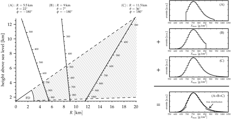
Before giving the technical details of the selection below, it is instructive to discuss first some general considerations about the sampling of the distribution with fluorescence detectors. The position of the shower maximum can only be determined reliably if the point itself is observed within the field of view of the telescopes. The inference of from only the rising or falling edge of the profile would introduce a large dependency of the results on the functional form of the profile (e.g., Gaisser-Hillas function) and the constraints on the shape parameters. The standard telescopes of the Pierre Auger Observatory are used to observe shower profiles within elevation angles from 1.5∘ to 30∘. This geometrical field of view sets an upper and lower limit on the range of detectable shower maxima for a given arrival direction and core location, as illustrated in Fig. 2 for three example geometries. Nearby showers with an axis pointing away from the detector have the smallest acceptance for shallow showers (geometry (A)), whereas vertical showers cannot be used to sample the deep tail of the distribution for depths larger the vertical depth of the ground level, which is about 860 for the Malargüe site (geometry (B)). Ideal conditions for measuring a wide range of are realized by a geometry that intercepts the upper field of view at low slant depths and by inclined arrival directions, for which the slant depth at the ground is large (geometry (C)). The true distribution considered for all three cases is identical and indicated as a solid line. If the frequencies of shower maxima detected with all occurring geometries are collected in one histogram, then the resulting observed distribution will be under-sampled in the tails at small and large depths, as illustrated by the (A+B+C)-distribution in the lower right of Fig. 2.
In addition to these simple geometrical constraints, the range of viewable depths is limited by the following two factors. Firstly, showers cannot be observed to arbitrary distances, but for a given energy the maximum viewing distance depends on background light from the night sky (as a function of elevation) and the transmissivity of the atmosphere. Therefore, even if shower (C) has a large geometrical field of view, in general will not be detectable at all depths along the shower axis. Secondly, if quality cuts are applied to the data, the available range in depth depends on the selection efficiency and therefore the corresponding effective field of view will usually be a complicated function of energy, elevation and distance to the shower maximum.
In this work, we follow a data-driven approach to minimize the deformation of the distributions caused by the effective field of view boundaries. As will be shown in the following, a fiducial selection can be applied to the data to select geometries preferentially with a large accessible field of view as in the case of the example geometry (C) resulting in an acceptance that is constant over a wide range of values. The different steps of the quality and fiducial selection are explained in the following.
Hybrid Probability
After the pre-selection, only events with at least one triggered station of the SD remain in the data set. The maximum allowed distance of the nearest station to the reconstructed core is 1.5 km. For low energies and large zenith angles, the array is not fully efficient at these distances. To avoid a possible mass-composition bias due to the different trigger probabilities for proton- and iron-induced showers, events are only accepted if the average expected SD trigger probability is larger than 95%. The probability is estimated for each event given its energy, core location and zenith angle (cf. Abreu:2011zzd ). This cut removes about 5% of events, mainly at low energies.
observed
It is required that the obtained is within the observed profile range. Events where only the rising and/or falling edge of the profile has been observed are discarded, since in such cases the position of cannot be reliably estimated. As can be seen in Tab. 1, about 30% of the events from the tails of the distribution are lost due to the limited field of view of the FD telescopes.
Quality cuts
Faint showers with a poor resolution are rejected based on the expected precision of the measurement, , which is calculated in a semi-analytic approach by expanding the Gaisser-Hillas function around and then using this linearized version to propagate the statistical uncertainties of the number of photo-electrons at the PMT to an uncertainty of . Only showers with are accepted. Moreover, geometries for which the shower light is expected to be observed at small angles with respect to the shower axis are rejected. Such events exhibit a large contribution of direct Cherenkov light that falls off exponentially with the observation angle. Therefore, even small uncertainties in the event geometry can change the reconstructed profile by a large amount. We studied the behavior of as a function of the minimum observation angle, , and found systematic deviations below , which is therefore used as a lower limit on the allowed viewing angle. About 80% of the events fulfill these quality criteria.
Fiducial Field of View
The aim of this selection is to minimize the influence of the effective field of view on the distribution by selecting only type (C) geometries (cf. Fig. 2).
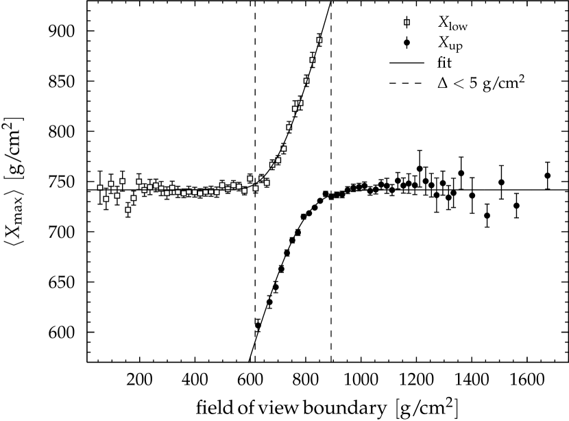
The quality variables and are calculated for different values in steps of 10 along the shower axis within the geometrical field-of-view boundaries. In that way, the effective slant-depth range for high-quality showers can be exactly defined and it is given by the interval in slant depth for which both and . The shower is accepted if this interval is sufficiently large to accommodate the bulk of the distribution. The true distribution is unfortunately not known at this stage of the analysis and therefore we study the differential behavior of on the lower and upper field-of-view boundary, and , for different energy intervals using data. An example is shown in Fig. 3. Once the field of view starts truncating the distribution, the observed deviates from its asymptotically unbiased value. We set the fiducial field-of-view boundaries at the values of and where a deviation of occurs to ensure that the overall sampling bias on is smaller than this value. The energy dependence of these boundaries is then parameterized as
| (6) |
with parameters and for the upper and lower boundary in slant depth, respectively. and are given in units of and is in eV. The requirement that and removes about 64% of all the remaining events.
Profile Quality
In the last step of the selection, three more requirements on the quality of the profiles are applied. Firstly, events with gaps in the profile that are longer than 20% of its total observed length are excluded. Such gaps can occur for showers crossing several cameras, since the light in each camera is integrated only within the PMTs that are more than away from the camera border (see, e.g., the gap at around 1300 in the profile shown in Fig.1d). Secondly, residual cloud contamination and horizontal non-uniformities of the aerosols may cause distortions of the profile which can be identified with the goodness of the Gaisser-Hillas fit. We apply a standard-normal transformation to the of the profile fit, , and reject showers in the non-Gaussian tail at . Finally, a minimum observed track length of is required. These cuts are not taken into account in the calculation of the effective view, but since the selection efficiency is better than 94%, the procedure explained in the last paragraph still yields a good approximation of the field-of-view boundaries.
In total, the quality and fiducial selection has an efficiency of 18%. This number is dominated by low-energy showers, where the profiles are faint and only a small phase space in distance and arrival direction provides a large effective field of view. Nevertheless, as shown in Sec. IX.1, the efficiency of the quality and fiducial selection reaches close to 50% at high energies.
IV.3 Final Data Set
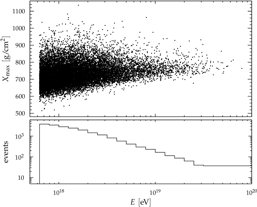
After the application of all selection cuts, 19947 events from the four standard FD sites remain. Air showers that have been observed and selected at more than one FD site are combined by calculating the weighted average of and energy. This leads to 19759 independent air-shower events used for this analysis. Their and energy values are shown as a scatter plot in Fig. 4.
V Acceptance
Even following the event selection described above, the probability to detect and select an air shower is not uniform for arbitrary values of . The corresponding acceptance needs to be evaluated to correct for residual distortions of the distribution. For this purpose we use a detailed, time-dependent simulation Abreu:2010aa of the atmosphere, the fluorescence and surface detector. The simulated events are reconstructed with the same algorithm as the data and the same selection criteria are applied. The acceptance is calculated from the ratio of selected to generated events.
The shape of the longitudinal energy-deposit profiles of air showers at ultra-high energies is, to a good approximation, universal, i.e., it does not depend on the primary-particle type or details of the first interaction Andringa:2011zz . Therefore, after marginalizing over the distances to the detector and the arrival directions of the events, the acceptance depends only on and the calorimetric energy, but not on the primary mass or hadronic interaction model. For practical reasons, and since the calorimetric energies of different primaries with the same total energy are predicted to be within Pierog:2013qdx , we studied the acceptance as a function of total energy and .
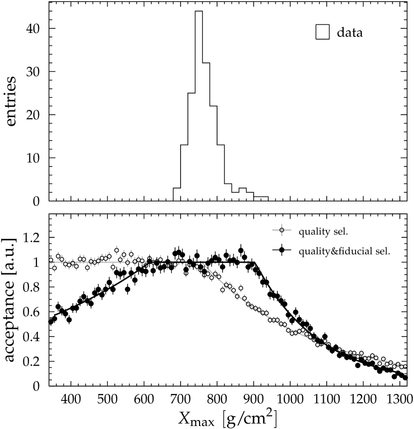
In the lower panel of Fig. 5 an example of the acceptance with and without fiducial field-of-view cuts is shown. Since for the purpose of the measurement of the distribution only the shape of the acceptance is important, the curves have been normalized to give a maximum acceptance of 1. For comparison, the distribution of after the full selection is shown in the upper panel of the figure. As can be seen, the acceptance after application of fiducial cuts is constant over most of the range covered by the selected events. The acceptance without fiducial selection exhibits a constant part too, but it does not match the range of measured events well because it starts to depart from unity already at around the mode of the measured distribution.
Numerically, the acceptance can be parameterized by an exponentially-rising part, a central constant part and an exponentially-falling part,
| (7) |
with energy-dependent parameters that are listed in Tab. B. The uncertainties given in this table are a combination of statistical and systematic uncertainties. The former are due to the limited number of simulated events and the latter are an estimate of the possible changes of the acceptance due to a mismatch of the optical efficiency, light production and atmospheric transmission between data and simulation. The energy scale uncertainty of 14% augerPSF2 gives an upper limit on the combined influence of these effects and therefore the systematic uncertainties have been obtained by re-evaluating the acceptance for simulated events with an energy shifted by 14%.
VI The Resolution of
Besides the acceptance, another important ingredient in the measurement equation, cf. Eq. (4), is the resolution which determines the broadening of the original distribution by the statistical fluctuations of around the true . The energy evolution of the resolution is shown in Fig. 6 where the band denotes its systematic uncertainty. As can be seen, the total resolution is better than 26 at eV and decreases with energy to reach about 15 above eV. In the following we briefly discuss the individual contributions to the resolution.
VI.1 Detector
The largest contribution to the resolution originates from the overall performance of the detector system (including the atmosphere) to collect the light produced by air showers. The statistical uncertainty of the determination of the shower maximum from the Gaisser-Hillas fit, Eq. (5), is determined by the Poissonian fluctuations of the number of photo-electrons detected for each shower. Moreover, the uncertainty of the reconstruction of the arrival direction of a shower adds another statistical component to the resolution due to the conversion from the height of the shower maximum to its slant depth . These two contributions can be reliably determined by a full simulation of the measurement process, including optical efficiencies and transmission through the atmosphere Prado:2005xj ; Abreu:2010aa . For this purpose we use showers generated with Conex bib:conex and Sibyll2.1 Ahn:2009wx for proton and iron primaries and re-weight the simulated events to match the observed distribution. Since high-energy showers are brighter than low-energy ones, the number of detected photo-electrons increases with energy and, correspondingly, the resolution improves. At eV, the simulations predict a resolution of about 25 that decreases to 12 towards the highest energies. The systematic uncertainty of these numbers is of the order of a few and has been estimated by shifting the simulated energies by 14% (as previously explained in the acceptance section).
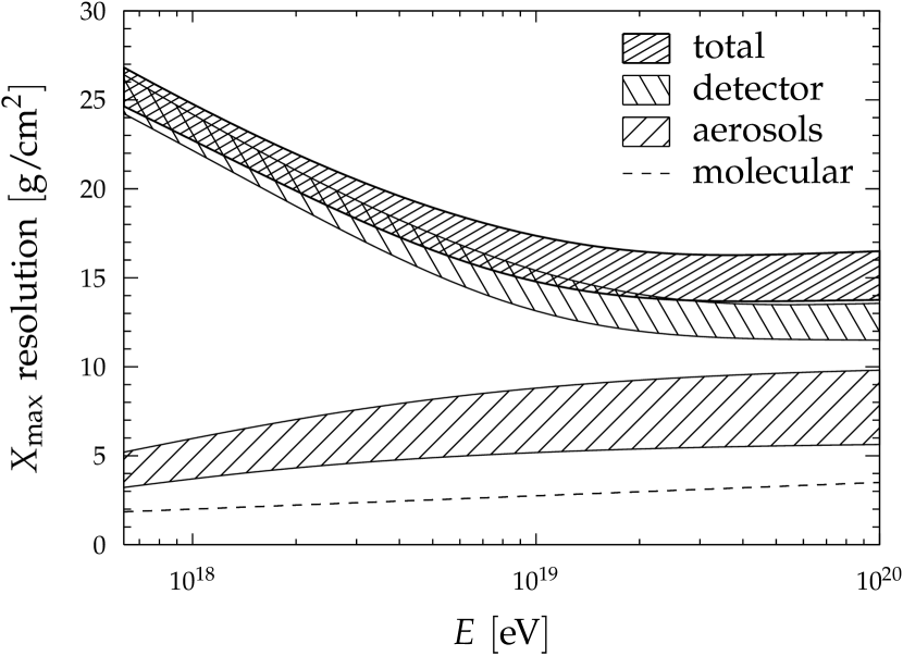
Another detector-related contribution to the resolution originates from the uncertainties in the alignment of the telescopes. These are estimated by comparing the values from two reconstructions of the data set with different alignment constants. One set of constants has been obtained using the traditional technique of observing tracks of UV stars (see, e.g., Sadowski:2002ij ) and the other one used shower geometries from events reconstructed with the surface detector for a cross-calibration. The latter are the default constants in the standard reconstruction. Averaged over all 24 telescopes, the values between events from the two reconstructions are found to be compatible, but systematic alignment differences are present on a telescope-by-telescope basis giving rise to a standard deviation of that amounts to . This is used as an estimate of the contribution of the telescope alignment to the resolution by adding to the previously discussed statistical part of the detector resolution in quadrature.
Finally, uncertainties in the relative timing between the FD and the SD can introduce additional uncertainties, but even for GPS jitters as large as 100 ns the effect on the resolution is 3 and can thus be neglected.
The estimated overall contribution of the detector-related uncertainties to the resolution is shown as a back-slashed band in Fig. 6.
VI.2 Aerosols
Two sources of statistical uncertainty of the aerosol measurements contribute to the resolution. Firstly, the measurement itself is affected by fluctuations of the night sky background and the number of photons received from the laser as well as by the time-variability of the aerosol content within the one-hour averages. The sum of both contributions is estimated using the standard deviation of the quarter-hourly measurements Abreu:2013qtw ; ValoreICRC13 of the VAOD and propagated to the uncertainty during reconstruction. Secondly, non-uniformities of the aerosol layers across the array are estimated using the differences of the VAOD measurements from different FD sites and propagated to an uncertainty Abraham:2010pf .
The quadratic sum of both sources is shown as the lowest of the dashed bands in Fig. 6, where the systematic uncertainty given by the width of the band is due to the uncertainty of the contribution from the horizontal non-uniformity.
VI.3 Molecular Atmosphere
Finally, the precision to which the density profiles as a function of height are known gives another contribution to the resolution. It is estimated from the spread of differences between shower reconstructions using the density profile from GDAS and shower reconstructions using actual balloon soundings, which are available for parts of the data (see Fig. 14 in Abreu:2012zg ). This contribution is shown as a dashed line in Fig. 6.
VI.4 Parameterization of the Resolution
The statistical part of the detector resolution arises from the statistical uncertainty in the determination of and from the statistical uncertainty caused by the conversion from the height of the maximum in the atmosphere to the corresponding depth of . Simulations of these two contributions show that they are well-described by the sum of two Gaussian distributions. The remaining component to the resolution term of Eq. (4) is also Gaussian and describes the contributions from the calibration of the detector and from the influence of the atmosphere. The overall resolution of can therefore be parameterized as
| (8) |
were denotes a Gaussian distribution with mean zero and width . The three parameters , and are listed in Tab. B as a function of energy together with their systematic uncertainties.
VII Moments
The parameterized acceptance and resolution together with the measured distributions provide the full information on the shower development for any type of physics analysis. However, the first two moments of the distribution, and , provide a compact way to characterize the main features of the distribution. In this section we describe three methods that have been explored to derive the moments from our data.
VII.1 Event Weighting
In this approach each selected shower is weighted according to the acceptance corresponding to the position of the shower maximum. Events in the region of constant acceptance are assigned a weight of one. The under-representation of the distribution in the non-flat part is compensated for by assigning the inverse of the relative acceptance as a weight to showers detected in this region, , cf. (7). The unbiased moments can be reconstructed using the equations for the weighted moments (cf. A.1). is then estimated by subtracting the resolution in quadrature from the weighted standard deviation.
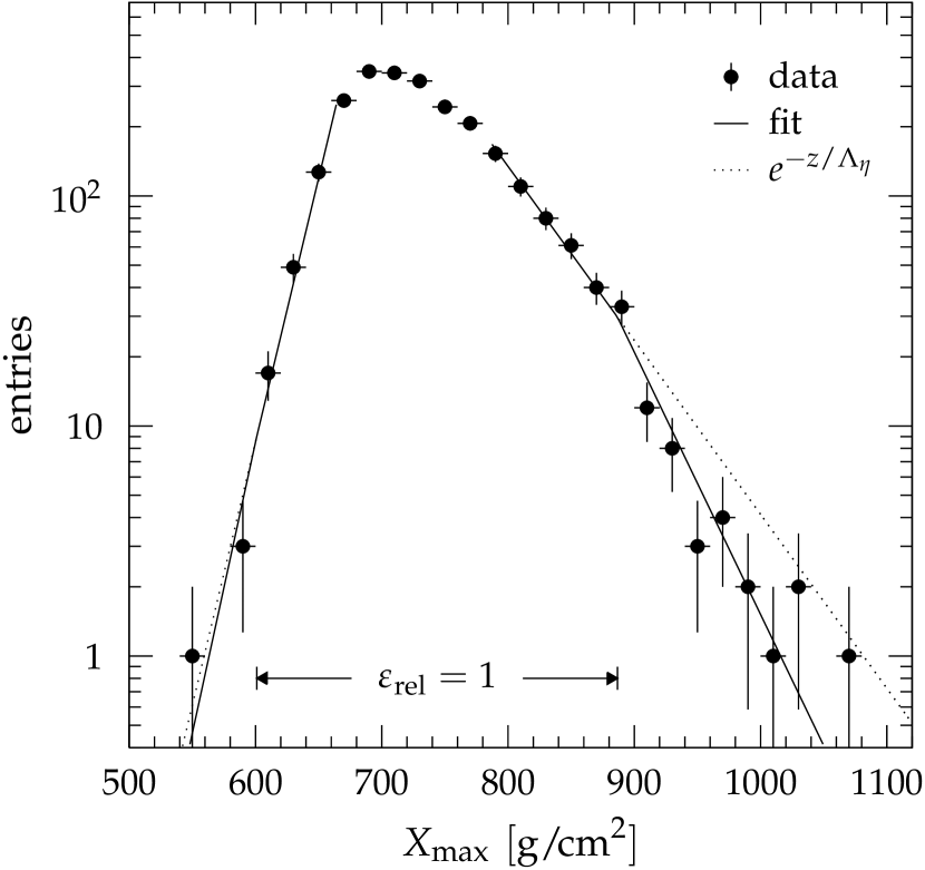
VII.2 method
The tail of the distribution at large values is related to the distribution of the first interactions of the primary particles in the atmosphere (see, e.g., Ulrich:2009zq ). Therefore, it is possible to describe the true distribution of deep showers by an exponential function. We subdivide the measured distribution into three regions: the central part with a constant acceptance, where the distribution can be measured without distortions, and the shallow and deep regions where the relative acceptance departs from unity. Here, for the purpose of calculating the first two moments of the distribution, the data are replaced by an exponential function that has been fitted to the two tails of the distribution, taking the acceptance into account (see A.2). A fraction of the events in the tail is fitted to obtain the slope , similar to the method that has been used previously to estimate the interaction length of proton-air collisions Baltrusaitis:1984ka ; Abreu:2012wt . The mean and standard deviation of the distribution are then calculated by combining the moments of the undistorted region with the exponential prolongation in the tails. In practice, since the distributions have a steep rising edge, the low- part is almost fully contained within the fiducial field of view and only the exponential tail at deep values contributes to a correction with respect to the moments calculated without taking into account the acceptance. In the final step, is obtained by subtracting the resolution in quadrature from the variance derived with this procedure.
VII.3 Deconvolution
As a third method we investigated the possibility to solve Eq. (4) for the true distribution and to subsequently determine the mean and variance of the solution. For this purpose, Eq. (4) can be transformed into a matrix equation by a piece-wise binning in and then be solved by matrix inversion. To overcome the well-known problem of large variances and negative correlations inherent to this approach (see, e.g., Cowan:2002in ), we applied two different deconvolution algorithms to the data, namely regularized unfolding using singular value decomposition (SVD) of the migration matrix Hocker:1995kb and iterative Bayesian deconvolution D'Agostini:1994zf .
VII.4 Comparison
Each of these three methods has its own conceptual advantages and disadvantages. The main virtue of the event weighting is that it is purely data-driven. However, with the help of simulated data it was found that this approach has the largest statistical variance of the three methods, resulting from large weights that inevitably occur when a shower is detected in a low-acceptance region.
The estimators of the moments resulting from the -method are also mainly determined by the measured data since the fiducial field of view ensures that only the small part of the distribution outside the range of constant acceptance needs to be extrapolated. The description of the tail of the distribution with an exponential function has a sound theoretical motivation. Obviously, this method is not applicable when the main part of the distribution is affected by distortions from the acceptance.
Deconvolution is in principle the most mathematically rigorous method to correct the measured distributions for the acceptance and resolution. However, in order to cope with the large variance of the exact solution, unfolding algorithms need to impose additional constraints to the data (such as minimal total curvature Tihonov:1963 in case of the SVD approach), that are less physically motivated than, e.g., an exponential prolongation of the distribution.
In the following we will use the -method as the default way to estimate the moments of the distribution. A comparison with the results of the other methods will be discussed in Sec. IX. It is worthwhile noting that the moments calculated without taking into account the acceptance are close to the ones estimated by the three methods described above, i.e., in the range of for and for . Assuming a perfect resolution would change by . Thus, the estimates of and are robust with respect to uncertainties on the acceptance and resolution.
VIII Systematic Uncertainties
VIII.1 Scale
The systematic uncertainty of the scale, i.e., the precision with which the absolute value of can be measured, is shown in Fig. 7. As can be seen, this uncertainty is at all energies. At low energies, the scale uncertainty is dominated by the uncertainties in the event reconstruction and at high energies the atmospheric uncertainties prevail. The different contributions to the scale uncertainty are discussed in the following. The full covariance matrix of the scale uncertainty is available at xmaxDataURL .
Detector Calibration
The uncertainties in the relative timing between the FD sites and SD stations, the optical alignment of the telescopes and the calibration of the absolute gains of photomultipliers of the cameras have been found to give only a minor contribution to the scale uncertainty. Their overall contribution is estimated to be less than 3 by evaluating the stability of the reconstruction under a variation of the relative timing by its uncertainty of ns augerTiming , using different versions of the gain calibration and by application of an independent set of alignment constants (cf. Sec. VI.1).
Reconstruction
The reconstruction algorithms described in Sec. III are tested by studying the average difference between the reconstructed and generated for simulated data. The bias is found to be less than 3.5 and is corrected for during data analysis. The dependence of the results on the particular choice of function fitted to the longitudinal profile has been checked by replacing the Gaisser-Hillas function from Eq. (5) by a Gaussian distribution in shower age , yielding compatible results within 4 for either of the variants proposed in AbuZayyad:2000np and gillerGia . Furthermore, we tested the influence of the constraints and used in the Gaisser-Hillas fit by altering their values by the standard deviations given in Sec. III, which changes the on average by less than 3.7 . Since the values obtained in these three studies (bias of simulated data, Gaussian in age and variation of constraints) are just different ways of assessing the same systematic effect, we do not add them in quadrature but assign the maximum deviation of 4 as an estimate of the scale uncertainty originating from the event reconstruction.
In addition to this validation of the reconstruction of the longitudinal shower development, we have also studied our understanding of the lateral distribution of fluorescence and Cherenkov light and its image on the FD cameras. For this purpose, the average of the light detected outside the collection angle in data is compared to the amount of light expected due to the point spread function of the optical system and the lateral distribution of the light from the shower. We find that the fraction of light outside is larger in data than in the expectation and that the ratio of observed-to-expected light depends on shower age. The corresponding correction of the data during the reconstruction leads to a shift of of at eV which decreases to at the highest energies. Since the reason for the mismatch between the observed and expected distribution of the light on the camera is not understood, the full shift is included as a one-sided systematic uncertainty. With the help of simulated data we estimated the precision with which the lateral-light distribution can be measured. This leads to a total uncertainty from the knowledge of the lateral-light distribution of at eV and at the highest energies.
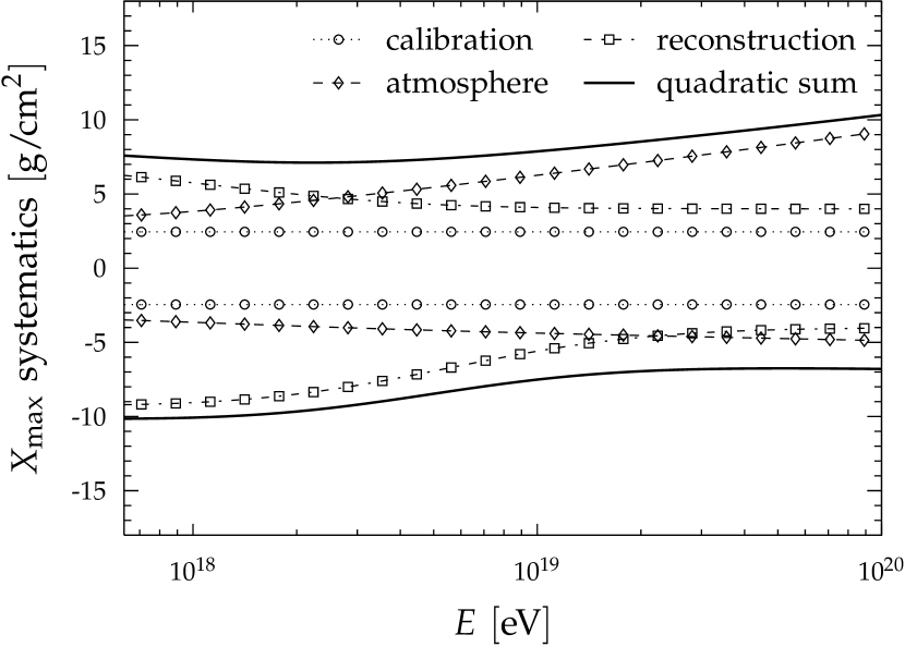
Atmosphere
The absolute yield of fluorescence-light production of air showers in the atmosphere is known with a precision of 4% Ave:2012ifa . The corresponding uncertainty of the relative composition of fluorescence and Cherenkov light leads to an uncertainty on the shape of the reconstructed longitudinal profiles and an uncertainty of 0.4 . Moreover, the uncertainty in the wavelength dependence of the fluorescence yield introduces an uncertainty of 0.2 . The amount of multiply-scattered light to be taken into account during the reconstruction depends on the shape and size of the aerosols in the atmosphere. In Louedec:2013caa the systematic effect on the scale has been estimated to be . The systematic uncertainty of the measurement of the aerosol concentration and its horizontal uniformity are discussed in Abraham:2010pf ; Abreu:2013qtw ; ValoreICRC13 . They give rise to an energy-dependent systematic uncertainty of , since high-energy showers can be detected at large distances and have a correspondingly larger correction for the light transmission between the shower and the detector. Thus, at the highest energies the scale uncertainty is dominated by uncertainty of the atmospheric monitoring, contributing in the last energy bin.
VIII.2 Moments
The systematic uncertainties of and are dominated by the scale uncertainty and by the uncertainty of the resolution, respectively, which have been discussed previously (Sec. VIII and VI).
In addition, the uncertainties of the parameters of the acceptance, Eq. (7), are propagated to obtain the corresponding uncertainties of the moments leading to and for and , respectively.
Finally, we have also studied the possible bias of the moments originating from the difference in invisible energy between heavy and light primaries. In the energy reconstruction, the average invisible energy is corrected for. If the primary flux is composed of different nuclei, then the energy of heavy nuclei will be systematically underestimated and the one of light nuclei will be overestimated on an event-by-event basis. As a consequence, the single-nuclei spectra as a function of reconstructed energy will be shifted with respect to each other and the fraction of nuclei in a bin of reconstructed energy will be biased. To study consequences of this fraction bias on the moments, we consider the extreme case of a mixture of proton and iron primaries and an invisible energy as predicted by the Epos-LHC model. The observed energy spectrum after selection follows, to a good approximation, a power law with a spectral index . The potential bias of the moments due to the invisible energy correction is then found to be and which we add as a one-sided systematic uncertainty of the estimated moments.
IX Cross-Checks
The systematic uncertainties estimated in the previous section have been carefully validated by performing numerous cross-checks on the stability of the results and the description of the data by the detector simulation. In the following we present a few of the most significant studies.
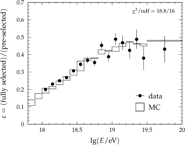
IX.1 Selection Efficiency
A potential bias from the quality and fiducial selection can be checked by comparing its efficiency as a function of energy for data and simulated events. For this purpose, we use the independent measurement of air showers provided by the SD and measure the fraction of events surviving the quality and fiducial cuts out of the total sample of pre-selected events. This estimate of the selection efficiency is shown in Fig. 8 as a function of SD energy above eV. Below that energy, the SD trigger efficiency drops below 50%. The comparison to the simulated data shows a good overall agreement and we conclude that the selection efficiency is fully described by our simulation.
IX.2 Detector Resolution
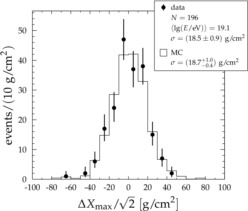
The understanding of the detector resolution is checked with the help of showers that had been detected by more than one FD site. The distribution of the differences in as reconstructed for each site independently gives an estimate of the resolution. As can be seen in Fig. 9, the distribution of the data and its standard deviation agrees well with the one obtained for simulated air showers.
IX.3 Analysis of Simulated Data
The full analysis chain can be validated by applying it to simulated data and comparing the estimated moments to the ones at generator level. This test has been performed in two variants. In the first test, we re-evaluated the fiducial field-of-view cuts from the simulated data to obtain the optimal boundaries with the algorithm described in Sec. IV.2. Furthermore, we also tested the performance when applying the range of the fiducial fields of view derived from the real data (cf. Eq. (6)). This second test is more conservative as it validates the ability of the analysis chain to recover the true moments of input distributions it has not been optimized for. This is an important feature needed for the comparison of the data to distributions that differ from the observed ones, e.g., for fitting different composition hypotheses to the data (cf. fractionPaper ).
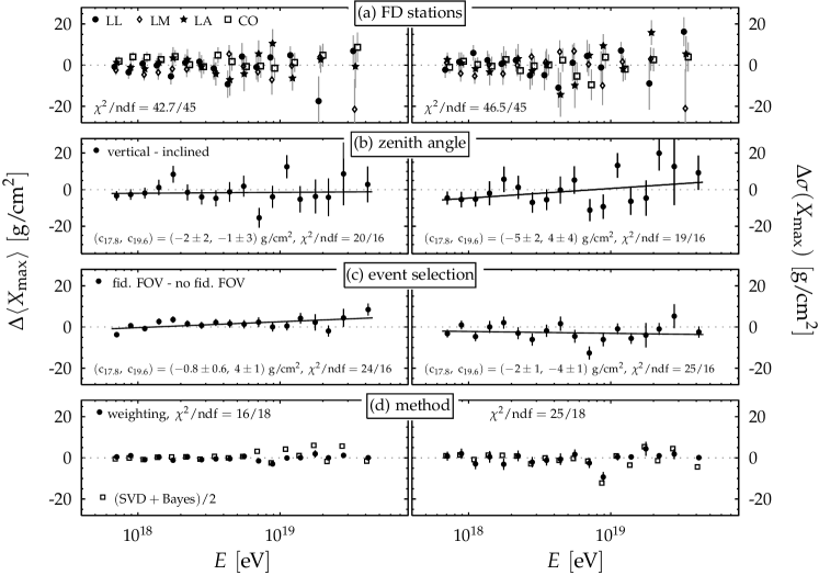
In both cases, the moments of the input distribution can be reproduced well. The results from the test using the field-of-view cuts from Eq. (6) are shown in Fig. 11. As can be seen, the simulated measurements of and agree within 2 with the generated values in case of a pure-proton or pure-iron composition. Slightly larger biases are visible for a mixed composition with 50% proton and 50% iron where deviates by about from the generated value. This bias can be partially attributed to the systematic uncertainty of the acceptance correction and the application of the average invisible-energy correction during the reconstruction (cf. Sec. VIII.2). We conclude that the analysis chain performs well, even for the case where the cuts of the fiducial fields-of-view are not re-optimized to the input distributions.
IX.4 FD Sites
The moments of the distribution can be measured for each of the four FD sites separately to check for possible differences due to misalignment or systematic differences in the PMT calibration. Moreover, the four sites (denoted as LL, LM, LA and CO in the following) are located at different altitudes with a maximum difference between LL at 1416.2 m and CO at 1712.3 m above sea level. Correspondingly, the aerosols, which have usually their largest concentration near ground level, are less important for CO than for the other sites. The results can be seen in Fig. 11 (a), where the differences of the individual and with respect to the results from the full data sample are shown. A test of the compatibility with zero yields 42.7 and 46.5 for and , respectively. Taking into account that the comparison is done with the mean of the data, the number of degrees of freedom is 45 in each case and it can therefore be concluded that the measurements at the individual sites are indeed statistically-independent estimates of the same quantity. Averaging the -values over energy for each station, the maximum deviation from zero is found to be for the measured in CO, which is well within the systematic uncertainties for calibration and aerosols listed in Sec. VIII.
IX.5 Zenith Angle
The electromagnetic part of an air shower develops as a function of traversed air mass. Therefore, the position of the shower maximum expressed in slant depth does not depend on the zenith angle of the arrival direction of the cosmic-ray particle. Accordingly, and are also expected to be independent of the zenith angle.
However, showers at different zenith angles reach their maximum at different heights above the ground and in different regions of the detector acceptance. Therefore, the study of a possible zenith-angle dependence of the moments of the distribution provides an important end-to-end cross-check of the understanding of the atmosphere and the detector.
For the purpose of this check, the data set is divided into two subsamples of approximately equal size at the median zenith angle and the acceptance and resolution are re-evaluated for these samples. This yields estimates of the moments for the “near-vertical” and “inclined” data and their difference is shown in Fig. 11 (b). No significant difference is found over the whole energy range for . At low energies, the near-vertical is smaller by about than the inclined one. Assuming that either one of the two subsamples gives a fair estimate of the true width, the corresponding bias of the full data sample would be , which is compatible with the systematic uncertainty of the combined at low energies.
IX.6 Event Selection
The dependence of the results on details of the fiducial field of view as well as on the acceptance and resolution is studied by completely removing the fiducial field-of-view selection. The data selected in this way is then corrected with the appropriate acceptance and resolution using the event weighting method. The difference from the default moments is shown in Fig. 11 (c), where the error bars take into account the correlation between the results due to the fact that they partially share the same events. As can be seen, the differences are within 4 on average for both, and . Due to the larger importance of the acceptance correction in the case of estimating the moments without fiducial cuts, it is expected that the corresponding systematic uncertainties are larger than the ones discussed in Sec. VIII. Moreover, the resolution of this selection is worse than the default discussed in Sec. VI. Given these differences, we conclude that the two results are in good overall agreement.
IX.7 Analysis Method
The different methods for the estimation of the moments that were introduced in Sec. VII are compared in Fig. 11 (d). The event-weighting yields results that are very similar to the -method. The presented statistical uncertainties account for the correlation of the two estimates which use exactly the same data set. The results of the two methods are found to be compatible with a of 0.9 and 1.4 for and , respectively.
The moments calculated from the deconvoluted distributions using either the Bayesian or SVD method were found to be compatible within 1 . Therefore, in Fig. 11 (d) the differences from the default result are shown for the arithmetic average of the two. As can be seen, they scatter around zero with no visible systematic trend. The statistical uncertainties of these differences have not been evaluated, but an estimate of their variances can be obtained by assuming proportionality to the statistical uncertainties of the default results. A of 1 is obtained when uncertainties are assumed to be 59% and 90% of those given in Tab. B for and , respectively. Therefore, it can be concluded that the moments obtained by deconvolution agree with the default results within the statistical uncertainties of the latter.
X Results and Discussion
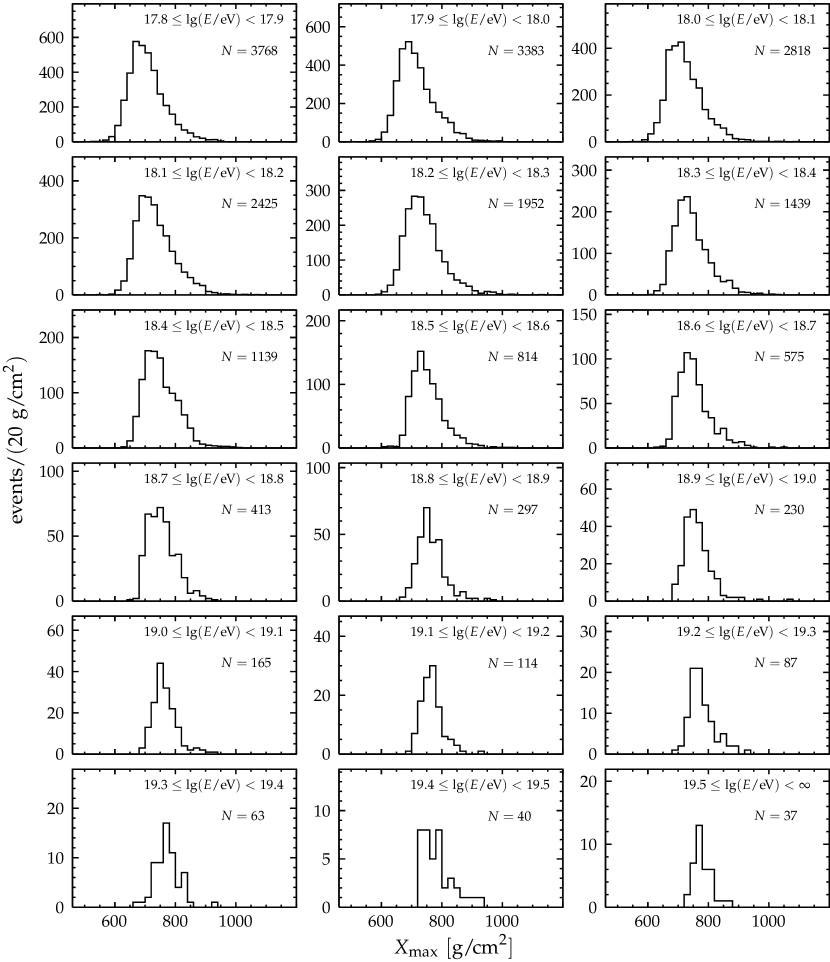
In the following we present the results of this analysis in energy bins of . Above eV an integral bin is used. The highest-energy event in this data sample had been detected by all four FD sites and its reconstructed energy and shower maximum are eV and , respectively, where the uncertainties are statistical only.
The distributions after event selection are shown in Fig. 12. These are the “raw” distributions ( in Eq. (4)) that still include effects of the detector resolution and the acceptance. Electronically readable tables of the distributions, as well as the parameters of the resolution and acceptance, are available at xmaxDataURL . A thorough discussion of the distributions can be found in an accompanying paper fractionPaper , where a fit of the data with simulated templates for different primary masses is presented.
In this paper we will concentrate on the discussion of the first two moments of the distribution, and , which are listed in Tab. B together with their statistical and systematic uncertainties. The statistical uncertainties are calculated with the parametric bootstrap method. For this purpose, the data are fitted with Eq. 4 assuming the functional form suggested in Peixoto:2013tu as . Given this parametric model of the true distribution, realizations of the measurement are repeatedly drawn from Eq. 4 with the number of events being equal to the ones observed. After application of the analysis described in Sec. VII.2, distributions of and are obtained from which the statistical uncertainties of the measured moments are estimated.
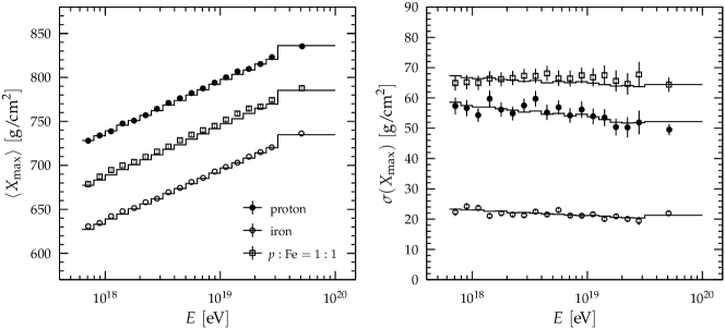
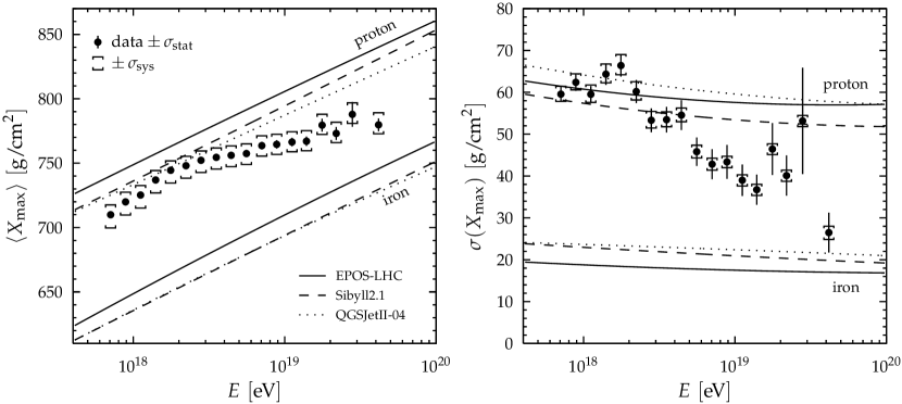
A comparison of the predictions of the moments from simulations for proton- and iron-induced air showers to the data is shown in Fig. 13. The simulations have been performed using the three contemporary hadronic interaction models that were either tuned to recent LHC data (QGSJetII-04 Ostapchenko:2010vb ; sergeiICRC11 , Epos-LHC Pierog:2006qv ; Pierog:2013ria ) or found in good agreement with these measurements (Sibyll2.1 Ahn:2009wx , see d'Enterria:2011kw ). It is worth noting that the energy of the first data point in Fig. 13 corresponds to a center-of-mass energy that is only four times larger than the one currently available at the LHC (). Therefore, unless the models have deficiencies in phase-space regions that are not covered well by LHC measurements, the uncertainties due to the extrapolation of hadronic interactions to the lower energy threshold of this analysis should be small. On the other hand, the last energy bin at corresponds to a center-of-mass energy that is a factor of about 40 higher than the LHC energies and the model predictions have to be treated more carefully.
Comparing the energy evolution of for data and simulations in Fig. 13 it can be seen that the slope of the data is different than what would be expected for either a pure-proton or pure-iron composition. The change of with the logarithm of energy is usually referred to as elongation rate elong1 ; elong2 ; elong3 ,
| (9) |
Within the superposition model, where it is assumed that a primary nucleus of mass and energy can be to a good approximation treated as a superposition of nucleons of energy , the elongation rate is expected to be the same for any type of primary. Any deviation of an observed elongation rate from this expectation can be attributed to a change of the primary composition,
| (10) |
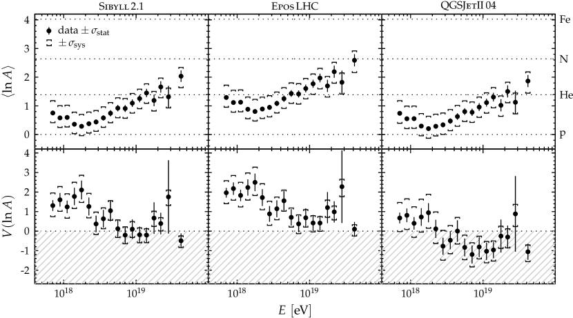
A single linear fit of as a function of does not describe our data well (). Allowing for a change in the elongation rate at a break point yields a good of with an elongation rate of
| (11) |
below and
| (12) |
above this energy. The average shower maximum at is . Here the systematic uncertainties on have been obtained by varying the individual contributions of the systematic uncertainties on separately.
The elongation rates predicted by air-shower simulations for a constant composition range from 54 to 64 /decade. Together with the results in Eqs. (11) and (12) we can therefore deduce that
| (13) |
below and
| (14) |
above this energy. This implies that there is an evolution of the average composition of cosmic rays towards lighter nuclei up to energies of eV. Above this energy, the trend reverses and the composition becomes heavier.
A similar behavior is visible for the width of the distribution in the right panel of Fig. 13, where it can be seen that the gets narrower towards high energies, as it would be expected for showers induced by heavy nuclei.
For a more quantitative study of the evolution of the composition,
and are converted to the first two moments of the
distribution (cf. Eq. (3)) following the
method described in Abreu:2013env ; AhnICRC13 . The mean and variance of
are shown in Fig. 14 using air-shower simulations
with three interaction models. As can be seen for all three cases, the
composition is lightest at around eV and the different
features of hadronic interactions implemented in the three models give
rise to differences in of about . The interpretation
with Epos-LHC leads to the heaviest average composition that is
compatible with the of nitrogen at the highest energies. The
variance of derived with Epos-LHC and Sibyll2.1 suggests
that the flux of cosmic rays is composed of different nuclei at low
energies and that it is dominated by a single type of nucleus above
eV where the variance, , is close to zero. The
interpretation with QGSJetII-04 leads to unphysical variances () above eV and therefore this model is disfavored by
our data, unless one allows for a systematic bias that is twice as
large as the uncertainties estimated in Sec. VIII.
XI Conclusions
In this paper, we presented the measurement of the distribution of the depth of shower maximum of ultra-high energy cosmic-ray air showers. We described the data selection which allows for a nearly unbiased measurement of the distributions and discussed the residual effects of acceptance and resolution. The data set is the largest sample of measurements hitherto collected by a cosmic-ray detector. We provide computer-readable tables of the distributions and detector parameters that make it possible to interpret the measurements without the need of additional software to simulate the detector response. This approach will also facilitate the comparison with measurements of from other experiments Barcikowski:2013nfa . Here we cannot provide such a comparison, since for these data neither the detector bias is controlled for using fiducial cuts, nor are the resolution and acceptance publicly available.
An interpretation in terms of mass composition of the moments of the distribution was given using air-shower simulations with contemporary hadronic interaction models. Assuming that the modeling of hadronic interactions gives a fair representation of the actual processes in air showers at ultra-high energies, our data suggest that the flux of cosmic rays is composed of predominantly light nuclei at around eV and that the fraction of heavy nuclei is increasing up to energies of eV. Estimates of the fractions of groups of nuclei contributing to the cosmic-ray flux can be derived by interpreting the full distributions. Such an analysis can be found in an accompanying paper fractionPaper .
XII Acknowledgments
The successful installation, commissioning, and operation of the Pierre Auger Observatory would not have been possible without the strong commitment and effort from the technical and administrative staff in Malargüe.
We are very grateful to the following agencies and organizations for financial support:
Comisión Nacional de Energía Atómica, Fundación Antorchas, Gobierno De La Provincia de Mendoza, Municipalidad de Malargüe, NDM Holdings and Valle Las Leñas, in gratitude for their continuing cooperation over land access, Argentina; the Australian Research Council; Conselho Nacional de Desenvolvimento Científico e Tecnológico (CNPq), Financiadora de Estudos e Projetos (FINEP), Fundação de Amparo à Pesquisa do Estado de Rio de Janeiro (FAPERJ), São Paulo Research Foundation (FAPESP) Grants # 2010/07359-6, # 1999/05404-3, Ministério de Ciência e Tecnologia (MCT), Brazil; MSMT-CR LG13007, 7AMB14AR005, CZ.1.05/2.1.00/03.0058 and the Czech Science Foundation grant 14-17501S, Czech Republic; Centre de Calcul IN2P3/CNRS, Centre National de la Recherche Scientifique (CNRS), Conseil Régional Ile-de-France, Département Physique Nucléaire et Corpusculaire (PNC-IN2P3/CNRS), Département Sciences de l’Univers (SDU-INSU/CNRS), Institut Lagrange de Paris, ILP LABEX ANR-10-LABX-63, within the Investissements d’Avenir Programme ANR-11-IDEX-0004-02, France; Bundesministerium für Bildung und Forschung (BMBF), Deutsche Forschungsgemeinschaft (DFG), Finanzministerium Baden-Württemberg, Helmholtz-Gemeinschaft Deutscher Forschungszentren (HGF), Ministerium für Wissenschaft und Forschung, Nordrhein Westfalen, Ministerium für Wissenschaft, Forschung und Kunst, Baden-Württemberg, Germany; Istituto Nazionale di Fisica Nucleare (INFN), Ministero dell’Istruzione, dell’Università e della Ricerca (MIUR), Gran Sasso Center for Astroparticle Physics (CFA), CETEMPS Center of Excellence, Italy; Consejo Nacional de Ciencia y Tecnología (CONACYT), Mexico; Ministerie van Onderwijs, Cultuur en Wetenschap, Nederlandse Organisatie voor Wetenschappelijk Onderzoek (NWO), Stichting voor Fundamenteel Onderzoek der Materie (FOM), Netherlands; National Centre for Research and Development, Grant Nos.ERA-NET-ASPERA/01/11 and ERA-NET-ASPERA/02/11, National Science Centre, Grant Nos. 2013/08/M/ST9/00322, 2013/08/M/ST9/00728 and HARMONIA 5 - 2013/10/M/ST9/00062, Poland; Portuguese national funds and FEDER funds within COMPETE - Programa Operacional Factores de Competitividade through Fundação para a Ciência e a Tecnologia, Portugal; Romanian Authority for Scientific Research ANCS, CNDI-UEFISCDI partnership projects nr.20/2012 and nr.194/2012, project nr.1/ASPERA2/2012 ERA-NET, PN-II-RU-PD-2011-3-0145-17, and PN-II-RU-PD-2011-3-0062, the Minister of National Education, Programme for research - Space Technology and Advanced Research - STAR, project number 83/2013, Romania; Slovenian Research Agency, Slovenia; Comunidad de Madrid, FEDER funds, Ministerio de Educación y Ciencia, Xunta de Galicia, European Community 7th Framework Program, Grant No. FP7-PEOPLE-2012-IEF-328826, Spain; Science and Technology Facilities Council, United Kingdom; Department of Energy, Contract No. DE-AC02-07CH11359, DE-FR02-04ER41300, DE-FG02-99ER41107 and DE-SC0011689, National Science Foundation, Grant No. 0450696, The Grainger Foundation, USA; NAFOSTED, Vietnam; Marie Curie-IRSES/EPLANET, European Particle Physics Latin American Network, European Union 7th Framework Program, Grant No. PIRSES-2009-GA-246806; and UNESCO.
References
- (1) J. Linsley, Proc. 8th ICRC 4 (1963) 77.
- (2) A. M. Hillas, J. Phys. G31 (2005) R95.
- (3) D. Allard, E. Parizot, A. V. Olinto, Astropart. Phys. 27 (2007) 61.
- (4) R. Aloisio et al., Astropart. Phys. 27 (2007) 76.
- (5) R. U. Abbasi et al. [HiRes Collaboration], Phys. Rev. Lett. 100 (2008) 101101.
- (6) J. Abraham et al. [Pierre Auger Collaboration], Phys. Rev. Lett. 101 (2008) 061101.
- (7) T. Abu-Zayyad et al. [TA Collaboration], Astrophys. J. 768 (2013) L1.
- (8) K. Greisen, Phys. Rev. Lett. 16 (1966) 748.
- (9) G. T. Zatsepin, V. A. Kuzmin, JETP Lett. 4 (1966) 78.
- (10) B. Peters, Nuovo Cimento 22 (1961) 800.
- (11) D. Allard et al., JCAP 0810 (2008) 033.
- (12) R. Aloisio, V. Berezinsky, A. Gazizov, Astropart. Phys. 34 (2011) 620.
- (13) D. Hooper, A. M. Taylor, Astropart. Phys. 33 (2010) 151.
- (14) K. Fang, K. Kotera, A. V. Olinto, JCAP 1303 (2013) 010.
- (15) K.-H. Kampert, M. Unger, Astropart. Phys. 35 (2012) 660.
- (16) K. Greisen, Ann. Rev. Nucl. Part. Sci. 10 (1960) 63.
- (17) J. Linsley, Proc. 15th ICRC 12 (1977) 89.
- (18) T. K. Gaisser, T. J. K. McComb, K. E. Turver, Proc. 16th ICRC 9 (1979) 258.
- (19) J. Linsley, A. A. Watson, Phys. Rev. Lett. 46 (1981) 459.
- (20) J. Linsley, Proc. 18th ICRC 12 (1983) 135.
- (21) J. Linsley, Proc. 19th ICRC 6 (1985) 1.
- (22) J. Engel et al., Phys. Rev. D46 (11) (1992) 5013.
- (23) J. Matthews, Astropart. Phys. 22 (2005) 387.
- (24) R. Ulrich, R. Engel, M. Unger, Phys. Rev. D83 (2011) 054026.
- (25) R. D. Parsons, C. Bleve, S. S. Ostapchenko, J. Knapp, Astropart. Phys. 34 (2011) 832.
- (26) R. Engel, D. Heck, T. Pierog, Ann. Rev. Nucl. Part. Sci. 61 (2011) 467.
- (27) P. Abreu et al. [Pierre Auger Collaboration], Phys. Rev. Lett. 109 (2012) 062002.
- (28) J. W. Belz et al. [FLASH Collaboration], Astropart. Phys. 25 (2006) 129.
- (29) M. Ave et al. [AIRFLY Collaboration], Nucl. Instrum. Meth. A597 41.
- (30) G. L. Cassiday et al. [Fly’s Eye Collaboration], Astrophys. J. 356 (1990) 669.
- (31) R. U. Abbasi et al. [HiRes Collaboration], Astrophys. J. 622 (2005) 910.
- (32) R. U. Abbasi et al. [HiRes Collaboration], Phys. Rev. Lett. 104 (2010) 161101.
- (33) J. Abraham et al. [Pierre Auger Collaboration], Phys. Rev. Lett. 104 (2010) 091101.
- (34) G. Cowan, Conf. Proc. C0203181 (2002) 248.
- (35) J. Abraham et al. [Pierre Auger Collaboration], Nucl. Instrum. Meth. A523 (2004) 50.
- (36) I. Allekotte et al. [Pierre Auger Collaboration], Nucl. Instrum. Meth. A586 (2008) 409.
- (37) J. Abraham et al. [Pierre Auger Collaboration], Nucl. Instrum. Meth. A620 (2010) 227.
- (38) F. Sanchez et al. [Pierre Auger Collaboration], Proc. 32nd ICRC 3 (2011) 145.
- (39) H. J. Mathes et al. [Pierre Auger Collaboration], Proc. 32nd ICRC 3 (2011) 149.
- (40) A. Aab et al. [Pierre Auger Collaboration], in preparation.
- (41) J. T. Brack et al., Astropart. Phys. 20 (2004) 653.
- (42) A. C. Rovero et al. [Pierre Auger Collaboration], Astropart. Phys. 31 (2009) 305.
- (43) J. T. Brack et al., JINST 8 (2013) P05014.
- (44) NOAA Air Resources Laboratory (ARL), Global Data Assimilation System (GDAS1) Archive, Information, Tech. Rep. (2004), http://ready.arl.noaa.gov/gdas1.php.
- (45) P. Abreu et al. [Pierre Auger Collaboration], Astropart. Phys. 35 (2012) 591.
- (46) J. Abraham et al. [Pierre Auger Collaboration], Astropart. Phys. 33 (2010) 108.
- (47) B. Fick et al., JINST 1 (2006) P11003.
- (48) P. Abreu et al. [Pierre Auger Collaboration], JINST 8 (2013) P04009.
- (49) S. Y. BenZvi et al., Nucl. Instrum. Meth. A574 (2007) 171.
- (50) J. Chirinos et al. [Pierre Auger Collaboration], Proc. 33nd ICRC (2013), arXiv:1307.5059.
- (51) GOES Project Science, http://goes.gsfc.nasa.gov.
- (52) P. Abreu et al. [Pierre Auger Collaboration], Astropart. Phys. 50-52 (2013) 92.
- (53) S. Argiro et al., Nucl. Instrum. Meth. A580 (2007) 1485.
- (54) L. G. Porter et al., Nucl. Instrum. Meth. 87 (1970) 87.
- (55) P. Sommers, Astropart. Phys. 3 (1995) 349.
- (56) B. R. Dawson, H. Y. Dai, P. Sommers, S. Yoshida, Astropart. Phys. 5 (1996) 239.
- (57) C. Bonifazi et al. [Pierre Auger Collaboration], Proc. 29th ICRC 7 (2005) 17.
- (58) D. Gora et al., Astropart. Phys. 24 (2006) 484.
- (59) M. Giller, G. Wieczorek, Astropart. Phys. 31 (2009) 212.
- (60) J. Bäuml et al. [Pierre Auger Collaboration], Proc. 33nd ICRC (2013), arXiv:1307.5059.
- (61) V. Verzi et al. [Pierre Auger Collaboration], Proc. 33nd ICRC (2013), arXiv:1307.5059.
- (62) M. Roberts, J. Phys. G31 (2005) 1291.
- (63) J. Pekala et al., Nucl. Instrum. Meth. A605 (2009) 388.
- (64) M. Giller, A. Smialkowski, Astropart.Phys. 36 (2012) 166.
- (65) M. Giller et al., J. Phys. G 30 (2004) 97.
- (66) A. M. Hillas, J. Phys. G 8 (1982) 1461.
- (67) F. Nerling et al., Astropart. Phys. 24 (2006) 421.
- (68) S. Lafebre et al., Astropart. Phys. 31 (2009) 243.
- (69) M. Unger et al., Nucl. Instrum. Meth. A588 (2008) 433.
- (70) M. Ave et al. [AIRFLY Collaboration], Astropart. Phys. 28 (2007) 41.
- (71) M. Ave et al. [AIRFLY Collaboration], Astropart. Phys. 42 (2013) 90.
- (72) T. K. Gaisser, A. M. Hillas, Proc. 15th ICRC 8 (1977) 353.
- (73) M. J. Tueros et al. [Pierre Auger Collaboration], Proc. 33nd ICRC (2013), arXiv:1307.5059.
- (74) P. Abreu et al. [Pierre Auger Collaboration], Astropart. Phys. 34 (2011) 368.
- (75) P. Abreu et al. [Pierre Auger Collaboration], Astropart. Phys. 35 (2011) 266.
- (76) C. T. Peixoto, V. de Souza and J. Bellido, Astropart. Phys. 47 (2013) 18.
- (77) S. Andringa, R. Conceicao, M. Pimenta, Astropart. Phys. 34 (2011) 360.
- (78) T. Pierog, LHC data and extensive air showers, EPJ Web Conf. 52 (2013) 03001.
- (79) L. Prado et al., Nucl. Instrum. Meth. A545 (2005) 632.
- (80) T. Bergmann et al., Astropart. Phys. 26 (2007) 420.
- (81) E. J. Ahn et al., Phys. Rev. D80 (2009) 094003.
- (82) P. A. Sadowski et al. [HiRes Collaboration], Astropart. Phys. 18 (2002) 237.
- (83) L. Valore et al. [Pierre Auger Collaboration], Proc. 33nd ICRC (2013), arXiv:1307.5059.
- (84) R. Ulrich et al., New J. Phys. 11 (2009) 065018.
- (85) R. M. Baltrusaitis et al. [Fly’s Eye Collaboration], Phys. Rev. Lett. 52 (1984) 1380.
- (86) A. Höcker, V. Kartvelishvili, Nucl. Instrum. Meth. A372 (1996) 469.
- (87) G. D’Agostini, Nucl. Instrum. Meth. A362 (1995) 487.
- (88) A. N. Tihonov, Dokl. Akad. Nauk SSSR 151 (1963) 501.
- (89) A. Aab et al. [Pierre Auger Collaboration], http://www.auger.org/data/xmax2014.tar.gz.
- (90) P. Allison et al. [Pierre Auger Collaboration], Proc. 29th ICRC 8 (2005) 307.
- (91) T. Abu-Zayyad et al. [HiRes Collaboration], Astropart. Phys. 16 (2001) 1–11.
- (92) M. Giller et al., Proc. 29th ICRC 7 (2005) 187.
- (93) K. Louedec, J. Colombi, Astropart. Phys. 57 (2014) 58.
- (94) A. Aab et al. [Pierre Auger Collaboration], Depth of Maximum of Air-Shower Profiles at the Pierre Auger Observatory: Composition Implications, submitted to Phys. Rev. D (2014).
- (95) S. Ostapchenko, Phys. Rev. D83 (2011) 014018.
- (96) S. Ostapchenko, Proc. 32nd ICRC vol. 2 (2011) 71.
- (97) T. Pierog, K. Werner, Phys. Rev. Lett. 101 (2008) 171101.
- (98) T. Pierog et al., arXiv:1306.0121.
- (99) D. d’Enterria et al., Astropart. Phys. 35 (2011) 98.
- (100) P. Abreu et al. [Pierre Auger Collaboration], JCAP 1302 (2013) 026.
- (101) E. J. Ahn et al. [Pierre Auger Collaboration], Proc. 33nd ICRC (2013), arXiv:1307.5059.
- (102) E. Barcikowski et al. [HiRes, Pierre Auger, TA and Yakutsk Collaborations], EPJ Web Conf. 53 (2013) 01006.
Appendix A Calculation of Moments
A.1 Weighted Events
One possibility to correct for the acceptance as a function of is to assign to each event a weight . The average shower maximum of events weighted by the inverse of the acceptance is given by
| (15) |
The second non-central moment is
| (16) |
with which
| (17) |
where
| (18) |
giving us the usual factor of when all weights are equal to one.
A.2 -Method
When the shower maxima of the events in the tails of the distribution follow an exponential distribution, damped by an exponential acceptance above a certain depth (cf. Eq. (7)), then the resulting distribution of the upper tail is given by
| (19) |
and a similar formula describes the lower tail, where denotes the distance to the start point of the fit and is the distance above which the acceptance decreases exponentially with decay constant . The normalization is given by
| (20) |
The fraction of events in the tail is denoted by . Following Abreu:2012wt we use for the tail at large and the leading edge of the distribution is fitted using .
The unbinned likelihood for events in the tail is
| (21) |
where terms independent of have been omitted.
An illustration of a fit of the upper and lower tail of the distribution is shown in Fig. 15. The fitted damped exponential is shown as the solid line and the range of constant acceptance is indicated by arrows. For the purpose of calculating the moments, the data distribution is replaced by the exponential functions (shown as dashed lines) outside of the range.
Appendix B Data tables
| range | ||||
|---|---|---|---|---|
| 586 6 | 109 17 | 881 8 | 95 7 | |
| 592 9 | 133 17 | 883 8 | 101 7 | |
| 597 11 | 158 19 | 885 8 | 107 7 | |
| 601 14 | 182 21 | 887 8 | 113 7 | |
| 604 17 | 206 24 | 888 8 | 119 7 | |
| 605 20 | 230 28 | 890 8 | 125 7 | |
| 605 23 | 253 32 | 892 8 | 131 7 | |
| 604 27 | 276 38 | 894 9 | 137 8 | |
| 602 30 | 299 44 | 896 9 | 143 8 | |
| 599 33 | 321 51 | 898 9 | 150 8 | |
| 594 36 | 344 59 | 899 9 | 156 8 | |
| 588 39 | 365 67 | 901 9 | 162 8 | |
| 581 43 | 386 77 | 903 9 | 168 8 | |
| 573 46 | 407 86 | 905 9 | 174 8 | |
| 563 49 | 428 98 | 907 9 | 180 8 | |
| 553 52 | 447 109 | 908 9 | 186 8 | |
| 540 56 | 468 122 | 910 9 | 192 8 | |
| 517 62 | 502 146 | 913 10 | 203 9 |