Non-Radial Instabilities and Progenitor Asphericities in Core-Collapse Supernovae

Abstract

Since core-collapse supernova simulations still struggle to produce robust neutrino-driven explosions in 3D, it has been proposed that asphericities caused by convection in the progenitor might facilitate shock revival by boosting the activity of non-radial hydrodynamic instabilities in the post-shock region. We investigate this scenario in depth using 42 relativistic 2D simulations with multi-group neutrino transport to examine the effects of velocity and density perturbations in the progenitor for different perturbation geometries that obey fundamental physical constraints (like the anelastic condition). As a framework for analysing our results, we introduce semi-empirical scaling laws relating neutrino heating, average turbulent velocities in the gain region, and the shock deformation in the saturation limit of non-radial instabilities. The squared turbulent Mach number, $\langle\mathrm{Ma}^{2}\rangle$, reflects the violence of aspherical motions in the gain layer, and explosive runaway occurs for $\langle\mathrm{Ma}^{2}\rangle\gtrsim 0.3$, corresponding to a reduction of the critical neutrino luminosity by $\mathord{\sim}25\%$ compared to 1D. In the light of this theory, progenitor asphericities aid shock revival mainly by creating anisotropic mass flux onto the shock: Differential infall efficiently converts velocity perturbations in the progenitor into density perturbations $\delta\rho/\rho$ at the shock of the order of the initial convective Mach number $\mathrm{Ma}_{\mathrm{prog}}$. The anisotropic mass flux and ram pressure deform the shock and thereby amplify post-shock turbulence. Large-scale ($\ell=2$, $\ell=1$) modes prove most conducive to shock revival, whereas small-scale perturbations require unrealistically high convective Mach numbers. Initial density perturbations in the progenitor are only of order $\mathrm{Ma}_{\mathrm{prog}}^{2}$ and therefore play a subdominant role.

1 Introduction

The core-collapse supernova explosion mechanism has remained one of the outstanding challenges in theoretical astrophysics for decades. Among the various mechanisms that have been proposed over the years to explain supernova explosions (see Janka 2012 and Burrows 2013 for an up-to-date summary), the delayed neutrino-driven mechanism currently remains the best explored and most promising scenario, at least for core-collapse supernovae with explosion energies not exceeding $\mathord{\sim}10^{51}\ \mathrm{erg}$. Throughout its long history, the idea of shock revival due to neutrino-heating has seen many refinements; in its modern form it relies on the joint action of neutrino heating and multi-dimensional hydrodynamic instabilities in the post-shock region, such as convection (Herant, Benz & Colgate, 1992; Burrows & Fryxell, 1992; Herant et al., 1994; Burrows, Hayes & Fryxell, 1995; Janka & Müller, 1996; Müller & Janka, 1997) and the standing accretion shock instability (SASI; Blondin, Mezzacappa & DeMarino, 2003; Marek & Janka, 2009 to revive the supernova shock. Over the recent years, an impressive set of successful two-dimensional (2D) multi-group neutrino hydrodynamics simulations (Buras et al., 2006a; Marek & Janka, 2009; Yakunin et al., 2010; Suwa et al., 2010; Müller, Janka & Marek, 2012; Müller, Janka & Heger, 2012; Janka et al., 2012; Bruenn et al., 2013; Suwa et al., 2013) has lent further credence to the idea of neutrino-driven supernova explosions.

However, even in the light of these recent successes of first-principle modelling in 2D, there are indications that our understanding of the neutrino-driven mechanism is still incomplete. It has yet to be demonstrated that the current 2D simulations are compatible with observed supernova explosion energies, nickel masses (Tanaka et al., 2009; Smartt, 2009; Utrobin & Chugai, 2011), and neutron star masses (Schwab, Podsiadlowski & Rappaport, 2010; Valentim, Rangel & Horvath, 2011; Özel et al., 2012; Kiziltan et al., 2013), although the explosion energies obtained by Bruenn et al. (2013) already fall roughly within the expected range. More importantly, parametrised studies of shock revival in core-collapse supernovae in 3D (Hanke et al., 2012; Couch, 2013a), as well as fully-fledged 3D neutrino hydrodynamics simulations (Hanke et al., 2013; Takiwaki, Kotake & Suwa, 2014) indicate that explosions may be harder to obtain in 3D (see, however, Dolence et al. 2013 for a differing opinion). Among the available 3D neutrino hydrodynamics simulations, those (Hanke et al., 2013; Tamborra et al., 2014) relying on what is currently the most rigorous approach to neutrino transport and the most comprehensive treatment of the neutrino microphysics still fail to show explosions. While it would be exaggerated to state that supernova theory has reached an impasse after progressing to 3D, this suggests that some important element for robust neutrino-driven explosions may yet be missing.

Motivated by these recent results on 3D effects in supernova cores, Couch & Ott (2013) proposed (extending ideas of Arnett & Meakin 2011) that large-scale asymmetries in the progenitor might support shock revival by instigating more violent aspherical motions in the post-shock region as they collapse and fall through the shock, thus adding a new twist to a problem at the interface between late-stage stellar evolution and supernova theory that has so far been studied primarily as a possible explanation for pulsar kicks (Burrows & Hayes, 1996; Goldreich, Lai & Sahrling, 1997; Lai & Goldreich, 2000; Fryer, Holz & Hughes, 2004; Murphy, Burrows & Heger, 2004). The idea of Couch & Ott (2013) certainly has a firm basis in late-stage stellar evolution: Seed asphericities will inevitable be present in the silicon and oxygen shell due to convective burning. A number of multi-D simulations of the pre-supernova phase suggest that convection in these shells is violent enough to produce significant density and velocity perturbations (Arnett, 1994; Bazan & Arnett, 1994, 1998; Asida & Arnett, 2000; Meakin & Arnett, 2007b, a; Arnett & Meakin, 2011), and those covering large 2D wedges (Meakin & Arnett, 2006, 2007a; Arnett & Meakin, 2011) or the full solid angle in 3D (Kuhlen, Woosley & Glatzmaier, 2003) show that large-scale modes indeed dominate the flow. In addition, the excitation of g-modes by shell burning (Goldreich, Lai & Sahrling, 1997) may produce asymmetries even within the iron core, although the analysis of Murphy, Burrows & Heger (2004) suggests that the growth time-scales for such unstable modes may be too long to produce large deviations from spherical symmetry.

Couch & Ott (2013) studied the effect of large-scale seed perturbations using 3D core-collapse simulations with a neutrino leakage scheme. In order to asses the impact of the progenitor asphericities, they computed models with and without initial perturbations, and with two different settings for a multiplicative factor regulating the neutrino heating term (not the net neutrino heating) in their leakage scheme. Among their four simulations, they found an explosion only for the case with initial perturbations with slightly enhanced neutrino heating. The similarity of their unperturbed model with enhanced neutrino heating (by $2\%$) and their perturbed model with the standard heating rate suggested a slight decrease of the critical luminosity required for shock revival.

While the idea of Couch & Ott (2013) is interesting, their work leaves a number of unanswered questions. Arguably, they find only a rather modest effect, which is just sufficient to tilt the balance in favour of an explosion in a marginal case. Moreover, Couch & Ott (2013) restricted their attention to a single perturbation pattern. In a recent follow-up paper (Couch & Ott, 2014), they simulated the same progenitor using ten different perturbation patterns, but a systematic exploration of the role of the perturbation geometry and amplitude is still lacking.

Furthermore, while taking some constraints on the convective velocities and the typical spatial scales from multi-D simulations of supernova progenitors into account (motivated by Arnett & Meakin 2011), Couch & Ott (2013, 2014) use purely transverse velocity perturbations which hardly resemble any convective flow pattern and even violate the important physical constraint of near-anelasticity for subsonic flow. Due to their use of a neutrino leakage scheme, the heating conditions also deviate considerably from simulations using a more elaborate neutrino treatment, at least during the later accretion phase after more than $150\ \mathrm{ms}$ after bounce.

In this study, we extend the work of Couch & Ott (2013, 2014) with a more systematic investigation of the role of progenitor asphericities from convective burning in the neutrino-driven mechanism. As we still lack multi-D progenitor models evolved up to the onset of collapse, we try to incorporate more physical constraints in our setup of the initial perturbation and also explore the effect of different perturbation amplitudes and geometries in detail. Unlike Couch & Ott (2013, 2014), we use a newly developed multi-group transport scheme based on a one-moment closure of the Boltzmann equation to ensure reasonable quantitative agreement with the most advanced multi-D neutrino hydrodynamics simulations. However, in order to explore the parameter space in depth with over 40 simulations, we restrict ourselves to axisymmetric 2D models. With this extensive parameter study, we attempt to address a number of questions concerning the role of progenitor asphericities in the explosion mechanism:

1. Can we better quantify the impact of progenitor asphericities on the conditions for shock revival?

2. How relevant is the spatial scale of the convective seed perturbations?

3. What are the minimum perturbation amplitudes required for an appreciable effect on the heating conditions?

4. Can we better understand the physical mechanism whereby perturbations facilitate shock revival?

In addition, we also pursue a second, subsidiary goal: In order to fully grasp the role of non-radial instabilities in the core-collapse supernova explosion mechanism, it is imperative that we develop a more quantitative understanding of the interplay of neutrino heating on the one hand and convection and/or the SASI on the other hand (regardless of whether seed asphericities in the progenitor are present or not). Several authors have already proposed theories to explain the saturation properties of the SASI (Guilet, Sato & Foglizzo, 2010) and of convection (Murphy & Meakin, 2011; Murphy, Dolence & Burrows, 2013), but, with the exception of Murphy, Dolence & Burrows (2013), no attempt has yet been made to break down these theories to simple scaling laws for volume-integrated quantities that can easily be extracted from multi-D simulations (total kinetic energies in non-spherical motions, volume-integrated neutrino heating rate, etc.). Furthermore, only Murphy, Dolence & Burrows (2013) undertook the first steps to explain the feedback of non-radial instabilities on the heating conditions quantitatively by analysing the effect of turbulent stresses on the average shock radius. We follow up on some of the ideas enunciated in the aforementioned papers better by formulating semi-empirical scaling laws relating neutrino heating, the violence of non-spherical instabilities, and the deformation of the shock. We also present some ideas about quantifying the effect of the non-spherical instabilities on the neutrino heating conditions and the critical luminosity for shock revival. Although we cannot hope to fully anatomise the interplay between neutrino heating and non-radial instabilities in this paper, we believe that the ideas formulated here may turn out helpful for the conceptual and quantitative understanding of the role of non-spherical instabilities in the supernova core in the future.

Our paper is organised as follows: In Section 2, we discuss a number of constraints on the multi-D structure of (non-rotating) supernova progenitors to provide some background information for the numerical setup of our simulations, which is detailed in Section 3. We then provide a cursory and descriptive overview of the effects of progenitor asphericities in our simulations in Section 4. The detailed analysis of our results is split in two Sections: In Section 5, we discuss the evolution of the unperturbed baseline model and establish quantitative relations governing the interplay between neutrino heating, non-radial motions in the post-shock region, and large-scale deformations of the shock. In Section 6, we then present a quantitative analysis of how progenitor asphericities modify the approach to an explosive runaway, describe the mechanism whereby progenitor asphericities facilitate shock revival, and discuss the dependence on the character and geometry of the initial perturbations. In Section 7, we summarise our results, discuss uncertainties and outline central questions for future research on the role of progenitor asphericities in core-collapse supernovae. Our paper also contains two appendices, the first of which (Appendix A) provides a detailed description of the fast multi-group transport (FMT) scheme used in our simulations. In Appendix B, we present a simple toy model for the effect of non-spherical instabilities on the explosion conditions.

2 Seed Perturbations in the Progenitor

While there have been a handful of multi-D simulations of Si-, O-, and C-shell burning during the late pre-collapse evolution (Arnett, 1994; Bazan & Arnett, 1994, 1998; Asida & Arnett, 2000; Kuhlen, Woosley & Glatzmaier, 2003; Meakin & Arnett, 2007b, a; Arnett & Meakin, 2011), we still lack multi-D progenitor models evolved all the way to collapse. For this reason, we are presently forced to impose seed perturbations onto 1D stellar evolution models by hand. Nevertheless multi-D simulations of the pre-collapse burning phases, mixing-length theory, and general physical principles still allow an informed judgement about the amplitude and the geometry of aspherical seed perturbations in the progenitor. In the following, we review a few of these principles in order to obtain some guidelines for constructing multi-D initial models before describing the initial perturbations used in our simulations.

2.1 Properties of Convective Regions in the Progenitor – Perturbation Amplitudes

Both mixing-length theory and multi-D simulations of convective burning in massive stars furnish estimates for the typical velocity and density perturbations in the silicon and oxygen shells. Depending on the dimensionality, the numerical methodology, and the inclusion or non-inclusion of multiple burning shells, the magnitude of the perturbations varies considerably: Bazan & Arnett (1998) reported relatively large typical Mach numbers of the order of $\mathrm{Ma}_{\mathrm{prog}}\sim 0.1\ldots 0.2$ and density fluctuations of up to $8\%$ in their 2D simulations of oxygen shell burning, whereas Kuhlen, Woosley & Glatzmaier (2003) found much smaller typical Mach numbers $\mathrm{Ma}_{\mathrm{prog}}\sim 0.01$ and density fluctuations $\delta\rho/\rho\sim(2\ldots 3)\times 10^{-3}$ in their pseudospectral 3D simulations relying on the anelastic approximation. In a detailed comparison of their compressible 2D and 3D models with the results of Kuhlen, Woosley & Glatzmaier (2003), Meakin & Arnett (2007a) ascribe these differences to the choice of boundary conditions, which, as they argue, prevented Kuhlen, Woosley & Glatzmaier (2003) from capturing large density perturbations at the convective boundaries associated with convective overshoot. Furthermore, Meakin & Arnett (2007a) found smaller typical Mach numbers in 3D compared to 2D (by a factor of $2\ldots 3$). However, the 3D results of Meakin & Arnett (2007a) were limited to a wedge of $30^{\circ}\times 30^{\circ}$ and did not include the interaction of multiple burning shells. As demonstrated by Arnett & Meakin (2011), shell interactions could again lead to more violent convection: Their 2D simulations show considerably higher convective velocities (up to $\mathord{\sim}2\times 10^{8}\ \mathrm{cm}\ \mathrm{s}^{-1}$) than 2D models without an active silicon burning shell. Naturally, it remains to be seen whether this finding is also borne out by full $4\pi$ simulations in 3D. Weighing the limitations of the available multi-D simulations of the pre-collapse phase, we feel that they still justify the assumption of convective velocities $\gtrsim 10^{8}\ \mathrm{cm}\ \mathrm{s}^{-1}$, maximum convective Mach numbers $\gtrsim 0.1$ and density fluctuations of a few percent for exploratory studies.

In spite of all its demerits, one should also consider 1D mixing-length theory for obtaining a complementary estimate of the convective velocities in the progenitor. None of the available multi-D simulations of the pre-collapse phase has been evolved right to the onset of collapse, although structural changes during the last minutes may still affect the violence of convective motions in the shells around the iron core; this is at least suggested by some of the Kippenhahn diagrams in Heger, Langer & Woosley (2000) (e.g. their Figs. 18 and 19). Unlike the presently available multi-D simulations of supernova progenitors, mixing-length theory allows us to estimate the turbulent velocities at the onset of collapse taking into account the structural changes during the last minutes of the pre-collapse phase.

In principle, convective velocities and density perturbations can be estimated directly from the progenitor profile at the onset of collapse: Up to a small factor of order unity, the typical turbulent velocity $\delta v$ is given in terms of the mixing length $l_{\mathrm{mix}}$, the local gravitational acceleration $g$, the density $\rho$, the pressure $P$, and the sound speed $c_{s}$ as

$$\delta{v}\approx\sqrt{g\frac{l_{\mathrm{mix}}^{2}}{\rho}\left(\frac{\partial\rho}{\partial r}-\frac{1}{c_{s}^{2}}\frac{\partial P}{\partial r}\right)},$$ (1)

and the typical density perturbation $\delta\rho/\rho$ is given by

$$\frac{\delta{\rho}}{\rho}\approx\frac{l_{\mathrm{mix}}}{\rho}\left(\frac{\partial\rho}{\partial r}-\frac{1}{c_{s}^{2}}\frac{\partial P}{\partial r}\right).$$ (2)

The mixing length $l_{\mathrm{mix}}$ is typically assumed to be of the order of the pressure scale-height $\mathrm{d}r/\mathrm{d}\ln P$, which implies $l_{\mathrm{mix}}\approx P/(\rho g)$ in hydrostatic equilibrium.

In practice, equations (1) and (2) are difficult to handle since the density gradient is typically close to adiabatic (because convection is very efficient) so that any inconsistency with the equation of state and the finite-difference representation used in the stellar evolution model introduces considerable numerical errors. Nevertheless, even naive estimates of $\delta{v}$ using equation (1) yield convective Mach number of the order of $10^{-2}\ldots 10^{-1}$ (see below for examples), and are not in gross disagreement with multi-D simulations of the pre-collapse phase.

2.2 Properties of Convective Regions in the Progenitor – Flow Geometry

There are likewise a few indications about the flow geometry (in the broadest sense) of convective motions in the progenitor. The subsonic character of convection implies that the flow is only weakly compressible (or, more precisely, almost anelastic), at least in the interior of the convective zones. If the deviations of the density field from the spherical background stratification are to remain small, the velocity field $\mathbf{v}$ must fulfil the condition,

$$\frac{\partial\rho}{\partial t}\approx 0,$$ (3)

or,

$$\nabla\cdot(\rho\mathbf{v})\approx 0,$$ (4)

i.e. $\rho\mathbf{v}$ should be a solenoidal vector field. However, the divergence-free condition may be violated at convective boundaries due to convective overshoot.

Furthermore, simulations indicate that convection is dominated by large-scale, low-$\ell$ modes. These correspond to the fastest-growing modes in the linear regime, i.e. convective eddies that extend over the entire width $\delta r$ of the convective zone and over a distance $(2\ldots 3)\delta r$ in the angular direction (Foglizzo, Scheck & Janka, 2006, cf. also Chandrasekhar, 1961). The dominant angular wavenumber $\ell$ is therefore given by

$$\ell\sim\frac{\pi}{4}\frac{r_{i}+r_{o}}{\delta r},$$ (5)

in terms of $\delta r$ and the radii $r_{i}$ and $r_{o}$ of the inner and outer boundaries of the convective zones. The very extended oxygen shell seen in many progenitor models favours the lowest-$\ell$ modes. Consequently, Arnett & Meakin (2011) observed a dominant $\ell=4$ mode, which was the lowest possible mode allowed due to their imposition of equatorial symmetry, and the simulations of Kuhlen, Woosley & Glatzmaier (2003) even showed the presence of an $\ell=2$ mode with two updrafts and two downdrafts. However, the width of convective regions in stellar evolution models shows considerable variation across different progenitors, and low-$\ell$ modes may not be dominant in all cases.

Figure 1: Colour plots of perturbations patterns (velocity): The panels show the radial velocity (top half of panels) and lateral velocity (bottom half of panels) in units of $10^{8}\,\mathrm{cm}\,\mathrm{s}^{-1}$ for models pPSa1, pPAa1, pL1a1, pL2a1, pL4a1, and pL10a1 (top left to bottom right in zigzag order). The $x$-axis is the symmetry axis of the spherical polar grid. For model pPSa1, we have included arrows to indicate (albeit schematically) the direction of the flow in the convective eddies.

Figure 2: Colour plots of perturbation patterns (ctd.): The panels show the radial velocity (top half of panels) and lateral velocity (bottom half of panels) in units of $10^{8}\,\mathrm{cm}\,\mathrm{s}^{-1}$ for models pL20a1 and pCOa1. The $x$-axis is the axis of the spherical polar grid.

Figure 3: Colour plots of perturbation patterns (density): The panels show the relative density perturbation $\delta\rho/\rho$ for models pPDa1 (left) and pDL2a1. The $x$-axis is the axis of the spherical polar grid.

Table 1: Model Setup – Solenoidal Perturbations (velocity)

perturbation	$\ell_{1}$	$n_{1}$	$C_{1}$	$r_{\mathrm{min,1}}$	$r_{\mathrm{max,1}}$	$\ell_{2}$	$n_{2}$	$C_{2}$	$r_{\mathrm{min,2}}$	$r_{\mathrm{max,2}}$	$\ell_{3}$	$n_{3}$	$C_{3}$	$r_{\mathrm{min,3}}$	$r_{\mathrm{max,3}}$
pattern			$(\mathrm{g}\ \mathrm{cm}^{-1}\ \mathrm{s}^{-1})$	$(\mathrm{km})$	$(\mathrm{km})$			$(\mathrm{g}\ \mathrm{cm}^{-1}\ \mathrm{s}^{-1})$	$(\mathrm{km})$	$(\mathrm{km})$			$(\mathrm{g}\ \mathrm{cm}^{-1}\ \mathrm{s}^{-1})$	$(\mathrm{km})$	$(\mathrm{km})$
pPSa1	12	1	$3\times 10^{23}$	1000	1300	10	1	$10\times 10^{23}$	1600	2200	4	1	$80\times 10^{23}$	4000	17000
pPAa1	12	1	$3\times 10^{23}$	1000	1300	9	1	$10\times 10^{23}$	1600	2200	3	1	$80\times 10^{23}$	4000	17000
pL1a1	1	1	$2\times 10^{23}$	1200	3800	1	1	$80\times 10^{23}$	4200	17000
pL2a1	2	1	$2\times 10^{23}$	1200	3800	2	1	$80\times 10^{23}$	4200	17000
pL4a1	4	1	$2\times 10^{23}$	1200	3800	4	1	$80\times 10^{23}$	4200	17000
pL10a1	10	5	$0.4\times 10^{23}$	1200	3800	10	5	$1.6\times 10^{23}$	4200	17000
pL20a1	20	10	$0.2\times 10^{23}$	1200	3800	20	10	$8\times 10^{23}$	4200	17000

See equation (6) for the definition of the perturbed velocity field in terms of the parameters $\ell_{i}$, $n_{i}$, $C_{i}$, $r_{\mathrm{min,i}}$, and $r_{\mathrm{max,i}}$. Indices from 1 to 3 denote values of the respective parameters for the two or three different “convective” regions in the model.

Table 2: Solenoidal Perturbations – Supplementary Information

perturbation	$v_{r,\mathrm{max}}/v_{\theta,\mathrm{max}}$	$\mathrm{Ma}_{r,\mathrm{max}}/\mathrm{Ma}_{\theta,\mathrm{max}}$	$E_{\mathrm{kin},r,\mathrm{ini}}/E_{\mathrm{kin},\theta,\mathrm{ini}}$
pattern
pPSaY	0.94	0.72	1.55
pPAaY	0.94	0.57	1.12
pL1aY	0.24	0.22	0.18
pL2aY	0.45	0.40	0.55
pL4aY	0.83	0.74	1.80
pL10aY	0.53	0.54	0.46
pL20aY	0.56	0.59	0.50

$v_{r,\mathrm{max}}$ and $v_{\theta,\mathrm{max}}$ are the maximum absolute values of the $\theta$- and $r$-component of the perturbation velocity, $\mathrm{Ma}_{r,\mathrm{max}}$ and $\mathrm{Ma}_{\theta,\mathrm{max}}$ are the Mach numbers corresponding to this velocity. $E_{\mathrm{kin},r,\mathrm{ini}}$ $E_{\mathrm{kin},\theta,\mathrm{ini}}$ are the kinetic energies contained in the radial and lateral components of the velocity perturbations. Note that $v_{\theta,\mathrm{max}}$ and $\mathrm{Ma}_{\theta,\mathrm{max}}$ are also the maximum values of the total velocity and the corresponding Mach number.

Table 3: Model Setup – Density Perturbations

perturbation	$\ell_{1}$	$n_{1}$	$D_{1}$	$r_{\mathrm{min,1}}$	$r_{\mathrm{max,1}}$	$\ell_{2}$	$n_{2}$	$D_{2}$	$r_{\mathrm{min,2}}$	$r_{\mathrm{max,2}}$	$\ell_{3}$	$n_{3}$	$D_{3}$	$r_{\mathrm{min,3}}$	$r_{\mathrm{max,3}}$
pattern				$(\mathrm{km})$	$(\mathrm{km})$				$(\mathrm{km})$	$(\mathrm{km})$				$(\mathrm{km})$	$(\mathrm{km})$
pPDa1	12	1	0.15	1000	1300	9	1	0.2	1600	2200	3	1	0.2	4000	17000
pDL2a1	2	1	0.15	1200	3800	2	1	0.15	4200	17000

See equation (10) for the definition of the density perturbation in terms of the parameters $\ell_{i}$, $n_{i}$, $D_{i}$, $r_{\mathrm{min,i}}$, and $r_{\mathrm{max,i}}$. Indices from 1 to 3 denote values of the respective parameters for the two or three different “convective” regions in each model.

3 Model Setup and Numerical Methods

3.1 Initial Perturbations

Based on the constraints and uncertainties enunciated in Section 2, we set up a suite of models to explore the sensitivity of neutrino-driven shock revival to the progenitor asphericities. As we presently lack multi-D progenitor models at the onset of collapse, we impose artificial velocity and density perturbations on the progenitor model s15-2007 of Woosley & Heger (2007).

Even if we disregard the obvious lack of self-consistency of this procedure, these models are bound to remain deficient in other respects as well: For example, we presently do not attempt to reproduce the turbulence spectrum of convection as Chen, Heger & Almgren (2013) and Chatzopoulos, Graziani & Couch (2014) suggested, and we neither attempt to construct consistent perturbation patterns for velocity, density, pressure, and composition (which are related in reality, because the density, pressure and composition contrasts drive convection in the first place). Despite these deficiencies, however, our models allow us to explore the impact of progenitor asphericities more systematically than the recent studies of Couch & Ott (2013, 2014). At this stage, our goal must obviously be limited to studying sensitivities by exploring both the regime that realistic models could be expected to cover, as well as somewhat less plausible regions in parameter space to quantify how strong possible null results really are.

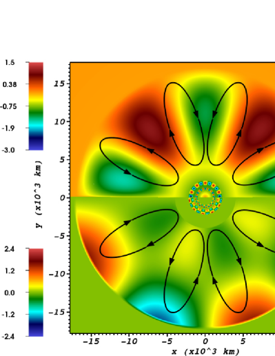
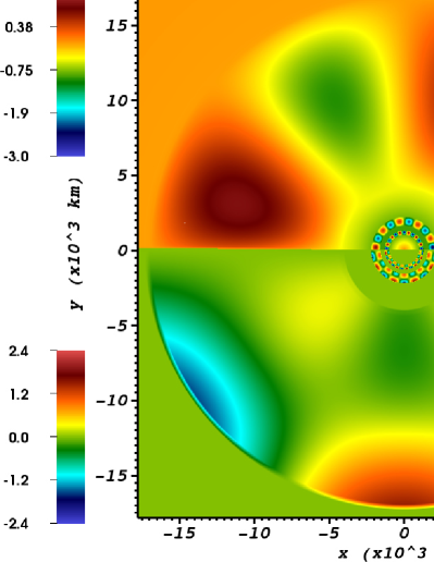
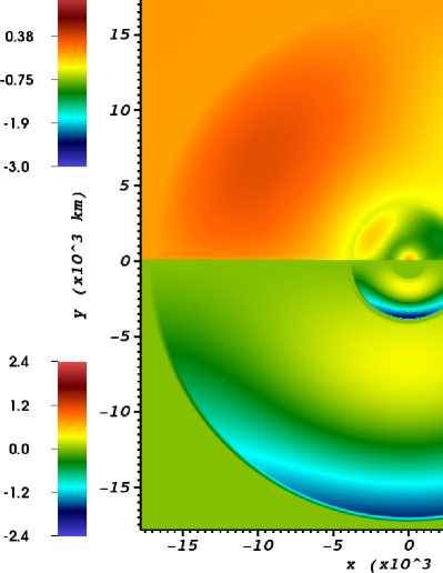
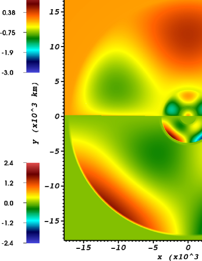
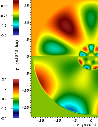
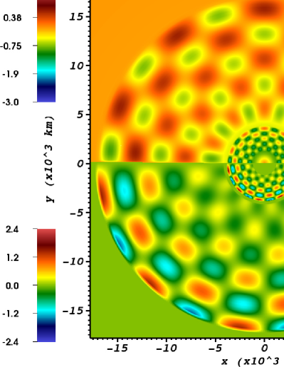
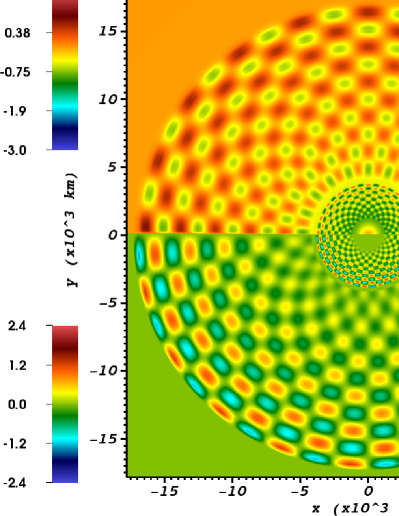
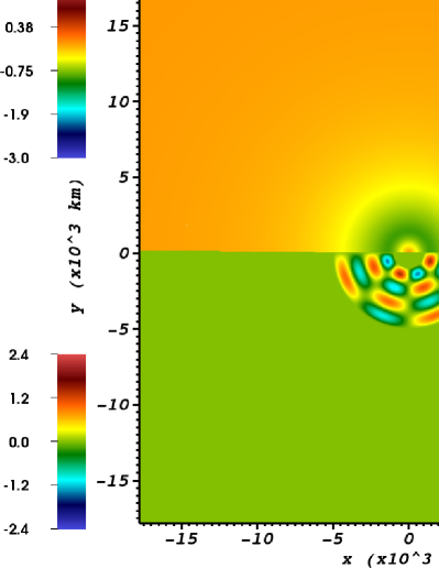
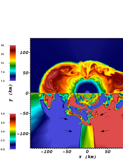
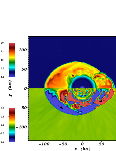
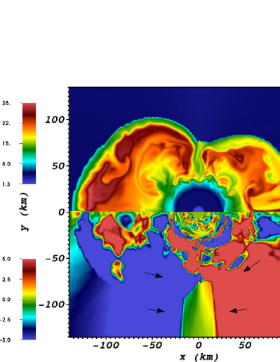
In total, we study ten different perturbation patterns for velocity and density, and consider a number of different amplitudes for each pattern. We refer to the individual models as pXaY, where X denotes the perturbation pattern and Y denotes the amplitude relative to an arbitrarily chosen reference amplitude. The initial configurations for the reference models pXa1 are visualised in Figs. 1 –3. All other models are obtained by rescaling the perturbation amplitude by a factor of $Y$. In the following, we describe the individual perturbation patterns in more detail.

3.1.1 Solenoidal Momentum Density Field (Models pPSaY, pPAaY, pLZaY)

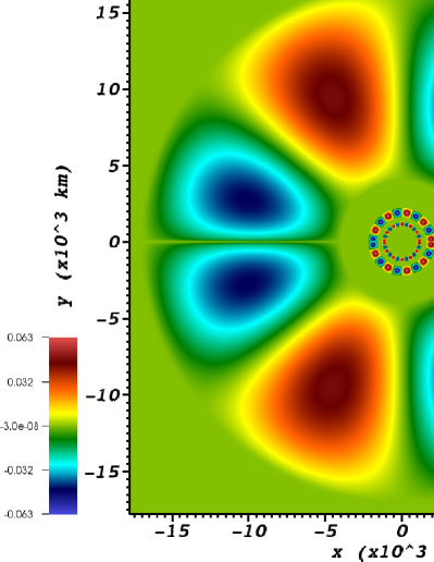
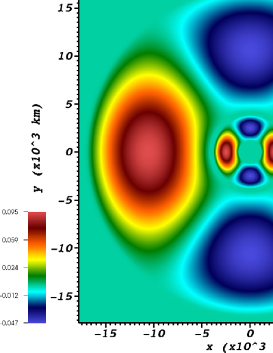
For the majority of our simulations, we consider pure velocity perturbations that obey the divergence-free condition $\nabla\cdot(\rho\mathbf{v})=0$ (Fig. 1 and left panel of Fig. 2). These are generated by expressing the (vectorial) velocity perturbation $\delta\mathbf{v}$ in terms of the curl of a generalised stream function $\boldsymbol{\psi}$,

$$\mathbf{\delta\mathbf{v}}=\left\{\begin{array}[]{ll}\frac{C}{\rho}\nabla\times\boldsymbol{\psi},&r_{\mathrm{min}}\leq r\leq r_{\mathrm{max}}\\ 0,&\ \mathrm{else}\end{array}\right.$$ (6)

where $r_{\mathrm{min}}$ and $r_{\mathrm{max}}$ are the inner and outer boundary of the convective layer. For a single convective layer, we parameterise $\boldsymbol{\psi}$ as

$$\boldsymbol{\psi}=\mathbf{e}_{\varphi}\frac{\sqrt{\sin\theta}}{r}\sin\left(n\pi\frac{r-r_{\mathrm{min}}}{r_{\mathrm{max}}-r_{\mathrm{min}}}\right)Y_{\ell,1}(\theta,0),$$ (7)

where $n$ and $\ell$ denote the number of convective cells in the radial and angular direction, respectively. We use the following definition for the spherical harmonics $Y_{\ell,m}$ for non-negative $m$ in terms of the associated Legendre polynomials $P_{\ell}^{m}$:

$$Y_{\ell,m}(\theta,\varphi)=\sqrt{\frac{2\ell+1}{4\pi}\frac{(\ell-m)!}{(\ell+m)!}}P_{\ell}^{m}(\cos\theta)e^{im\varphi}.$$ (8)

The factor $\sqrt{\sin\theta}$ and the choice of $Y_{\ell,1}$ for the angular dependence of $\boldsymbol{\psi}$ instead of $Y_{\ell,0}$ is critical to avoid singularities at $\theta=0$ and $\theta=\pi$, and also guarantees $\delta v_{\theta}(0)=0$ and $\delta v_{\theta}(\pi)=0$, as well as $\delta v_{r}=0$ at the boundaries of the convective layer (i.e. convective overshoot is not included). Furthermore, this definition ensures that velocity perturbations are isotropic in the sense that the maximum velocities in the convective eddies do not depend on latitude for $\ell\rightarrow\infty$. For a logarithmic density gradient in the progenitor close to $\partial\ln\rho/\partial\ln r\approx-2$ , our prescription also results in roughly constant maximum radial velocities in the case of multiple convective eddies stacked onto each other in a convective shell.

The formalism presented here provides a convenient and simple way to generate solenoidal momentum perturbations with a preferred spatial scale. Capturing the full spectrum of turbulent eddies (with a prescribed power spectrum) is less straightforward. The approach of Chatzopoulos, Graziani & Couch (2014) (decomposition into divergence-free eigenfunctions of the vector Helmholtz equation expressed in terms of vector spherical harmonics) may be better adapted to handle this more general case.

Several distinct convective shells may reach the shock during the first $\mathord{\sim}1\ \mathrm{s}$ of the post-bounce evolution depending on the progenitor structure, and we therefore combine several perturbation patterns computed according to equations (6) and (7) in our models. The different perturbation geometries are summarised in Table 1, and some supplementary information about the relative strength of radial and lateral motions is provided in Table 2.

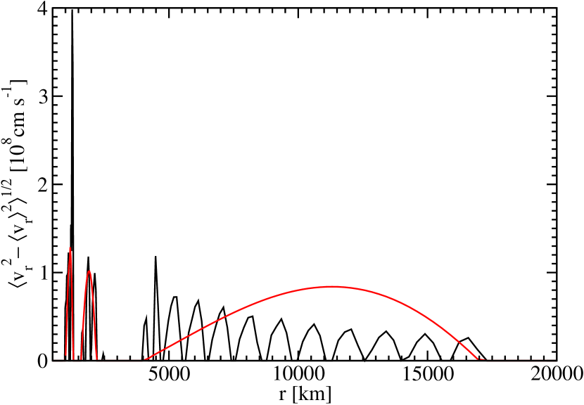
The setup of models pPSa1 and pPAa1 is based on a mixing-length estimate of the unstable regions and the typical convective velocities in the progenitor determined using equation (1), which indicates the existence of two relatively narrow convection zones and a more extended convective layer driven by neon burning. The RMS (root mean square) deviation of the radial velocity $v_{r}$ from its spherical average is compared to the (noisy) mixing-length estimate in Fig. 4; only a rough agreement of the average convective velocities can be reached. The angular wavenumber is chosen such that the angular and radial extent of the convective eddies similar. Model pPSa1 differs from model pPAa1 in that the total momentum of the perturbed configuration vanishes in the former case.

Despite potential numerical problems in discretising equation (1), the location and extent of the unstable regions obtained from equation (1) is roughly compatible with the original stellar evolution calculation in the Kepler code (Woosley & Heger, 2007). The region between $1000\ \mathrm{km}$ and $1300\ \mathrm{km}$ is not Ledoux-unstable in the original stellar evolution model (except for a single zone flagged as convective), but there is a thermohaline convection layer between $900\ \mathrm{km}$ and $1500\ \mathrm{km}$. Convective instability is indicated for $1500\ \mathrm{km}\leq r<2300\mathrm{km}$ and $3900\ \mathrm{km}\leq r\leq 18000\ \mathrm{km}$, i.e. these convective zone are only a little wider in Kepler than predicted by our post-processing approach. Thus, even a naive, straightforward discretisation of equation (1) seems to yield acceptable predictions for convective instability.

The pLZ models (where Z denotes the angular wavenumber) are geared towards a more systematic exploration of possible flow geometries. For these models, we assume a wide convective layer encompassing both the Si and Si/O shells and another convective zone in the O/Ne/Mg shell. We vary the scale of the convective eddies, covering angular wavenumbers from $\ell=1$ to $\ell=20$, as well as the amplitude of the velocity perturbation $\mathbf{\delta v}$. To a lesser extent, these variations in flow geometry are motivated by the possibility that strong shell interactions (Arnett & Meakin, 2011) could lead to a merger of different convection zones, which is one among many uncertainties in the structure of pre-supernova cores. A more important reason, however, lies in the fact that the extent of the convective shells varies greatly between progenitor models (see again the Kippenhahn diagrams in Heger, Langer & Woosley 2000)

The pLZ perturbations are also set up such that the convective eddies are of similar extent in the radial and lateral direction, but because of the broader “convection zones” this cannot be perfectly accomplished for $\ell=1,2$ and only only for a restricted range in radius for large $\ell>4$ with our functional ansatz for the generalised stream function. As a result, there is some variation in the relative strength of radial and lateral motions (see Table 2), and some perturbation patterns do not conform to the expectation (Arnett, Meakin & Young, 2009) of equipartition between the kinetic energy in radial motions and the combined energy in transverse motions in all other directions (which, however, need not be universally valid).

3.1.2 Purely Transverse Velocity Perturbations (Models pCOaY)

In addition, we also study a perturbation pattern similar to the one used by Couch & Ott (2013) (right panel of Fig. 2). Different from Couch & Ott (2013), the perturbation pattern pCO is axisymmetric; it is essentially a meridional cut through their model n5m2 that we revolve around the symmetry axis of the spherical polar grid. Furthermore, we perturb the initial model at the onset of collapse whereas Couch & Ott (2013) imposed perturbations at bounce. Only the lateral velocity component $v_{\theta}$ is perturbed. For model pCOaX, $v_{\theta}$ is given by

$$v_{\theta}=0.2\times c_{s}\sin\left(4\theta\right)\sin\left(4\pi\frac{r-1000\ \mathrm{km}}{4000\ \mathrm{km}}\right),$$ (9)

in terms of the local sound speed $c_{s}$ for $1000\ \mathrm{km}\leq r\leq 4000\ \mathrm{km}$.

It must be emphasised that this perturbation pattern hardly resembles a convective flow. The radial velocity field is spherically symmetric, i.e. convective updrafts and downdrafts are absent. The velocity field also violates the divergence-free condition. This results in a strong (and probably unphysical) excitation of acoustic waves in the perturbed (and supposedly “convective”) region as the model evolves. We nevertheless include this perturbation pattern in our model suite as the closest possible analogue to the models of Couch & Ott (2013) in 2D.

3.1.3 Density Perturbations (Models pPDaY and pDL2aY)

In addition to velocity perturbations, we also explore a smaller set of models with density perturbations (Fig. 3). We confine ourselves to one series (pPD) where the convective regions are estimated using equation (2) for the mixing-length density contrast and to a series (pDL2) with two large convective zones and large-scale $\ell=2$ density perturbations. Within each zone, the density contrast is calculated as follows,

$$\frac{\delta\rho}{\rho}=D\sin\left(n\pi\frac{r-r_{\mathrm{min}}}{r_{\mathrm{max}}-r_{\mathrm{min}}}\right)Y_{\ell,0}(\theta,0),\quad\mathrm{for}\ r_{\mathrm{min}}\leq r\leq r_{\mathrm{max}}.$$ (10)

The values for $D$, $r_{\mathrm{min}}$, $r_{\mathrm{max}}$, and $\ell$ for the individual zones are shown in Table 3. Note that we also include one model (pPDLa2m) with a negative value for the normalised perturbation amplitude, i.e. the maxima and minima of the density perturbation $\delta\rho$ are interchanged in this model compared to model pPDLa2.

Figure 4: RMS deviation $\delta v=\sqrt{\langle v_{r}^{2}-\langle v_{r}^{2}\rangle\rangle}$ of the radial velocity $v_{r}$ from its angular average for perturbation pattern pPSa1 (red line) compared to a mixing-length estimate (black) computed from the progenitor profile using equation (1).

Table 4: Simulation Results – Velocity Perturbations

perturbation	$v_{\theta,\mathrm{max}}$	$\mathrm{Ma}_{\theta,\mathrm{max}}$	$E_{\mathrm{kin},\theta,\mathrm{ini}}$	$\zeta$	comment	explosion	$\mathrm{Ma}_{\theta,\mathrm{expl}}$
pattern	$(10^{8}\ \mathrm{cm}\ \mathrm{s}^{-1})$		$(10^{48}\ \mathrm{erg})$			time
p0	0	0	0	0	unperturbed baseline model	—	—
pPSa1	$2.37$	$0.59$	$2.78$	$0.9\%$	Ledoux-unstable zones, symmetric	—	—
pPSa2	$4.74$	$1.19$	$11.2$	$3.5\%$	Ledoux-unstable zones, symmetric	$680\ \mathrm{ms}$	$0.07$
pPSa4	$9.49$	$2.37$	$44.6$	$14\%$	Ledoux-unstable zones, symmetric	—	—
pPAa1	$2.37$	$0.58$	$2.83$	$0.9\%$	Ledoux-unstable zones, asymmetric	—	—
pPAa2	$4.74$	$1.16$	$11.3$	$3.5\%$	Ledoux-unstable zones, asymmetric	$820\ \mathrm{ms}$	$0.08$
pPAa4	$9.49$	$2.32$	$45.2$	$14\%$	Ledoux-unstable zones, asymmetric	$830\ \mathrm{ms}$	$0.16$
pL1a0.25	$0.45$	$0.16$	$0.19$	$0.06\%$	two large zones, $\ell=1$	—	—
pL1a0.5	$0.89$	$0.32$	$0.75$	$0.23\%$	two large zones, $\ell=1$	$810\ \mathrm{ms}$	$0.19$
pL1a1	$1.78$	$0.63$	$3.00$	$0.9\%$	two large zones, $\ell=1$	$530\ \mathrm{ms}$	$0.25$
pL1a2	$3.56$	$1.26$	$12.0$	$3.8\%$	two large zones, $\ell=1$	$480\ \mathrm{ms}$	$0.35$
pL2a0.0625	$0.11$	$0.04$	$0.01$	$0.003\%$	two large zones, $\ell=2$	—	—
pL2a0.125	$0.21$	$0.08$	$0.04$	$0.01\%$	two large zones, $\ell=2$	$750\ \mathrm{ms}$	$0.05$
pL2a0.25	$0.43$	$0.15$	$0.16$	$0.05\%$	two large zones, $\ell=2$	$740\ \mathrm{ms}$	$0.09$
pL2a0.5	$0.86$	$0.30$	$0.62$	$0.19\%$	two large zones, $\ell=2$	$720\ \mathrm{ms}$	$0.18$
pL2a1	$1.72$	$0.61$	$2.50$	$0.79\%$	two large zones, $\ell=2$	$480\ \mathrm{ms}$	$0.20$
pL2a2	$3.43$	$1.22$	$10.0$	$3.1\%$	two large zones, $\ell=2$	$420\ \mathrm{ms}$	$0.25$
pL2a4	$6.87$	$2.43$	$40.0$	$13\%$	two large zones, $\ell=2$	$300\ \mathrm{ms}$	$0.20$
pL4a0.5	$0.85$	$0.30$	$0.57$	$0.18\%$	two large zones, $\ell=4$	—	—
pL4a1	$1.70$	$0.60$	$2.29$	$0.72\%$	two large zones, $\ell=4$	$700\ \mathrm{ms}$	$0.35$
pL4a2	$3.40$	$1.20$	$9.2$	$2.9\%$	two large zones, $\ell=4$	$480\ \mathrm{ms}$	$0.35$
pL4a4	$6.81$	$2.41$	$36.6$	$11\%$	two large zones, $\ell=4$	$290\ \mathrm{ms}$	$0.20$
pL10a1	$0.82$	$0.29$	$0.47$	$0.15\%$	two large zones, $\ell=10$	—	—
pL10a1	$1.63$	$0.58$	$1.87$	$0.58\%$	two large zones, $\ell=10$	$790\ \mathrm{ms}$	$0.35$
pL10a2	$3.27$	$1.16$	$7.49$	$2.3\%$	two large zones, $\ell=10$	$800\ \mathrm{ms}$	$0.70$
pL10a4	$6.54$	$2.32$	$30.0$	$9.4\%$	two large zones, $\ell=10$	$510\ \mathrm{ms}$	$1.00$
pL20a0.5	$0.73$	$0.26$	$0.40$	$0.13\%$	two large zones, $\ell=20$	—	—
pL20a1	$1.45$	$0.52$	$1.61$	$0.5\%$	two large zones, $\ell=20$	$710\ \mathrm{ms}$	$0.30$
pL20a2	$2.90$	$1.04$	$6.42$	$2.0\%$	two large zones, $\ell=20$	$740\ \mathrm{ms}$	$0.60$
pL20a4	$5.81$	$2.07$	$25.7$	$8.0\%$	two large zones, $\ell=20$	$560\ \mathrm{ms}$	$0.80$
pCOa0.25	$0.35$	$0.05$	$0.13$	$0.02\%$	transverse velocity perturbations	$800\ \mathrm{ms}$	$0.05$
pCOa0.5	$0.69$	$0.10$	$0.53$	$0.08\%$	transverse velocity perturbations	$700\ \mathrm{ms}$	$0.10$
pCOa1	$1.39$	$0.20$	$2.14$	$0.34\%$	transverse velocity perturbations	$650\ \mathrm{ms}$	$0.20$
pCOa2	$2.77$	$0.40$	$8.55$	$1.36\%$	transverse velocity perturbations	$270\ \mathrm{ms}$	$0.40$
pCOa4	$5.55$	$0.80$	$34.3$	$5.4\%$	transverse velocity perturbations	$240\ \mathrm{ms}$	$0.80$

$v_{\theta,\mathrm{max}}$ is the maximum absolute value of the $\theta$-component of the perturbation velocity, $\mathrm{Ma}_{\theta,\mathrm{max}}$ is the Mach number corresponding to this velocity, $E_{\mathrm{kin},\theta,\mathrm{ini}}$ is the lateral kinetic energy contained in the velocity perturbations, $\zeta$ is the ratio of this energy to the binding energy of the perturbed mass shells, and $\mathrm{Ma}_{\theta,\mathrm{expl}}$ is the maximum lateral Mach number in the initial model inside the mass shell that reaches the shock at the onset of the explosion.

Table 5: Simulation Results – Density Perturbations

perturbation			explosion
pattern	$(\delta\rho/\rho)_{\mathrm{max}}$	comment	time
pPDa1	$0.07$	Ledoux-unstable zones	—
pPDa2	$0.13$	Ledoux-unstable zones	$880\ \mathrm{ms}$
pPDa4	$0.25$	Ledoux-unstable zones	$880\ \mathrm{ms}$
pDL2a1	$0.09$	two large zones, $\ell=2$	$780\ \mathrm{ms}$
pDL2a2	$0.18$	two large zones, $\ell=2$	$710\ \mathrm{ms}$
pDL2a4	$0.36$	two large zones, $\ell=2$	$630\ \mathrm{ms}$
pDL2a2m	$0.18$	two large zones, $\ell=2$	—

$(\delta\rho/\rho)_{\mathrm{max}}$ is the maximum relative deviation of the density from its spherical average in the initial model.

3.2 Numerical Methods

We evolve the perturbed progenitor models as well as an unperturbed baseline model (p0) with very small inherent numerical seed perturbations from the onset of collapse to at least $800\ \mathrm{ms}$ after bounce using the relativistic hydrodynamics code CoCoNuT (Dimmelmeier, Font & Müller, 2002). During the collapse, we apply the deleptonisation scheme of Liebendörfer (2005). At bounce, we switch to a newly developed fast multi-group neutrino transport (FMT) scheme based on an approximate solution of the neutrino energy equation. The required closure relation is provided by solving the Boltzmann equation in a two-stream approximation (which yields an accurate flux factor at high optical depths). At larger distances from the neutrinosphere, we match to a solution for the flux factor derived from an analytic variable Eddington factor closure. We take all the relevant charged-current reactions as well as isoenergetic neutral-current neutrino interactions with nucleons and nuclei into account (see Appendix A for details). Furthermore, we include an effective one-particle rate for nucleon-nucleon bremsstrahlung and approximately account for the energy exchange of $\mu$ and $\tau$ neutrinos with the medium due to nucleon recoil in neutral-current scattering. A comparison with results from the Vertex-Prometheus code and its relativistic offshoot Vertex-CoCoNuT shows that our new scheme allows us to achieve reasonable qualitative and quantitative agreement with more sophisticated methods for multi-group neutrino transport at a fraction of the computational cost. For a detailed description of the neutrino transport treatment in our simulations, we refer the reader to Appendix A.

However, future users of our method should bear in mind that these savings come at a cost, and one must check the approximations inherent in the FMT scheme on a case-by-case basis: We already mentioned the limitations of the FMT scheme during the collapse phase (where neutrino-electron scattering cannot be neglected). Moreover, many of the complexities of neutrino-nucleon interactions at high densities are presently ignored, such as nucleon correlations (Burrows & Sawyer, 1998, 1999; Reddy et al., 1999), the effect of nucleon interaction potentials (Martínez-Pinedo et al., 2012; Roberts, Reddy & Shen, 2012), weak magnetism (Horowitz, 1997), and the quenching of the axial-vector coupling at high densities (Carter & Prakash, 2002). This would, among other things, delay the cooling of the proto-neutron star considerably (Hüdepohl et al., 2009), and could affect the nucleosynthesis conditions after the onset of the explosion, which are very sensitive to the difference of the electron neutrino and anti-neutrino luminosities and mean energies. As with any transport scheme (flux-limited diffusion, the IDSA approximation of Liebendörfer, Whitehouse & Fischer 2009, or even two-moment closure schemes) not based on a rigorous solution of the Boltzmann equation or a Boltzmann closure, the flux factor at intermediate optical depths $\lesssim 1$ (which is crucial for the neutrino heating and cooling) requires careful checking.

We use a computational grid with $N_{r}\times N_{\theta}=550\times 256$ zones to cover the innermost $10^{5}\ \mathrm{km}$ of the progenitor. In the innermost $10\mathrm{km}$, the grid spacing is fairly uniform and then transitions smoothly to a roughly logarithmic grid spacing with $\Delta r/r\approx 1.5\%$ between $10\ \mathrm{km}$ and $400\ \mathrm{km}$. Outside $400\ \mathrm{km}$, $\Delta r/r$ gradually rises to $2.2\%$ at the outer boundary. An equidistant grid is used for the $\theta$-coordinate.

For the high-density regime, we employ the equation of state of Lattimer & Swesty (1991) with a bulk incompressibility modulus of nuclear matter of $K=220\ \mathrm{MeV}$ (LS220). At densities lower than $5\times 10^{8}\ \mathrm{g}\ \mathrm{cm}^{-3}$ (prior to bounce) or $10^{11}\ \mathrm{g}\ \mathrm{cm}^{-3}$ (after bounce), we include the ideal gas contributions of photons, electrons/positrons of arbitrary degeneracy, and of 17 different nuclear species (protons, neutrons, $\alpha$-particles, and 14 intermediate and heavy nuclei). Nuclear burning is taken into account nuclear burning according to the “flashing” treatment of Appendix B.2 in Rampp & Janka (2002). Above a temperature of $T=0.5\ \mathrm{MeV}$, we switch to nuclear statistical equilibrium.

4 Overview of Simulation Results

Our simulations show that sufficiently strong asphericities in the progenitor can indeed tip the scales in favour of an explosion for a rather pessimistic model. While the shock is not revived in the baseline model p0 at least until $1.4\ \mathrm{s}$ after bounce, an explosion develops in many of the simulations with initial perturbations. The final fate of the different models is summarised in the penultimate of Tables 4 (velocity perturbations) and 5 (density perturbations).

These tables give the time of explosion for each model (if applicable), which we define as the time when the critical ratio between the advection time-scale and the heating time-scale (defined as in Müller, Janka & Marek 2012) reaches unity. For the models with velocity perturbations, we also list the maximum lateral velocity $v_{\theta,\mathrm{max}}$, the maximum Mach number $\mathrm{Ma}_{\theta,\mathrm{max}}$ corresponding to this velocity, and the total kinetic energy $E_{\mathrm{kin},\theta,\mathrm{ini}}$ contained in lateral motions in the initial model. The ratio $\zeta$ of this energy to the total binding energy (i.e. gravitational energy + internal energy) of the perturbed mass shells is also provided. Since the lateral Mach number varies considerably with radius in the models with solenoidal perturbations, we also give the maximum lateral Mach number $\mathrm{Ma}_{\theta,\mathrm{expl}}$ in the initial model inside the mass shell that reaches the shock at the time of the explosion. This number provides a better measure for the violence of convective motions in the progenitor that is required to achieve shock revival. For models with density perturbations, we provide the maximum of $\delta\rho/\rho$ in the initial model. When comparing to multi-D stellar evolution models or mixing-length estimates, the reader should always carefully consider whether average or maximum quantities are involved.

The numbers in these tables suggest some systematic trends, but also show the dependence on the perturbation pattern and amplitude to be non-trivial in some cases.

Perturbations restricted to regions where we diagnose convective instability in the progenitor models based on the Ledoux criterion appear to be relatively inefficient at boosting the heating conditions. For the model series pPAaX and pPSaX with velocity perturbations, we only obtain explosions for $E_{\mathrm{kin},\theta,\mathrm{ini}}>1.1\times 10^{49}\mathrm{erg}$, and the strongly perturbed model pPSa4 even fails to explode. Shock revival does not occur earlier than $680\ \mathrm{ms}$ after bounce (model pPSa2).

Explosions occur more readily in models with perturbations in the entire silicon and oxygen shells, or with the perturbation pattern pCOaX inspired by the setup of Couch & Ott (2013). Low-$\ell$ perturbations with $\ell=2$ and $\ell=1$ emerge as most efficient in inducing an explosion, which can occur around $500\ \mathrm{ms}$ with reasonably subsonic velocity ($\mathrm{Ma}_{\theta,\mathrm{expl}}\leq 0.25$ for these cases). Perturbations with higher $\ell$ tend to be less effective for a given maximum Mach number, but there are exceptions as models pL20a1 and pL20a2 explode earlier than models pL10a1 and pL10a2. Larger perturbations generally result in earlier explosions, but there are also some non-monotonicities (pL10a2 explodes later than pL10a1 and pL20a2 explodes later than pL20a1).

The non-solenoidal perturbation pattern pCOaX mimicking the setup of Couch & Ott (2013) in 2D tends to give earlier explosions for a given value of $\mathrm{Ma}_{\theta,\mathrm{max}}$ or $E_{\mathrm{kin},\theta,\mathrm{ini}}$ than the corresponding solenoidal perturbation pattern with $\ell=4$. The earliest explosions are found for this perturbation pattern with large initial amplitudes ($E_{\mathrm{kin},\theta,\mathrm{ini}}$ up to $3.4\times 10^{49}\ \mathrm{erg}$).

Density perturbations in the progenitor likewise lead to shock revival in some cases, but rather high perturbation amplitudes are required to achieve explosions as early as for velocity perturbations with low $\ell$. We find an appreciable effect only if the density contrast is of the order of $\delta\rho/\rho\approx 0.1$, which would require a convective Mach number of $\mathrm{Ma}_{\mathrm{prog}}\gtrsim 0.3$ in the O-burning shell.

Figure 5: Top: Time evolution of the maximum (black solid curve), average (black, dashed), and minimum (black, solid) shock radius for the baseline model p0. The proto-neutron star radius (red), defined by a fiducial density of $10^{11}\ \mathrm{g}\ \mathrm{cm}^{-3}$, the gain radius (black, dotted), and the mass accretion rate $\dot{M}$ (measured at a radius of $400\ \mathrm{km}$, blue, dash-dotted, scale on the right vertical axis) are also shown. Bottom: Coefficients $a_{1}$ (black) and $a_{2}$ (red) for the decomposition of the shock surface into Legendre polynomials.

Figure 6: Total neutrino luminosities (top panel) and angle-averaged mean energies (bottom panel) for the baseline model p0. Black, red, and blue curves are used for $\nu_{e}$, $\bar{\nu}_{e}$, and $\nu_{\mu/\tau}$, respectively. All quantities are measured at a radius of $400\ \mathrm{km}$.

Figure 7: Time-scale criterion $\tau_{\mathrm{adv}}/\tau_{\mathrm{heat}}$ (black), volume-integrated neutrino heating rate in the gain region (red), and heating efficiency $\eta$ (blue) for the baseline model p0.

Figure 8: Approach of the baseline model to the critical curve in the $(M\dot{M},L_{\nu}E_{\nu}^{2})$ plane (see Section 5.3). Here, $L_{\nu}$ is the total electron flavor luminosity, and $E_{\nu}$ is an appropriate average of electron neutrino and anti-neutrino mean energies (equation 14). The black curve shows the evolution of the model (with red circles indicating its state at four selected post-bounce times), and a fiducial critical curve (dashed) is anchored at the final location of the model in the $(M\dot{M},L_{\nu}E_{\nu}^{2})$-plane where the time-scale ratio $\tau_{\mathrm{adv}}/\tau_{\mathrm{heat}}$ approaches unity. The blue circle roughly indicates the time when the neon burning shell reaches the shock.

Figure 9: Comparison of the evolution of the total electron flavour luminosity (black) with the prediction of equation (16) of Pejcha & Thompson (2012, PT2012 for short) for the critical luminosity (red). Note that this estimate for the critical luminosity increases with time instead of decreasing, thus erroneously suggesting a deterioration in heating conditions for model p0. A modified version of equation (16) of PT2012 that includes a correction term $\propto E_{\bar{\nu}_{e}}^{-2}$ (O. Pejcha, private communication) is also shown in blue; it still does not give the expected decrease.

5 Heating Conditions and Multi-Dimensional Instabilities in the Baseline Model

In order to provide the required background for interpreting the evolution of the perturbed models, we first analyse the baseline model p0 in some detail. In particular, we introduce the concept of the critical neutrino luminosity (Burrows & Goshy, 1993) in a form best suited for our further analysis (Section 5.3). We also define quantities needed later for comparing perturbed and unperturbed models, and collect several useful scaling relations connecting the heating conditions and the activity of non-radial hydrodynamic instabilities (Section 5.4).

5.1 Shock Evolution

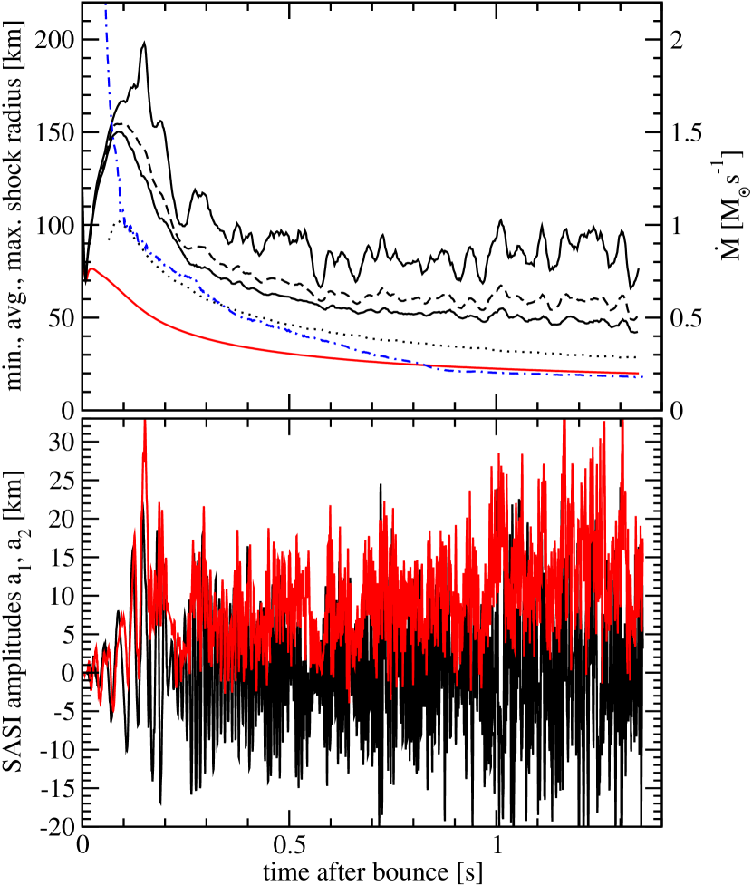
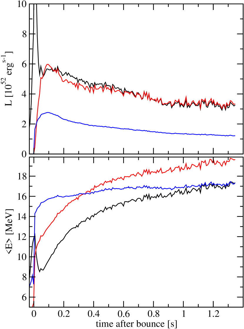
Figs. 5–7 provide a compact overview of the evolution of the baseline model p0. The shock trajectories, the evolution of non-radial shock oscillations, the contraction of the proto-neutron star, the neutrino emission, and the flow morphology are all in good qualitative and quantitative agreement with recent 2D simulations based on more ambitious multi-group neutrino transport methods.

The top panel of Fig. 5 shows the maximum, minimum, and average shock radii ($r_{\mathrm{sh,min}}$, $r_{\mathrm{sh,min}}$ and $r_{\mathrm{sh}}$) along with the gain radius and proto-neutron star radius. The average shock radius reaches a maximum value of $\approx 150\ \mathrm{km}$ at a time of $100\ \mathrm{ms}$ after bounce and steadily recedes thereafter, following the contraction of the proto-neutron star. From around $100\ \mathrm{ms}$, multi-dimensional instabilities lead to a sizeable deformation of the shock. This is also reflected by the Legendre coefficients $a_{1}$ and $a_{2}$ for the dipole and quadrupole deformation of the shock (bottom panel of Fig. 5). We define $a_{\ell}$ in terms of the $\ell$-th Legendre polynomial $P_{\ell}$ and the angle-dependent shock radius $r_{\mathrm{sh}}(\theta)$ as

$$a_{\ell}=\frac{2\ell+1}{2}\int\limits_{0}^{\pi}r_{\mathrm{sh}}(\theta)P_{\ell}(\cos\theta)\,\mathrm{d}\cos\theta.$$ (11)

We also use $a_{0}$ as the average shock radius $r_{\mathrm{sh}}$ in Fig. 5. The dipole and quadrupole amplitudes are typically in the range of $10\ldots 20\ \mathrm{km}$ throughout the simulation. It is noteworthy that $a_{2}$ is almost invariably positive, i.e. the shock always exhibits a prolate deformation.

5.2 Neutrino Emission

The neutrino luminosities and mean energies (Fig. 6) likewise show a familiar picture. There is a steady and very gradual decline of the luminosity of all flavors from $100\ \mathrm{ms}$ after bounce onward. The mean energies rise steadily with a crossing of $\bar{\nu}_{e}$ and $\nu_{\mu/\tau}$ energies around $0.3\ \mathrm{ms}$ that is well known for more massive progenitors (Müller & Janka, 2014; Marek, Janka & Müller, 2009). At very late times (around $1.3\ \mathrm{s}$), there is even another crossing of electron neutrino and heavy flavor neutrino mean energies due to the “accretion effect” identified by Müller & Janka (2014) (i.e. a temperature inversion develops in the accretion layer around the neutrinosphere so that the effective temperature of the heavy flavor neutrinos originating from deeper layers drops below that of the electron flavour neutrinos and anti-neutrinos).

5.3 Secular Evolution of the Heating Conditions and Approach to the Critical Luminosity

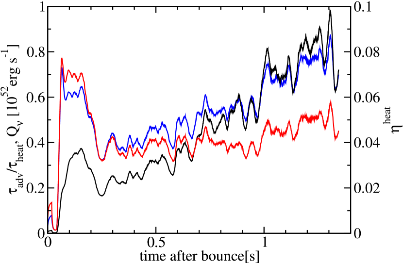
Fig. 7 shows the critical ratio of the advection and heating time-scales $\tau_{\mathrm{adv}}$ and $\tau_{\mathrm{heat}}$ (defined as in Müller, Janka & Marek 2012), the volume-integrated neutrino heating rate $\dot{Q}_{\nu}$ in the gain region, and the heating efficiency $\eta_{\mathrm{heat}}$ (defined as the ratio between $\dot{Q}_{\nu}$ and the sum of the electron flavor luminosities $L_{\nu_{e}}+L_{\bar{\nu}_{e}}$). The critical time-scale ratio $\tau_{\mathrm{adv}}/\tau_{\mathrm{heat}}$ remains below unity throughout the entire simulation. During the first second it never exceeds $0.6$, which indicates that the model is indeed relatively far from an explosive runaway. However, $\tau_{\mathrm{adv}}/\tau_{\mathrm{heat}}$ comes close to the critical threshold towards the very end of the simulation. We likewise observe a slow increase of $\eta_{\mathrm{heat}}$ after some $250\ \mathrm{ms}$. The volume-integrated heating rate remains high ($\approx 4\times 10^{51}\ \mathrm{erg}\ \mathrm{s}^{-1}$) at late times, and also exhibits a slight secular increase.

As shown by Janka (2012), the time-scale criterion $\tau_{\mathrm{adv}}/\tau_{\mathrm{heat}}\gtrsim 1$ can be re-formulated as a condition for the “critical luminosity” (Burrows & Goshy, 1993; Murphy & Burrows, 2008; Pejcha & Thompson, 2012) required for a successful explosion for a given mass accretion rate $\dot{M}$. This perspective will be useful for understanding why the baseline model p0 as well as other general relativistic and pseudo-relativistic models with ray-by-ray variable Eddington factor transport (Marek & Janka, 2009; Müller, Janka & Marek, 2012) show a secular increase of the time-scale ratio $\tau_{\mathrm{adv}}/\tau_{\mathrm{heat}}$ at late times.

For estimating the critical luminosity, we note that $\tau_{\mathrm{adv}}$ scales roughly as (Janka, 2012),

$$\tau_{\mathrm{adv}}\propto\frac{r_{\mathrm{sh}}^{3/2}}{\sqrt{M}},$$ (12)

where $r_{\mathrm{sh}}$ can in turn be expressed in terms of the total electron flavor luminosity $L_{\nu}=L_{\nu_{e}}+L_{\bar{\nu}_{e}}$, the mean energy $E_{\nu}$ of electron neutrinos and anti-neutrinos, the gain radius $r_{\mathrm{gain}}$, the mass accretion rate $\dot{M}$, and the proto-neutron star mass $M$ as (see Janka 2012 and Appendix B)

$$r_{\mathrm{sh}}\propto\frac{(L_{\nu}E_{\nu}^{2})^{4/9}r_{\mathrm{gain}}^{16/9}}{\dot{M}^{2/3}M^{1/3}}.$$ (13)

Here $E_{\nu}$ is defined as a weighted average of electron neutrino and anti-neutrino mean energies:

$$E_{\nu}^{2}=\frac{L_{\nu_{e}}E_{\nu_{e}}^{2}+L_{\bar{\nu}_{e}}E_{\bar{\nu}_{e}}^{2}}{L_{\nu_{e}}+L_{\bar{\nu}_{e}}}.$$ (14)

The heating time-scale can be expressed in terms of the mass in the gain region $M_{\mathrm{gain}}$, the average mass-specific binding energy $|e_{\mathrm{gain}}|$, the neutrino luminosity $L_{\nu}$, and the heating efficiency $\eta_{\mathrm{heat}}$ as

$$\tau_{\mathrm{heat}}\approx\frac{M_{\mathrm{gain}}|e_{\mathrm{gain}}|}{L_{\nu}\eta_{\mathrm{heat}}}.$$ (15)

Since

$$\eta_{\mathrm{heat}}\propto\frac{M_{\mathrm{gain}}E_{\nu}^{2}}{r_{\mathrm{gain}}^{2}}$$ (16)

holds to very good approximation (Janka, 2012), this implies

$$\tau_{\mathrm{heat}}\propto\frac{|e_{\mathrm{gain}}|r_{\mathrm{gain}}^{2}}{L_{\nu}E_{\nu}^{2}}.$$ (17)

While Janka (2012) posits that $|e_{\mathrm{gain}}|$ scales with the gravitational potential $GM/r_{\mathrm{gain}}$ at the gain radius, simply using either the gravitational potential energy or the internal energy to determine the heating time-scale may introduce uncertainties on the level of a few tens of percent in the critical threshold (Murphy & Burrows, 2008; Pejcha & Thompson, 2012). However, the time-scale criterion becomes a very accurate tracer for the runaway threshold if the actual binding energy, i.e. the difference of the internal+kinetic energy and the potential energy, is used (Fernández, 2012). Estimating this difference analytically is not straightforward, but simulations show that the assumption of a time-independent binding energy per baryon actually works rather well. This leads to

$$\tau_{\mathrm{heat}}\propto\frac{r_{\mathrm{gain}}^{2}}{L_{\nu}E_{\nu}^{2}}.$$ (18)

Using these approximate scaling relations, the time-scale criterion $\tau_{\mathrm{adv}}/\tau_{\mathrm{heat}}\sim 1$ then translates into a critical condition for $L_{\nu}E_{\nu}^{2}$ as a function of $\dot{M}$, $M$, and $r_{\mathrm{gain}}$ (which is mostly determined by $M$ through the mass-radius relation for hot neutron stars),

$$(L_{\nu}E_{\nu}^{2})_{\mathrm{crit}}\propto\left(\dot{M}M\right)^{3/5}r_{\mathrm{gain}}^{-2/5}.$$ (19)

Note that unlike Janka (2012) we do not eliminate the gain radius $r_{\mathrm{gain}}$ and the neutrino mean energy $E_{\nu}$ from this relation.

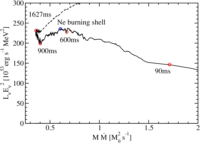
Fig. 8 shows the evolution of $L_{\nu}E_{\nu}^{2}$ versus $\dot{M}M$ along with a critical curve given by equation (19) anchored at a point towards the end of the simulation where $\tau_{\mathrm{adv}}/\tau_{\mathrm{heat}}$ approaches unity. For about $800\ \mathrm{ms}$, the model continuously approaches the critical curve. At this junction, the accretion rate drops slightly as the Neon burning shell reaches the shock and then transitions into a more shallow decline ($\dot{M}\propto t^{-1/3}$ as opposed to $\dot{M}\propto t^{-1}$) at earlier times, reflecting the changing density gradient in the progenitor. For a while, the model then moves parallel to the critical curve, and again starts to approach it around $1\ \mathrm{s}$.

Equation (19) nicely shows the underlying reason for the secular approach to the critical curve, i.e. the increase of the ratio

$$\frac{L_{\nu}E_{\nu}^{2}}{(L_{\nu}E_{\nu}^{2})_{\mathrm{crit}}}\propto\frac{L_{\nu}E_{\nu}^{2}r_{\mathrm{gain}}^{2/5}}{(\dot{M}M)^{3/5}},$$ (20)

and illustrates that it is potentially dangerous to reduce the critical condition to a power law for $L_{\mathrm{crit}}$ in terms of $\dot{M}$ and $M$, or even $\dot{M}$ alone as in the classical form $L_{\mathrm{crit}}=L_{\mathrm{crit}}(\dot{M})$. If we consider the individual quantities ($L_{\nu}$, $E_{\nu}$, $M$, $\dot{M}$, $r_{\mathrm{gain}}$) that enter into the critical condition, we find that the ratio $L_{\nu}/\dot{M}^{3/5}$ becoming more favorable at late times as both the electron flavor luminosity $L_{\nu}$ and the accretion rate $\dot{M}$ decrease. However, the contraction of the proto-neutron star and its growing mass also enter into the critical curve, and, somewhat astonishingly, the ratio $L_{\nu}r_{\mathrm{gain}}^{2/5}/(\dot{M}M)^{3/5}$ is almost constant in model p0 from $\mathord{\sim}100\ \mathrm{ms}$ after bounce. The approach towards the critical curve therefore hinges solely on the secular increase of the neutrino mean energy ($E_{\nu}\propto M$, see Müller & Janka 2014). While the interplay of the different terms may be somewhat sensitive to the detailed treatment of the neutrino transport, the neutrino opacities, and the equation of state, this suggests that at least for massive progenitors without an early and abrupt drop of the mass accretion rate, this highlights the paramount importance of the mean energies for an explosive runaway due to neutrino heating.

As an aside, we note that the phenomenological scaling relations describing the 2D simulations result in somewhat different power-law exponents for the scaling of the critical luminosity than in the power-law fits of Pejcha & Thompson (2012), who also include the dependence on neutron star mass and radius (in their case, more, precisely the neutrinosphere radius) in equation (16) of their paper: They obtain

$$L_{\nu,\mathrm{core}}^{\mathrm{crit}}=8.18\times 10^{52}\ \mathrm{erg}\ \mathrm{s}^{-1}\times\tau_{\nu}^{-0.206}\left(\frac{M}{M_{\odot}}\right)^{1.84}\left(\frac{\dot{M}}{M_{\odot}\ \mathrm{s}^{-1}}\right)^{0.723}\left(\frac{r_{\nu}}{10\ \mathrm{km}}\right)^{-1.61}$$ (21)

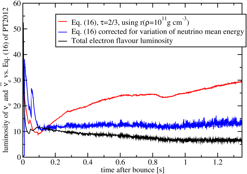
for the critical core luminosity of electron neutrinos and antineutrinos in terms of $M$, $\dot{M}$, and the optical depth $\tau_{\nu}$ and radius $r_{\nu}$ of the neutrinosphere. The dependence on $M$ and $r_{\nu}$ is noticeably steeper than in equation (19). Using $\tau_{\nu}=2/3$ and the neutron star radius defined by a density of $10^{11}\ \mathrm{g}\ \mathrm{cm}^{-3}$ as a proxy for $r_{\nu}$, we find that equation (16) of Pejcha & Thompson (2012) actually predicts an increase of $L_{\nu,\mathrm{core}}^{\mathrm{crit}}$ with time (Figure 9). Even including a correction factor $(15.5\ \mathrm{MeV}/E_{\bar{\nu}_{e}})^{2}$, with $E_{\bar{\nu}_{e}}$ being the mean energy of electron antineutrinos (O. Pejcha, private communication), merely moderates this increase so that $L_{\nu,\mathrm{core}}^{\mathrm{crit}}$ stays fairly constant, but contrary to the other indicators discussed before does not reflect the secular improvement in the heating conditions. The fact that Pejcha & Thompson (2012) derived their criterion for the core luminosity instead of the luminosity in the gain region does not help matters much, since the core luminosity is, by definition, smaller than the total luminosity and also decreases with time, thus moving away from their estimate for $L_{\nu,\mathrm{core}}^{\mathrm{crit}}$. While this shows the limitations of the fit formula of Pejcha & Thompson (2012), it does not completely invalidate their underlying physical model, which may still capture much (though not all) of the relevant physics. It does, however, illustrate the need to bolster empirical scaling laws by simulation data and physical arguments in the regime where they are to be applied.

Figure 10: Running average over $50\ \mathrm{ms}$ of the ratio $(E_{\mathrm{kin},\theta}/M_{\mathrm{gain}})/[(r_{\mathrm{sh,min}}-r_{\mathrm{gain}})\dot{Q}_{\nu}/M_{\mathrm{gain}}]^{2/3}$ (black) for the baseline model p0, illustrating the validity of equation (25) for the kinetic energy in the gain region as a function of the mass-specific heating rate in a time-averaged sense. The plot also shows the average squared Mach number $\langle\mathrm{Ma}^{2}\rangle$ in the gain region (red).

Figure 11: $(r_{\mathrm{sh,max}}-r_{\mathrm{sh,min}})/4$ (black), $\delta r$ (red), and the prediction for $\delta r$ according to equation (32) (blue) (all normalised by $r_{\mathrm{sh,min}}^{-1}$), smoothed over $50\ \mathrm{ms}$, for the baseline model p0.

5.4 Saturation of Non-Radial Instabilities in the Baseline Model

In the absence of large progenitor asphericities, the heating conditions will eventually decide about the saturation of SASI and/or convection in the non-linear regime. This is more obvious in the case of convection, where neutrino heating is itself the driving agent of the instability. The SASI, on the other hand, is an instability of the accretion flow that is not powered by neutrino heating, but its saturation by parasitic Rayleigh instabilities (Guilet, Sato & Foglizzo, 2010) is nonetheless regulated by the strength of neutrino heating. Moreover, the growth conditions of the SASI are also indirectly determined by neutrino heating and cooling as they depend on the contraction of the proto-neutron star and the shock trajectory.

5.4.1 Kinetic Energy Contained in Non-Radial Instabilities

One can formulate a simple model to describe the dependence of the strength of non-radial instabilities on the heating conditions with reasonable accuracy. Several authors (Thompson, 2000; Murphy & Meakin, 2011; Murphy, Dolence & Burrows, 2013) have already addressed the interplay of neutrino heating and turbulent motions in the gain region, some of them (Murphy & Meakin, 2011) with the very ambitious goal of developing a full theory of turbulence in neutrino-driven supernovae. Our approach relies on the observation of Fernández et al. (2014) that the time-averaged stratification in the gain region adjusts itself to achieve marginal stability to convection in the non-linear phase for a wide range of initial conditions.

In order to maintain marginal stability to convection, the volume-integrated energy input rate $\dot{Q}_{\nu}$ by neutrino heating in the gain layer must be compensated by an outward “turbulent luminosity” $L_{\mathrm{turb}}$ of similar magnitude (cf. Murphy, Dolence & Burrows 2013). Irrespective of whether the SASI or convection dominate the dynamics of the post-shock flow, the net turbulent energy flux is the result of hot matter moving outward and cold matter flowing inward with respect to the spherically averaged background flow. $L_{\mathrm{turb}}$ depends on the typical turbulent velocity $\delta v$ (through the typical crossing time $\tau_{\mathrm{cross}}\approx(r_{\mathrm{sh,min}}-r_{\mathrm{gain}})/\delta v$ of a high-entropy “bubble” in a convection- or SASI-dominated flow) and the enthalpy contrast $\delta h$:

$$L_{\mathrm{turb}}\propto\frac{M_{\mathrm{gain}}\,\delta h}{\tau_{\mathrm{cross}}}\propto\frac{M_{\mathrm{gain}}\,\delta v\,\delta h}{r_{\mathrm{sh,min}}-r_{\mathrm{gain}}},$$ (22)

where the enthalpy contrast should scale as $\delta h\propto\delta P/\rho\propto\delta v^{2}$ (see equation (31.4) in Landau & Lifshitz 1959). The condition $L_{\mathrm{turb}}\sim\dot{Q}_{\nu}$ then leads to a scaling relation for the typical turbulent velocity

$$\delta v\propto\left[\frac{(r_{\mathrm{sh,min}}-r_{\mathrm{gain}})\dot{Q}_{\nu}}{M_{\mathrm{gain}}}\right]^{1/3}.$$ (23)

If we take the RMS average $\sqrt{\langle v_{\theta}^{2}\rangle}$ of the $\theta$-component of the velocity as a proxy for $\delta v$ (which is a convenient measure because of rough equipartition between the radial and lateral components of the kinetic energy in 2D as found by Murphy, Dolence & Burrows 2013), we find that the volume-averaged kinetic energy contained in lateral motions should scale as:

$$\frac{E_{\mathrm{kin},\theta}}{M_{\mathrm{gain}}}\propto\left[\frac{(r_{\mathrm{sh,min}}-r_{\mathrm{gain}})\dot{Q}_{\nu}}{M_{\mathrm{gain}}}\right]^{2/3}.$$ (24)

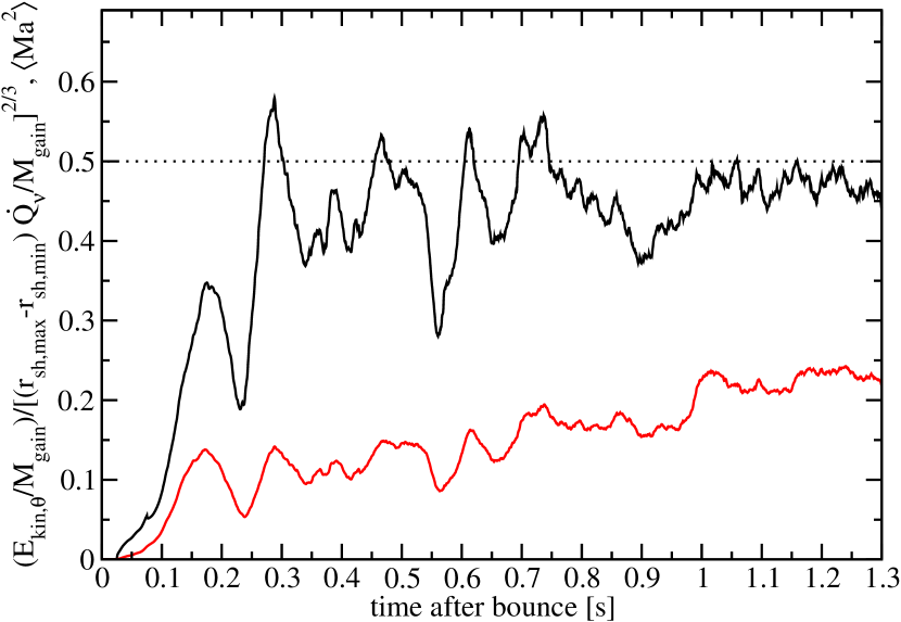
The simulation data for model p0 suggests

$$\frac{E_{\mathrm{kin},\theta}}{M_{\mathrm{gain}}}\approx 0.5\times\left[\frac{(r_{\mathrm{sh,min}}-r_{\mathrm{gain}})\dot{Q}_{\nu}}{M_{\mathrm{gain}}}\right]^{2/3},$$ (25)

as a good approximation for the time-averaged specific kinetic energy in the gain region (Fig. 10) once the SASI and/or convection reach their saturation level, although there are considerable short-term excursions away from this value.

As an alternative to our argument based on the assumption of a self-adjustment to marginal stability to convection, one can derive the scaling law (25) based on the picture of a Carnot engine operating in the supernova core with some crucial modifications of the original idea of Herant et al. (1994). When popularised by Herant et al. (1994) in the 1990s, the heat engine in the supernova core was initially conceived of as powering the explosion itself through a continuous build-up of kinetic energy in the gain region. While this build-up is not observed in modern multi-D simulations like ours, this does not render the thermodynamic analogy with a heat engine invalid; instead a more careful analysis shows why and how the original idea of Herant et al. (1994) and their conclusions about the explosion mechanism must be corrected.

In the heat engine picture, the overturn motions are viewed as an approximate Carnot cycle involving the (roughly) adiabatic transport of cold material from the shock to the gain radius, where it is heated, then expands as it is transported out to the shock and cools by mixing with cold material as the convective/SASI plume dissolves. The mechanical power $\dot{e}_{\mathrm{kin}}$ per unit mass pumped into the instabilities is then given in terms of the heating rate per unit mass $\dot{Q}_{\nu}/M_{\mathrm{gain}}$ as

$$\dot{e}_{\mathrm{kin}}=\frac{T_{\mathrm{gain}}-T_{\mathrm{sh}}}{T_{\mathrm{gain}}}\frac{\dot{Q}_{\nu}}{M_{\mathrm{gain}}},$$ (26)

where the temperatures at the shock, $T_{\mathrm{sh}}$, and at the gain radius, $T_{\mathrm{gain}}$, determine the Carnot efficiency. Since we roughly have $T\propto r^{-1}$ in the gain region, we have

$$\dot{e}_{\mathrm{kin}}=\frac{r_{\mathrm{sh}}-r_{\mathrm{gain}}}{r_{\mathrm{sh}}}\frac{\dot{Q}_{\nu}}{M_{\mathrm{gain}}}.$$ (27)

Herant et al. (1994) proposed this continuous generation of kinetic energy in the heat engine as a means to power the explosion, and this is where their model breaks down: It overlooks the possibility that the Carnot engine reaches a (quasi-)stationary state where the input of mechanical energy is balanced by turbulent dissipation. Dissipation happens at a rate $\varepsilon$ of

$$\varepsilon\sim\frac{\delta v^{3}}{r_{\mathrm{sh}}},$$ (28)

where $\delta v$ and $r_{\mathrm{sh}}$ enter as the typical velocity scale and length scale of the turbulent flow (see § 31 in Landau & Lifshitz 1959). The continuous loss of kinetic energy by downward advection to the cooling region will lead to a term of the same form (kinetic energy density $v^{2}/2$ divided by the advection time-scale $\tau_{\mathrm{adv}}\mathord{\sim}r_{\mathrm{sh}}/v$), and can be thought of as modifying the proportionality constant in the dissipation law.

The condition $\dot{e}_{\mathrm{kin}}\mathord{\sim}\varepsilon$ then immediately leads to equation (24). Instead of the continuous build-up of kinetic energy assumed by Herant et al. (1994), we therefore end up with a saturation of the kinetic energy instead of a runaway. The Carnot engine therefore cannot power continuous shock expansion, but it will nevertheless have an effect on the threshold for runaway shock heating because it creates Reynolds stresses that alter the post-shock stratification and the shock position as we shall see in Section 5.5.

Sometimes we will use a simplified scaling law based on the assumption that $r_{\mathrm{sh,min}}-r_{\mathrm{gain}}\propto r_{\mathrm{sh}}$,

$$\frac{E_{\mathrm{kin},\theta}}{M_{\mathrm{gain}}}\propto\left(\frac{r_{\mathrm{sh}}\dot{Q}_{\nu}}{M_{\mathrm{gain}}}\right)^{2/3}.$$ (29)

This simpler form corresponds to the scaling law obtained by Thompson (2000) (equation 29 in his paper) using a slightly different derivation, which neglected turbulent dissipation and the finite efficiency of the heat engine and instead assumed that all the heating is converted into mechanical energy over one overturn time-scale.

5.4.2 Amplitude of Shock Oscillations

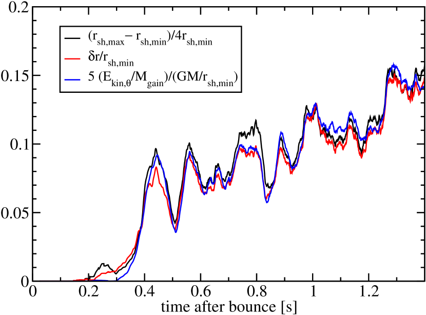
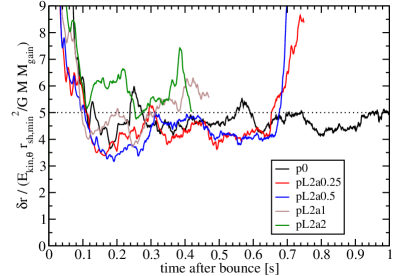
The lateral kinetic energy, which can be taken as a convenient measure for the overall strength of lateral and radial turbulent motions due because of rough equipartition between both components of the turbulent kinetic energy in 2D (Murphy, Dolence & Burrows, 2013), in turn determines the amplitude of shock oscillations. We find a very tight relation between the lateral kinetic energy per unit mass $E_{\mathrm{kin},\theta}/M_{\mathrm{gain}}$, the gravitational potential at the shock radius $GM/r_{\mathrm{sh,min}}$, and the typical deviation $\delta r$ of the shock radius from its spherical average $r_{\mathrm{sh}}=a_{0}$:

$$\delta r=\sqrt{\int\left(r_{\mathrm{sh}}(\theta,\varphi)-a_{0}\right)^{2}\,\mathrm{d}\Omega}.$$ (30)

$\delta r$ can be expressed in terms of the Legendre coefficients $a_{\ell}$ as

$$\delta r=\sqrt{\int\left(r_{\mathrm{sh}}(\theta,\varphi)-a_{0}\right)^{2}\,\mathrm{d}\Omega}=\sqrt{\frac{a_{1}^{2}}{3}+\frac{a_{2}^{2}}{5}+\frac{a_{3}^{2}}{7}+\ldots}.$$ (31)

Fig. 11 shows that for the baseline model

$$\delta r\approx\frac{5E_{\mathrm{kin,\theta}}r_{\mathrm{sh,min}}^{2}}{GMM_{\mathrm{gain}}}$$ (32)

and

$$r_{\mathrm{sh,max}}-r_{\mathrm{sh,min}}\approx 4\delta r\approx\frac{20E_{\mathrm{kin,\theta}}r_{\mathrm{sh,min}}^{2}}{GMM_{\mathrm{gain}}}$$ (33)

hold to good approximation. Note that we have $r_{\mathrm{sh,max}}-r_{\mathrm{sh,min}}\approx 4\delta r$ because the average deviation of the shock radius from its angular average is roughly $(r_{\mathrm{sh,max}}-r_{\mathrm{sh}})/2$, and in turn we have $r_{\mathrm{sh,max}}-r_{\mathrm{sh}}\approx(r_{\mathrm{sh,max}}-r_{\mathrm{sh,min}})/2$.

One can construct a crude physical picture to motivate this scaling relation. If a large bubble produced by SASI or convection is to push out the shock by $\delta r$ in one hemisphere, it must exert work against the pressure of the shocked material flowing around it (which is roughly given by the post-shock pressure $P_{\mathrm{sh}}$). Expansion will cease once the entire kinetic energy of the bubble has been consumed by $P\,\mathrm{d}V$ work. If half of the kinetic energy in lateral motions in the gain region is contained in the hemispheric bubble, then we find

$$2\pi r_{\mathrm{sh}}^{2}P_{\mathrm{sh}}\delta r=\frac{1}{2}E_{\mathrm{kin,\theta}}.$$ (34)

$P_{\mathrm{sh}}$ can be related to the pre-shock ram pressure $\rho_{\mathrm{pre}}v_{\mathrm{pre}}^{2}$ using the jump conditions for a stationary shock,

$$P_{\mathrm{sh}}=\frac{\beta-1}{\beta}\rho_{\mathrm{pre}}v_{\mathrm{pre}}^{2},$$ (35)

where the pre-shock velocity $v_{\mathrm{pre}}$ is a large fraction of the free-fall velocity ($v_{\mathrm{pre}}\approx\sqrt{2GM/r_{\mathrm{sh}}}$), $\rho_{\mathrm{pre}}=\dot{M}/(4\pi r^{2}v_{\mathrm{pre}})$ is the pre-shock density, and $\beta$ is the ratio of the post-and pre-shock densities. Expressing $P_{\mathrm{sh}}$ in term of the post-shock density $\rho_{\mathrm{sh}}$, we find

$$P_{\mathrm{sh}}\approx\frac{\beta-1}{\beta^{2}}\frac{\rho_{\mathrm{sh}}GM}{r_{\mathrm{sh}}},$$ (36)

and hence obtain

$$\frac{2\pi r_{\mathrm{sh}}^{2}\delta r(\beta-1)\rho_{\mathrm{sh}}GM}{\beta^{2}r_{\mathrm{sh}}}=\frac{1}{2}E_{\mathrm{kin,\theta}}.$$ (37)

Since $\rho_{\mathrm{sh}}\propto M_{\mathrm{gain}}/(4/3\pi r_{\mathrm{sh}}^{3})$, this implies

$$\frac{3\delta r(\beta-1)M_{\mathrm{gain}}GM}{2\beta r_{\mathrm{sh}}^{2}}\propto\frac{1}{2}E_{\mathrm{kin,\theta}},$$ (38)

and hence a scaling law for $\delta r$ of the form of equation (32),

$$\delta r\propto\frac{E_{\mathrm{kin,\theta}}r_{\mathrm{sh,min}}^{2}}{GMM_{\mathrm{gain}}}.$$ (39)

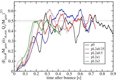
Alternatively, the scaling law may be written in terms of the typical (squared) turbulent Mach number of lateral motions in the post-shock region, $\langle\mathrm{Ma}^{2}\rangle$, which we define as

$$\langle\mathrm{Ma}^{2}\rangle=\frac{\langle v_{\theta}^{2}\rangle}{c_{\mathrm{s,post}}^{2}}=\frac{2E_{\mathrm{kin,\theta}}/M_{\mathrm{gain}}}{c_{\mathrm{s,post}}^{2}}.$$ (40)

Here, the post-shock sound speed $c_{\mathrm{s,post}}$ is given in terms of by $P_{\mathrm{sh}}$, $\rho_{\mathrm{sh}}$, and the adiabatic index $\Gamma$ as:

$$c_{\mathrm{s,post}}^{2}=\frac{\Gamma P_{\mathrm{sh}}}{\rho_{\mathrm{sh}}}=\Gamma\frac{\beta-1}{\beta^{2}}v_{\mathrm{pre}}^{2}=\Gamma\frac{\beta-1}{\beta^{2}}\frac{2GM}{r_{\mathrm{sh,min}}}\approx\frac{GM}{3r_{\mathrm{sh,min}}},$$ (41)

if we use $\beta\approx 7$ and $\Gamma=4/3$. One can easily verify that equation (32) can thus be written as

$$\frac{\delta r}{r_{\mathrm{sh,min}}}\approx\frac{5}{6}\langle\mathrm{Ma}^{2}\rangle.$$ (42)

Figure 12: Comparison of the average shock radius (top left), the criticality parameter $\tau_{\mathrm{adv}}/\tau_{\mathrm{heat}}$ (top right), the mass in the gain region $M_{\mathrm{gain}}$ (bottom left), and the kinetic energy contained in lateral fluid motions $E_{\mathrm{kin},\theta}$ (bottom right) for the baseline model p0 and selected models from the pL2aX series.

5.5 The Impact of Non-Radial Instabilities on the Heating Conditions

Presently, we still lack a quantitative theory for describing how multi-dimensional instabilities facilitate runaway shock expansion. While both parameterized and first-principle simulations have established that multi-dimensional effects are beneficial for the heating conditions in the supernova core, different concepts may be and have been used to interpret these findings, many of which date back already to the first generation of multi-dimensional supernova models in the 1990s (see, e.g., Herant et al., 1994; Burrows, Hayes & Fryxell, 1995). On the one hand, it can be argued that turbulent stresses (Murphy, Dolence & Burrows, 2013; Müller, Janka & Heger, 2012; Couch & Ott, 2014), heating by secondary shocks during the non-linear SASI phase (Müller, Janka & Heger, 2012) and convective energy transport alter the (spherically averaged) post-shock flow, enhance the mass in the gain region, and thereby bring the supernova core closer to the critical condition $\tau_{\mathrm{adv}}/\tau_{\mathrm{heat}}$ for runaway heating. On the other hand, one might view the possibility of asymmetric shock expansion driven by large neutrino-heated bubbles (Thompson, 2000; Burrows, Dolence & Murphy, 2012; Dolence et al., 2013; Couch, 2013a; Fernández et al., 2014) as the crucial factor for facilitating explosions in multi-D.

These different viewpoints are by no means incongruent with each other, and it is difficult to decide which picture is most appropriate as a causal explanation on the basis of simulation data. Nevertheless, it is desirable to have a rough diagnostic quantity for the global influence of multi-dimensional effects in the supernova core. We argue that the typical Mach number of non-radial velocities in the gain region is an appropriate measure for assessing how efficiently multi-dimensional instabilities assist neutrino heating in the development of a runaway instability.

The pivotal role of the “turbulent” Mach number $\mathrm{Ma}$ in the post-shock region can be illustrated by considering two very crude models for an explosive runaway aided by multi-dimensional instabilities. If we incorporate the effect of turbulent stresses as an additional isotropic pressure contribution $P_{\mathrm{turb}}\approx\langle\delta v^{2}\rangle\rho\approx 4/3\langle\mathrm{Ma}^{2}\rangle P$ throughout the gain region into the derivation of the relation for the critical luminosity (19), we obtain

$$L_{\nu}E_{\nu}^{2}\propto(\dot{M}M)^{3/5}r_{\mathrm{gain}}^{-2/5}\left(1+\frac{4\langle\mathrm{Ma}^{2}\rangle}{3}\right)^{-3/5}$$ (43)

because the higher post-shock pressure results in a larger shock radius compared to equation (13),

$$r_{\mathrm{sh}}\propto\frac{(L_{\nu}E_{\nu}^{2})^{4/9}r_{\mathrm{gain}}^{16/9}\left(1+\frac{4\langle\mathrm{Ma}^{2}\rangle}{3}\right)^{2/3}}{\dot{M}^{2/3}M^{1/3}}$$ (44)

and a longer advection time-scale (see Appendix B). A large turbulent Mach number therefore leads to a reduction of the critical luminosity in this simple model. Note that $\langle\mathrm{Ma}^{2}\rangle$ is a function of the heating conditions here and hence depends $L_{\nu}$, $E_{\nu}$, $r_{\mathrm{gain}}$, $\dot{M}$, $M$, and also $r_{\mathrm{sh}}$ itself. Surprisingly, this simple model can roughly predict the observed reduction of the critical luminosity by $\mathord{\sim}20\%$ in multi-D compared to 1D, as we show in Appendix B.

On the other hand, if we view the emergence of a large, expanding high-entropy bubble as the critical element in multi-dimensional explosions (Thompson, 2000; Burrows, Dolence & Murphy, 2012; Dolence et al., 2013; Couch, 2013a; Fernández et al., 2014), we can formulate an alternative runaway condition. If the buoyant acceleration of such a bubble is to overcome the drag of the infalling material flowing around it, the density contrast $\delta\rho/\rho$ to the surrounding matter must exceed a critical limit (Fernández et al., 2014),

$$\left(\frac{\delta\rho}{\rho}\right)\sim\frac{C_{D}v_{\mathrm{post}}^{2}}{2gl}.$$ (45)

Here, $C_{D}$ is the drag coefficient, $v_{\mathrm{post}}$ is the post-shock velocity, $g=GM/r_{\mathrm{sh}}^{2}$ is the gravitational acceleration at the shock, and $l$ is the ratio of the volume of the bubble to its cross-section. Since $\delta\rho/\rho\sim\langle\mathrm{Ma}^{2}\rangle$ (see § 10 in Landau & Lifshitz 1959), this is again a critical condition involving the turbulent Mach number:

$$\langle\mathrm{Ma}^{2}\rangle\sim\frac{C_{D}v_{\mathrm{post}}^{2}}{2gl}.$$ (46)

If we assume that the volume-to-surface ratio $l$ is given by the shock radius (e.g. $l\sim r_{\mathrm{sh}}/2$) when runaway expansion sets in, this condition can be cast into an even simpler form,

$$\langle\mathrm{Ma}^{2}\rangle\sim\frac{C_{D}v_{\mathrm{post}}^{2}r_{\mathrm{sh}}}{2GM}\sim C_{D}\beta^{-2},$$ (47)

where $\beta$ is the ratio of the post- and pre-shock densities. As the turbulent velocities are related to the heating conditions, this also implies a critical condition for the neutrino luminosity and mean energy. Using equations (13,16, 29,41) to express the lateral kinetic energy $E_{\mathrm{kin,\theta}}$ in terms of the neutrino heating $\dot{Q}_{\nu}$, and $\dot{Q}_{\nu}=\eta_{\mathrm{heat}}L_{\nu}$ (with $\eta_{\mathrm{heat}}$ taken from equation 16) in terms of $L_{\nu}$, $E_{\nu}$, and $r_{\mathrm{gain}}$, we obtain

$$\langle\mathrm{Ma}^{2}\rangle=\frac{2E_{\mathrm{kin,\theta}}/M_{\mathrm{gain}}}{c_{\mathrm{s,post}}^{2}}\propto\frac{\left(r_{\mathrm{sh}}\dot{Q}_{\nu}/M_{\mathrm{gain}}\right)^{2/3}}{GM/r_{\mathrm{sh}}}\propto\left(\frac{r_{\mathrm{sh}}L_{\nu}E_{\nu}^{2}}{r_{\mathrm{gain}}^{2}}\right)^{2/3}\left(\frac{r_{\mathrm{sh}}}{GM}\right)$$ (48)

for the turbulent Mach number in terms of $L_{\nu}$, $E_{\nu}$, $r_{\mathrm{gain}}$, $\dot{M}$ and $M$. Equation (13) allows us to eliminate the shock radius in favour of $L_{\nu}$, $E_{\nu}$, $r_{\mathrm{gain}}$, $M$, and $\dot{M}$:

$$\langle\mathrm{Ma}^{2}\rangle\propto\frac{(L_{\nu}E_{\nu}^{2})^{2/3}r_{\mathrm{sh}}^{5/3}}{r_{\mathrm{gain}}^{4/3}M}\propto\frac{(L_{\nu}E_{\nu}^{2})^{38/27}r_{\mathrm{gain}}^{44/27}}{\dot{M}^{10/9}M^{14/9}}$$ (49)

The critical condition $\langle\mathrm{Ma}^{2}\rangle\sim C_{D}\beta^{-2}$ will thus be reached for a critical luminosity given by

$$L_{\nu}E_{\nu}^{2}\propto C_{D}^{27/38}\beta^{-27/19}\dot{M}^{15/19}M^{21/19}r_{\mathrm{gain}}^{-22/19}\propto C_{D}^{0.71}\beta^{-1.42}\dot{M}^{0.79}M^{1.11}r_{\mathrm{gain}}^{-1.16}.$$ (50)

Hence, the critical condition for runaway bubble expansion implies that we end up with a relation for the critical luminosity with a relatively similar dependence on $\dot{M}$ as in equation (19), and a somewhat steeper dependence on $M$ and $r_{\mathrm{gain}}$. Given the limited range of variation of $M$ and $r_{\mathrm{gain}}$ and the approximations inherent in the derivation, it seems unlikely that the shape of the critical curve alone (as inferred from simulations) can distinguish between the two pictures of the explosive runaway at shock revival.

The practical use of equation (47) for a quantitative estimate of a “critical Mach number” is limited, however. The geometry of the bubble is a major uncertainty; arguably any value of $l$ in the range $l=r_{\mathrm{sh}}/3\ldots r_{\mathrm{sh}}$ is defensible. Likewise, the drag coefficient $C_{D}$ should be considered as highly uncertain: Simply applying the subsonic drag coefficient $C_{D}\sim 0.5$ of a sphere at intermediate Reynolds numbers may not be adequate, since the bubble has to expand against a supersonic flow from which it is separated by a detached bow shock and a subsonic region of colder, shocked material, which has to be taken into account when computing an effective drag force. Nevertheless, one should still expect the turbulent Mach number in the post-shock region to be a critical factor in the balance between the buoyancy and drag forces even though these complications modify the picture quantitatively.

While admittedly based on two rather crude models for the effect of multi-D instabilities, equations (43) and (50) are very suggestive: In both cases, the reduction of the critical luminosity compared to the 1D case is given by a simple scaling factor (roughly reflecting the findings of Murphy & Burrows 2008, Hanke et al. 2012 and Couch 2013b, a). The average squared Mach number $\langle\mathrm{Ma}^{2}\rangle$ of aspherical motions in the gain layer either enters directly as a critical parameter in equation (47), or regulates the reduction of the critical luminosity by multi-D effects in equation (43). In Section 5.4, we also found that it is the crucial parameter that regulates the shock deformation. There is thus ample motivation for considering $\langle\mathrm{Ma}^{2}\rangle$ as an important measure for the role of multi-D effects in shock revival. Other factors, like the effective drag coefficient for high-entropy bubbles (which depends both on their form and on numerical viscosity) and their surface-to-volume ratio may be of similar relevance for the runaway threshold in multi-D, both are less readily quantifiable.

In order to define a useful volume-integrated measure for the violence of non-radial instabilities, we compare the RMS average of the lateral velocity $v_{\theta}$ to the post-shock sound speed, which is approximately (see equation (41) for a derivation):

$$c_{\mathrm{s,post}}^{2}\approx\frac{GM}{3r_{\mathrm{sh,min}}}.$$ (51)

As in Section 5.4, we define the average squared Mach number $\langle\mathrm{Ma}^{2}\rangle$ in the gain region using this value for $c_{\mathrm{s,post}}^{2}$ as an average over the entire gain region:

$$\langle\mathrm{Ma}^{2}\rangle=\frac{2E_{\mathrm{kin,\theta}}}{M_{\mathrm{gain}}c_{\mathrm{s,post}}^{2}}=\frac{6r_{\mathrm{sh,min}}E_{\mathrm{kin,\theta}}}{GMM_{\mathrm{gain}}}.$$ (52)

$\langle\mathrm{Ma}^{2}\rangle$ is shown in Fig. 10 for the baseline model. There is a steady increase as the heating conditions slowly improve with time.

Figure 13: Modification of the critical luminosity due to seed aspheriticites for the pL2aX series. The approach of the baseline model p0 (solid black curve) to a fiducial critical curve (dashed) in the $(M\dot{M},L_{\nu}E_{\nu}^{2})$ plane is shown as in Fig. 8, i.e. the critical curve is anchored at the final location $(M\dot{M},L_{\nu}E_{\nu}^{2})$ of model p0. The onset of the explosions (defined as the time when $\tau_{\mathrm{adv}}/\tau_{\mathrm{heat}}$ reaches unity) for models pL2a0.25 to pL2a2 (colored lines) is marked by a red circle on each trajectory. Note that the red circles for pL2a0.25 and pL2a0.5 lie on top of each other. As indicated for model pL2a2, the threshold for the explosion is reduced considerably by $\Delta L_{\nu}E_{\nu}^{2}$ for the perturbed models.

Figure 14: Lateral velocity dispersion $\sqrt{\langle v_{\theta}^{2}\rangle}$ (equation 53) for model pL2a2 at a post-bounce time of $385\ \mathrm{ms}$ (top panel) and for model pLa0.25 at a time of $700\ \mathrm{ms}$. The minimum and maximum shock radii are indicated by dotted lines in both panels. The red dashed curve in the top panel is given by the functional expression $9\times 10^{8}\times(r/100\mathrm{km})^{-1}$ and illustrates that $\sqrt{\langle v_{\theta}^{2}\rangle}$ roughly grows like $r^{-1}$ during the infall of shells with similar initial $\sqrt{\langle v_{\theta}^{2}\rangle}$ as predicted by linear perturbation theory. Deviations from this behavior are mainly due to the fact that $\sqrt{\langle v_{\theta}^{2}\rangle}$ is not exactly constant for the initial perturbation pattern, and non-linear effects also play a role.

Figure 15: Snapshots of the entropy $s$ in units of $k_{b}/\mathrm{nucleon}$ (top half of panels) and the lateral velocity $v_{\theta}$ in units of $10^{8}\,\mathrm{cm}\,\mathrm{s}^{-1}$ (bottom half of panels) for model p0 (left column) and model pL2a1 (right column) at post-bounce times of $363\ \mathrm{ms}$, $383\ \mathrm{ms}$, and $403\ \mathrm{ms}$ (top row to bottom row). At this stage, mass shells initially located at a radius of $\mathord{\sim}3000\ \mathrm{km}$ reach the shock. Note that we apply a cut-off for lateral velocities exceeding the minimum and maximum value of the color scale. Arrows indicate the direction of the lateral flow in the post-shock and pre-shock region (if applicable).

6 The Effect of Seed Asphericities on the Explosion Conditions

6.1 Comparison of Heating Conditions for an Exemplary Perturbation Pattern

How do seed asphericities in the progenitor affect the quasi-stationary evolution of the heating conditions and the hydrodynamic instabilities described in Section 5 in such a manner as to shift the onset of the explosion by several hundreds of milliseconds in some cases? A systematic comparison of the heating conditions for model series pL2aX sheds some light on this question. The quadrupolar perturbation pattern is best suited for a such a comparison because the effects of the seed asphericities are already noticeable for moderate seed amplitudes.

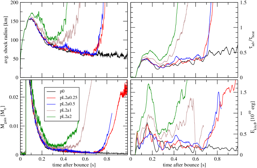
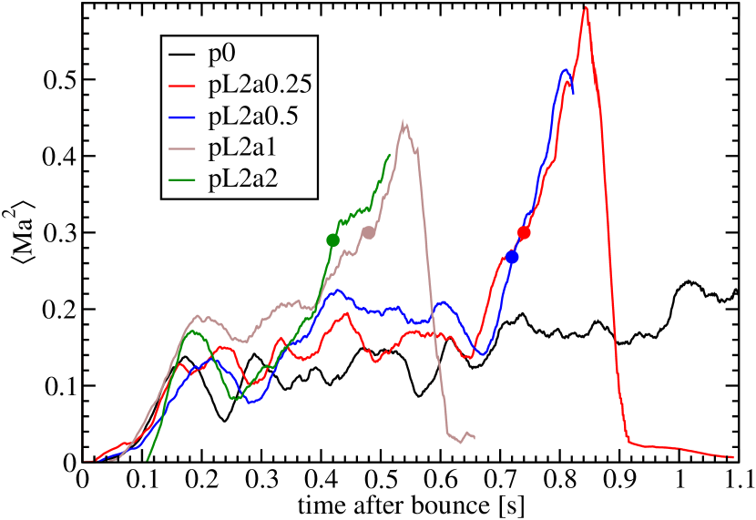
Fig. 12 shows the average shock radius, the criticality parameter $\tau_{\mathrm{adv}}/\tau_{\mathrm{heat}}$, the mass in the gain region, and the kinetic energy contained in lateral fluid motions for selected perturbation amplitudes as well as for the baseline model p0. It is evident that all these diagnostics show a definite hierarchy, reflecting a systematic improvement of the heating conditions and an increasing violence of aspherical motions in the gain region with increasing perturbation amplitude. It is noteworthy that models with different perturbation amplitudes tend to diverge already well before the onset of the explosion.

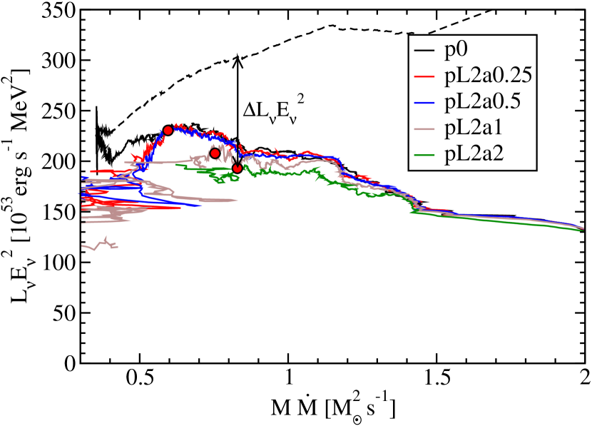
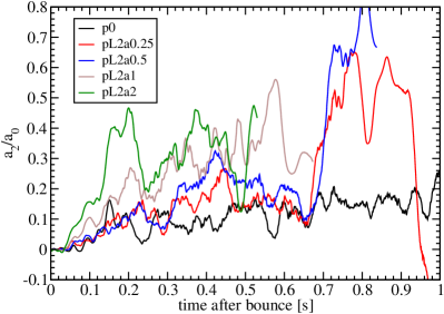
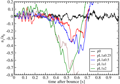
The increase of the pre-explosion value of the criticality parameter already indicates that the critical luminosity required for the initiation of an explosion is reduced dramatically in the more strongly perturbed models. Since the critical curve is essentially defined by $\tau_{\mathrm{adv}}/\tau_{\mathrm{heat}}=1$ (cf. Section 5.3), and $\tau_{\mathrm{adv}}/\tau_{\mathrm{heat}}\propto(L_{\nu}E_{\nu}^{2})^{5/3}$, an increase of $\tau_{\mathrm{adv}}/\tau_{\mathrm{heat}}$ for a given neutrino luminosity must be mirrored by a proportional decrease in the critical luminosity. Models pL2a1 and pL2a2 reach $\tau_{\mathrm{adv}}/\tau_{\mathrm{heat}}=1$ at a time when $\tau_{\mathrm{adv}}/\tau_{\mathrm{heat}}\approx 0.3\ldots 0.4$ in the baseline model, i.e. the baseline model should have reached about $40\%\ldots 60\%$ of the critical luminosity at that junction. Based on the pre-explosion value of $\tau_{\mathrm{adv}}/\tau_{\mathrm{heat}}$ in models pL2a1 and pL2a2, one would therefore estimate a decrease of the critical luminosity of the order of a few tens of percent. This rough estimate can be further corroborated by plotting the evolution of the models in the $(M\dot{M},L_{\nu}E_{\nu}^{2})$ plane (Fig. 13): The perturbed models clearly do not hit the fiducial critical curve constructed for the baseline model p0; instead they break off their approach to the unmodified critical curve around the onset of the explosion and then fall below the $(M\dot{M},L_{\nu}E_{\nu}^{2})$ trajectory of the baseline model. The reduction of the critical luminosity can thus be estimated, it appears to be lower by $15\%$ (pL2a0.25, pL2a0.5) to $40\%$ pL2a2 compared to the baseline model. Naturally, the exact value of the reduction of the critical luminosity is difficult to determine, as it hinges on the precise scaling relation between the time-scale ratio and the neutrino luminosities and mean energies.

A closer inspection of Fig. 13 also reveals a subtle higher-order effect: The trajectories of the more strongly perturbed models (pL2a1 and pL2a2) diverge from the baseline model at a very early stage and consistently show lower values of $L_{\nu}E_{\nu}^{2}$ prior to the onset of the explosion. This implies that for the strongly perturbed post-shock flow in these models, the globally asymmetric post-shock accretion flow onto the proto-neutron star leads to a net decrease of the neutrino emission. While this slight reduction of the total neutrino luminosity is a potentially important phenomenon, we refrain from analyzing it in detail in this paper since be believe that a more rigorous transport scheme is required to verify the existence of this effect.

It is obvious that progenitor asphericities somehow lead to more violent turbulent motions in the gain region that help to push the shock out, increase the mass in the gain region, and thus boost the efficiency of neutrino heating. However, our model allows us to describe this mechanism more precisely.

It appears that the direct injection of kinetic energy into the gain region by the advection of lateral velocity perturbations to and through the shock plays at most a subdominant role. This is suggested by a comparison of the density-weighted lateral velocity dispersion $\sqrt{\langle v_{\theta}^{2}\rangle}$,

$$\sqrt{\langle v_{\theta}^{2}\rangle}=\sqrt{\frac{\int\rho v_{\theta}^{2}\,\mathrm{d}\Omega}{\int\rho\,\mathrm{d}\Omega}},$$ (53)

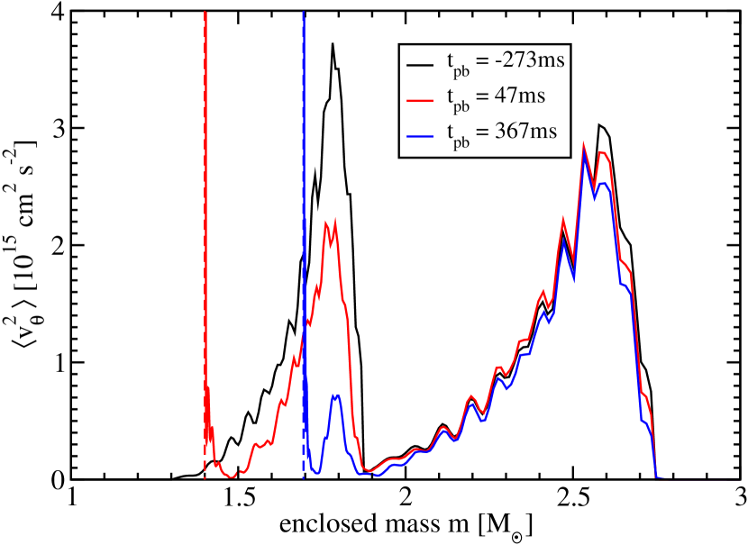
in the pre- and post-shock region. If we assumed that the lateral velocity perturbations were simply advected through a stationary spherical shock, then $\sqrt{\langle v_{\theta}^{2}\rangle}$ should be continuous across the shock front and should scale roughly as $\sqrt{\langle v_{\theta}^{2}\rangle}\sim r^{-1}$ according to linear perturbation theory (Lai & Goldreich, 2000; Buras et al., 2006a; Takahashi & Yamada, 2014), which essentially reflects the conservation of local angular momentum. However, Fig. 14 shows that the post-shock values of $\sqrt{\langle v_{\theta}^{2}\rangle}$ are significantly higher than the pre-shock values, even for strongly perturbed models like pL2a2. This implies that the mere quasi-spherical advection of kinetic energy in lateral motions cannot directly account for the increased activity of convection and/or the SASI, especially in the exploding models with lower perturbation amplitudes.

The pre-collapse asphericities must therefore affect the growth and saturation of non-radial hydrodynamic instabilities in a more subtle way. A closer look at the flow geometry of a strongly perturbed model provides further clues: Fig. 15 compares several snapshots of the entropy and lateral velocity for the baseline model p0 and model pL2a1 shortly before the onset of the explosion in the latter. Model p0 exhibits the typical flow features of an $\ell=1$ SASI sloshing mode in the non-linear regime: Expanding bubbles form and collapse alternately in both hemispheres, coherent vorticity waves (clearly seen in the lateral velocity) propagate inward to maintain the SASI cycle, and downflows develop from fast lateral the flows immediately behind the shock, separating from the shock at the triple points. The flow is distinctly quasi-periodic.

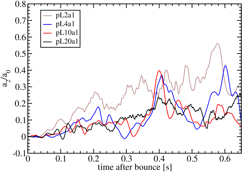
The perturbed model pL2a1 differs from this pattern in some important respects: The post-shock velocity field settles into a relatively stable configuration with two lateral flows colliding near the equator immediately behind the shock, where they form a single persistent downflow. Sloshing motions on top of the stable prolate deformation of the shock are not immediately evident, although a detailed look at the Legendre coefficients of the shock surface still shows some quasi-periodic $\ell=1$ oscillations. The structure of the post-shock flow clearly mirrors the velocity perturbations in the pre-shock region, where we likewise find lateral flows colliding near the equator (and actually forming a double shock). However, the lateral velocities in the pre-shock region are considerably amplified as they fall through the shock at an oblique angle. The permanent prolate deformation of the shock is maintained because the pre-shock flow is strongly anisotropic. Aside from the high lateral velocities in the pre-shock region of the order of $5\times 10^{8}\ \mathrm{cm}\ \mathrm{s}^{-1}$, we find strong deviations from spherical symmetry in the density and the equivalent isotropic mass accretion rate $4\pi\rho v_{r}r^{2}$ as shown in Fig. 16. With these pronounced asphericities in the pre-shock region, the Rankine-Hugoniot jump conditions inevitably result in strong and permanent shock deformation.

Figure 16: Logarithm $\log_{\mathrm{10}}\rho$ of the density (top) and equivalent isotropic mass accretion rate $4\pi\rho v_{r}r^{2}$ in units of $M_{\odot}\ \mathrm{s}^{-1}$ (bottom) for model pL2a1 $403\ \mathrm{ms}$ after bounce.

Figure 17: Normalized Legendre coefficients for the quadrupolar deformation of the shock in model p0 and pL2a0.25 to pL2a2 and for the dipolar deformation in model p0 and pL1a0.25 to pL1a2. Running averages over $20\ \mathrm{ms}$ are applied to reduce high-frequency oscillations and show the secular evolution of the shock deformation more clearly.

Figure 18: Saturation properties of non-radial instabilities for the perturbed models pL2a0.25 to pL2a2 compared to the baseline model p0. The left panel shows the ratio of the RMS shock deformation $\delta r$ and the quantity $\left(E_{\mathrm{kin},\theta}r_{\mathrm{sh,min}}^{2}\right)/(GMM_{\mathrm{gain}})$, and illustrates the approximate validity of equation (32) even in the presence of strong seed perturbations prior to the onset of the explosion. Similarly, the right panel shows the ratio $(E_{\mathrm{kin},\theta}/M_{\mathrm{gain}})/(r_{\mathrm{sh,min}}\dot{Q}_{\nu}/M_{\mathrm{gain}})^{2/3}$ to demonstrate that equation (25) for the relation between neutrino heating and the kinetic energy contained in lateral motions likewise remains valid in the pre-explosion phase. For the sake of clarity, all curves are terminated at the onset of the explosion, and we use running averages over $50\ \mathrm{ms}$ for all quantities.

Figure 19: Average squared Mach number of lateral motions in the gain region for the baseline model p0 and models pL2a0.25 to pL2a2. The onset of the explosion, defined as the time when the criticality parameter $\tau_{\mathrm{adv}}/\tau_{\mathrm{heat}}$ reaches unity, is marked by a filled circle on each curve.

Figure 20: Normalized Legendre coefficients for the quadrupolar deformation of the shock in models pL2a1, pL4a1, pL10a1, and pL20a2 during the pre-explosion phase. Running averages over $20\ \mathrm{ms}$ are applied to reduce high-frequency oscillations and show the secular evolution of the shock deformation more clearly. The perturbation pattern pL2a1 clearly leads to a stronger quadrupolar deformation of the shock than patterns with $\ell>2$.

Figure 21: Lateral velocity dispersion $\langle v_{\theta}^{2}\rangle$ as a function of enclosed mass at different times for model pL20a1 with small-scale $\ell=20$ perturbations. The velocity perturbations in the Si/O shell (between $m\approx 1.4M_{\odot}$ and $m\approx 1.9M_{\odot}$) are strongly damped, whereas the outer convective zone is as yet little affected. Note that the curves show only the pre-shock region; the shock position is indicated by a dashed line. Also note that $\langle v_{\theta}^{2}\rangle$ has been smoothed roughly over the radial extent of the individual convective cells.

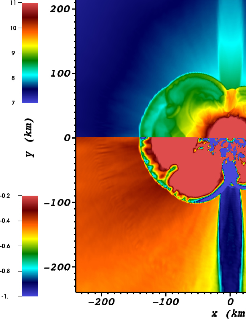
The strong density variations arise despite the solenoidal nature of the initial perturbations for two reasons: First, shocks may form in the course of the non-linear evolution of the perturbations as convective cells collide. More importantly, the spherical isodensity surfaces in the progenitor are distorted during collapse as the infall is accelerated or delayed depending on the initial radial velocity. In order for matter in a convective updraft/downdraft to reach the shock at the same time as matter at rest, it must originate from a different radius with an initial displacement $\delta r$ depending on the radial velocity perturbation $\delta v_{r}$ and the infall time $t$:

$$\delta r\approx\delta v_{r}t.$$ (54)

If the compression factor (i.e. the ratio between the initial density and the pre-shock density) for fluid elements reaching the shock at the same time is identical, this implies Eulerian density perturbations at the shock that depend on the initial density gradient in the progenitor:

$$\frac{\delta\rho}{\rho}\sim\frac{\delta r}{r}\frac{\partial\ln\rho}{\partial\ln r}\sim\frac{\delta v_{r}t}{r}\frac{\partial\ln\rho}{\partial\ln r}\sim\frac{\delta v_{r}}{c_{s}}\frac{\partial\ln\rho}{\partial\ln r}.$$ (55)

The differential infall thus effectively translates radial velocity perturbations into density perturbation of order $\mathcal{O}(\delta v_{r}/c_{s})$ (since the infall time is of the order of the sound-crossing time) instead of $\mathcal{O}(\delta v_{r}/c_{s})^{2}$ during steady-state convection. Conceptually, this amplification mechanism is slightly different from the generation of density perturbations from radial velocity perturbations as investigated by Lai & Goldreich (2000) and Takahashi & Yamada (2014) for the case of supersonic infall. In both cases, density perturbations are essentially generated by the deformation of isodensity contours during the infall, but the available time-scale is $t\approx r/c_{s}$ in our case as opposed to $t\approx r/v_{r}$ ($v_{r}$ being the initial radial velocity in the unperturbed accretion flow) in the setup of Lai & Goldreich (2000) and Takahashi & Yamada (2014).

We surmise that these two factors – the “forced oblate asphericity” of the shock due to the anisotropic mass flux through the shock and the generation of high lateral velocities by an oblique shock – are primarily responsible for increasing the kinetic energy contained in non-spherical instabilities in the presence of strong perturbations. All the exploding models in the pL2aX series are characterized by a considerably stronger quadrupolar deformation than in the baseline model prior to the onset of the explosion as can be seen from Fig. 17, which shows the normalized Legendre coefficient $a_{2}/a_{0}$ for several of these models. This finding is not confined to the perturbation pattern pL2: The onset of the explosion in perturbed models is always associated with a stronger $\ell=2$ (and/or $\ell=1$) deformation of the shock than in the baseline model.

Figure 22: RMS density fluctuations (equation 62 ) ahead of the shock at $r=250\ \mathrm{km}$ for model pDL2a2 (black) and model pL2a0.5 (blue) with quadrupolar density and velocity perturbations, respectively. Overall, the density fluctuations in these two models are of similar magnitude, although there are phase differences). Consequently, these two models explode at a similar time shortly after $700\ \mathrm{ms}$ after bounce.

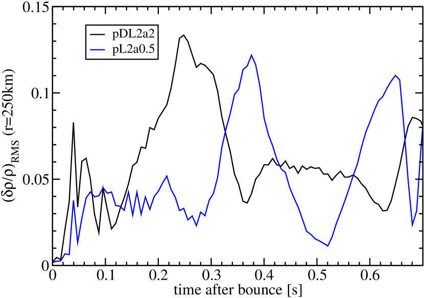
6.2 Saturation of Instabilities in the Presence of Strong Seed Asphericities

It is noteworthy that the saturation of the non-radial instabilities in the perturbed models is still regulated by the amount of heating as in the baseline model. Fig. 18 shows that equations (25) and (32) describe the relation between the volume-integrated neutrino heating rate $\dot{Q}_{\nu}$, the lateral kinetic energy in the gain region $E_{\mathrm{kin},\theta}$, and the average shock deformation $\delta r$ reasonably well even in the presence of strong pre-shock asphericities. This is not inconsistent with our assumption that the forced asphericity of the shock is responsible for the increased violence of SASI and/or convection, but rather suggests that the saturation level is determined by a feedback process: The forced deformation of the shock increases the kinetic energy in non-radial motions in the gain region, this in turn leads to a larger shock radius and a higher mass in the region, which in turn boosts the activity of hydrodynamics instabilities (as reflected by the factor $(r_{\mathrm{sh,min}}-r_{\mathrm{gain}})$ in equation (25)). In the pre-explosion phase, the positive feedback ceases at some point when the further excursions of the shock no longer help to boost the violence of convective and SASI motions effectively enough to permanently sustain a large shock radius. The saturation level will depend both on the overall parameters of the accretion flow (accretion rate, proto-neutron star radius, neutrino luminosity) and on the additional forcing due to seed perturbations in the progenitor. The amplification of the shock deformation by this feedback effect may become less important for very strong forcing, however. Model pL2a2 may be a possible example for the transition to this regime of very strong forcing; here the shock deformation $\delta r$ is somewhat higher than suggested by equation (32).

The fact that neutrino heating and the saturation level of aspherical instabilities are still related by equations (25) and (32) implies that it is impossible to distinguish whether the improvement of the time-scale ratio $\tau_{\mathrm{adv}}/\tau_{\mathrm{heat}}$ due to the expansion of the shock or the easier formation of large buoyant bubbles is more crucial for facilitating the onset of the explosion in the presence of strong progenitor asphericities. Equations (25) and (32) show that the heating conditions, the shock deformation (and hence the typical size of high-entropy bubbles) are inextricably linked to each other and to the typical density perturbation $\delta\rho/\rho$ in the post-shock flow through the turbulent Mach number through equation (42) (since $\delta\rho/\rho\sim\langle\mathrm{Ma}^{2}\rangle$). In particular, there is a remarkable correlation between the criticality parameter $\tau_{\mathrm{adv}}/\tau_{\mathrm{heat}}$ and $\langle\mathrm{Ma}^{2}\rangle$ at the onset of the explosion: At the time of the explosion ($\tau_{\mathrm{adv}}/\tau_{\mathrm{heat}}=1$), all models also appear to reach a “critical Mach number” $\langle\mathrm{Ma}^{2}\rangle\approx 0.3$ in the gain layer (Fig. 19 and Appendix B).

Incidentally, Fig. 18 also shows that the initial perturbations do not have a major effect on the approach to non-linear saturation. The seed for the SASI (which is clearly the instability that grows during the first $\mathord{\gtrsim}100\ \mathrm{ms}$) is already provided by the asphericities left from prompt convection. Progenitor asphericities from the silicon and oxygen shell can only start to make themselves felt a few tens of milliseconds after bounce when they reach the shock, and at this stage, the SASI has already reached sizeable amplitudes. Only afterwards do we see a weak trend (superimposed over considerably stochastic variations) towards slightly faster saturation in models with strong initial perturbations. Since the initial perturbations affect the heating conditions and the saturation of post-shock instabilities primarily through the conversion of initial radial velocity perturbations into density perturbations, their effect becomes strongest only when the middle of the initial “convection zone” (where $|v_{r}|$ is highest) reaches the shock.

6.3 Sensitivity to Perturbation Patterns

6.3.1 Spatial Scale of the Seed Asphericities

The mechanism outlined for the models of the pL2aX series works far less efficiently for perturbations dominated by higher angular wavenumbers $\ell>2$, and also somewhat less efficiently for $\ell=1$ than for $\ell=2$ (see Table 4).

The behavior at $\ell>2$ may be related to the stability properties of the standing accretion shock. Naturally, pre-shock asphericities will more efficiently excite modes that are already unstable; they may excite other modes as well, but if the damping time-scale (due to linear damping or non-linear damping by parasitic instabilities) for such stable modes is short, the resulting amplitude will be negligibly small. This reasoning already suggests that only low-$\ell$ modes can be efficiently excited in the SASI-dominated regime. In the convectively dominated regime, modes with higher angular wavenumber may be excited as well, but the most unstable wavenumber also shifts towards lower $\ell$ as the ratio of the shock radius and gain radius $r_{\mathrm{sh}}/r_{\mathrm{gain}}$ increases. We therefore expect that the pre-shock asphericities need to be able to excite $\ell=1$ or $\ell=2$ perturbations in that case as well in order to increase the violence of convective motions up to the point of shock revival. Perturbations with high $\ell$ may initially excite small-scale convection in the gain region effectively, but the small “overlap” with large-scale modes will render further excitation inefficient once increased convective overturn pushes the shock out.

Since all our velocity perturbation patterns with $\ell>2$ eventually develop some $\ell=2$ component during the infall, we still find explosions in many of these cases. As for the pL2aX series, the explosion is preceded by a strong quadrupolar deformation of the shock, but for comparable kinetic energies contained in the velocity field of the initial perturbations, the normalized quadrupole amplitude is considerably lower (Fig. 20). The degree of “overlap” with the $\ell=2$ mode of the shock is probably crucial for triggering the explosion, and since this overlap depends on the detailed evolution of the asphericities during the infall, one cannot expect a simple monotonic dependence on $\ell$. High-$\ell$ perturbations will generally develop less overlap with the $\ell=2$ mode, but on the other hand, an $\ell=2$ component may emerge faster in these cases because the typical evolution time-scale of the convective cells is smaller (see below). Moreover, the forcing changes rapidly in time because of the small radial extent of the individual convective eddies in the models with higher $\ell$.

The non-linear damping of the pre-collapse perturbations in the subsonic infall region is another factor contributing to the less efficient excitation of instabilities in the gain region in the case of high $\ell$. Non-linear effects will start to come into play on the crossing time-scale for convective cells, which is approximately

$$t_{\mathrm{cell}}\approx\frac{r\pi}{\ell\ |v_{\theta,\mathrm{max}}|}.$$ (56)

For a model like pL20a1, we have $t_{\mathrm{cell}}\approx 0.5\ \mathrm{s}$, and consequently, the pre-shock perturbations are damped considerably over the course of the simulation. Since the collapse time until core bounce is already $273\ \mathrm{ms}$ for the $15M_{\odot}$ progenitor, the initial perturbations in the Si/O shell are damped considerably. This is illustrated by Fig. 21, which shows the evolution of the lateral velocity dispersion $\langle v_{\theta}^{2}\rangle$ in the pre-shock region.

Overall, our findings are compatible with the weak trend towards a more efficient excitation of aspherical motions in the post-shock layer seen by Couch & Ott (2014) for initial perturbations with smaller $\ell$. However, they suggest that i) the limited investigation of perturbation of different scales by Couch & Ott (2014) may have missed the most interesting case of $\ell=1$ and $\ell=2$, and that ii) the dependence on $\ell$ for $\ell>2$ may not be monotonic and arise from a combination of various factors.

While the small effect of perturbations with high $\ell$ is thus relatively easy to understand, the case of perturbations with $\ell=1$ presents something of a conundrum. While the $\ell=1$ mode of the SASI is clearly unstable, we do not obtain explosions for dipolar perturbations below $\mathrm{Ma}_{\theta,\mathrm{expl}}=0.19$, whereas models with quadrupolar perturbations explode even for $\mathrm{Ma}_{\theta,\mathrm{expl}}=0.05$. Several credible explanations for this behavior can be adduced:

1. Due to the different aspect ratio of the convective cells and the solenoidal constraint, the radial velocity perturbations are smaller by a factor of $\mathord{\sim}2$ in the pL1aX series than in the pL2aX series for the same lateral velocity dispersion $\langle v_{\theta}^{2}\rangle$ (see Table 2). Consequently, smaller density perturbations are generated during the infall, cf. equation (55).

2. In the pL2aX series, we encounter converging flows near the equator, which can steepen into a double shock (Figs. 15 and 16). The formation of such a double shock results in a significantly increased mass flux onto the shock in a narrow wedge around the equator. Presumably, this helps to stabilize the quadrupolar shock deformation and the post-shock flow geometry with the very persistent, almost radial downflow near the equator.

3. Models with strong dipolar shock deformation develop a very pronounced neutrino emission asymmetry. The neutrino luminosities are considerably lower below the high-entropy bubble, and are enhanced in the hemisphere where the shock radius is smaller. Presumably, the reduction of the neutrino heating in the high-entropy bubble delays the explosive runaway compared to the case of a quadrupolar perturbation pattern. For quadrupolar perturbations, the matter funneled into the cooling region through the equatorial downflow can still be redistributed relatively efficiently to higher latitudes to radiate neutrinos into the polar high-entropy bubbles.

While the hemispheric emission anisotropy may be a generic factor hampering shock revival in models with dipolar perturbations, the more efficient generation of density perturbations in models with quadrupolar perturbations depends very much on the precise convective flow geometry in the progenitor. We therefore believe that it would be premature to state that dipolar asphericities are generically less effective as a means of facilitating shock revival. Only better models for the multi-D flow structure of convection in the progenitor will allow definite conclusions.

6.3.2 Location and Extent of Convective Regions

Our results clearly demonstrate that the location of the convective regions is a crucial factor in determining whether pre-collapse asphericities can aid shock revival or not: Models for which the initial perturbations are restricted to the unstable regions according to mixing-length theory (pPAaX, pPSaX, pPDaX) explode at late times at best.

While only moderate convective Mach numbers are required to bring about an explosion in some of these models (e.g. $\mathrm{Ma}_{\theta,\mathrm{expl}}=0.07$ in model pPSa2, see Table 4), we find two problems that thwart early shock revival: As the inner convective zones are extremely narrow, we expect that convection is dominated by high-$\ell$ modes ($\ell\sim 10$) in these zones, which makes it difficult to excite large-scale shock deformations. On the other hand, the convective shell driven by neon burning is very wide and is probably dominated by low-$\ell$ modes for that reason, but it only reaches the shock at very late times. Between $\mathord{\sim}200\ \mathrm{ms}$ and $\mathord{\sim}700\ \mathrm{ms}$ after bounce, the infalling mass shells are therefore essentially spherical (except for acoustic waves and gravity waves generated at the convective boundaries). Regardless of their amplitude, pre-collapse asphericities therefore cannot trigger explosions much earlier than $\mathord{\sim}700\ \mathrm{ms}$ after bounce if convective activity is restricted to the regions where mixing-length theory predicts instability.

The location and width of the convective regions may, however, be highly sensitive to the zero-age main sequence mass and other stellar parameters as well as to the treatment of convection, semiconvection, convective overshoot, and angular momentum transport in stellar evolution calculations. As for the flow geometry and the typical scale of the convective eddies, we have to defer final answers until multi-D models of supernova progenitors at the onset of collapse become available.

6.3.3 Non-solenoidal vs. Solenoidal Perturbations

The purely transverse velocity perturbation pattern (pCOaX) inspired by the setup of Couch & Ott (2013) proves about as efficient at triggering shock revival as the solenoidal perturbation pattern with $\ell=2$, which implies that the effective reduction of the critical luminosity is also of the order of several tens of percent. Superficially, this strong effect appears to be somewhat at odds with the results of Couch & Ott (2013), which suggest that the critical luminosity is smaller by only $\mathord{\sim}2\%$ in their perturbed models.

However, the huge impact of transverse velocity perturbations in our simulations can easily be accounted for. In all pCOaX models, large density anisotropies develop during the infall simply because the initial perturbations are non-solenoidal as shown by a simple rule-of-thumb estimate: The time derivative of the density is given by the divergence of the momentum density field,

$$\frac{\partial\rho}{\partial t}=-\nabla\cdot(\rho\mathbf{v}+\rho\mathbf{\delta v}),$$ (57)

from which we can split off a component $(\partial\rho/\partial t)_{\mathrm{infall}}$ due to compression, by the spherical background flow,

$$\frac{\partial\rho}{\partial t}=\left(\frac{\partial\rho}{\partial t}\right)_{\mathrm{infall}}-\rho\nabla\cdot\mathbf{\delta v}-\mathbf{\delta v}\cdot\nabla\rho.$$ (58)

Since $\mathbf{\delta v}\cdot\nabla\rho=0$ (i.e. the velocity perturbations are orthogonal to the density gradient), density perturbations will develop during the infall following

$$\frac{1}{\rho}\frac{\mathrm{d}\delta\rho}{\mathrm{d}t}=-\nabla\cdot\mathbf{\delta v}.$$ (59)

With the typical size $L$ of the convective cells, the density contrast grows like

$$\frac{\delta\rho}{\rho}\sim\frac{t\delta v}{L},$$ (60)

or

$$\frac{\delta\rho}{\rho}\sim\frac{t\ell\delta v}{\pi r}.$$ (61)

if $\ell$ is the typical angular wavenumber. Since the sound crossing time-scale is of the order of the infall time for the small $\ell$ considered here, non-linear damping and pressure equilibration can be neglected to zeroth order.

Although density perturbations at the shock arise for completely different reasons, the expected level of density fluctuations is similar to the one given by equation (55) in the case of solenoidal perturbations for similar perturbation amplitudes. Moreover, the density perturbations arising during the infall have a strong $\ell=2$ component that can couple to the $\ell=2$ mode of the shock.

Although these factors imply that purely lateral velocity perturbations are very efficient at facilitating shock revival, Couch & Ott (2013) nonetheless obtained only a minute effect in their 3D simulations for several reasons. Whether or not the forced deformation of the shock due to pre-shock asphericities is genuinely weaker in the 3D case is a moot point, but the perturbation pattern of Couch & Ott (2013) differs from our pCOaX models in that there is an additional modulation in the $\varphi$-direction, and the overlap with the $\ell=2$ mode of the shock is presumably much smaller for this reason. Furthermore, Couch & Ott (2013) treat neutrino heating and cooling by means of a simple leakage scheme, which results in a strong and unfavorable temporal variation of the heating conditions during the early accretion phase: In their unperturbed baseline model, the time-scale ratio $\tau_{\mathrm{adv}}/\tau_{\mathrm{heat}}$ transiently rises to $0.6$ around $130\ \mathrm{ms}$ after bounce and then plummets rather abruptly to only $0.1$ within a hundred milliseconds. This leaves only a short time window for pre-shock perturbations to achieve sufficient shock expansion to push the model above the critical threshold. Obviously, it is difficult to quantify the impact of progenitor asphericities for such highly non-stationary heating conditions, and the reduction of the critical heating parameter $f$ of Couch & Ott (2013) by $2\%$ may not fully reflect the potential of pre-shock perturbations to aid shock revival.

6.3.4 Density Perturbations vs.  Velocity Perturbations

The foregoing discussion has already made it clear that the efficient conversion of velocity perturbations into density perturbations and into an anisotropic mass flux onto the shock is the key to efficient shock revival in the perturbed models. Since pure density perturbations in the initial model only grow moderately during collapse ($\delta\rho/\rho\propto r^{-1/2}$ in the linear regime according to Lai & Goldreich 2000; Takahashi & Yamada 2014), it is evident that relatively strong initial density perturbations are required to produce an appreciable effect. According to equation (55), velocity perturbations translate into density perturbations at the shock of the order of the initial convective Mach number, i.e. $\delta\rho/\rho\propto\mathrm{Ma}_{\mathrm{prog}}$, whereas the initial density perturbations should only be of the order of $(\delta\rho/\rho)_{\mathrm{ini}}\sim\mathrm{Ma}_{\mathrm{prog}}^{2}$ (at least in the interior of the convective zones), and even moderate amplification during the infall will not create as large anisotropies in the mass flux onto the shock as in the case of initial velocity perturbations of the same convective Mach number.

However, if the initial density perturbations are large enough to produce pre-shock density fluctuations of the same magnitude as in models with velocity perturbations, the effect on shock revival is similar. This can be illustrated by comparing the density fluctuations ahead of the shock for the two models pL2a0.5 and pDL2a2, which explode at a similar time. Fig. 22 shows the RMS fluctuations of the density around the spherical average $\bar{\rho}$,

$$\left(\frac{\delta\rho}{\rho}\right)_{\mathrm{rms}}=\frac{1}{\bar{\rho}}\sqrt{\frac{1}{4\pi}\int(\rho-\bar{\rho})^{2}\,\mathrm{d}\Omega},$$ (62)

at a radius of $250\ \mathrm{km}$. Both models show a similar level of pre-shock density fluctuations, especially at the time of shock revival. This can be interpreted as further evidence that the anisotropic pre-shock density field is the primary factor responsible for enhancing the heating conditions in strongly perturbed models.

Since initial density perturbations of the order of $\delta\rho/\rho\gg\mathrm{Ma}_{\mathrm{prog}}^{2}$ appear to be required in order to achieve any appreciable effect, it seems likely that convective density fluctuations in the progenitor play a subdominant role for supernova dynamics compared to convective velocity perturbations. In order to obtain sufficiently large density perturbations, physical mechanisms other than convection probably need to be invoked, such as rotation or unstable g-modes (Murphy, Burrows & Heger, 2004).

A detailed analysis of the infall dynamics reveals a further complication in the setup of initial perturbations. In the models with density perturbations, we observe relatively strong acoustic waves propagating inside of and beyond the perturbed region. These acoustic waves can lead to a considerable modification of the initial angle-dependence of the density perturbations during the infall. Sometimes the sign of the density perturbations is even reversed, e.g. the initial model may show a density enhancement at the poles, while the perturbations arriving at the shock show higher densities in the equatorial region. This is simply a consequence of the fact that we perturb the density only and keep the temperature fixed, which results in pressure fluctuations $\delta P/P\sim 0.5\delta\rho/\rho$ for the moderate entropies in the perturbed regions. However, this does not strongly change the dependence of the typical amplitude of the pre-shock density perturbations on the initial perturbations $\delta\rho/\rho\sim\mathrm{Ma}_{\mathrm{prog}}^{2}$. The acoustic component of the perturbations will only reach the shock faster and with a different phase than the advected density perturbations.

The actual level of acoustic wave activity present in convective zones in the progenitor cannot be easily predicted. Within mixing-length theory, one assumes complete pressure equilibration of convective bubbles with their surroundings, i.e. $\delta P=0$. By contrast, turbulence theory would suggest that pressure and density fluctuations are similar, i.e. $\delta P/P\propto\delta\rho/\rho\propto\mathrm{Ma}_{\mathrm{prog}}^{2}$ (cp. equation (31.4) and § 10 in Landau & Lifshitz 1959 in Landau & Lifshitz 1959). However, this is a minor concern here, since we expect the role of density perturbations in the progenitor for shock revival to be subdominant anyway.

Interestingly, it appears to be important whether densities are enhanced in the equatorial region or in the polar region. In model pDL2a2m, the sign of $\delta\rho/\rho$ is reversed in the initial perturbation pattern, resulting in a higher mass inflow rate at the poles compared to the equator (which is reversed compared to the initial angular dependence of the perturbations, see our earlier remarks on the role of acoustic waves in models with density perturbations). Different from model pDL2a2, this model fails to explode, indicating that the excitation of an oblate deformation of the shock is less conducive to runaway bubble expansion. Incidentally, the fact that an oblate shock deformation does not boost the heating conditions as effectively as a prolate shock deformation also explains the counterintuitive cases where a larger perturbation amplitude prevents shock revival (as for model pPSa4 compared to pPSa2, see Table 4): In model pPSa2, a quadrupolar density perturbation with lower densities near the axis of the spherical polar grid is present around the onset of the explosion due to the interaction of waves generated at the inner boundary of the outermost convection zone, whereas these secondary waves do not give rise to density perturbations that would lead to an oblate shock. In the outermost convective zone itself, the perturbation patterns leads to overdensities near the axis, i.e. to a hurtful, oblate shock deformation. Because the different fate of these two models is entirely due to the different geometry of secondary perturbations arising from non-linear interactions at the convective boundary (e.g. acoustic waves excited as the artificially imposed eddies distort the boundary), a higher initial perturbation amplitude can indeed prove harmful in such special cases.

7 Summary and Conclusions

Using relativistic 2D simulations with multi-group neutrino transport, we have performed an extensive parameter study to investigate whether progenitor asphericities arising during convective burning could play a crucical role in the supernova explosion mechanism. Our investigation is based on a detailed quantitative analysis of the interplay of neutrino heating and aspherical instabilities, which provides a framework for understanding the role of seed perturbations, but is also an important step towards understanding shock revival in multi-D in its own right. Different from the recent works of Couch & Ott (2013, 2014), we systematically vary the amplitude and geometry of the initial perturbations and investigate both velocity and density perturbations. We also discuss some of the physical principles governing the typical velocities, the density contrast, and the flow geometry in the inner shells of supernova progenitors, and attempt to incorporate some of these principles into our models. Our simulations indicate that even moderate velocity perturbations in the progenitor can aid shock revival rather effectively if low-$\ell$ modes dominate the convective flow in the shells outside the iron core. Furthermore, the analysis of our simulations has unearthed some interesting semi-empirical scaling laws that govern the relation between neutrino heating and the activity of aspherical instabilities in our 2D models.

The main results of our study may be summarized as follows:

1. In our quantitative analysis of the interplay of neutrino heating and non-radial instabilities, we find evidence for quasi-stationary saturation of the SASI and/or convection in the gain region in all our models. The neutrino heating, the shock deformation, the typical turbulent velocities and the turbulent Mach number, $\sqrt{\langle\mathrm{Ma}^{2}\rangle}$, in the gain region are all related to each other by simple scaling laws: At saturation, the dispersion of the lateral velocity in the gain region, $\langle v_{\theta}^{2}\rangle$, is related to the neutrino heating per unit mass, $\dot{q}_{\nu}$, and the width of the gain region, $\delta r_{\mathrm{gain}}$, as $\langle v_{\theta}^{2}\rangle\propto(\delta r_{\mathrm{gain}}\dot{q}_{\nu})^{2/3}$. The deformation of the shock is related to $\langle v_{\theta}^{2}\rangle$ and the gravitational acceleration at the shock $g$ through another scaling relation $\delta r\propto\langle v_{\theta}^{2}\rangle/g_{\mathrm{shock}}\propto\langle\mathrm{Ma}^{2}\rangle$.

2. Based both on the analysis of our numerical simulations and on analytic estimates, we argue that the key towards easier shock revival in multi-D lies in achieving high turbulent Mach numbers in the post-shock flow. We also argue that it is very difficult to ascribe the reduced luminosity threshold for an explosive runaway to a single cause such as more efficient neutrino heating, turbulent stresses, or the formation of large high-entropy bubbles, because in the saturation limit these phenomena are all inextricably related to each other and regulated by the violence of aspherical motions in the post-shock region (for which the turbulent Mach number is a useful measure).

3. Despite these ambiguities, we show that one can construct a simple analytic model that takes into account how turbulent pressure in the post-shock region pushes the shock further out and thereby enhances the heating conditions. Our analytic estimate suggests that the critical luminosity is lowered by roughly $25\%$ in multi-D compared to 1D, and that an explosive runaway occurs when the squared turbulent Mach number $\langle\mathrm{Ma}^{2}\rangle$ in gain region reaches a value of roughly $0.46$ (compared to $\mathord{\sim}0.3$ in the numerical models), both of which is in reasonable agreement with simulations (Murphy & Burrows, 2008; Hanke et al., 2012; Couch, 2013a).

4. Concerning initial perturbations due to convection in the progenitor, we argue that velocity perturbations ought to reflect the subsonic nature of the flow in the convective zones outside the iron core, and should approximately obey the anelastic condition $\nabla\cdot(\rho\,\mathbf{\delta v})=0$, at least away from the convective boundaries. The perturbation pattern of Couch & Ott (2013) strongly violates this condition. Density perturbations $\delta\rho/\rho$ should be of the order of the square of the convective Mach number $\mathrm{Ma}_{\mathrm{prog}}$ in the interior of convective regions.

5. Asphericities in the progenitor enhance the heating conditions primarily because they result in a permanent, “forced” deformation of the accretion shock due to directional variations of the mass infall rate. The shock deformation results in a larger average shock radius and helps to channel the kinetic energy of the infalling material into more violent aspherical motions in the post-shock region as the matter hits the shock at an oblique angle. The very efficient conversion of velocity perturbations $\delta v$ into large density perturbations $\delta\rho/\rho\sim\mathrm{Ma}_{\mathrm{prog}}$ ahead of the shock due to differential infall appears to be a key element of this mechanism because it causes the anisotropy in the mass infall rate.

6. For a given typical amplitude of velocity perturbations, quadrupolar and, to a lesser extent, dipolar perturbations are most efficient at triggering an explosion. For quadrupolar velocity perturbations, convective Mach numbers in the progenitor as low as $0.05$ yield an appreciable effect and reduce the critical luminosity required for shock revival by $\gtrsim 10\%$ according to our estimate, with stronger perturbations having a proportionately larger effect. Even in this conservative case with low convective Mach numbers, shock revival already occurs when the critical time-scale ratio $\tau_{\mathrm{adv}}/\tau_{\mathrm{heat}}$ approaches a value of $\approx 0.5$ in the corresponding unperturbed model.

7. On the other hand, one would have to invoke convective Mach numbers that are probably unrealistically high to achieve similar effects with perturbations dominated by higher angular wavenumbers $\ell$ for several reasons: These modes are inefficient at exciting a permanent $\ell=1$ or $\ell=2$ deformation of the shock, and non-linear damping during the infall comes into play much earlier for small-scale perturbations.

8. Only large density perturbations $\delta\rho/\rho\gtrsim 0.1$ have a significant impact on the heating conditions. Such strong perturbations would probably also require inordinately high convective Mach numbers.

These results have implications on several levels. They suggest that convective perturbations in the progenitor can aid shock revival down to much lower Mach numbers than recently demonstrated by Couch & Ott (2013). Relatively small convective velocities below $10^{8}\ \mathrm{cm}\ \mathrm{s}^{-1}$, which are more in line with 3D simulations of oxygen shell burning (but still higher than predicted by Kuhlen, Woosley & Glatzmaier 2003) may already have a significant impact on the heating conditions. With our present limited knowledge of the multi-dimensional structure of supernova progenitors just prior to collapse, it is therefore still conceivable that asphericities arising from convective burning may be one of the key elements for obtaining robust supernova explosions.

There are, however, some caveats. Our present study is limited to 2D, and it remains to be seen whether the forced deformation of the accretion shock can play the same beneficial role for shock revival in 3D as in 2D. In particular, the relatively efficient excitation of quadrupole modes could be ascribed to the presence of an (artificial) symmetry axis. Unfortunately, a direct comparison with the 3D simulations of Couch & Ott (2013, 2014) is hampered by the fact that we cannot mimic their inherently non-axisymmetric setup in any of our 2D simulations. It is reassuring that the trend towards a more efficient excitation of turbulent motions in the post-shock region for small $\ell$ found by Couch & Ott (2014) is compatible with our findings; however, aside from their use of initial velocity perturbations that lead to an unphysically strong contamination by acoustic waves, their study missed the spot in parameter space ($\ell=1,2$) that emerged as most interesting in our simulations. Clearly, a more systematic study of 3D perturbation geometries with a neutrino treatment on par with or better than our FMT scheme would be highly desirable.

Moreover, our results already place relatively tight constraints on the required properties of the convective flow in the shells outside the iron core. If progenitor asphericities are to have an impact on shock revival, convective Mach numbers need to be of the order of at least $\gtrsim 0.05$, and large-scale dipolar or quadrupolar modes should dominate the flow. Furthermore, extended regions in the progenitor need to be convective, which is by no means a trivial requirement given that 1D stellar evolution calculations predict rather narrow convective shells at least in some cases. Clearly, only 3D simulations covering full $4\pi$ in solid angle and multiple burning shells will finally tell us whether this is indeed the case. They may also reveal whether sufficiently large velocity and density perturbations may arise for other reasons, e.g. because of rotation effects or g-mode activity (Murphy, Burrows & Heger, 2004). The case of rotating progenitors may be particularly interesting because rotation could at least help to organize the flow into large-scale modes (depending on the convective Rossby number). At any rate, self-consistent non-stationary multi-D models of supernova progenitors are urgently needed to replace the ordered laminar flow patterns used in this study, which can never fully capture reality.

Further work is also needed on the conceptual level. While we have been able to provide a qualitative description of the interaction of perturbations in the pre-shock region with the shock and with the hydrodynamic instabilities active in the post-shock region, our results prompt a number of questions: Is the susceptibility of the shock to a forced deformation by $\ell=1$ and $\ell=2$ perturbations more intimately linked to the SASI, which is also a low-$\ell$ instability? How does the saturation of convection and/or the SASI depend on the presence of strong progenitor asphericities? As we consider the role of convective perturbations from the pre-collapse phase in the neutrino-driven mechanism, we are even brought back to some of the more basic questions in supernova modeling: What is the precise mechanism by which aspherical instabilities in the supernova core aid shock revival? Is it by generating turbulent stresses that push the shock out (Murphy, Dolence & Burrows, 2013; Müller, Janka & Heger, 2012; Couch & Ott, 2014) or by facilitating the formation of large high-entropy bubbles (Thompson, 2000; Fernández & Thompson, 2009; Dolence et al., 2013), or by more efficient neutrino heating due to longer dwell times in the gain region (Buras et al., 2006a; Murphy & Burrows, 2008; Marek & Janka, 2009)? In this paper, we have touched many and partially answered some of these questions, collecting and sharpening ideas about the interplay of neutrino heating and hydrodynamic instabilities from the literature and combining them with our analysis of a large suite of 2D simulations with and without initial perturbations. At this junction, it is of course impossible to present a complete picture of the complicated feedback mechanisms linking neutrino heating, non-spherical instabilities, and initial perturbations. Nonetheless, we hope that the ideas presented here may prove fruitful for the analysis of supernova simulations in the future and spark further urgently needed work on the hydrodynamics of the supernova engine.

We acknowledge fruitful exchange with M. Viallet, J. Guilet, Th. Foglizzo, A. Heger, W. Hillebrandt, O. Pejcha, and T. Thompson. This work was supported by the Deutsche Forschungsgemeinschaft through the Transregional Collaborative Research Center SFB/TR 7 “Gravitational Wave Astronomy” and the Cluster of Excellence EXC 153 “Origin and Structure of the Universe” (http://www.universe-cluster.de). B.M. acknowledges support by the Alexander von Humboldt Foundation through a Feodor Lynen fellowship and by the Australian Research Council through a Discovery Early Career Researcher Award (grant DE150101145). The computations were performed on the IBM iDataPlex system hydra at the Rechenzentrum of the Max-Planck Society (RZG), with support by the European PRACE infrastructure on the Curie supercomputer of the Grand Équipement National de Calcul Intensif (GENCI) and on SuperMUC at the Leibniz-Rechenzentrum (LRZ) (with additional computer time from the Gauss Centre for Supercomputing e.V. on that platform), as well as on Raijin at the NCI National Facility (project fh6) and swinStar using our ASTAC allocation for Q2/2014, and on the Monash eGrid Cluster.

Appendix A Fast Multigroup Transport Scheme

Currently, the state of the art in multi-D simulations of core-collapse supernovae is defined by multi-group neutrino hydrodynamics simulations relying on various approximations to reduce the complexity of the general relativistic Boltzmann equation (Livne et al., 2004; Swesty & Myra, 2009; Müller, Janka & Dimmelmeier, 2010; Bruenn et al., 2013; Zhang et al., 2013). While there has been a lot of debate about the merits and demerits of the approximations involved (ray-by-ray-approximation vs. multi-angle transport, general relativity vs. the Newtonian approximation, inclusion or non-inclusion of energy-exchanging scattering reactions, etc.), all these schemes pose similar challenges from the computational point of view. Typically, core-collapse supernova simulations covering several hundreds of milliseconds of the post-bounce phase require $\mathord{\sim}10^{7}$ core-h in 3D and $\mathord{\sim}10^{5}$ core-h in 2D on modern supercomputers. Even in 2D, exhaustive parameter studies with several dozen models are hardly feasible within a reasonable time-frame with these state-of-the-art methods in the light of such extraordinary computational demands.

For our present study with $\mathord{\sim}40$ axisymmetric models, we therefore introduce a new multi-group neutrino transport scheme that captures many of the essential features seen in simulations with more sophisticated methods at a fraction of the computational cost. It is designed as a compromise between more elaborate multi-group schemes and more severe approximations like gray transport (Fryer, Rockefeller & Warren, 2006; Scheck et al., 2006) or the light bulb and leakage schemes (Ruffert, Janka & Schaefer, 1996; Rosswog & Liebendörfer, 2003; Murphy & Burrows, 2008; O’Connor & Ott, 2011) used in many recent studies of multi-dimensional instabilities in core-collapse supernovae. While this new scheme is similar to the IDSA approximation of Liebendörfer, Whitehouse & Fischer (2009) in this respect, its derivation from the Boltzmann equations is more in line with traditional approximation schemes for the radiative transfer equations relying on a closure of the moment equations. Different from current implementations of the IDSA approximation, there is also no need to fall back onto a leakage scheme for the heavy flavor neutrinos.

A.1 Solution of the Monochromatic Neutrino Energy Equation

Our fast multi-group (FMT) scheme solves the stationary neutrino transport problem in the so-called ray-by-ray approximation (Buras et al., 2006b) with the help of a closure relation for the flux factor in the monochromatic neutrino energy equation. As further approximations, we neglect velocity-dependent terms in the transport equation and confine ourselves to isoenergetic scattering.

For a more transparent explanation of the FMT scheme, we also work in the Newtonian approximation in this section and disregard neutrino pair reactions for the moment. The generalization of the FMT scheme to the relativistic case is given in Section A.3, and the neutrino physics input (including a derivation of an effective one-particle rate for nucleon bremsstrahlung) is described in Section A.5.

Using all these approximations, the monochromatic neutrino energy equation reduces to the simple form

$$\frac{1}{r^{2}}\frac{\partial Hr^{2}}{\partial r}=\kappa_{a}\left(J_{\mathrm{eq}}-J\right),$$ (63)

or

$$\frac{1}{r^{2}}\frac{\partial Hr^{2}}{\partial r}=\kappa_{a}\left(J_{\mathrm{eq}}-\frac{H}{h}\right),$$ (64)

where $J$ and $H$ are the zeroth and first moment of the neutrino intensity, respectively, $J_{\mathrm{eq}}$ is the zeroth moment of the equilibrium distribution function, and $h=H/J$ is the flux factor. $\kappa_{a}$ is the absorption opacity including phase-space blocking effects.

A.1.1 Flux Factor – Interior Solution

At high and intermediate optical depths, we provide the required closure for equation (64) by solving the Boltzmann equation using a two-stream approximation with a radially outgoing and and radially ingoing ray. For the sake of simplicity, we assume purely isotropic scattering. With $f_{o}$ (outgoing) and $f_{i}$ (ingoing) denoting the value of the distribution function in the direction of these two rays, we end up with the following two equations:

$$\frac{\partial f_{o}}{\partial r} = \kappa_{a}\left(f_{\mathrm{eq}}-f_{o}\right)+\kappa_{s}\left(f_{i}-f_{o}\right),$$ (65)

$$-\frac{\partial f_{i}}{\partial r} = \kappa_{a}\left(f_{\mathrm{eq}}-f_{i}\right)+\kappa_{s}\left(f_{o}-f_{i}\right).$$ (66)

Here, $f_{\mathrm{eq}}$ denotes the equilibrium value of the distribution function, and $\kappa_{s}$ is the scattering opacity. Thanks to the choice of the ray directions, there are no angular advection terms in the equations, which therefore remain “quasi-planar” despite the spherical geometry of the transport problem.

Equations (65,66) can be solved by means of a Riccati transformation. After transforming to new variables $f_{+}=(f_{o}+f_{i})/2$ and $f_{-}=(f_{o}-f_{i})/2$, we obtain

$$\frac{\partial f_{+}}{\partial r} = -\left(\kappa_{a}+\kappa_{s}\right)f_{-},$$ (67)

$$\frac{\partial f_{-}}{\partial r} = \kappa_{a}\left(f_{\mathrm{eq}}-f_{+}\right).$$ (68)

Using the ansatz $f_{-}=\psi+\chi f_{+}$, we obtain a valid solution for $f_{o}$ and $f_{i}$ from three equations for $\psi$, $\chi$ and $f_{+}$

$$\frac{\partial\chi}{\partial r} = -\kappa_{a}+\left(\kappa_{a}+\kappa_{s}\right)\chi^{2},$$ (69)

$$\frac{\partial\psi}{\partial r} = \kappa_{a}f_{\mathrm{eq}}+\left(\kappa_{a}+\kappa_{s}\right)\chi\psi,$$ (70)

$$\frac{\partial f_{+}}{\partial r} = -\left(\kappa_{a}+\kappa_{s}\right)\left(\psi+\chi f_{+}\right).$$ (71)

In order to satisfy the correct boundary conditions for $f_{o}$ and $f_{i}$, namely $f_{i}(R_{\mathrm{max}})=0$ and $f_{i}(0)=f_{o}(0)$, we impose the following boundary conditions on $f_{+}$, $\chi$, and $\psi$:

$$\chi(R_{\mathrm{max}})=1,\quad\psi(R_{\mathrm{max}})=0,\quad f_{+}(0)=-\frac{\psi(0)}{\chi(0)}.$$ (72)

The actual flux factor $h$ that we feed into equation (64) is then computed from $f_{o}$ and $f_{i}$. However, we do not simply compute $h$ using the two-stream approximation as $h=(f_{o}-f_{i})/(f_{o}+f_{i})$. Instead we assume a continuous distribution function of the form

$$f(\mu)=e^{a(\mu-\eta)},$$ (73)

which we fit to the values on the outgoing and ingoing ray ($\mu=\pm 1$) in order to obtain better agreement in the diffusive regime, where $\mathcal{I}(\mu)=J+3\mu H$. The resulting flux factor is

$$h=1+2\frac{2f_{i}/f_{o}}{1-f_{i}/f_{o}}+\frac{2}{\ln f_{i}/f_{o}}.$$ (74)

In the vicinity of the removable singularity at $f_{i}/f_{o}=1$, we use the series expansion

$$h=\frac{1}{6}\left(1-\frac{f_{i}}{f_{o}}\right)+\frac{1}{12}\left(1-\frac{f_{i}}{f_{o}}\right)^{2}\ldots.$$ (75)

Figure 23: Total neutrino luminosities (top panel) and angle-averaged mean energies (bottom panel) for the baseline model p0 as simulated with the FMT scheme (black) and with Vertex-CoCoNuT (red). Solid, dashed, and dotted curves are used for $\nu_{e}$, $\bar{\nu}_{e}$, and $\nu_{\mu/\tau}$, respectively. All quantities are measured at a radius of $400\ \mathrm{km}$.

Figure 24: Top: Time evolution of the maximum, minimum (solid curves), and average (dashed) shock radius, the gain radius (dotted), and the proto-neutron star radius (dash-dotted, defined by a fiducial density of $10^{11}\ \mathrm{g}\ \mathrm{cm}^{-3}$) for the baseline model p0 as simulated with the FMT scheme (black) and with Vertex-CoCoNuT (red). Bottom: The time-scale ratio $\tau_{\mathrm{adv}}/\tau_{\mathrm{heat}}$ in the simulations with the FMT scheme (black) and with Vertex-CoCoNuT (red).

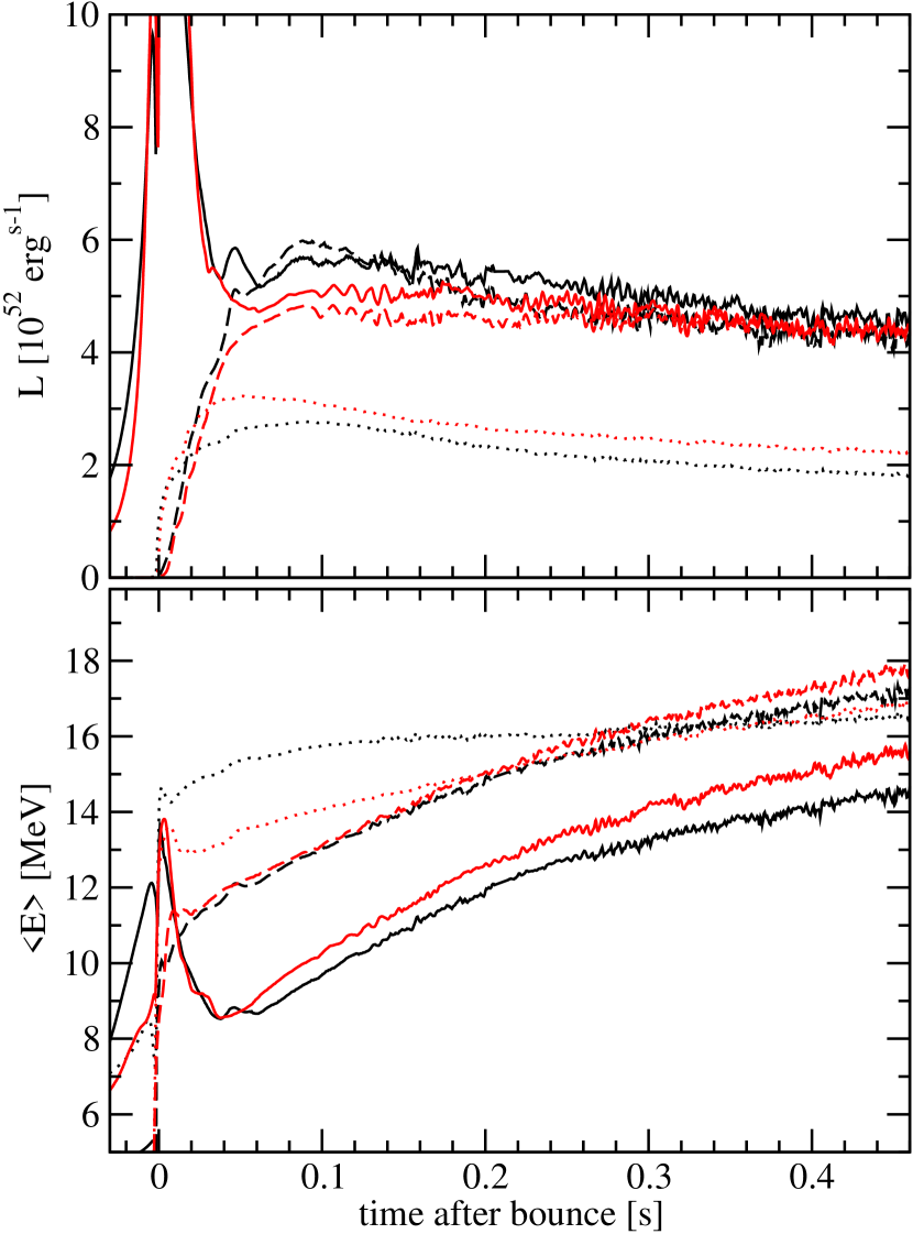
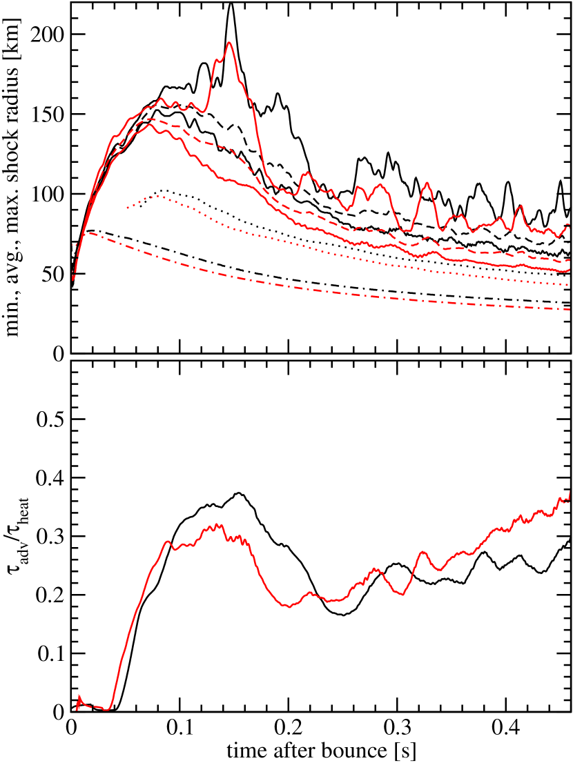
A.1.2 Flux Factor – Transition to Free Streaming

It can easily be seen that the two-stream approximation fails to reproduce the gradual transition of the neutrino radiation field from an isotropic distribution to a forward-peaked distribution towards low optical depths: Instead, equation (74) gives a flux factor of unity as soon as the intensity on the ingoing ray vanishes ($f_{i}=0$), i.e. as soon as emission and scattering reactions cease. In the worst case (e.g. when accretion has died down after the explosion), this would imply that the flux factor abruptly jumps to $h=1$ at the neutrinosphere. On the other hand, the opposite problem can be encountered at moderate optical depths inside the neutrinosphere. Here, the outward propagation of neutrinos in a spherically stratified medium may lead to a faster transition to forward peaking than the two-stream approximation would suggest. This is a consequence of the last term on the left-hand side of the transfer equation in spherical symmetry

$$\frac{\partial\mathcal{I}}{\partial t}+\mu\frac{\partial\mathcal{I}}{\partial r}+\frac{1-\mu^{2}}{r}\frac{\partial\mathcal{I}}{\partial\mu}=C,$$ (76)

where $\mu$ is the angle cosine with respect to the radial direction and $C$ is the collision integral. The last term can essentially be understood as an advection term shifting radiation intensity towards $\mu=1$.

In order to avoid or at least mitigate such unphysical effects inherent in the quasi-planar two-stream approximation, we make the following two modifications: First, we replace the total opacity in equation (67) with a reduced opacity corrected for the advection towards $\mu=1$ in phase space,

$$\kappa_{a}+\kappa_{s}\rightarrow\mathrm{max}\left(\kappa_{a}+\kappa_{s}-\frac{2}{5r},0\right).$$ (77)

Here, the term $2/5r$ is conceived of as an appropriate average over the term $(1-\mu^{2})r^{-1}\partial\mathcal{I}/\partial\mu$ for a nearly isotropic radiation field.

The second modification is more important and consists in matching the “interior solution” for the flux factor to an “exterior solution” once the flux factor from the two-stream approximation exceeds an (adjustable) threshold value $h_{\mathrm{match}}$, which we set to $h_{\mathrm{match}}=0.51$ in this present study. The exterior solution is computed using a closure relation for the Eddington factor $k=K/J$ (where K is the second angular moment of the neutrino intensity). This is achieved by converting the first two moment equations

$$\frac{1}{r^{2}}\frac{\partial r^{2}H}{\partial r}=\kappa_{a}\left(J_{\mathrm{eq}}-\frac{H}{h}\right),$$ (78)

$$\frac{\partial kJ}{\partial r}+\frac{\left(3k-1\right)J}{r}=-\left(\kappa_{a}+\kappa_{s}\right)H,$$ (79)

into an ODE for the flux factor,

$$\frac{\partial h}{\partial r}=\frac{{r^{-1}}h\left[k(h)-1\right]+\kappa_{a}\left[h^{2}-k(h)+k(h)J_{\mathrm{eq}}/J\right]+\kappa_{s}h^{2}}{k(h)-hk^{\prime}(h)},$$ (80)

where the derivative $k^{\prime}$ of the Eddington factor with respect to the flux factor enters in the denominator. Equation (80) is integrated outward from the point where the interior solution reaches $h=h_{\mathrm{match}}$. Obviously, the existence of a singular point of the ODE (80) presents a potential complication (Körner & Janka, 1992). We overcome this problem by choosing $h_{\mathrm{match}}$ and the closure $k(h)$ such that no singular point is encountered in the exterior domain. Specifically, we use

$$k(h)=\frac{1-2h+4h^{2}}{3},$$ (81)

which puts the singular point at $h=1/2$. Our choice of $h_{\mathrm{match}}=0.51$ then ensures that we can integrate equation (80) without encountering any singularity. The closure relation employed here gives a somewhat lower Eddington factor $k(h)$ than other closures proposed in the literature (Minerbo, 1978; Pomraning, 1981; Levermore, 1984; Janka, 1991, 1992; Janka, Dgani & van den Horn, 1992; Cernohorsky & Bludman, 1994) over a wide range of flux factors $h$. This is an unavoidable compromise: Due to the breakdown of the two-stream approximation at low optical depths, it is advisable to move the matching point between the interior and exterior solution to a low flux factor while still avoiding the critical point – even at the expense of a slightly suboptimal choice for the Eddington factor $k(h)$.

A.2 Numerical Solution of the Equations

The numerical solution of equations (64,69,70,71, 80) presents few difficulties. We use the implicit Euler method for the stiff ODEs (64,69,70,71), whereas equation (80) can be integrated using an explicit scheme. Care must be taken to ensure the correct direction of integration: The integration must proceed inward for $\chi$ and $\psi$, and outward for $f_{+}$ in order to respect the boundary conditions. For equation (64), the direction of integration depends on the sign of the flux factor $h$, and implicit finite-differencing automatically ensures that the solutions in patches with $h>0$ and $h<0$ join smoothly at the singular points ($h=0$).

In this study, we solve the FMT equations for 21 exponentially spaced energy group, with the energy at bin centers ranging from $3\ \mathrm{MeV}$ to $197\ \mathrm{MeV}$.

A.3 General Relativistic Case

In the general relativistic case, we assume a stationary metric $g_{\mu\nu}$ with vanishing shift and adopt the isotropic gauge,

$$g_{\mu\nu}=\mathrm{diag}(-\alpha^{2},\phi^{4},r^{2}\phi^{4},r^{2}\sin^{2}\theta\phi^{4}),$$ (82)

where $\alpha$ and $\phi$ are the lapse function and conformal factor. These assumptions are generally valid to good accuracy in supernova cores, and allow us to decouple the solution of the transport equation for different energy groups as in the Newtonian case because the redshifted energy $\hat{\epsilon}=\alpha\epsilon$ ($\epsilon$ being the energy measured by a local observer) is a constant of motion. By grouping neutrinos according to $\hat{\epsilon}$, we can replace equation (64) with a balance equation of the type $\nabla_{\mu}j^{\mu}=s$ for the neutrino number within the $k$-th energy group,

$$\frac{1}{\sqrt{-g}}\frac{\partial}{\partial r}\left(\sqrt{-g}\phi^{-2}\epsilon_{k}^{-1}H_{k}\Delta\epsilon_{k}\right)=\kappa_{a}\epsilon_{k}^{-1}\left(J_{\mathrm{eq,k}}-\frac{H_{k}}{h}\right).$$ (83)

In this equation, $\epsilon_{k}=\alpha^{-1}\hat{\epsilon}_{k}$ and $\Delta\epsilon_{k}=\alpha^{-1}\Delta\hat{\epsilon}_{k}$ are now functions of radius. The factor $\alpha^{-1}$ accounts for the conversion from monochromatic energy densities and fluxes into number densities and fluxes, and the the factor $\phi^{-2}$ on the left-hand side converts the flux density from a local, orthonormal observer frame to the non-orthonormal coordinate frame (whose basis vectors are given by the coordinate derivatives $\partial/\partial x^{i}$).

Equations (65,66) for the two-stream solution of the Boltzmann equation need to be generalized as well. The relativistic Boltzmann equation reads (Lindquist, 1966; Ehlers, 1971; Stewart, 1971),

$$\frac{\mathrm{d}f}{\mathrm{d}\lambda}=\frac{\partial f}{\partial x^{\mu}}\frac{\mathrm{d}x^{\mu}}{\mathrm{d}\lambda}+\frac{\partial f}{\partial p_{\mu}}\frac{\mathrm{d}p_{\mu}}{\mathrm{d}\lambda}=u^{\mu}v_{\mu}C_{\mathrm{local}},$$ (84)

where $u^{\mu}$ is the neutrino four-velocity and $v^{\mu}$ is the four-velocity of the observer in whose frame the collision integral $C_{\mathrm{local}}$ is computed. In our case we have $v^{\mu}=(\alpha^{-1},0,0,0)$ (as we neglect velocity-dependent terms), $u_{o}^{\mu}=(\alpha^{-1},\phi^{-2},0,0)$ for the four-velocity of the outgoing ray, and $u_{i}^{\mu}=(\alpha^{-1},-\phi^{-2},0,0)$ for the ingoing ray. $\mathrm{d}p_{\mu}/\mathrm{d}\lambda$ vanishes for the outgoing and ingoing ray if we assume that the metric is nearly stationary and neglect non-radial derivatives of the metric function in keeping with the ray-by-ray-approximation. Hence, the equations for the two-stream approximation take on a very simple form,

$$\frac{1}{\phi^{2}}\frac{\partial f_{o}}{\partial r} = \left[\kappa_{a}\left(f_{\mathrm{eq}}-f_{o}\right)+\kappa_{s}\left(f_{i}-f_{o}\right)\right],$$

$$-\frac{1}{\phi^{2}}\frac{\partial f_{i}}{\partial r} = \left[\kappa_{a}\left(f_{\mathrm{eq}}-f_{i}\right)+\kappa_{s}\left(f_{o}-f_{i}\right)\right].$$

Essentially, the only difference to equations (65,66) is the factor in front of the radial derivative that accounts for the conversion between coordinate distances and physical distances. The system can be solved exactly along the same lines as in Section A.1.1.

In our current implementation, the exterior solution for the flux factor is not modified in the relativistic case. At least during the first second of the post-bounce phase, the matching radius is located at a fairly large radius so that relativistic effects are already small and can be neglected for the computation of the flux factor in practice, in particular in an approximative scheme as ours.

A.4 Computation of Source Terms

Once the solution for the energy-dependent stationary transport problem has been computed, the neutrino source terms can in principle be calculated directly from the stationary radiation field and the absorption opacity. However, we prefer an indirect method for computing the neutrino source terms for the equations of hydrodynamics. In the CFC metric used in CoCoNuT, the frequency-integrated zeroth moment of the collision integral

$$C_{\mathrm{tot}}^{(0)}=\sum_{k}C_{\mathrm{local},k}\Delta\epsilon_{k},$$ (85)

can be obtained from what is essentially the radial derivative of the redshift luminosity $L_{\infty}=(4\pi)^{2}\alpha^{2}\phi^{4}r^{2}H_{\mathrm{tot}}$,

$$\frac{\partial\phi\alpha^{2}\phi^{4}r^{2}H_{\mathrm{tot}}}{\partial r}=\alpha^{2}\phi^{6}r^{2}C_{\mathrm{tot}}^{(0)},$$ (86)

where $H_{\mathrm{tot}}$ is the frequency-integrated first moment of the neutrino intensity for a stationary solution of the transport equation. The neutrino source term for the energy equation is then computed from $C_{\mathrm{tot}}^{(0)}$ as in Müller, Janka & Dimmelmeier (2010). Although we neglect velocity-dependent effects in our solution for the radiation field, we also follow Müller, Janka & Dimmelmeier (2010) in including a Lorenz boost from the fluid frame to the Eulerian frame, which we found to increase the robustness of the scheme.

The source term in the equation for the electron fraction can be obtained in a completely analogous manner. The required weighted sum $\mathcal{C}_{\mathrm{tot}}^{(0)}$ over the collision integral,

$$\mathcal{C}_{\mathrm{tot}}^{(0)}=\sum_{k}\epsilon_{k}^{-1}C_{k}\Delta\epsilon_{k},$$ (87)

is computed as

$$\frac{\partial\alpha\phi^{4}r^{2}\mathcal{H}_{\mathrm{tot}}}{\partial r}=\alpha\phi^{6}r^{2}\mathcal{C}_{\mathrm{tot}}^{(0)},$$ (88)

where $\mathcal{H}_{\mathrm{tot}}=\sum_{k}\epsilon_{k}^{-1}H_{k}\Delta\epsilon_{k}$. The source term for $Y_{e}$ is then again obtained from $\mathcal{C}_{\mathrm{tot}}^{(0)}$ exactly as in Müller, Janka & Dimmelmeier (2010).

In the present study, the momentum source term due to neutrino interactions is neglected because its effect is small, although its computation is straightforward in principle: The momentum source term in the comoving frame is given by

$$Q_{M}=4\pi\sum_{k}(\kappa_{s}+\kappa_{a})H_{k}\Delta\epsilon_{k},$$ (89)

and must be boosted to the Eulerian frame to obtain the source terms in the momentum and energy equation.

It is worth noting that unlike time-dependent neutrino transport methods, a naive ray-by-ray implementation of the FMT scheme that neglects the lateral advection of neutrinos with the fluid does not lead to spurious convective instability at high optical depths. In time-dependent transport schemes, lateral fluid motions effectively lead to an energy and lepton number exchange between different fluid elements if the neutrinos are not advected with the fluid. In the FMT scheme, on the other hand, neutrinos cannot “lag behind” laterally moving fluid elements, and no instability can occur.

A.5 Treatment of Neutrino Reactions

The FMT scheme assumes as very simple form for the collision integral that includes only the absorption, emission, and isoenergetic scattering of single neutrinos. This places certain restrictions on the neutrino reactions that can be accommodated within the scheme. In our present implementation, we include charged-current reactions of electron neutrinos and antineutrinos neutrinos with nucleons and nuclei, isoenergetic neutrino scattering off nucleons and nuclei, and the production of $\nu_{\mu}$ and $\nu_{\tau}$ by nucleon-nucleon bremsstrahlung. The energy transfer between neutrinos and the medium in the scattering of heavy flavor neutrinos is taken into account approximatively. In the following, we provide a brief explanation of our implementation of these rates, addressing in particular the case of the heavy flavor neutrinos, where we construct effective single-particle absorption opacities for the relevant reactions.

A.5.1 Electron Neutrinos and Antineutrinos

For electron neutrinos and antineutrinos, the dominant opacity sources are absorption on nuclei (during collapse) and nucleons, and the corresponding scattering reactions, which are almost isoenergetic, and the restriction to the simple form of the collision integral is not a severe limitation. In the FMT scheme, these reactions are currently included as in Rampp & Janka (2002) (cf. Bruenn, 1985; Mezzacappa & Bruenn, 1993a), i.e. the recoil energy transfer in scattering reactions is neglected, as are correlation effects at high densities (Burrows & Sawyer, 1998, 1999), weak magnetism (Horowitz, 1997), and the effects of nucleon interaction potentials (Martínez-Pinedo et al., 2012; Roberts, Reddy & Shen, 2012) (although this particular effect can easily be included). Different from Rampp & Janka (2002), we assume all scattering reactions to be isotropic, i.e. we truncate the Legendre expansion of the scattering kernels at the zeroth moment. Neutrino-electron scattering is neglected completely, although it plays an important role in the deleptonization of the core during the collapse phase (Mezzacappa & Bruenn, 1993b).

A.5.2 Heavy Flavor Neutrinos

The situation is different for the heavy flavor neutrinos; here, the principal production processes are pair processes, and non-isoenergetic scattering on nucleons also plays an important role in thermalizing $\mu/\tau$ neutrinos during the accretion phase. A special treatment is therefore required to accommodate these processes even with the simple form for the collision integral assumed in the FMT scheme.

As a production process, we include nucleon-nucleon bremsstrahlung in the limit of vanishing nucleon degeneracy. We compute an effective single particle rate in order to reduce the collision term to the simple form $\kappa_{a}(f_{\mathrm{eq}}-f)$. Our starting point is the form of the collision integral derived by Thompson, Burrows & Horvath (2000) under the assumption of an isotropic radiation field for non-degenerate nucleons (cp. their equation 3.47),

$$\left(\frac{\partial f_{\nu}}{\partial t}\right)_{\mathrm{brems}} = \mathcal{A}\int\limits_{0}^{\infty}\mathrm{d}\epsilon_{\bar{\nu}}\Big{\{}K_{1}\left(\frac{\epsilon}{2k_{b}T}\right)e^{-\epsilon/(2k_{b}T)}$$

$$\left[(1-f_{\nu})(1-f_{\bar{\nu}})-f_{\nu}f_{\bar{\nu}}e^{\epsilon/(k_{b}T)}\right]\Big{\}}.$$

Here $f_{\nu}$ and $f_{\bar{\nu}}$ designate the value of the distribution function of neutrinos of energy $\epsilon_{\nu}$ and antineutrinos of energy $\epsilon_{\bar{\nu}}$, respectively, and $\epsilon=\epsilon_{\nu}+\epsilon_{\bar{\nu}}$. $T$ is the matter temperature, and $K_{1}$ is a modified Bessel function. Various weak interaction constants, non-dimensional factors, and the dependence on the thermodynamic quantities are lumped into the pre-factor $\mathcal{A}$, for which we refer the reader to the original paper of Thompson, Burrows & Horvath (2000). We reduce equation (A.5.2) for $\partial f_{\nu}/\partial t$ to the desired form by assuming a thermal Fermi-Dirac distribution with zero chemical potential for the antineutrino participating in the reaction (and vice versa for $\partial f_{\bar{\nu}}/\partial t$). The term in square brackets then becomes

$$(1-f_{\nu})(1-f_{\bar{\nu},\mathrm{eq}})-f_{\nu}f_{\bar{\nu},\mathrm{eq}}e^{\epsilon/(k_{b}T)}$$ (91)

$$=(1-f_{\nu})\frac{e^{\epsilon_{\bar{\nu}}/(k_{b}T)}}{1+e^{\epsilon_{\bar{\nu}}/(k_{b}T)}}-f_{\nu}\frac{1}{1+e^{\epsilon_{\bar{\nu}}/(k_{b}T)}}e^{\epsilon/(k_{b}T)}$$

$$=(1-f_{\nu})\frac{e^{\epsilon_{\bar{\nu}}/(k_{b}T)}}{1+e^{\epsilon_{\bar{\nu}}/(k_{b}T)}}-f_{\nu}e^{\epsilon_{\nu}/(k_{b}T)}\frac{e^{\epsilon_{\bar{\nu}}/(k_{b}T)}}{1+e^{\epsilon_{\bar{\nu}}/(k_{b}T)}}$$

$$=\left[1-\left(1+e^{\epsilon_{\nu}/(k_{b}T)}\right)f_{\nu}\right]\frac{e^{\epsilon_{\bar{\nu}}/(k_{b}T)}}{1+e^{\epsilon_{\bar{\nu}}/(k_{b}T)}}$$

$$=\left(1+e^{\epsilon_{\nu}/(k_{b}T)}\right)\left(\frac{1}{1+e^{\epsilon_{\nu}/(k_{b}T)}}-f_{\nu}\right)\frac{e^{\epsilon_{\bar{\nu}}/(k_{b}T)}}{1+e^{\epsilon_{\bar{\nu}}/(k_{b}T)}}$$

$$=\left(1+e^{\epsilon_{\nu}/(k_{b}T)}\right)\frac{e^{\epsilon_{\bar{\nu}}/(k_{b}T)}}{1+e^{\epsilon_{\bar{\nu}}/(k_{b}T)}}\left(f_{\nu,\mathrm{eq}}-f_{\nu}\right).$$

By pulling the term $\left(f_{\nu,\mathrm{eq}}-f_{\nu}\right)$ out of the integral in equation (A.5.2), the collision term assumes the desired form $\kappa_{a}(f_{\mathrm{eq}}-f)$ with an effective single-particle opacity $\kappa_{a}$ given by

$$\kappa_{a}=\mathcal{A}\int\limits_{0}^{\infty}\mathrm{d}\epsilon_{\bar{\nu}}K_{1}\left(\frac{\epsilon}{2k_{b}T}\right)e^{-\epsilon/(2k_{b}T)}\left(1+e^{\epsilon_{\nu}/(k_{b}T)}\right)\frac{e^{\epsilon_{\bar{\nu}}/(k_{b}T)}}{1+e^{\epsilon_{\bar{\nu}}/(k_{b}T)}}.$$ (92)

For the numerical evaluation of equation (92), it is sufficient to replace $K_{1}$ with a low-order asymptotic expansion, as the singularity $\epsilon=0$ is never encountered when the integral is computed on an energy grid with finite resolution.

In addition to bremsstrahlung as a production process, we include the scattering reactions on nucleons and nuclei as for electron neutrinos and antineutrinos. However, for the heavy flavor neutrinos, we also take the small recoil energy transfer in neutrino-nucleon scattering into account by means of the following approximation: Since a neutrino of energy $\epsilon$ scattering off a nucleon transfers a fraction of its energy of about $(\epsilon-3k_{b}T)/(m_{n}c^{2})$ to the medium (or gains energy for $\epsilon<3k_{b}T$) (Tubbs, 1979; Janka, 1991), we include an effective absorption opacity $\kappa_{a,\mathrm{\nu N}}$ for this process, which is defined as a fraction of the neutrino-nucleon scattering opacity $\kappa_{s,\mathrm{\nu N}}$.

$$\kappa_{a,\mathrm{\nu N}}=\frac{\left|\epsilon_{\nu}-3k_{b}T\right|}{m_{n}c^{2}}\kappa_{s,\mathrm{\nu N}}.$$ (93)

In the outer layers of the proto-neutron star, where high-energy neutrinos originating from deeper inside the core partly thermalize by scattering on nucleons in a relatively cool medium (i.e. $\langle\epsilon\rangle>3k_{b}T$), this definition ensures an energy transfer to the matter of the right order, and hence an attenuation of the $\nu_{\mu}$ and $\nu_{\tau}$ neutrino luminosity of $\mathord{\sim}5\ldots 10\%$ outside the primary production region as observed in simulations with a rigorous treatment of neutrino-nucleon scattering (Müller, Janka & Marek, 2012).

A.6 Comparison with the Vertex-CoCoNuT Code

To illustrate that the FMT scheme provides a good approximation to more sophisticated transport schemes (such as Boltzmann transport or two-moment transport with a variable Eddington factor closure), we briefly compare the neutrino emission as well as the dynamical evolution of model p0 to a 2D model computed with the Vertex-CoCoNuT code (Müller, Janka & Dimmelmeier, 2010) using the “full set” of neutrino opacities from Müller, Janka & Marek (2012): Figure 23 shows the neutrino luminosities and mean energies for all flavours both using both the FMT scheme and the relativistic Vertex transport module; different from Figure 6, the plot covers only the phase up to $460\ \mathrm{ms}$ after bounce for which Vertex-CoCoNuT simulation data is available. The evolution of the maximum, minimum, and average shock radius, the gain radius, the proto-neutron star radius, and the time-scale ratio $\tau_{\mathrm{adv}}/\tau_{\mathrm{heat}}$ is depicted in Figure 24.

Overall, the neutrino luminosities and mean energies obtained with the FMT scheme follow those obtained with Vertex reasonably well. There most conspicuous differences concern the emission of heavy flavour neutrinos, for which we obtain smaller luminosities and higher mean energies – a result which is not unexpected because our treatment of the heavy flavour neutrino interaction rates is simplified considerably. Interestingly (but again unsurprisingly), the FMT scheme yields a somewhat larger spread between electron neutrino and electron antineutrino mean energies.

It is presumably the weaker cooling due to the reduced emission of heavy flavour neutrinos that mostly drives the dynamical differences between the FMT model and the Vertex model. The proto-neutron star contracts more slowly with the FMT scheme, which in turn results in larger gain radius and shock-radius. Furthermore, the slower contraction of the proto-neutron star leads to a somewhat weaker increase of the electron neutrino and antineutrino mean energies with time. Despite the different contraction of the proto-neutron star, the differences in the heating conditions remain relatively similar, however. The time-scale ratio $\tau_{\mathrm{adv}}/\tau_{\mathrm{heat}}$ is slightly better in the FMT run at early times, but eventually the heating conditions become more more optimistic in the Vertex model.

While a detailed verification of the FMT scheme by cross-comparisons with other neutrino transport codes in the vein of Liebendörfer et al. (2005); Liebendörfer, Whitehouse & Fischer (2009); Müller, Janka & Dimmelmeier (2010), and O’Connor (2014) is beyond the scope of this paper, there is evidently quite good agreement with Vertex-CoCoNuT, especially considering that we compare multi-D runs where differences in the neutrino treatment can lead to important feedback effects. We conclude that the FMT scheme provides a reliable alternative to more sophisticated transport schemes at least for the purpose of our current paper.

Appendix B A Toy Model for the Reduction of the Critical Luminosity in Multi-D

In this paper, we make frequent use of simple power-law expressions for the time-scales $\tau_{\mathrm{adv}}$ and $\tau_{\mathrm{heat}}$ and for other quantities relevant to shock revival in supernovae (in particular in Section 5.3). Most of these relations were derived in Janka (2001, 2012), but many of them are also found in other papers scattered across the literature. Janka (2012) also used the power law expressions for $\tau_{\mathrm{adv}}$ and $\tau_{\mathrm{heat}}$ to reformulate the time-scale criterion $\tau_{\mathrm{adv}}/\tau_{\mathrm{heat}}$ as a critical condition for the neutrino luminosity.

In the interest of clarity, we provide a concise summary of the assumptions and simplifications entering the derivation of these power laws and the critical condition in this Appendix. Furthermore, we show how multi-D effects can be incorporated into the resulting model for the heating conditions by treating them as an isotropic turbulent pressure that aids shock expansion, following the ideas put forth by Murphy, Dolence & Burrows (2013) and Müller, Janka & Heger (2012) in their analyses of multi-D simulations.

B.1 Spherically Symmetric Toy Model of the Gain Region

Our basic ingredient consists of a simple stationary 1D model for the gain region (Janka, 2001), which is assumed to be radiation-dominated with $P\propto T^{4}$ and adiabatically stratified with power law profile of the density $\rho$ and the pressure $P$,

$$P\propto r^{-4},\quad\rho\propto r^{-3}.$$ (94)

Hydrodynamic boundary conditions both for $P$ and $\rho$ are required at the shock. The post-shock quantities are given in terms of the pre-shock density $\rho_{\mathrm{pre}}$ and velocity $v_{\mathrm{pre}}^{2}$ and the compression factor $\beta$ at the shock as,

$$\rho_{\mathrm{sh}}=\beta\rho_{\mathrm{pre}},$$ (95)

$$P_{\mathrm{sh}}=\frac{\beta-1}{\beta}\rho_{\mathrm{pre}}v_{\mathrm{pre}}^{2}.$$ (96)

For $v_{\mathrm{pre}}$, we use a large fraction of the free-fall velocity compatible that is roughly compatible with numerical simulations,

$$v_{\mathrm{pre}}\sim\sqrt{\frac{2GM}{r_{\mathrm{sh}}}},$$ (97)

and $\rho_{\mathrm{pre}}$ is then obtained from the accretion rate $\dot{M}$ as $\rho_{\mathrm{pre}}=\dot{M}/(4\pi r^{2}v_{\mathrm{pre}})$.

In order to fix the shock radius, one additional boundary condition is required. We fix the shock radius by requiring equilibrium between neutrino energy heating and cooling at the gain radius $r_{\mathrm{gain}}$. Since the cooling and heating rates per baryon roughly scale with $T^{6}\propto P^{3/2}$ and $L_{\nu}E_{\nu}^{2}/r_{\mathrm{gain}}^{2}$, respectively, the required boundary condition is

$$P_{\mathrm{gain}}^{3/2}\propto\frac{L_{\nu}E_{\nu}^{2}}{r_{\mathrm{gain}}^{2}},$$ (98)

where $L_{\nu}$ and $E_{\nu}$ are the neutrino luminosity and mean energy (cf. equation 14). The flux factor at the gain radius is implicitly assumed to be fixed.

With these boundary conditions and the assumption of power-law profiles for the density and pressure, one obtains equation (13) for the scaling of the shock radius:

$$r_{\mathrm{sh}}\propto\frac{(L_{\nu}E_{\nu}^{2})^{4/9}r_{\mathrm{gain}}^{16/9}}{\dot{M}^{2/3}M^{1/3}}.$$ (99)

Once the shock radius is determined, the mass in the gain region $M_{\mathrm{gain}}$ and the advection time-scale $\tau_{\mathrm{adv}}=M_{\mathrm{gain}}/\dot{M}$ can be calculated by analytic integration, which gives

$$M_{\mathrm{gain}}\propto\dot{M}r_{\mathrm{sh}}^{3/2}\ln(r_{\mathrm{sh}}/r_{\mathrm{gain}}),$$ (100)

$$\tau_{\mathrm{adv}}\propto r_{\mathrm{sh}}^{3/2}\ln(r_{\mathrm{sh}}/r_{\mathrm{gain}}).$$ (101)

In this paper, we drop the logarithmic correction and work with an empirical power-law instead (cp. equation 12),

$$\tau_{\mathrm{adv}}\propto\frac{r_{\mathrm{sh}}^{3/2}}{\sqrt{M}}\approx 5\ \mathrm{ms}\times\left(\frac{r}{100\ \mathrm{km}}\right)^{3/2}\left(\frac{M}{M_{\odot}}\right)^{-1/2}.$$ (102)

Here the normalization is chosen such that we get a reasonable fit with simulation data even though we neglect the logarithmic term in equation (101). By contrast, the estimate for the heating time-scale (equation 17),

$$\tau_{\mathrm{heat}}\propto\frac{|e_{\mathrm{gain}}|r_{\mathrm{gain}}^{2}}{L_{\nu}E_{\nu}^{2}},$$ (103)

is based on a zeroth-order approximation for the volume-integrated neutrino heating. Essentially, we assume that the entire mass of the gain region is located close to the gain radius and neglect neutrino cooling.

B.2 Incorporation of Turbulent Stresses and Their Effect on Shock Revival

As a zeroth-order approximation, we assume that convection and/or the SASI alter the shock position and hence the runaway condition by providing isotropic turbulent stresses $P_{\mathrm{turb}}$ everywhere. These turbulent stresses are ultimately provided by $P\,dV$ work exerted by neutrino-heated matter as it expands (and is then accelerated by buoyancy due to the density contrast with the ambient medium), i.e. in principle the reservoir of thermal energy in the gain region is permanently tapped to maintain the turbulent motions. The turbulent energy is permanently dissipated back into thermal energy. Although $P\,dV$ work (or buoyant driving) and dissipation merely balance each other in the steady state, the total reservoir of (thermal+kinetic) energy stored in the gain region, will be higher than without turbulent motions. Moreover, due to the short thermal equilibration time-scale at the gain radius, the thermodynamic boundary condition at the gain radius remains unchanged; and as turbulent motions are expected to flatten the entropy gradient (albeit not completely), the temperature, and thermal pressure profiles remain essentially unchanged (except for the change in shock radius) compared to the case without turbulent stresses on the level of precision that our simple analysis can aim for.

Under these assumptions, we can therefore just add the turbulent pressure to the (unchanged) thermal pressure to obtain the total effective pressure $P_{\mathrm{tot}}$ that will then be used to determine the shock position. Using a constant turbulent Mach number for the entire gain region and an adiabatic index $\Gamma=4/3$, the effective total pressure becomes

$$P_{\mathrm{tot}}=P+P_{\mathrm{turb}}=P\left(1+\frac{4\langle\mathrm{Ma}^{2}\rangle}{3}\right).$$ (104)

With the turbulent pressure included the outer boundary condition for the thermal pressure at the shock becomes

$$P_{\mathrm{sh}}\left(1+\frac{4\langle\mathrm{Ma}^{2}\rangle}{3}\right)=\frac{\beta-1}{\beta}\rho_{\mathrm{pre}}v_{\mathrm{pre}}^{2}.$$ (105)

On the other hand, the inner boundary condition remains unchanged, because it is a thermodynamic boundary condition reflecting the balance between heating and cooling at $r_{\mathrm{gain}}$.

With this new boundary condition, one can derive equation (44) for the shock radius,

$$r_{\mathrm{sh}}\propto\frac{(L_{\nu}E_{\nu}^{2})^{4/9}r_{\mathrm{gain}}^{16/9}\left(1+\frac{4\langle\mathrm{Ma}^{2}\rangle}{3}\right)^{2/3}}{\dot{M}^{2/3}M^{1/3}},$$ (106)

as well as equation (43) for the critical luminosity in the presence of an isotropic turbulent pressure,

$$L_{\nu}E_{\nu}^{2}\propto(\dot{M}M)^{3/5}r_{\mathrm{gain}}^{-2/5}\left(1+\frac{4\langle\mathrm{Ma}^{2}\rangle}{3}\right)^{-3/5}.$$ (107)

In order to estimate the reduction of the critical luminosity due to turbulent stresses, we must relate the correction term $\left(1+\frac{4\langle\mathrm{Ma}^{2}\rangle}{3}\right)^{-3/5}$ to the time-scale criterion $\tau_{\mathrm{adv}}/\tau_{\mathrm{heat}}$, and plug in its value at the runaway threshold (which will still be given by $\tau_{\mathrm{adv}}/\tau_{\mathrm{heat}}=1$). To this end, we compute the ratio of the turbulent kinetic energy per unit mass in the gain region and the post-shock sound speed using equation (25) and $c_{\mathrm{s,post}}^{2}\approx GM/(3r_{\mathrm{sh}})$ from equation (41) as approximation for the sound speed,

$$\langle\mathrm{Ma}^{2}\rangle \approx \frac{2E_{\mathrm{kin},\theta}}{M_{\mathrm{gain}}}\frac{3r_{\mathrm{sh}}}{GM}\approx\left[\frac{(r_{\mathrm{sh}}-r_{\mathrm{gain}})\dot{Q}_{\nu}}{M_{\mathrm{gain}}}\right]^{2/3}\frac{3r_{\mathrm{sh}}}{GM}$$

$$\approx \left(\frac{r_{\mathrm{sh}}|e_{\mathrm{gain}}|}{3\tau_{\mathrm{heat}}}\right)^{2/3}\frac{3r_{\mathrm{sh}}}{GM}.$$

Note that we have used $r_{\mathrm{sh}}-r_{\mathrm{gain}}\approx r_{\mathrm{sh}}/3$ to simplify further calculations. The neutrino heating rate has been eliminated in favor the heating time-scale $\tau_{\mathrm{heat}}$ and the average total energy per unit mass in the gain region, $|e_{\mathrm{gain}}|$ (equation (17)), in order to express $\langle\mathrm{Ma}^{2}\rangle$ in terms of the critical time-scale ratio. To arrive at the desired expression, we approximate

$$|e_{\mathrm{gain}}|\approx\frac{GM}{3r_{\mathrm{sh}}},$$ (109)

although this is slightly inconsistent with our former assumption $|e_{\mathrm{gain}}|=\mathrm{const.}$, and use equation (102) to obtain our final result,

$$\langle\mathrm{Ma}^{2}\rangle \approx \left(\frac{GM}{9\tau_{\mathrm{heat}}}\right)^{2/3}\times 100\ \mathrm{km}\times\left(\frac{\tau_{\mathrm{adv}}}{5\ \mathrm{ms}}\right)^{2/3}\left(\frac{M}{M_{\odot}}\right)^{1/3}\frac{3}{GM}$$ (110)

$$\approx 0.4649\times\left(\frac{\tau_{\mathrm{adv}}}{\tau_{\mathrm{heat}}}\right)^{2/3}.$$

The squared Mach number at the onset of the explosion is $0.46$ according to this prediction, which is somewhat higher than the value of $\langle\mathrm{Ma}^{2}\rangle\approx 0.3$ found in Section 6.2, but it is still in the right ballpark. Plugging this result into equation (43) or (107) and comparing to the 1D result without the correction term $\left(1+\frac{4\langle\mathrm{Ma}^{2}\rangle}{3}\right)^{-3/5}$ immediately gives the reduction of the critical luminosity. Our simple toy model predicts that it should be around $75\%$ of the critical luminosity in 1D, which is roughly consistent with numerical simulations (Murphy & Burrows, 2008; Nordhaus et al., 2010; Hanke et al., 2012; Couch, 2013b, a).

We note, however, that there is an important loophole in our derivation of the critical luminosity in 2D: As soon as the turbulent stresses can no longer be modeled as isotropic and as soon as the boundary conditions at the shock change due to an anisotropic mass flux onto the shock, the reduction compared to the 1D case is no longer given by the correction factor $\left(1+4\langle\mathrm{Ma}^{2}\rangle/3\right)^{-3/5}$ alone. This precludes any application of this simple model to the case of asphericities in the progenitor. A simplified analytic description of shock expansion due to global anisotropies in the pre-shock region along similar lines would be a highly desirable goal for the future.

References

- Arnett (1994) Arnett D., 1994, ApJ, 427, 932
- Arnett, Meakin & Young (2009) Arnett D., Meakin C., Young P. A., 2009, ApJ, 690, 1715
- Arnett & Meakin (2011) Arnett W. D., Meakin C., 2011, ApJ, 733, 78
- Asida & Arnett (2000) Asida S. M., Arnett D., 2000, ApJ, 545, 435
- Bazan & Arnett (1994) Bazan G., Arnett D., 1994, ApJL, 433, L41
- Bazan & Arnett (1998) Bazan G., Arnett D., 1998, ApJ, 496, 316
- Blondin, Mezzacappa & DeMarino (2003) Blondin J. M., Mezzacappa A., DeMarino C., 2003, ApJ, 584, 971
- Bruenn (1985) Bruenn S. W., 1985, ApJS, 58, 771
- Bruenn (1986) Bruenn S. W., 1986, ApJL, 311, L69
- Bruenn et al. (2013) Bruenn S. W. et al., 2013, ApJL, 767, L6
- Buras et al. (2006a) Buras R., Janka H.-T., Rampp M., Kifonidis K., 2006a, A&A, 457, 281
- Buras et al. (2006b) Buras R., Rampp M., Janka H.-T., Kifonidis K., 2006b, A&A, 447, 1049
- Burrows (2013) Burrows A., 2013, Reviews of Modern Physics, 85, 245
- Burrows, Dolence & Murphy (2012) Burrows A., Dolence J. C., Murphy J. W., 2012, ApJ, 759, 5
- Burrows & Fryxell (1992) Burrows A., Fryxell B. A., 1992, Science, 258, 430
- Burrows & Goshy (1993) Burrows A., Goshy J., 1993, ApJL, 416, L75+
- Burrows & Hayes (1996) Burrows A., Hayes J., 1996, Physical Review Letters, 76, 352
- Burrows, Hayes & Fryxell (1995) Burrows A., Hayes J., Fryxell B. A., 1995, ApJ, 450, 830
- Burrows & Sawyer (1998) Burrows A., Sawyer R. F., 1998, Phys. Rev. C, 58, 554
- Burrows & Sawyer (1999) Burrows A., Sawyer R. F., 1999, Phys. Rev. C, 59, 510
- Carter & Prakash (2002) Carter G. W., Prakash M., 2002, Physics Letters B, 525, 249
- Cernohorsky & Bludman (1994) Cernohorsky J., Bludman S. A., 1994, ApJ, 433, 250
- Chandrasekhar (1961) Chandrasekhar S., 1961, Hydrodynamic and Hydromagnetic Stability. Clarendon, Oxford
- Chatzopoulos, Graziani & Couch (2014) Chatzopoulos E., Graziani C., Couch S. M., 2014, ArXiv e-prints 1405.4873
- Chen, Heger & Almgren (2013) Chen K.-J., Heger A., Almgren A. S., 2013, Astronomy and Computing, 3, 70
- Couch (2013a) Couch S. M., 2013a, ApJ, 775, 35
- Couch (2013b) Couch S. M., 2013b, ApJ, 765, 29
- Couch & Ott (2013) Couch S. M., Ott C. D., 2013, ApJL, 778, L7
- Couch & Ott (2014) Couch S. M., Ott C. D., 2014, ArXiv e-prints 1408.1399
- Dimmelmeier, Font & Müller (2002) Dimmelmeier H., Font J. A., Müller E., 2002, A&A, 388, 917
- Dolence et al. (2013) Dolence J. C., Burrows A., Murphy J. W., Nordhaus J., 2013, ApJ, 765, 110
- Ehlers (1971) Ehlers J., 1971, in General Relativity and Cosmology, Sachs R. K., ed., pp. 1–70
- Fernández (2012) Fernández R., 2012, ApJ, 749, 142
- Fernández et al. (2014) Fernández R., Müller B., Foglizzo T., Janka H.-T., 2014, MNRAS, 440, 2763
- Fernández & Thompson (2009) Fernández R., Thompson C., 2009, ApJ, 703, 1464
- Foglizzo, Scheck & Janka (2006) Foglizzo T., Scheck L., Janka H.-T., 2006, ApJ, 652, 1436
- Fryer, Holz & Hughes (2004) Fryer C. L., Holz D. E., Hughes S. A., 2004, ApJ, 609, 288
- Fryer, Rockefeller & Warren (2006) Fryer C. L., Rockefeller G., Warren M. S., 2006, ApJ, 643, 292
- Goldreich, Lai & Sahrling (1997) Goldreich P., Lai D., Sahrling M., 1997, in Unsolved Problems in Astrophysics, Bahcall J. N., Ostriker J. P., eds., pp. 269–280
- Guilet, Sato & Foglizzo (2010) Guilet J., Sato J., Foglizzo T., 2010, ApJ, 713, 1350
- Hanke et al. (2012) Hanke F., Marek A., Müller B., Janka H.-T., 2012, ApJ, 755, 138
- Hanke et al. (2013) Hanke F., Müller B., Wongwathanarat A., Marek A., Janka H.-T., 2013, ApJ, 770, 66
- Heger, Langer & Woosley (2000) Heger A., Langer N., Woosley S. E., 2000, ApJ, 528, 368
- Herant, Benz & Colgate (1992) Herant M., Benz W., Colgate S., 1992, ApJ, 395, 642
- Herant et al. (1994) Herant M., Benz W., Hix W. R., Fryer C. L., Colgate S. A., 1994, ApJ, 435, 339
- Horowitz (1997) Horowitz C. J., 1997, Phys. Rev. D, 55, 4577
- Hüdepohl et al. (2009) Hüdepohl L., Müller B., Janka H., Marek A., Raffelt G. G., 2009, Phys. Rev. Lett.
- Janka (1991) Janka H.-T., 1991, PhD thesis, Technische Universität München, (1991)
- Janka (1992) Janka H.-T., 1992, A&A, 256, 452
- Janka (2001) Janka H.-T., 2001, A&A, 368, 527
- Janka (2012) Janka H.-T., 2012, Annual Review of Nuclear and Particle Science, 62, 407
- Janka, Dgani & van den Horn (1992) Janka H.-T., Dgani R., van den Horn L. J., 1992, A&A, 265, 345
- Janka et al. (2012) Janka H.-T., Hanke F., Hüdepohl L., Marek A., Müller B., Obergaulinger M., 2012, Progress of Theoretical and Experimental Physics, 2012, 010000
- Janka & Müller (1996) Janka H.-T., Müller E., 1996, A&A, 306, 167
- Kippenhahn & Weigert (1990) Kippenhahn R., Weigert A., 1990, Stellar Structure and Evolution. Springer, Berlin
- Kiziltan et al. (2013) Kiziltan B., Kottas A., De Yoreo M., Thorsett S. E., 2013, ApJ, 778, 66
- Körner & Janka (1992) Körner A., Janka H.-T., 1992, A&A, 266, 613
- Kuhlen, Woosley & Glatzmaier (2003) Kuhlen M., Woosley W. E., Glatzmaier G. A., 2003, in Astronomical Society of the Pacific Conference Series, Vol. 293, 3D Stellar Evolution, Turcotte S., Keller S. C., Cavallo R. M., eds., p. 147
- Lai & Goldreich (2000) Lai D., Goldreich P., 2000, ApJ, 535, 402
- Landau & Lifshitz (1959) Landau L. D., Lifshitz E. M., 1959, Course of theoretical physics, Vol. VI, Fluid mechanics. Pergamon Press, Oxford
- Lattimer & Swesty (1991) Lattimer J. M., Swesty F. D., 1991, Nucl. Phys. A, 535, 331
- Levermore (1984) Levermore C. D., 1984, JQSRT, 31, 149
- Liebendörfer (2005) Liebendörfer M., 2005, ApJ, 633, 1042
- Liebendörfer et al. (2005) Liebendörfer M., Rampp M., Janka H.-T., Mezzacappa A., 2005, ApJ, 620, 840
- Liebendörfer, Whitehouse & Fischer (2009) Liebendörfer M., Whitehouse S. C., Fischer T., 2009, ApJ, 698, 1174
- Lindquist (1966) Lindquist R. W., 1966, Ann. Phys., 37, 487
- Livne et al. (2004) Livne E., Burrows A., Walder R., Lichtenstadt I., Thompson T. A., 2004, ApJ, 609, 277
- Marek & Janka (2009) Marek A., Janka H., 2009, ApJ, 694, 664
- Marek, Janka & Müller (2009) Marek A., Janka H., Müller E., 2009, A&A, 496, 475
- Martínez-Pinedo et al. (2012) Martínez-Pinedo G., Fischer T., Lohs A., Huther L., 2012, Physical Review Letters, 109, 251104
- Meakin & Arnett (2006) Meakin C. A., Arnett D., 2006, ApJL, 637, L53
- Meakin & Arnett (2007a) Meakin C. A., Arnett D., 2007a, ApJ, 665, 690
- Meakin & Arnett (2007b) Meakin C. A., Arnett D., 2007b, ApJ, 667, 448
- Mezzacappa & Bruenn (1993a) Mezzacappa A., Bruenn S. W., 1993a, ApJ, 405, 669
- Mezzacappa & Bruenn (1993b) Mezzacappa A., Bruenn S. W., 1993b, ApJ, 410, 740
- Minerbo (1978) Minerbo G. N., 1978, JQSRT, 20, 541
- Müller, Janka & Dimmelmeier (2010) Müller B., Janka H., Dimmelmeier H., 2010, ApJS, 189, 104
- Müller & Janka (2014) Müller B., Janka H.-T., 2014, ApJ, 788, 82
- Müller, Janka & Heger (2012) Müller B., Janka H.-T., Heger A., 2012, ApJ, 761, 72
- Müller, Janka & Marek (2012) Müller B., Janka H.-T., Marek A., 2012, ApJ, 756, 84
- Müller & Janka (1997) Müller E., Janka H.-T., 1997, A&A, 317, 140
- Murphy & Burrows (2008) Murphy J. W., Burrows A., 2008, ApJ, 688, 1159
- Murphy, Burrows & Heger (2004) Murphy J. W., Burrows A., Heger A., 2004, ApJ, 615, 460
- Murphy, Dolence & Burrows (2013) Murphy J. W., Dolence J. C., Burrows A., 2013, ApJ, 771, 52
- Murphy & Meakin (2011) Murphy J. W., Meakin C., 2011, ApJ, 742, 74
- Nordhaus et al. (2010) Nordhaus J., Burrows A., Almgren A., Bell J., 2010, ApJ, 720, 694
- O’Connor (2014) O’Connor E., 2014, ArXiv e-prints
- O’Connor & Ott (2011) O’Connor E., Ott C. D., 2011, ApJ, 730, 70
- Özel et al. (2012) Özel F., Psaltis D., Narayan R., Santos Villarreal A., 2012, ApJ, 757, 55
- Pejcha & Thompson (2012) Pejcha O., Thompson T. A., 2012, ApJ, 746, 106
- Pomraning (1981) Pomraning G. C., 1981, JQSRT, 26, 385
- Rampp & Janka (2002) Rampp M., Janka H.-T., 2002, A&A, 396, 361
- Reddy et al. (1999) Reddy S., Prakash M., Lattimer J. M., Pons J. A., 1999, Phys. Rev. C, 59, 2888
- Roberts, Reddy & Shen (2012) Roberts L. F., Reddy S., Shen G., 2012, Phys. Rev. C, 86, 065803
- Rosswog & Liebendörfer (2003) Rosswog S., Liebendörfer M., 2003, MNRAS, 342, 673
- Ruffert, Janka & Schaefer (1996) Ruffert M., Janka H.-T., Schaefer G., 1996, A&A, 311, 532
- Scheck et al. (2006) Scheck L., Kifonidis K., Janka H.-T., Müller E., 2006, A&A, 457, 963
- Schwab, Podsiadlowski & Rappaport (2010) Schwab J., Podsiadlowski P., Rappaport S., 2010, ApJ, 719, 722
- Smartt (2009) Smartt S. J., 2009, AR&A, 47, 63
- Stewart (1971) Stewart J. M., ed., 1971, Lecture Notes in Physics, Berlin Springer Verlag, Vol. 10, Non-equilibrium relativistic kinetic theory
- Suwa et al. (2010) Suwa Y., Kotake K., Takiwaki T., Whitehouse S. C., Liebendörfer M., Sato K., 2010, PASJ, 62, L49+
- Suwa et al. (2013) Suwa Y., Takiwaki T., Kotake K., Fischer T., Liebendörfer M., Sato K., 2013, ApJ, 764, 99
- Swesty & Myra (2009) Swesty F. D., Myra E. S., 2009, ApJS, 181, 1
- Takahashi & Yamada (2014) Takahashi K., Yamada S., 2014, ArXiv e-prints 1408.3503
- Takiwaki, Kotake & Suwa (2014) Takiwaki T., Kotake K., Suwa Y., 2014, ApJ, 786, 83
- Tamborra et al. (2014) Tamborra I., Hanke F., Janka H.-T., Müller B., Raffelt G. G., Marek A., 2014, ApJ, 792, 96
- Tanaka et al. (2009) Tanaka M. et al., 2009, ApJ, 692, 1131
- Thompson (2000) Thompson C., 2000, ApJ, 534, 915
- Thompson, Burrows & Horvath (2000) Thompson T. A., Burrows A., Horvath J. E., 2000, Phys. Rev. C, 62, 035802
- Tubbs (1979) Tubbs D. L., 1979, ApJ, 231, 846
- Utrobin & Chugai (2011) Utrobin V. P., Chugai N. N., 2011, A&A, 532, A100
- Valentim, Rangel & Horvath (2011) Valentim R., Rangel E., Horvath J. E., 2011, MNRAS, 414, 1427
- Weiss et al. (2004) Weiss A., Hillebrandt W., Thomas H.-C., Ritter H., 2004, Cox and Giuli’s Principles of Stellar Structure, by A. Weiss, W. Hillebrandt, H-C. Thomas, H. Ritter. Cambridge, UK: Princeton Publishing Associates Ltd, 2004.
- Woosley & Heger (2007) Woosley S. E., Heger A., 2007, Phys. Rep., 442, 269
- Yakunin et al. (2010) Yakunin K. N. et al., 2010, Classical and Quantum Gravity, 27, 194005
- Zhang et al. (2013) Zhang W., Howell L., Almgren A., Burrows A., Dolence J., Bell J., 2013, ApJS, 204, 7