Canonical coordinates in toric degenerations

Introduction

Mirror symmetry suggests to study families of varieties with a certain maximal degeneration behaviour [CdGP91], [Mo93], [De93], [HKTY95]. In the important Calabi-Yau case this means that the monodromy transformation along a general loop around the critical locus is unipotent of maximally possible exponent [Mo93, §2]. The limiting mixed Hodge structure on the cohomology of a nearby smooth fibre is then of Hodge-Tate type [De93].

An important insight in this situation is the existence of a distinguished class of holomorphic coordinates on the base space of the maximal degeneration [Mo93], [De93]. Explicitly, these canonical coordinates are computed as $\exp$ of those period integrals of the holomorphic $n$-form $\Omega$ over $n$-cycles that have a logarithmic pole at the degenerate fibre. For an algebraic family they are often determined as certain solutions of the Picard-Fuchs equation solving the parallel transport with respect to the Gauß-Manin connection. For complete intersections in toric varieties these solutions can be written as hyper-geometric series. In particular, canonical coordinates are typically transcendental functions of the algebraic parameters. The coordinate change from the algebraic parameters to the canonical coordinates is referred to as mirror map. The explicit determination of the mirror map is an indispensable step in equating certain other period integrals with generating series of Gromov-Witten invariants on the mirror side.

The purpose of the present paper is to address the topic of canonical coordinates in the toric degeneration approach to mirror symmetry developed by Mark Gross and the second author [GS06], [GS10], [GS11]. In this program, [GS11, Corollary 1.31] provides a canonical class of degenerations defined over completions of affine toric varieties. Our main result says that the toric monomials of the base space are canonical in the above sense. In other words, the mirror map is trivial. This is another important hint of the appropriateness of the toric degeneration approach. In particular, we expect that the Gromov-Witten invariants of the mirror are rather directly encoded in the wall structure of [GS11]. Another consequence of our result is that the formal smoothings constructed in [GS11] lift to analytic families. In order to prove this, we construct sufficiently many cycles using tropical methods. The computation of the period integrals over these we then carry out explicitly.

Morrison [Mo93] defines canonical coordinates as follows. Let $f:\mathcal{X}\to T$ be a maximal degenerating analytic family of Calabi-Yau varieties. The fibre over $t\in T$ is denoted $X_{t}$ and the central fibre of the degeneration lies over $0\in T$. Let $D\subset T$ be the critical locus of $f$ where the fibres $X_{t}$ are singular. Assuming $T$ smooth and $D$ to have simple normal crossings denote by $T_{1},\ldots,T_{r}$ the monodromies around the irreducible components of $D$. The endomorphism given as any positive linear combination of $\log T_{1},\ldots,\log T_{r}$ defines the weight filtration $0\subset W_{0}\subset W_{2}\subset\ldots$ on $H_{n}(X_{t},\mathbb{Z})$ for any fixed $t\not\in D$. A vanishing $n$-cycle $\alpha\in W_{0}$ is a generator of $W_{0}$. It is unique up to sign. Let $\Omega$ be a non-vanishing section of $\Omega^{n}_{\mathcal{X}/T}(\log(\mathcal{D}))$, a relative holomorphic volume form with logarithmic poles along $\mathcal{D}=\pi^{-1}(D)$. The fibrewise integral of $\Omega$ over the parallel transport of an element in $W_{2k}$ yields a function on $T$ with a logarithmic pole of order at most $k$. Hence the following definition makes sense.

Definition 0.1 (Canonical coordinates).

Given $\beta\in W_{2}$ one defines a meromorphic function $h_{\beta}$ on the base $T$ by

$$h_{\beta}(t)=\exp\left(-2\pi i\frac{\int_{\beta}\Omega}{\int_{\alpha}\Omega}\right),\quad t\in T\setminus D.$$

Note that taking $\exp$ disposes of the ambiguity of the monodromy around $X_{0}$ which adds multiples of $\alpha$ to $\beta$. If $h_{\beta}$ extends as a holomorphic function to $T$ it is called a canonical coordinate.

We consider the canonical degenerations given in [GS11]. The central fibre $X_{0}$ is constructed from a polarized tropical manifold $(B,\mathscr{P},\varphi)$ and then a formal degeneration $\mathfrak{X}\to\operatorname{Spf}\mathbb{C}\llbracket t\rrbracket$ with central fibre $X_{0}$ is obtained by a deterministic algorithm that takes as input a log structure on $X_{0}$. Mumford’s degenerations of abelian varieties [Mum72] are examples of such canonical degenerations. Degenerating a Batyrev-Borisov Calabi-Yau manifold [BB94] into the toric boundary [Gr05] gives another important example of degenerations with the type of special fibre considered here, with a priori non-canonical algebraic deformation parameters. One obtains (formal) canonical families here by reconstructing the family up to base change from the central fibre via [GS11] (with higher-dimensional parameter space). The resulting base coordinate then coincides with Morrison’s canonical coordinates in Definition 0.1 as follows from the results of this paper. The transformation from the algebraic to the transcendental coordinate is the aforementioned mirror map.

The definition of $(B,\mathscr{P},\varphi)$, which we recall in §2.3, can be found in [GS06, §4.2]. Here $B$ is a real $n$-dimensional affine manifold with singular locus $\Delta$ at most in codimension two. The linear part of its holonomy is integral. The affine manifold comes with a decomposition $\mathscr{P}$ into integral polyhedra and a multi-valued piecewise affine function $\varphi:B\to\mathbb{R}$. The toric varieties given by the lattice polytopes of $\mathscr{P}$ are the toric strata of $X_{0}$. The singular locus $\Delta$ is part of the codimension two skeleton of the barycentric subdivision of $\mathscr{P}$. The function $\varphi$ encodes the discrete part of the log structure, namely toric local neighbourhoods of $X_{0}$ in $\mathcal{X}$, each given by a cone that is the upper convex hull over $\varphi$ on a local patch of $B$.

For $k\in\mathbb{N}$, let $X_{k}$ be the canonical smoothing of $X_{0}$ to order $k$ constructed in [GS11]. If $X_{0}$ is projective then the formal degeneration is induced by a formal family $\hat{\mathcal{X}}\to\operatorname{Spec}(\mathbb{C}\llbracket t\rrbracket)$ of schemes. In any case, at least if $X_{0}$ is compact, there exists an analytic family $\mathcal{X}\to T$ whose restriction to order $k$ coincides with $X_{k}$ (Theorem 2.1). We assume $B$ to be oriented. We define tropical $1$-cycles in $B$ and show how each such determines an $n$-cycle in the nearby fibres $X_{t}$ of $X_{0}$ in $\mathcal{X}$, unique up to adding a vanishing $n$-cycle. Under the simplicity assumption §2.4, we prove that the tropically constructed $n$-cycles generate $W_{2}/W_{0}$, the relevant graded piece of the monodromy weight filtration. We then integrate the canonical $n$-form $\Omega$ on $\mathfrak{X}$ over these cycles and compute the exponential of the result to order $k$ around $0\in T$. Thus despite the logarithmic pole of the integral it makes sense to talk about canonical coordinates for the formal family $\mathfrak{X}\to\operatorname{Spf}(\mathbb{C}\llbracket t\rrbracket)$. The precise statement of the Main Theorem below (Theorem 0.4) requires some explanations that we now turn to.

Let $\Lambda$ and $\check{\Lambda}$ denote the local systems (stalks isomorphic to $\mathbb{Z}^{n}$) of flat integral tangent vectors on $B\setminus\Delta$. Let $i_{*}\Lambda$ and $i_{*}\check{\Lambda}$ be their pushforward to $B$ (these are constructible sheaves). As described in [GS06, §2.1], $X_{0}$ itself can be reconstructed from $(B,\mathscr{P},\varphi)$ together with an element $s$ in $H^{1}(B,i_{*}\check{\Lambda}\otimes\mathbb{C}^{\times})$, see §2.5. This one-cocycle is represented by a collection $(s_{\tau_{0}\subset\tau_{1}})$ for $\tau_{0},\tau_{1}\in\mathscr{P}$ and is called gluing data. If furthermore $B$ is simple (see §2.4) then the log structure on $X_{0}^{\dagger}$ is determined by the gluing data, see [GS06, Proposition 4.25, Theorem 5.2]. Hence, in the simple case, one may view $H^{1}(B,i_{*}\check{\Lambda}\otimes\mathbb{C}^{\times})$ as the moduli space of log structures on $X_{0}$.

Definition 0.2.

A tropical 1-cycle $\beta_{\operatorname{trop}}$ in $B$ is a graph with oriented edges embedded in $B\setminus\Delta$ whose edges $e$ are labelled by a non-trivial section $\xi_{e}\in\Gamma(e,\Lambda|_{e})$. It is subject to the following conditions. Its vertices lie outside the codimension one skeleton $\mathscr{P}^{[n-1]}$ of $\mathscr{P}$ and its edges intersect $\mathscr{P}^{[n-1]}$ in the interior of codimension one cells in isolated points. A vertex is univalent if and only if it is contained in $\partial B$. Finally, at each vertex $v$, the following balancing condition holds

(0.1) $$\sum_{v\in e}\varepsilon_{e,v}\xi_{e}=0.$$

Here $\varepsilon_{e,v}\in\{-1,1\}$ is the orientation of $e$ at $v$.

Similar cycles have been known in the theory of completely integrable Hamiltonian systems, see [Sy03, Theorem 7.4]. In the context of the Gross-Siebert program, similar tropical cycles have been used by [CBM13]. The balancing condition is a typical feature in tropical geometry, see [Mi05].

Example 0.3.

(Tropical cycles from the $1$-skeleton) Let $\mathscr{P}^{[1]}$ denote the set of one-dimensional cells in $\mathscr{P}$. For a vertex $v\in\mathscr{P}$ with $\omega\in\mathscr{P}^{[1]}$ an edge containing it, we denote by $d_{v,\omega}$ the primitive integral tangent vector to $\omega$ pointing from $v$ into $\omega$. Then for any weight function $a:\mathscr{P}^{[1]}\to\mathbb{Z}$ and any vertex $v\in\mathscr{P}$ we can check the analogue of the balancing condition (0.1) at $v$:

$$\sum_{\omega\ni v}a(\omega)d_{v,\omega}=0.$$

Assuming this balancing condition holds for every $v$ we can then define a tropical $1$-cycle by taking the graph with edges $\{\omega\in\mathscr{P}^{[1]}\,|\,a(\omega)\neq 0\}$ and the embedding into $B\setminus\Delta$ a small perturbation of the $1$-skeleton to make the resulting cycle disjoint from $\Delta$ and its intersection with $\mathscr{P}^{[n-1]}$ discrete. To define the section $\xi_{e}$ and the orientation for the edge $e$, we choose a vertex $v$ of every edge $\omega$. Now the section $\xi_{e}\in\Gamma(e,\Lambda)$ of the edge $e$ of $\beta_{\operatorname{trop}}$ arising as a perturbation of $\omega\in\mathscr{P}^{[1]}$ is defined by parallel transport of $a(\omega)\cdot d_{v,\omega}$ and we orient $e$ by $d_{v,\omega}$. Note that $d_{v,\omega}$ is invariant under local monodromy around $\Delta$, so local parallel transport is uniquely defined. Choosing the other vertex of $\omega$ instead results in a double sign change, namely in the orientation of $e$ as well as in the section $\xi_{e}$ and so the choice of vertex $v$ is insignificant.

A special case of this example arises if $(B,\mathscr{P},\varphi)$ is the dual intersection complex of a degeneration with normal crossing special fibre. The one-skeleton at each vertex then looks like the fan of projective space. As the primitive generators of the rays in this fan are balanced, any non-trivial constant weight function $w:\mathscr{P}^{[1]}\to\mathbb{Z}$ yields a tropical $1$-cycle by the above procedure. This way, one obtains a generator for $W_{2}/W_{0}$ for the mirror dual Calabi-Yau of a degree $(n+1)$-hypersurface in $\mathbb{P}^{n}$, e.g. the mirror dual of the quintic threefold.

We associate to a tropical $1$-cycle $\beta_{\operatorname{trop}}$ an $n$-cycle $\beta\in H_{n}(X_{t},\mathbb{Z})$ in the nearby fibres $X_{t},t\neq 0$, see §3. The association $\beta_{\operatorname{trop}}\leadsto\beta$ is canonical up to adding a multiple of the vanishing $n$-cycle $\alpha$. An oriented basis $v_{1},\ldots,v_{n}$ of a stalk of $\Lambda$ gives a global $n$-form

$$\Omega=\operatorname{dlog}z^{v_{1}}\wedge\ldots\wedge\operatorname{dlog}z^{v_{n}}$$

on $X_{0}^{\dagger}$ which extends canonically to $\mathcal{X}$ as a section of $\Omega^{n}_{\mathcal{X}^{\dagger}/T^{\dagger}}$ by requiring that its integral over the vanishing $n$-cycle is constant. Now the vanishing $n$-cycle on $X_{t}$ is homologous in $\mathcal{X}$ to the $n$-torus $|z^{v_{i}}|={\rm const}$, $i=1,\ldots,n$, in $X_{0}$. Hence the constant is computed to be

$$\int_{\alpha}\Omega=(2\pi i)^{n}.$$

The multi-valued piecewise affine function $\varphi$ is uniquely determined by a set of positive integers $\kappa_{\rho}$ telling the change of slope for each codimension one cell $\rho\in\mathscr{P}^{[n-1]}$. This is defined as follows. Let $\sigma_{+}$, $\sigma_{-}\in\mathscr{P}^{[n]}$ be the two maximal cells containing $\rho$. Let $d_{\rho}\in\check{\Lambda}_{\sigma_{+}}$ be the primitive normal to $\rho$ that is non-negative on $\sigma_{+}$. In particular, the tangent space to $\rho$ is $d_{\rho}^{\perp}$. We have $\varphi|_{\sigma_{\pm}}$ is affine, say the linear part is given by $m_{+}$ and $m_{-}$, respectively. Their difference needs to be a multiple of $d_{\rho}$. Thus there exists $\kappa_{\rho}\in\mathbb{N}\setminus\{0\}$, called the kink of $\varphi$ at $\rho$, with

(0.2) $$m_{+}|_{\rho}-m_{-}|_{\rho}=\kappa_{\rho}d_{\rho}.$$

Somewhat more generally with a view towards [GHKS], let $\tilde{\mathscr{P}}^{[n-1]}$ denote the set of those codimension one cells of the barycentric subdivision of $\mathscr{P}$ that lie in codimension one cells of $\mathscr{P}$. In this case we admit a different $\kappa_{\underline{\rho}}$ for each $\underline{\rho}\in\tilde{\mathscr{P}}^{[n-1]}$. Taking $\Delta$ to be the union of the boundaries of elements of $\tilde{\mathscr{P}}^{[n-1]}$ we may assume that $\beta$ meets any $\underline{\rho}\in\tilde{\mathscr{P}}^{[n-1]}$ at most in its relative interior. The logic of this notation is $\rho$ is the codimension one cell of $\mathscr{P}$ containing a $\underline{\rho}\in\tilde{\mathscr{P}}^{[n-1]}$. For the purpose of [GS11], the transition from $\mathscr{P}^{[n-1]}$ to $\tilde{\mathscr{P}}^{[n-1]}$ is unnecessary as in this setup all $\kappa_{\underline{\rho}}$ agree for a given $\rho$.

The main results are the following.

Theorem 0.4.

Let $B$ be oriented and assume $\beta_{\operatorname{trop}}\cap\partial B=\emptyset$ and $\beta_{\operatorname{trop}}$ is compact. Then we have

$$h_{\beta}(t)=(-1)^{\nu}\prod_{p\in\beta_{\operatorname{trop}}\cap\tilde{\mathscr{P}}^{[n-1]}}s_{p}t^{\kappa_{p}\langle\xi_{e_{p}},d_{p}\rangle}.$$

where

• denotes the sum of the valencies of all the vertices of $\beta_{\operatorname{trop}}$.

• is the pairing of tangent vectors $\Lambda$ and co-tangent vectors $\check{\Lambda}$,

• $\in\mathbb{Z}_{>0}$ is the kink of $\varphi$ at the codimension one cell $\underline{\rho}\in\tilde{\mathscr{P}}^{[n-1]}$ containing $p$,

• is the edge of $\beta$ containing $p$,

• is the primitive normal to $\rho$ that pairs positively with an oriented tangent vector to $e_{p}$ at $p$ and

• $\in\mathbb{C}^{\times}$ is determined by $\xi_{e_{p}}$, the gluing data $s=(s_{\tau_{0}\subset\tau_{1}})$ and the orientation of $e_{p}$ at $p$, see (4.3) and Definition 2.2.

Hence, up to an explicit constant factor and taking a power, $t$ is the canonical coordinate of [Mo93].

Proof.

The proof occupies §4. ∎

Remark 0.5 (Higher dimensional base $T$).

It is straightforward to generalize Theorem 0.4 to the case where $\dim T>1$. The base monoid $\mathbb{N}$ gets replaced by a monoid $Q$ and $t^{\kappa_{p}}=z^{\kappa_{p}}$ gets replaced by $z^{q_{p}}$ with $q_{p}\in Q$, see [GHKS, Appendix]. The adaption of our proofs to this case is straightforward. Alternatively, one can deduce the multi-parameter case from the one-parameter case because a function is monomial if and only if its base change to any monomially defined one-parameter family is monomial.

Remark 0.6 (Boundary and compactness).

If $\beta_{\operatorname{trop}}\cap\partial B\neq\emptyset$ then $\Omega$ acquires a logarithmic pole on $\beta$, so the integral $\int_{\beta}\Omega$ is not finite. The integral is also infinite if $\beta_{\operatorname{trop}}$ is non-compact (necessarily $B$ is non-compact then as well).

It remains to understand in which cases the cycles $\beta\in W_{2}$ obtained from tropical $1$-cycles $\beta_{\operatorname{trop}}$ actually generate $W_{2}/W_{0}$. Let $C_{1}(B,i_{*}\Lambda)$ denote the group of tropical $1$-cycles.

Definition 0.7.

Let $(B,\mathscr{P},\varphi)$ be a polarized tropical manifold. We say that $(B,\mathscr{P},\varphi)$ has enough tropical $1$-cycles if the set $\{\beta\mid\beta_{\operatorname{trop}}\in C_{1}(B,i_{*}\Lambda)\}$ generates $W_{2}/W_{0}$.

Theorem 0.8.

1. Let $C_{1}(B,i_{*}\Lambda)$ denote the group of tropical $1$-cycles. The natural map

   $$C_{1}(B,i_{*}\Lambda)\longrightarrow H_{1}(B,\partial B;i_{*}\Lambda)$$

   associating to a tropical 1-cycles its homology class in sheaf homology is surjective.

2. If $B$ is oriented, we have a canonical isomorphism

   $$H^{n-1}(B,i_{*}\Lambda)=H_{1}(B,\partial B;i_{*}\Lambda)$$

Proof.

(1) is Theorem 5.2 and (2) is Theorem 5.1,(1). ∎

Via Hodge theory of toric degenerations [GS10, Ru10], we will deduce as Corollary 5.5 the following result from Theorem 0.8 in §5.

Theorem 0.9.

If $(B,\mathscr{P},\varphi)$ is simple then it has enough tropical $1$-cycles.

Remark 0.10 (Beyond simplicity).

By [Ru10, Example 1.16] it is known that (5.3) might not be an isomorphism beyond simplicity. For example for the quartic degeneration in $\mathbb{P}^{3}$ to the union of coordinate planes, the left-hand side of (5.3) has rank $2$ whereas the right-hand side has rank $20$. To turn (5.3) into an isomorphism, one needs to degenerate further, see §2.4. Simplicity is closely related to making the tropical variety of the quartic family smooth in the sense of tropical geometry [Mi05].

Acknowledgement.

We would like to thank Mark Gross, Duco van Straten and Eric Zaslow for useful discussions.

Convention 0.11.

We work in the complex analytic category. Every occurrence of $\operatorname{Spec}A$ for a $\mathbb{C}$-algebra $A$ is implicitly to be understood as the analytification $(\operatorname{Spec}A)_{\mathrm{an}}$ of the $\mathbb{C}$-scheme $\operatorname{Spec}A$.

1. Key example: the elliptic curve

As an illustration, we compute the periods for the nodal degeneration of an elliptic curve. The technique we use for the computation of periods of higher-dimensional Calabi-Yau manifolds is a generalization of how we do it here. We denote the multiplicative group of complex numbers by $\mathbb{C}^{*}$ and consider the Tate family of elliptic curves which is the (multiplicative) group quotient

$$E_{t}=\mathbb{C}^{*}/t^{k\mathbb{Z}}$$

for $0<|t|<1$ and $k\in\mathbb{Z}_{>0}$. If $z$ denotes the standard coordinate on $\mathbb{C}$, we define $\Omega=\operatorname{dlog}z=\frac{dz}{z}$. This $1$-form is invariant under $z\mapsto\lambda z$ for $\lambda\in\mathbb{C}^{*}$ and hence it descends to the Tate family. We have two natural cycles coming from the description. Let $\alpha(s)=e^{is}$ be a counterclockwise loop around the missing origin in $\mathbb{C}^{*}$, we find

(1.1) $$\int_{\alpha}\Omega=\int_{0}^{2\theta}e^{-i\theta}ie^{i\theta}d\theta=2\pi i$$

is independent of $t$. In the completed family below $\alpha$ is going to be a vanishing cycle and (1.1) shows $\Omega$ is the canonical holomorphic volume form.

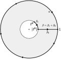
Figure 1.1. Fundamental region of $\mathbb{C}^{*}/t^{k\mathbb{Z}}$

The other cycle $\beta$ is depicted in Figure 1.1. We write $t=re^{i\psi}$. Splitting $\beta$ in an angular part $\beta_{1}$ and a radial part $\beta_{2}$, we compute

(1.2) $$\int_{\beta}\Omega=\int_{\beta_{1}}\Omega+\int_{\beta_{2}}\Omega=\int^{0}_{k\psi}e^{-i\theta}ie^{i\theta}d\theta+\int_{r^{k}}^{1}r^{-1}dr=-ik\psi-k\ln r=-\log t^{k}.$$

The canonical coordinate is given as

$$\exp\left(-2\pi i\frac{\int_{\beta}\Omega}{\int_{\alpha}\Omega}\right)=t^{k}.$$

For the purpose of generalizing this computation to higher dimensional Calabi-Yau manifolds that are not necessarily complex tori, we next recompute $\int_{\beta}\Omega$ somewhat differently. In terms of the Tate family, this means that we focus our attention on the (yet missing) central fibre. The family can be completed over the origin by an $I_{1}^{k}$ type nodal rational curve as follows. (An $I_{k}$ fibre is also possible, cf. [DR73, §VII].) Consider the action of the group $\mu_{k}$ of $k$th roots of unity on $\mathbb{A}^{2}$ given by $\zeta.(x,y)=(\zeta x,\zeta^{-1}y)$. Let $U$ be the open subspace of the quotient

$$\mathbb{A}^{2}/\mu_{k}=\operatorname{Spec}\mathbb{C}[x^{k},y^{k},xy]=\operatorname{Spec}\mathbb{C}[z,w,t]/(zw-t^{k}).$$

defined by $|t|<1$. Set $V=(\mathbb{A}^{1}\setminus\{0\})\times\{t\in\mathbb{C}\,|\,|t|<1\}\subset\mathbb{A}^{1}\setminus\{\}\times\mathbb{A}^{1}$. Define $\mathcal{X}$ to be the quotient in the analytic category defined by the étale equivalence relation (pushout)

The map $f:U\to\mathbb{A}^{1},\ (z,w,t)\mapsto t$ descends to $\mathcal{X}$. Define $X_{t}=f^{-1}(t)$. For $t\neq 0$ fixed, we find $X_{t}$ is the hypersurface of $U$ given by $z=t^{k}w^{-1}$ modulo the equivalence relation $w^{-1}=z$. So indeed $X_{t}=E_{t}$ and $\mathcal{X}_{\mathbb{D}}=f^{-1}(\mathbb{D})$ is a completion of the Tate family over the origin. By abuse of notation, we will set $\mathcal{X}=\mathcal{X}_{\mathbb{D}}$ now.

We next turn to the form to integrate. For this we choose a generator $\Omega$ of the trivial bundle $\Omega^{1}_{\mathcal{X}/\mathbb{D}}(\log X_{0})\cong\mathcal{O}_{\mathcal{X}}$. There is a canonical generator (up to sign) as before. Namely on $X_{0}$, take $\Omega|_{X_{0}}=\frac{dz}{z}=-\frac{dw}{w}$ and lift this by setting $\Omega=\frac{dz}{z}$, now on $\mathcal{X}$. The restriction of $\Omega$ to $X_{t}$ for $t\neq 0$ coincides with the $\Omega$ considered above when we computed the periods. The cycle $\alpha$ is now identified with the vanishing $1$-cycle of the degeneration of $X_{t}$ as $t\to 0$. There is only one such integral also when we go to dimension $n$ where $\alpha$ is then homeomorphic to $(S^{1})^{n}$. More interesting is the period integral over $\beta$ of which there might be several in higher dimensions. What we are going to do is construct first a tropical version $\beta_{\operatorname{trop}}$ of $\beta$ in the intersection complex of $X_{0}$. For the present degeneration of elliptic curves, degree one polarized, the intersection complex of $X_{0}$ is $B=\mathbb{R}/\mathbb{Z}$ (the moment polytope of $(\mathbb{P}^{1},\mathcal{O}(1))$ glued at its endpoints). We take $\beta_{\operatorname{trop}}=B$. Consider the moment map

$$\mathbb{P}^{1}\longrightarrow[0,1],\quad(z:w)\longmapsto\frac{|z|^{2}}{|z|^{2}+|w|^{2}}$$

Identifying endpoints in source and target respectively gives a continuous map $\pi:X_{0}\to B$ sending the node to $\{0\}$. The fibres away from $\{0\}$ are circles. Let $\beta_{0}\subset X_{0}$ be the lift of $\beta_{{\operatorname{trop}}}$ to $X_{0}$, i.e. a section of $\pi$ that maps to the non-negative real locus $\{(s:t)\mid s,t\in\mathbb{R}_{\geq 0}\}\subset\mathbb{P}^{1}$. We want to lift $\beta_{0}$ further to the nearby fibres $X_{t}$ under a retraction map $r_{t}:X_{t}\subset\mathcal{X}\to X_{0}$ to a cycle $\beta$ (in our current example $\beta$ is going to be homeomorphic to $\beta_{0}$). Restricting $\pi\circ r_{t}$ to $\beta$, defines a projection $\pi_{\beta}:\beta\to\beta_{\operatorname{trop}}$ (here a homeomorphism). We then compute the function $g(t)=\int_{\beta}\Omega$ on $\mathbb{D}$ by patching $\beta$ via various open charts $\pi_{\beta}^{-1}(W)$, $W\in\mathcal{W}$, with $W\subset\beta_{\operatorname{trop}}$ such that $g(t)$ decomposes as a sum of holomorphic functions

$$g(t)=\sum_{W\in\mathcal{W}}g_{W}(t),\quad\qquad g_{W}(t)=\int_{\pi_{\beta}^{-1}(W)\cap\beta}\Omega.$$

Since $f$ is smooth along $X_{0}$ away from the node, there exist $0<\varepsilon,\varepsilon^{\prime}<1$ so that for

$$V_{1}=\{(z,w)\in\mathbb{P}^{1}\mid\varepsilon<\frac{z}{w}<\varepsilon^{\prime}{}^{-1}\}=\pi^{-1}(W_{1}),\qquad W_{1}=\left(\frac{\varepsilon^{2}}{\varepsilon^{2}+1},\frac{1}{1+(\varepsilon^{\prime})^{2}}\right)$$

and a smaller disk $\mathbb{D}^{\prime}\subset\mathbb{D}$ we find an embedding of $U_{1}:=V_{1}\times\mathbb{D}^{\prime}$ in $\mathcal{X}$ such that $f|_{V_{1}\times\mathbb{D}^{\prime}}:V_{1}\times\mathbb{D}^{\prime}\longrightarrow\mathbb{D}^{\prime}$ is the second projection and we may assume (by modifying the embedding if necessary) that the retraction is the first projection $r:V_{1}\times\mathbb{D}^{\prime}\to V_{1}$. Let $\hat{\varepsilon}^{\prime},\hat{\varepsilon}^{\prime}{}^{-1}\in\mathbb{R}_{>0}$ denote the two points of intersection of $\beta_{0}$ with the boundary of $V_{1}$. We have that

$$g_{1}(t)=\int_{\beta\cap(\pi\circ r_{t})^{-1}(W_{1})}\Omega=\int_{\hat{\varepsilon}}^{\hat{\varepsilon}^{\prime}{}^{-1}}\frac{du}{u}=-\log{\hat{\varepsilon}^{\prime}}-\log{\hat{\varepsilon}}$$

does not depend on $t$. We set

$$U_{2}=\{(z,w,t)\in U\mid|z|<\varepsilon,|w|<\varepsilon^{\prime}\}$$

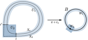
Figure 1.2. The covering of the degeneration of the Tate curve that is used to decompose the period integral, pand the rojection to the intersection complex $B$

Let $r:U_{2}\to V_{2}:=\tilde{W}_{2}\cap X_{0}$ be a retraction that coincides at the ends $|z|=\varepsilon$ and $|w|=\varepsilon^{\prime}$ with the retraction induced from $U_{1}\to V_{1}$. Let $r_{t}$ be its restriction to $X_{t}\cap U_{2}$. We compute

$$g_{2}(t)=\int_{r_{t}^{-1}(\beta_{0})}\Omega=\int^{\hat{\varepsilon}}_{{\hat{\varepsilon}^{\prime}{}^{-1}}t^{k}}\frac{dz}{z}=\log{\hat{\varepsilon}^{\prime}}+\log{\hat{\varepsilon}}-\log t^{k}$$

where we used $z=w^{-1}t^{k}$. We conclude

$$g(t)=g_{1}(t)+g_{2}(t)=-\log t^{k}$$

which coincides with (1.2). The patching method is certainly unnecessarily complicated for the Tate curve but it illustrates the approach that will generalize to higher dimensions.

While the Tate curve demonstrates some key features of our period calculation already, there are the following aspects that we additionally need to consider in higher dimensions.

1. The local model at a singular point of $X_{0}$ met by $\beta_{0}$ more generally takes the shape

   $$zw=ft^{\kappa}.$$

   We show that $f$ basically can be assumed to equal $1$ as it does not contribute to $\int_{\beta}\Omega$. This is remarkable because the so-called slab functions $f$ are known to carry enumerative information [GHK],[GS14],[La]. As our proof shows, it is precisely the normalization condition that determines the relevant enumerative corrections necessary to make the mirror map trivial. We certainly expect $f$ to enter the calculation of periods of higher weight.

2. While the tropical cycle in the dual intersection complex $\beta_{{\operatorname{trop}}}\subset B$ remains one-dimensional, its lift to $X_{t}$ will be $n$-dimensional for $n=\dim X_{t}$. The projection $\pi_{\beta}=(\pi\circ r)|_{\beta}:\beta\to\beta_{{\operatorname{trop}}}$ will generically be a $T^{n-1}=(S^{1})^{n-1}$ fibration. In order to pick $T^{n-1}$ among various choices in the fibres of $\pi\circ r$, we decorate $\beta_{\operatorname{trop}}$ with a section $\xi$ of the local system of integral flat tangent vectors $\Lambda$ on the smooth part of $B$, see Definition 0.2.

3. The tropical $1$-cycle $\beta_{{\operatorname{trop}}}$ will typically have tropical features, i.e. it is not necessarily just an $S^{1}$ as above but may bifurcate satisfying a balancing condition (0.1).

4. Some effort is necessary to show that the cycles coming from tropical $1$-cycles generate all cycles in the graded piece of the monodromy weight filtration responsible for the flat coordinates, see Corollary 5.5. Besides what is said there, we prove a general homology-cohomology comparison theorem for (co-)homology with coefficients in a constructible sheaf in §6.2 as well as a comparison of simplicial and usual sheaf homology in §6.1. Theorem 0.8 is essentially a corollary of this.

2. Analytic extensions and general setup

2.1. Analytic extensions in the compact case

The canonical smoothing obtained from [GS11] is a formal family $X$ over $\operatorname{Spec}\mathbb{C}\llbracket t\rrbracket$. Since the periods $g_{\beta}=\int_{\beta}\Omega$ have essential singularities at $0$, a word is due on how we compute these using the finite order thickenings $X_{k}$ of $X_{0}$. If $X_{0}$ is non-compact, we need to make the assumption that for any $k$ there is an analytic space $\mathcal{X}$ with a holomorphic map to a disc $T$ such that its base change to $\operatorname{Spec}\mathbb{C}[t]/t^{k+1}$ is isomorphic to $X_{k}$. We call such an $\mathcal{X}\to T$ an analytic extension of $X_{k}$. If $X_{0}$ is compact, an analytic extension of $X_{k}$ is obtained from the following result.

Theorem 2.1.

([Do74, Théorème principal, p.598]; [Gr74, Hauptsatz, p.140]) Let $X_{0}$ be a compact complex-analytic space. Then there exists a proper and flat map $\pi:\tilde{\mathcal{X}}\to S$ of complex-analytic spaces and a point $O\in S$ together with an isomorphism $\pi^{-1}(O)\simeq X_{0}$ such that $\pi$ is versal at $O$ in the category of complex analytic spaces.

Indeed, by Theorem 2.1 the formal family $\varinjlim X_{k}$ is obtained by pull-back of the versal deformation $\tilde{\mathcal{X}}\to S$ of $X_{0}$ by a formal arc in $S$. Such a formal arc can be approximated to arbitrarily high order by a map from a holomorphic disc $T$ to $S$, and $\mathcal{X}\to T$ is then defined by pull-back of the versal family.

By the definition of $\Omega$, $\int_{\alpha}\Omega$ is constant on $T$. Furthermore,

$$h_{\beta}=\exp\left(-2\pi i\frac{\int_{\beta}\Omega}{\int_{\alpha}\Omega}\right)$$

is going to be a holomorphic function on $T$, so $h_{\beta}$ is determined by its power series expansion at $0$. The Taylor series of this function up to order $k$ is determined by $X_{k}$ and hence does not depend on the choice of $\mathcal{X}$. This is true for any $k$, so we obtain in this way the entire Taylor series of $h_{\beta}$ at $0$ independent of the choices of $\mathcal{X}$. We will see that this is the Taylor series of a holomorphic function.

Furthermore, for each $k$ and each analytic extension $\mathcal{X}$ of $X_{k}$, we will consider a collection $\mathcal{U}$ of pairwise disjoint open sets in $\mathcal{X}$ whose closures cover $\mathcal{X}$ with zero measure boundary. We then decompose

$$h_{\beta}=\prod_{U\in\mathcal{U}}h_{U}$$

where $h_{U}=\exp\big{(}-2\pi i\frac{\int_{\beta\cap U}\Omega}{\int_{\alpha}\Omega}\big{)}$. We will choose the open sets such that $h_{U}$ is holomorphic for each $U\in\mathcal{U}$. Let $U_{k}$ denote the base change of $U$ to $\operatorname{Spec}\mathbb{C}[t]/t^{k+1}$. Also, the $k$th $t$-order cut-off $h^{k}_{\beta}$ of $h_{\beta}$ decomposes $h^{k}_{\beta}=\prod_{U}h^{k}_{U}$ in the $k$th order cut-offs $h^{k}_{U}$ of the $h_{U}$. Hence we can compute each $h^{k}_{\beta}$ from an open cover like $\mathcal{U}$.

We next remind ourselves of the relevant notions developed in [GS06, GS11].

2.2. Toric degenerations and log CY spaces

The full definition of a toric degeneration can be found in [GS11, Definition 1.8]. Most importantly, it is a flat morphism $f:\mathcal{X}\to T$ with the following properties:

1. $\mathcal{X}$ is normal,

2. $T=\operatorname{Spec}R$ for $R$ a discrete valuation $\mathbb{C}\llbracket t\rrbracket$-algebra,

3. the normalization $\tilde{X}_{0}$ of the central fibre $X_{0}$ is a union of toric varieties glued torically along boundary strata such that

4. away from a locus $\mathcal{Z}\subset\mathcal{X}$ of relative codimension two, the triple $(\mathcal{X},X_{0},f)$ is locally given by $(U,V,z^{\rho})$ with $U$ an affine toric variety with reduced toric divisor $V$ cut out by a monomial $z^{\rho}$,

5. $\mathcal{Z}$ is required not to contain any toric strata of $X_{0}$,

6. the normalization $\tilde{X}_{0}\to X_{0}$ is required to be $2:1$ on the union of the toric divisors of $X_{0}$ except for a divisor $\tilde{D}\subset\tilde{X}_{0}$ where it may be generically $1:1$,

7. denoting by $D$ the image of $\tilde{D}$ in $X_{0}$, the local model $(U,V,z^{\rho})$ at a point of $D\setminus\mathcal{Z}$ can be chosen so that $D$ is defined by $(z^{\rho_{D}},z^{\rho})$ for $z^{\rho_{D}}$ another monomial,

8. the components of $X_{0}$ are algebraically convex, i.e. they admit a proper map to an affine variety.

One similarly defines a formal toric degeneration as a family over $\operatorname{Spf}\mathbb{C}\llbracket t\rrbracket$. A polarization of a toric degeneration is a fibre-wise ample line bundle. At a generic point $\eta_{\tau}$ of a stratum $X_{\tau}$ of $X_{0}$, let $P_{\tau}$ denote the toric monoid such that

(2.1) $$U=\operatorname{Spec}\mathbb{C}[P_{\tau}]$$

for $(U,V,z^{\rho})$ the local model at $\eta_{\tau}$ (which exists because $\mathcal{Z}$ does not contain $\eta_{\tau}$ by (5)). One finds that $P_{\tau}$ is unique if one requires $\rho$ (respectively $\rho+\rho_{D}$ at a point in $D$) to be contained in its relative interior of $P_{\tau}$ which we assume from now on. Even though we do not use any log geometry in this paper, we should mention that the data of the local models $(U,V,z^{\rho})$ can be elegantly encoded in a log structure on $X_{0}$. This is a sheaf of monoids $\mathcal{M}_{X_{0}}$ on $X_{0}$ together with a map of monoids $\alpha:\mathcal{M}_{X_{0}}\to\mathcal{O}_{X_{0}}$ using the multiplication on $\mathcal{O}_{X_{0}}$. It is required that the structure map $\alpha$ induces an isomorphism $\alpha^{-1}(\mathcal{O}_{X_{0}}^{\times})\to\mathcal{O}_{X_{0}}^{\times}$. The way in which $\mathcal{M}_{X_{0}}$ encodes the local models is then

(2.2) $$\mathcal{M}_{{X_{0}},\eta_{\tau}}/\alpha^{-1}(\mathcal{O}_{{X_{0}},\eta_{\tau}}^{\times})\oplus\mathbb{Z}^{\dim\tau}\cong P_{\tau}$$

at the generic point $\eta_{\tau}$ of the stratum $X_{\tau}$ not contained in $D$ and there is a similar relation on $D$. The isomorphism (2.2) is not canonical unless $\dim\tau=0$. Also the monomial $z^{\rho}$ is encoded in the log structure as it is part of the data of the log morphism from $X_{0}$ to the standard log point. One defines a toric log CY-pair to be a space $X_{0}$ with log structure $\mathcal{M}_{X_{0}}$ satisfying a list of criteria that is induced by the list above on the central fibre $X_{0}$, see [GS11, Definition 1.6].

2.3. Intersection complex

We recall [GS06, §4.2]. Let $X_{0}$ denote the central fibre of a polarized toric degeneration (in fact a pre-polarization suffices, see [GS11, Ex. 1.13]). By affine convexity and the polarization, each irreducible component of $X_{0}$ is a toric variety $X_{\sigma}$ given by a lattice polyhedron $\sigma$. We glue two maximal polyhedra $\sigma_{1},\sigma_{2}$ along a facet $\tau$ if $\tau$ corresponds to a divisor in the intersection of $X_{\sigma_{1}}$ and $X_{\sigma_{2}}$. The resulting space $B$ of all such gluings is a topological manifold. Let $\mathscr{P}$ denote the set of polyhedra and their faces modulo identifications by gluing. To each cell $\tau\in\mathscr{P}$ corresponds a stratum $X_{\tau}$ of $X_{0}$ and this association is compatible with inclusions and dimensions ($\dim\tau=\dim X_{\tau}$). We will denote by $\mathscr{P}^{[k]}$ the subset of $k$-dimensional faces and by abuse of notation sometimes also their union in $B$. Since $\mathcal{Z}$ does not contain any toric strata, at the generic point of a stratum $X_{\tau}$ of $X_{0}$ there is a toric local model $(U,V,z^{\rho})$ and $U=\operatorname{Spec}\mathbb{C}[P_{\tau}]$ with $\rho\in P_{\tau}$. The monoid $P_{\tau}$ embeds in its associated group $P_{\tau}^{\operatorname{gp}}\cong\mathbb{Z}^{n+1}$. Let $P_{\tau,\mathbb{R}}$ denote the convex hull of $P_{\tau}$ in $P_{\tau,\mathbb{R}}^{\operatorname{gp}}=P_{\tau}^{\operatorname{gp}}\otimes_{\mathbb{Z}}\mathbb{R}$. Let now $\tau=v$ be a vertex. If $X_{\sigma_{1}},\ldots,X_{\sigma_{r}}$ are the $n$-dimensional strata containing the point $X_{v}$ then $\sigma_{1},\ldots,\sigma_{r}$ correspond to facets of $P_{v,\mathbb{R}}$. The composition of the embedding of the facets with the projection

(2.3) $$P_{v,\mathbb{R}}\longrightarrow P^{\operatorname{gp}}_{v,\mathbb{R}}/\mathbb{R}\rho\cong\mathbb{R}^{n}$$

provides a chart of the topological manifold $B$ in a neighbourhood of $v$. Together with the relative interiors of the maximal cells of $\mathscr{P}$, the charts provide an integral affine structure on $B$ away from a codimension two locus $\Delta$. Thus there is an atlas for $B\setminus\Delta$ with transition functions in $\operatorname{GL}_{n}(\mathbb{Z})\ltimes\mathbb{Z}^{n}$. The singular locus $\Delta$ can be chosen to be contained in the union of those simplices in the barycentric subdivision of $\mathscr{P}$ that do not contain a vertex or barycenter of a maximal cell, see [GS06, Remark 1.49]. The pair $(B,\mathscr{P})$ is called the intersection complex of $X_{0}$ (or of $\mathcal{X}$). The local models $(P_{\tau},\rho)$ provide an additional datum not yet captured in $(B,\mathscr{P})$. This is a strictly convex multivalued piecewise affine function $\varphi$ on $B$, that is, a collection of continuous functions on an open cover of $B$ that are strictly convex with respect to the polyhedral decomposition $\mathscr{P}$ and which differ by affine functions on overlaps. In particular, there is a piecewise linear representative $\varphi_{v}$ in a neighbourhood of each vertex on $\mathscr{P}$. Let $P_{v,\mathbb{R}}\cong\Lambda_{v,\mathbb{R}}\oplus\mathbb{R}\rho$ be a splitting coming from an integral section of (2.3). Then the boundary $\partial P_{v,\mathbb{R}}$ of $P_{v,\mathbb{R}}$ gives the graph of a piecewise linear function

$$\varphi_{v}:\Lambda_{v,\mathbb{R}}\longrightarrow\mathbb{R}\rho,$$

uniquely defined up to adding a linear function (change of splitting). If $v\in\partial B$, then $\varphi_{v}$ is in fact defined only on part of $\Lambda_{v}$. The collection of $P_{v}$ determines $\varphi$ completely via the collection of $\varphi_{v}$. Conversely, we can obtain all $P_{v}$ from knowing $\varphi$ via

$$P_{v}=\{(m,a)\in\Lambda_{v}\oplus\mathbb{Z}\mid\varphi_{v}(m)\leq a\}$$

where we identified $\rho=(0,1)$. The triple $(B,\mathscr{P},\varphi)$ is called a polarized tropical manifold. The local model $P_{\tau}$ for $\tau\in\mathscr{P}$ is a localization in a face corresponding to $\tau$ of the monoid $P_{v}$ for any $v\in\tau$.

2.4. Simplicity

The intersection complex $(B,\mathscr{P})$ or simply the affine manifold $B$ is called simple if certain polytopes constructed locally from the monodromy around $\Delta$ are elementary lattice simplices. This condition should be viewed as a local rigidity statement. For the precise definition, see [GS06, Definition 1.60]. It is believed that under suitable conditions, starting with an intersection complex $(B,\mathscr{P},\varphi)$ one can subdivide it to turn it into a simple $(B,\mathscr{P})$. Geometrically, this would correspond to a further degeneration of $X_{0}$. This was shown to be true for all toric degenerations arising from Batyrev-Borisov examples [Gr05]. Mumford’s degenerations of abelian varieties are automatically simple since $\Delta=\emptyset$ in this case. Hence, simplicity is a reasonable condition. We made use of it in Corollary 5.5.

2.5. Gluing data and reconstruction

By the main result of [GS11], any toric log CY space $X_{0}^{\dagger}$ with simple dual intersection complex is the central fibre of a formal toric degeneration $f:\mathcal{X}\to\operatorname{Spf}\mathbb{C}\llbracket t\rrbracket$. Furthermore, given $X_{0}^{\dagger}$ there is a canonical such toric degeneration. One constructs this order by order, so for any $k$, a map $f_{k}:X_{k}\to\operatorname{Spec}\mathbb{C}[t]/t^{k+1}$ is built such that the collection of these is compatible under restriction. We follow [GHKS, §2.2, §5.2]. Let $X^{\circ}_{0}$ denote the complement of all codimension two strata in $X_{0}$. It suffices to produce a smoothing of $X^{\circ}_{0}$ by a similar collection of finite order thickenings $X^{\circ}_{k}$, see [GHKS]. We can cover $X^{\circ}_{0}$ with two kinds of charts, $U_{\sigma}$ for $\sigma\in\mathscr{P}$ a maximal cell and $U_{\rho}$ with $\rho\in\mathscr{P}$ of codimension one. For a maximal cell $\sigma\in\mathscr{P}$, we denote by $\Lambda_{\sigma}$ the stalk of $\Lambda$ at a point in the relative interior of $\sigma$ (any two choices are canonically identified by parallel transport). For a codimension one cell $\rho\in\mathscr{P}^{[n-1]}$, we denote by $\Lambda_{\rho}$ the tangent lattice to $\rho$. This is invariant under local monodromy and thus also independent of a stalk of $\Lambda$ in $\operatorname{Int}\rho$. The two types of open sets are now given by $U_{\sigma}=\operatorname{Spec}\mathbb{C}[\Lambda_{\sigma}]$ and $U_{\rho}=\operatorname{Spec}\mathbb{C}[\Lambda_{\rho}][Z_{+},Z_{-}]/(Z_{+}Z_{-})$ for $\sigma\in\mathscr{P}^{[n]}$ and $\rho\in\mathscr{P}^{[n-1]}$ respectively. We will give the transitions for these and simultaneously that for their $k$th order thickenings. We fix a maximal cell $\sigma=\sigma(\rho)$ for each $\rho\in\mathscr{P}^{[n-1]}$. We also fix a tangent vector $w=w(\rho)\in\Lambda_{\sigma}$ such that

$$\Lambda_{\sigma}=\Lambda_{\rho}+\mathbb{Z}w.$$

So $w$ projects to a generator of $\Lambda_{\sigma}/\Lambda_{\rho}\cong\mathbb{Z}$ and we choose it so that it points from $\rho$ into $\sigma$. Assume we are given for each $\underline{\rho}\in\tilde{\mathscr{P}}^{[n-1]}$ a polynomial $f_{\underline{\rho}}\in\mathbb{C}[\Lambda_{\rho}]$ with the following compatibility property. Let $\sigma^{\prime}$ denote the other maximal cell besides $\sigma$ that contains $\rho$. Let $\underline{\rho},\underline{\rho}^{\prime}\in\tilde{\mathscr{P}}^{[n-1]}$ be both contained in $\rho\in\mathscr{P}^{[n-1]}$. The monodromy along a loop that starts in $\sigma$, passes via $\underline{\rho}$ into $\sigma^{\prime}$ and via $\underline{\rho}^{\prime}$ back into $\sigma$ is given by an automorphism of $\Lambda_{\sigma}$ that fixes $\Lambda_{\rho}$ and maps

$$w\longmapsto w+m_{\underline{\rho}\underline{\rho}^{\prime}}$$

for some $m_{\underline{\rho}\underline{\rho}^{\prime}}\in\Lambda_{\rho}$. The required compatibility between $f_{\underline{\rho}}$ and $f_{\underline{\rho}^{\prime}}$ is then

(2.4) $$t^{\kappa_{\underline{\rho}}}f_{\underline{\rho}}=z^{m_{\underline{\rho}\underline{\rho}^{\prime}}}t^{\kappa_{\underline{\rho}^{\prime}}}f_{\underline{\rho}^{\prime}}$$

so $f_{\underline{\rho}}$ determines $f_{\underline{\rho}^{\prime}}$ uniquely and vice versa. We give thickened versions of $U_{\sigma}$ and $U_{\rho}$ by giving the corresponding rings as

$$R^{k}_{\sigma}=A_{k}[\Lambda_{\sigma}],$$

$$R^{k}_{\underline{\rho}}=A_{k}[\Lambda_{\rho}][Z_{+},Z_{-}]/(Z_{+}Z_{-}-f_{\underline{\rho}}\cdot t^{\kappa_{\underline{\rho}}})$$

for $A_{k}=\mathbb{C}[t]/t^{k+1}$. When $k$ is fixed, we also write $R_{\sigma}$ for $R^{k}_{\sigma}$ and so forth. For $\sigma=\sigma(\rho)$, the map

$$\chi^{\mathrm{can}}_{\underline{\rho},\sigma}:R_{\underline{\rho}}\longrightarrow R_{\sigma}$$

is isomorphic to the localization map

$$R_{\underline{\rho}}\longrightarrow(R_{\underline{\rho}})_{Z_{+}}$$

by identifying $R_{\sigma}=(R_{\underline{\rho}})_{Z_{+}}$ via $Z_{+}=z^{w}$ and elimination of $Z_{-}$ via $Z_{-}=Z_{+}^{-1}f_{\underline{\rho}}t^{\kappa_{\underline{\rho}}}$. Similarly, if $\sigma^{\prime}$ is the other maximal cell containing $\rho$ then we obtain a vector $w_{\underline{\rho}}\in\Lambda_{\sigma^{\prime}}$ by parallel transporting $w$ from $\sigma$ to $\sigma^{\prime}$ via $\underline{\rho}$. The map $R_{\underline{\rho}}\to R_{\sigma^{\prime}}$ is then given by identifying $R_{\sigma^{\prime}}=(R_{\underline{\rho}})_{Z_{-}}$ via $Z_{-}=z^{-w_{\underline{\rho}}}$ and elimination of $Z_{+}$. The compatibility condition (2.4) implies that we have canonical isomorphisms $R_{\underline{\rho}}\cong R_{\underline{\rho}^{\prime}}$ compatible with the maps to $R_{\sigma}$ and $R_{\sigma}^{\prime}$, namely $R_{\underline{\rho}}\to R_{\underline{\rho}^{\prime}}$ via

$$Z_{+}\longmapsto Z_{+},$$

$$Z_{-}\longmapsto Z_{-}z^{m_{\underline{\rho}\underline{\rho}^{\prime}}}.$$

Definition 2.2.

(Open) gluing data $(s_{\underline{\rho},\sigma})$ is a collection of homomorphisms $s_{\underline{\rho},\sigma}:\Lambda_{\sigma}\to A_{0}^{\times}$, one for each pair $\underline{\rho}\subset\sigma$.

We can twist the maps $\chi^{\mathrm{can}}_{\underline{\rho},\sigma}$ to a map $\chi_{\underline{\rho},\sigma}$ by composing $\chi^{\mathrm{can}}_{\underline{\rho},\sigma}$ with the automorphism

$$R_{\sigma}\longrightarrow R_{\sigma},\qquad z^{m}\longmapsto s_{\underline{\rho},\sigma}(m)z^{m}.$$

While it is possible to glue all charts to a scheme we want to modify the construction further before starting the gluing, cf. [GHKS, §2.3]. In order to obtain the $X_{k}$ from [GS11], we need to consider certain combinatorial data that gives the rings of the charts that glue to $X_{k}$. For the rings, this will simply be taking further copies of the $R_{\sigma}$ and $R_{\underline{\rho}}$ that we defined already but there will be new maps and the rings get modified as we need to add higher order terms to the $f_{\underline{\rho}}$. The combinatorial object determining $X_{k}$ is called a structure whose data we now describe. It comes with a refinement $\mathscr{P}_{k}$ of $\mathscr{P}$. The maximal cells $\mathfrak{u}\in\mathscr{P}_{k}^{[n]}$ are called chambers. We denote by $\sigma_{\mathfrak{u}}\in\mathscr{P}^{[n]}$ the unique maximal cell in $\mathscr{P}$ containing $\mathfrak{u}$. The codimension one cells of $\mathscr{P}_{k}$ are called walls and are denoted $\mathfrak{p}$. A wall that is contained in $\mathscr{P}^{[n-1]}$ is called a slab and it is in fact contained in a unique $\underline{\rho}_{\mathfrak{p}}\in\tilde{\mathscr{P}}^{[n-1]}$. We typically denote slabs by $\mathfrak{b}$. A wall that is not a slab is called a proper wall and we then denote by $\sigma_{\mathfrak{p}}\in\mathscr{P}^{[n]}$ the unique maximal cell containing $\mathfrak{p}$. Each wall $\mathfrak{p}$ comes with a polynomial $f_{\mathfrak{p}}\in A_{k}[\Lambda_{\mathfrak{p}}]$ and if $\mathfrak{p}$ is a slab and $k=1$ then $f_{\mathfrak{p}}=f_{\underline{\rho}_{\mathfrak{p}}}$. If $\mathfrak{p}$ is a proper wall then

(2.5) $$f_{\mathfrak{p}}\equiv 1\mod t,$$

so $f_{\mathfrak{p}}$ is invertible.

The rings that give the charts to glue to $X_{k}^{\circ}$ are then derived from the known rings by

(2.6) $$R^{k}_{\mathfrak{u}} :=R^{k}_{\sigma_{\mathfrak{u}}}=A_{k}[\Lambda_{\sigma_{\mathfrak{u}}}] \qquad\hbox{ for a chamber }\mathfrak{u},$$

(2.7) $$R^{k}_{\mathfrak{p}} :=R^{k}_{\sigma_{\mathfrak{p}}}=A_{k}[\Lambda_{\sigma_{\mathfrak{p}}}] \qquad\hbox{ for a proper wall }\mathfrak{p},$$

(2.8) $$R^{k}_{\mathfrak{b}} :=A_{k}[\Lambda_{\mathfrak{b}}][Z_{+},Z_{-}]/(Z_{+}Z_{-}-f_{\mathfrak{b}}\cdot t^{\kappa_{\underline{\rho}_{\mathfrak{b}}}}) \qquad\hbox{ for a slab }\mathfrak{b}.$$

Once $k$ is fixed, we will write $R_{\mathfrak{u}}$ for $R^{k}_{\mathfrak{u}}$ and so forth. For every pair of a slab $\mathfrak{b}$ contained in a chamber $\mathfrak{u}$ we have a map

$$\chi_{\mathfrak{b},\mathfrak{u}}:R_{\mathfrak{b}}\longrightarrow R_{\mathfrak{u}}$$

defined just like $\chi_{\underline{\rho},\sigma}$; in particular, $\chi_{\mathfrak{b},\mathfrak{u}}$ incorporates the twist by the gluing automorphism

$$s_{\underline{\rho}_{\mathfrak{b}},\sigma_{\mathfrak{u}}}:\Lambda_{\mathfrak{u}}\longrightarrow A_{0}^{\times}.$$

Furthermore, when $\mathfrak{u},\mathfrak{u}^{\prime}$ are two chambers joined by a proper wall $\mathfrak{p}$, we have an isomorphism

$$\theta_{\mathfrak{p}}:R_{\mathfrak{u}}\longrightarrow R_{\mathfrak{u}^{\prime}},\qquad z^{m}\longmapsto f_{\mathfrak{p}}^{\langle d_{\mathfrak{p}},m\rangle}z^{m}$$

where $d_{\mathfrak{p}}$ is the generator of $\Lambda_{\mathfrak{p}}^{\perp}\subset\check{\Lambda}_{\sigma_{\mathfrak{p}}}$ that points from $\mathfrak{p}$ into $\mathfrak{u}$.

Using these chart transitions, one glues a scheme $X^{\circ}_{k}$ for every $k$ and these are compatible with restrictions $X^{\circ}_{k}\to X^{\circ}_{k-1}$.

2.6. The normalization condition

The algorithm of [GS11] produces the $(k+1)$-structure data $\mathscr{P}_{k+1}$ and all $f_{\mathfrak{p}}$ from the analogous $k$-structure data. It is inductive in $k$ and deterministic. The $f_{\mathfrak{p}}$ will get modified by higher order terms in $t$ that are being added. Apart from a modification that comes from what is called scattering and that we do not need to go into here, there is another crucial step to guarantee canonicity which is the normalization condition. The function $f_{\mathfrak{p}}$ associated to a wall is an element of $A_{k}[\Lambda_{\mathfrak{p}}]$ with non-vanishing constant term $a\in\mathbb{C}$. If $\mathfrak{p}$ is a proper wall then $a=1$. For $\mathfrak{p}=\mathfrak{b}$ a slab we consider the condition, in a suitable completion of $A_{k}[\Lambda_{\mathfrak{p}}]$ [GS11, Construction 3.24],

(2.9) $$\log\left(\frac{f_{\mathfrak{b}}}{a}\right)=\sum_{i\geq 1}\frac{(-1)^{i+1}}{i}\left(\frac{f_{\mathfrak{p}}}{a}-1\right)^{i}\hbox{ has no monomial of the form $t^{e}$ with $1\leq e\leq k$}.$$

The condition (2.9) is called the normalization up to order $k$ and can be found in [GS11, III. Normalization of slabs]. It becomes a crucial ingredient for our main result as every $f_{\mathfrak{p}}$ in the $k$-structure is $k$-normalized by loc.cit..

3. From tropical cycles to homology cycles

We assume that $B$ is oriented. Assume that we are given a tropical cycle $\beta_{\operatorname{trop}}$ on $B$ and the data of the order $k$ structure. As explained in §2.5 from this data we can glue the scheme $X^{\circ}_{k}$. We assume $X_{k}^{\circ}$ partially compactifies to $X_{k}$, a flat deformation of $X_{0}$. This can be assured with additional consistency assumptions that come out from the construction in [GS11], or in the quasiprojective case can be formulated via theta functions [GHKS]. We furthermore assume the existence of an analytic extension $f:X\to\mathbb{D}$ of $f_{k}:X_{k}\to\operatorname{Spec}A_{k}$, as established for the compact case in §2.1. By perturbing $\beta_{\operatorname{trop}}$ if necessary, we assume that its vertices lie in the interior of the chambers of $\mathscr{P}_{k}$ and that the edges meet the walls in finitely many points in their interiors. Let $\mathcal{W}$ be a collection of disjoint open sets of

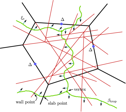
Figure 3.1. Types of points in $\beta_{\operatorname{trop}}$

$B$ such that the union of their closures covers $\beta_{\operatorname{trop}}$. We may assume that each point in $\beta_{\operatorname{trop}}$ which either is a vertex or lies in a wall of $\mathscr{P}_{k}$, is contained in a $W\in\mathcal{W}$ and each $W$ contains at most one such point. Furthermore we assume that the closures of any two open sets that contain a wall point are disjoint. We have thus four types of open sets $W\in\mathcal{W}$ given by whether it contains a vertex, slab point, wall point or none of these. For a chamber $\mathfrak{u}$, set $\sigma=\sigma_{\mathfrak{u}}$ and consider the moment map

$$\mu_{\sigma}:\operatorname{Hom}(\Lambda_{\sigma},\mathbb{C}^{\times})\to\operatorname{Int}\sigma,\qquad(z_{1},\ldots,z_{n})\longmapsto\frac{\sum_{m\in\sigma\cap\Lambda_{\sigma}}|z^{m}(z_{1},\ldots,z_{n})|^{2}\cdot m}{\sum_{m\in\sigma\cap\Lambda_{\sigma}}|z^{m}(z_{1},\ldots,z_{n})|^{2}}.$$

For the following discussion we identify $\mathbb{C}^{\times}=\mathbb{R}_{>0}\times S^{1}$ as real Lie groups, via absolute value and argument. Recall that $\mu_{\sigma}$ identifies cotangent vectors of $\sigma$ with algebraic vector fields on $\operatorname{Hom}(\Lambda_{\sigma},\mathbb{C}^{\times})\simeq(\mathbb{C}^{*})^{n}$. The induced action of $\operatorname{Hom}(\Lambda_{\sigma},S^{1})\simeq(S^{1})^{n}$ acts simply transitively on the fibres of $\mu_{\sigma}$. Moreover, there is a canonical section $S:\operatorname{Int}\sigma\to\operatorname{Hom}(\Lambda_{\sigma},\mathbb{R}_{>0})\subset\operatorname{Hom}(\Lambda_{\sigma},\mathbb{C}^{\times})$. We use this section in the interior of each chamber $\mathfrak{u}$ to lift $\beta_{\operatorname{trop}}\cap\mathfrak{u}$ to $\operatorname{Spec}\mathbb{C}[\Lambda_{\mathfrak{u}}]$. Now for an edge $e$ of $\beta_{\operatorname{trop}}$, the section $\xi_{e}\in\Gamma(e,\Lambda)$ defines a union of translates of a real $(n-1)$-torus

$$T_{e}=\{\phi\in\operatorname{Hom}(\Lambda_{\sigma},S^{1})\mid\phi(\xi_{e})=1\}\subset\operatorname{Hom}(\Gamma(e,\Lambda),S^{1})\simeq(S^{1})^{n}.$$

Note that $T_{e}$ is connected if and only if $\xi_{e}$ is primitive. Let $\bar{\xi}_{e}$ be the primitive vector such that $\xi_{e}$ is a positive multiple of $\bar{\xi}_{e}$. By assumption $\Lambda$ is oriented and $\xi_{e}$ induces an orientation of $T_{e}$, namely a basis $v_{2},\ldots,v_{n}$ of $\Lambda_{e}/\mathbb{Z}\bar{\xi}_{e}$ is oriented if $\bar{\xi}_{e},v_{2},\ldots,v_{n}$ is an oriented basis of $\Lambda_{e}$. Identifying $\Gamma(e,\Lambda)$ with $\Lambda_{\sigma}$ when $e$ passes through $\sigma$, we obtain a subgroup $T_{e}\subset\operatorname{Hom}(\Lambda_{\sigma},S^{1})$. Over the interior of a chamber $\mathfrak{u}$ we consider the orbit of the section $S$ under this torus which we denote by

$$T_{e,\mathfrak{u}}:=\operatorname{Hom}(\xi_{e}^{\perp},S^{1})\cdot S(e\cap\operatorname{Int}\mathfrak{u}).$$

Topologically $T_{e,\mathfrak{u}}$ is homeomorphic to a cylinder, a product of $(S^{1})^{n-1}$ with a closed interval. Each cylinder $T_{e,\mathfrak{u}}$ receives an orientation from the orientation of $T_{e}$ and the orientation of $e$. We wish to connect these cylinders to a cycle $\beta$ and we want to transport them to the nearby fibres.

3.1. The open cover

We construct a collection $\mathcal{U}$ of disjoint open sets of $\mathcal{X}$ whose closures will cover the lift $\beta$ of $\beta_{\operatorname{trop}}$ to all nearby fibres. The family $f:\mathcal{X}\to\mathbb{D}$ is smooth away from the codimension one strata of $X_{0}$. For each chamber $\mathfrak{u}$, we have a canonical projection $\operatorname{Spec}A_{k}[\Lambda_{\mathfrak{u}}]\to\operatorname{Spec}\mathbb{C}[\Lambda_{\mathfrak{u}}]$ and a momentum map $\mu=\mu_{\sigma_{\mathfrak{u}}}$. If $W$ is an open set entirely contained in $\mathfrak{u}$, then we include in $\mathcal{U}$ a corresponding open set $U$ whose intersection with $X_{0}$ is $\mu^{-1}(W)$ and where the family $f$ is trivialized, that is, $U=\mu^{-1}(W)\times\mathbb{D}$ and $f$ is the projection to $\mathbb{D}$. Furthermore, we may ask for the other projection $U\to\mu^{-1}(W)$ to coincide with the restriction of $\operatorname{Spec}A_{k}[\Lambda_{\mathfrak{u}}]\to\operatorname{Spec}\mathbb{C}[\Lambda_{\mathfrak{u}}]$ to the inverse image of $\mu^{-1}(W)$.

If $W$ meets a proper wall $\mathfrak{p}$ we have two chambers $\mathfrak{u}$, $\mathfrak{u}^{\prime}$ containing $\mathfrak{p}$. Again, we want $U$ to have the property that $U\cap X_{0}=\mu^{-1}(W)$. We have a trivialization $\mu^{-1}(W)\times\operatorname{Spec}A_{k}$ in the chart $\operatorname{Spec}A_{k}[\Lambda_{\mathfrak{u}}]$ and another such in the chart $\operatorname{Spec}A_{k}[\Lambda_{\mathfrak{u}^{\prime}}]$. These differ by $\theta_{\mathfrak{p}}$. We lift both trivializations from $\operatorname{Spec}A_{k}$ to $\mathbb{D}$ and take $U\subset\mathcal{X}$ to be an open set containing both of these. So we do not typically have a projection $U\to\mu^{-1}(W)$ on all of $U$. To make sure $U$ is disjoint from the previously constructed open sets, we may remove the closures of the other open sets from $U$ if necessary.

It remains to include an open set $U$ in $\mathcal{U}$ for each $W$ containing a slab point. Let $\mathfrak{b}$ be the slab and $\mathfrak{u},\mathfrak{u}^{\prime}$ be the two chambers containing it. Here we simply take any sufficiently large open set $U$ with the closure of $U\cap X_{0}$ agreeing with the closure of $\mu^{-1}(W\cap\operatorname{Int}\mathfrak{u})\cup{\mu^{\prime}}^{-1}(W\cap\operatorname{Int}\mathfrak{u}^{\prime})$. Here $\mu^{\prime}$ is the momentum map for the maximal cell containing $\mathfrak{u}^{\prime}$. To make the elements of $\mathcal{U}$ pairwise disjoint we remove the closures of the just constructed open sets that intersect the singular locus of $X_{0}$ from the previously constructed sets in $\mathcal{U}$. This way, we obtain the desired collection of open sets.

Note that except for the open sets at the slabs, there is a natural way now to transport the constructed cylinders $T_{e,\mathfrak{u}}$ to every nearby fibre $f^{-1}(t)$ for $t\in\mathbb{D}$ by taking inverse images under the projections $U\to U\cap X_{0}$. We next close the union of cylinders to an $n$-cycle $\beta$.

3.2. Closing $\beta$ at vertices

First consider the situation at a vertex $v\in\beta_{\operatorname{trop}}$. Let $\mathfrak{u}$ be the chamber containing it. We identify $\mu^{-1}(v)=\operatorname{Hom}(\Lambda_{v},S^{1}).S(v)$ with $\operatorname{Hom}(\Lambda_{v},S^{1})$. This $n$-torus contains various $(n-1)$-tori

$$T_{e,v}:=\mu^{-1}(v)\cap T_{e,\mathfrak{u}}=T_{e}\cdot S(v).$$

For each edge $e$ of $\beta_{\operatorname{trop}}$ that attaches to $v$ there is one $T_{e,v}$, and if $\xi_{e}$ is an $m_{e}$-fold multiple of a primitive vector then $T_{e,v}$ is a disjoint union of $m_{e}$ cylinders. Note that $T_{e,v}$ carries the sign $\varepsilon_{e,v}$ as the induced orientation from $T_{e,\mathfrak{u}}$. We want to show that the union of the $T_{e}\cdot S(v)$ is the boundary of an $n$-chain in the real $n$-torus $\mu^{-1}(v)$, so that we can glue them. Since the $(n-1)$-cycle $T_{e,v}$ is identified under Poincaré duality with $\varepsilon_{e,v}\xi_{e}|_{v}\in\Lambda_{v}=H^{1}(\mu^{-1}(v),\mathbb{Z})$, we see that the union of the Poincaré duals is trivial in cohomology by the balancing condition (0.1):

$$0=\sum_{v\in e}\varepsilon_{e,v}\xi_{e}.$$

Hence, the union of $T_{e,v}$ is trivial in homology and so there exists an $n$-chain $\Gamma_{v}\subset\mu^{-1}(v)$ whose boundary is this union. The chain $\Gamma_{v}$ is unique up to adding multiples of $\mu^{-1}(v)$.

3.3. Closing $\beta$ at proper walls

Let $U\in\mathcal{U}$ be an open set the corresponding open set $W\subseteq B$ of contains a point $p$ in a proper wall $\mathfrak{p}$. Let $e$ be the edge of $\beta_{\operatorname{trop}}$ containing $p$. By construction, $U$ contains $\mu^{-1}(W)\times\mathbb{D}$ in two different ways given by the trivializations in $\operatorname{Spec}A_{k}[\Lambda_{\mathfrak{u}}]$ and $\operatorname{Spec}A_{k}[\Lambda_{\mathfrak{u}^{\prime}}]$ respectively. We transport $T_{e,\mathfrak{u}}$ and $T_{e,\mathfrak{u}^{\prime}}$ into the nearby fibres by the respective trivializations. Then we need to connect theses transports over $p$. We do this by interpolation along straight real lines in $\mathbb{D}\times(\mathbb{C}^{*})^{n}\subset\mathbb{C}^{n+1}$. Let $v_{1},\ldots,v_{n}$ be an oriented basis of $\Lambda_{p}$ with $v_{1}$ pointing from $\mathfrak{p}$ into $\mathfrak{u}$ and so that $v_{2},\ldots,v_{n}$ is a basis of $\Lambda_{\mathfrak{p}}$. As before, we set $z_{j}=z^{v_{j}}$. Writing $f_{\mathfrak{p}}=1+\tilde{f}$, we have

$$\theta_{\mathfrak{p}}:\operatorname{Spec}R_{\mathfrak{u}^{\prime}}\longrightarrow\operatorname{Spec}R_{\mathfrak{u}},(t,z_{1},\ldots,z_{n})\longmapsto(t,(1+\tilde{f}(t,z_{2},\ldots,z_{n}))z_{1},z_{2},\ldots,z_{n}).$$

For fixed $x=(t,z_{1},z_{2},\ldots,z_{n})$ consider the map

$$\gamma_{x}:[0,1]\to\operatorname{Spec}R_{\mathfrak{u}},\quad\lambda\longmapsto(t,(1+\lambda\tilde{f}(t,z_{2},\ldots,z_{n}))z_{1},z_{2},\ldots,z_{n}).$$

As a map in $x$ this map extends to a neighbourhood of $U\cap X_{0}$, which we denote by the same symbol. Analogous conventions are understood at several places in the sequel. Now we define the chain $\Gamma_{p}=\bigcup_{x\in T_{e}\cdot S(p)}\gamma_{x}([0,1])$ and give it the orientation induced from that of $T_{e}$ and $[0,1]$. We find that $\Gamma_{p}$ connects $T_{e,\mathfrak{u}}$ with $T_{e,\mathfrak{u}^{\prime}}$ over $p$ with the correct orientation if $e$ traverses from $\mathfrak{u}$ to $\mathfrak{u}^{\prime}$ at $p$; otherwise we take $-\Gamma_{p}$ for this purpose.

3.4. Closing $\beta$ at slabs

Let $U\in\mathcal{U}$ correspond to an open set $W\subset B$ that contains a slab point $p\in\mathfrak{b}$. Let $e$ be the edge of $\beta_{\operatorname{trop}}$ containing $p$. We know that $U$ contains

$$\operatorname{Spec}R^{k}_{\mathfrak{b}}=\operatorname{Spec}A_{k}[\Lambda_{\mathfrak{b}}][Z_{+},Z_{-}]/(Z_{+}Z_{-}-f_{\mathfrak{b}}\cdot t^{\kappa})$$

as a non-reduced closed subspace, where $\kappa=\kappa_{\underline{\rho}_{\mathfrak{b}}}$. Without restriction we may assume that $U$ is given by a hypersurface of the form $\tilde{Z}_{+}\tilde{Z}_{-}\tilde{f}_{\mathfrak{b}}t^{\kappa_{\underline{\rho}_{\mathfrak{b}}}}=0$ in an open subset of $\mathbb{C}^{n+2}$. Let $\mathfrak{u},\mathfrak{u^{\prime}}$ denote the chambers containing $\mathfrak{b}$ with $\mathfrak{u}\subset\sigma(\rho_{\mathfrak{b}})$, with $\sigma(\rho_{\mathfrak{b}})$ the chosen maximal cell containing $\rho_{\mathfrak{b}}$. So $w=w(\rho_{\mathfrak{b}})$ points into $\mathfrak{u}$ and $Z_{+}=z^{w}$. As before, let $v_{1},\ldots,v_{n}$ be an oriented basis of $\Lambda_{p}$ with $v_{1}=w$ and $v_{2},\ldots,v_{n}$ spanning $\Lambda_{\mathfrak{b}}$. Then $z_{i}=z^{v_{i}}$ and $t$ give coordinates on $U\setminus(X_{0}\cap U)$. These correspond to the trivialization of an open subset of $f:U\to\mathbb{D}$ given by $\mathfrak{u}$. We obtain another set of coordinates replacing $Z_{+}$ by $Z^{-1}_{-}$ that comes from the trivialization of part of $U$ via $\mathfrak{u}^{\prime}$. As in §2.6 we write $f_{\mathfrak{b}}=a(1+\tilde{f})$ for $a\in\mathbb{C}^{\times}$ and $\tilde{f}$ having no constant term. Recall the gluing data $s_{\underline{\rho}_{\mathfrak{b}},\sigma_{\mathfrak{u}}}:\Lambda_{\mathfrak{u}}\to A_{0}^{\times}$, $s_{\mathfrak{u}^{\prime}}=s_{\underline{\rho}_{\mathfrak{b}},\sigma_{\mathfrak{u}^{\prime}}}:\Lambda_{\mathfrak{u}^{\prime}}\to A_{0}^{\times}$. We identify $\Lambda_{\mathfrak{u}^{\prime}}$ and $\Lambda_{\mathfrak{u}}$ by parallel transport through $\mathfrak{b}$ and set

$$s_{j}=s_{\underline{\rho}_{\mathfrak{b}},\sigma_{\mathfrak{u}}}(v_{j}),\qquad s_{j}^{\prime}=s_{\underline{\rho}_{\mathfrak{b}},\sigma_{\mathfrak{u}^{\prime}}}(v_{j}).$$

If $v_{1}^{*},\ldots,v_{n}^{*}$ denotes the dual basis to $v_{1},\ldots.,v_{n}$ then we have

(3.1) $$s_{\underline{\rho}_{\mathfrak{b}},\sigma_{\mathfrak{u}}}=\prod_{j=1}^{n}s_{j}^{v_{j}^{*}},\qquad s^{\prime}_{\underline{\rho}_{\mathfrak{b}},\sigma_{\mathfrak{u}^{\prime}}}=\prod_{j=1}^{n}(s^{\prime}_{j})^{v_{j}^{*}}.$$

Solving for $Z_{+}$ yields $Z_{+}=f_{\mathfrak{b}}t^{\kappa}Z_{-}^{-1}$, so the transformation on points given in the second set of coordinates to the first reads

$$\theta_{\mathfrak{b}}:(t,z_{1},\ldots,z_{n})\longmapsto\left(t,\frac{s^{\prime}_{1}}{s_{1}}a(1+\tilde{f}(t,s^{\prime}_{2}z_{2},\ldots,s^{\prime}_{n}z_{n}))t^{\kappa}z_{1},\frac{s^{\prime}_{2}}{s_{2}}z_{2},\ldots,\frac{s^{\prime}_{n}}{s_{n}}z_{n}\right).$$

We factor $\theta_{\mathfrak{b}}=\theta_{s,a}\circ\theta_{f}$ where

$$\theta_{f}:(t,z_{1},\ldots,z_{n})\longmapsto\left(t,(1+\tilde{f}(t,s_{2}z_{2},\ldots,s_{n}z_{n}))z_{1},z_{2},\ldots,z_{n}\right),$$

$$\theta_{s,a}:(t,z_{1},\ldots,z_{n})\longmapsto\left(t,\frac{s^{\prime}_{1}}{s_{1}}at^{\kappa}z_{1},\frac{s^{\prime}_{2}}{s_{2}}z_{2},\ldots,\frac{s^{\prime}_{n}}{s_{n}}z_{n}\right).$$

We have $\partial W\cap\beta_{\operatorname{trop}}=\{b,b^{\prime}\}$, say $b\in\mathfrak{u},b^{\prime}\in\mathfrak{u}^{\prime}$. Let $S:\mathfrak{u}\to\operatorname{Spec}\mathbb{C}[\Lambda_{\mathfrak{u}}]$ and $S^{\prime}:\mathfrak{u}^{\prime}\to\operatorname{Spec}\mathbb{C}[\Lambda_{\mathfrak{u}^{\prime}}]$ be the respective sections of the moment map. We have $(n-1)$-tori $T_{e}\cdot S(b)$ and $T_{e}\cdot S^{\prime}(b^{\prime})$ that we transport to the nearby fibres by the respective trivializations of $f$. We then want to connect them in each fibre of $f$. We first attach a chain $\Gamma_{b^{\prime}}$ to $T_{e}\cdot S(b)$ that we construct in a similar way as we built $\Gamma_{p}$ at a proper wall point. It takes care of the transformation $\theta_{f}$. Let $S(b)=(r_{1},\ldots,r_{n})$ and $S^{\prime}(b^{\prime})=(r^{\prime}_{1},\ldots,r^{\prime}_{n})$ be the respective coordinates. As a second step we then need to connect $T_{e}\cdot(r_{1},\ldots,r_{n})$ to $T_{e}\cdot(\frac{s^{\prime}_{1}}{s_{1}}at^{\kappa}r^{\prime}_{1},\frac{s^{\prime}_{2}}{s_{2}}r^{\prime}_{2},\ldots,\frac{s^{\prime}_{n}}{s_{n}}r^{\prime}_{n})$ which we do by straight line interpolation. Let $\log$ denote the inverse of $\exp$ with imaginary part in $[0,2\pi)$. For $\lambda\in[0,1]$ and $z\in\mathbb{C}^{*}$, we set $z^{\lambda}:=\exp(\lambda\log(z))$. For $t\in T_{e}$ we map $[0,1]$ into $U$ by

$$\lambda\longmapsto\left(\left(\frac{s^{\prime}_{1}}{s_{1}}at^{\kappa}\frac{r_{1}^{\prime}}{r_{1}}\right)^{\lambda}r_{1},\left(\frac{s^{\prime}_{2}}{s_{2}}\frac{r_{2}^{\prime}}{r_{2}}\right)^{\lambda}r_{2},\ldots,\left(\frac{s^{\prime}_{n}}{s_{n}}\frac{r_{n}^{\prime}}{r_{n}}\right)^{\lambda}r_{n}\right).$$

Taking the $T_{e}$-orbit of the image of $[0,1]$ traces out a chain $\Gamma_{p}$ and the concatenation of $\pm\Gamma_{p}$ and $\pm\Gamma_{b^{\prime}}$ closes $\beta$ over the slab point $p$ (the sign $\pm$ being $+$ if and only if $e$ traverses from $\mathfrak{u}$ to $\mathfrak{u}^{\prime}$ at $p$).

4. Computation of the period integrals

As before, we assume $B$ to be oriented, so we have a canonical $n$-form $\Omega\in\Omega_{X_{0}^{\dagger}/0^{\dagger}}$ given by $\operatorname{dlog}z^{v_{1}}\wedge\ldots\wedge\operatorname{dlog}z^{v_{n}}$ for $v_{1},\ldots,v_{n}$ an oriented basis $\Lambda_{\sigma}$ for any maximal cell $\sigma$. The orientation of $B$ ensures $\Omega$ is independent of $\sigma$. Since $\Omega^{n}_{\mathcal{X}^{\dagger}/T^{\dagger}}\cong f^{*}\mathcal{O}_{T}$, there is a canonical extension of $\Omega$ to $\mathcal{X}$ by requiring

$$\int_{\alpha}\Omega=\operatorname{const}$$

as a function on $T$ for $\alpha\cong(S^{1})^{n}$ a vanishing $n$-cycle at a deepest point of $X_{0}$ (any two choices for $\alpha$ are homologous).

Lemma 4.1.

$\displaystyle\int_{\alpha}\Omega=(2\pi i)^{n}.$

Proof.

This can be checked in any local chart of a deepest point, so let $v\in\mathscr{P}$ be a vertex and $P_{v}$ the associated monoid such that $\mathcal{X}$ in a neighbourhood of the deepest stratum $x\in X_{0}$ corresponding to $v$ is given by $U=\operatorname{Spec}\mathbb{C}[P_{v}]$ and $f=z^{\rho}$ with $\rho\in P_{v}$. The fibre $f^{-1}(1)$ is given by

$$\{\phi\in\operatorname{Hom}(P_{v},\mathbb{C})\mid\varphi(\rho)=1\}$$

which contains the vanishing $n$-cycle as

$$\alpha=\{\phi\in\operatorname{Hom}(P_{v},S^{1})\mid\varphi(\rho)=1\}=\operatorname{Hom}(P_{v}/\rho,S^{1})$$

Note that $P_{v}/\rho=\Lambda_{v}$, so $\alpha=\operatorname{Hom}(\Lambda_{v},S^{1})$ which we can homotope to the central fibre and integrate there. Let $v_{1},\ldots,v_{n}$ be an oriented basis of $\Lambda_{v}$ then $\Omega=\operatorname{dlog}z^{v_{1}}\wedge\ldots\wedge\operatorname{dlog}z^{v_{n}}$. Set $z^{v_{j}}=r_{j}e^{i\theta_{j}}$, so $\operatorname{dlog}z^{v_{j}}=\operatorname{dlog}r_{j}+id\theta_{j}$. Since $\alpha$ is parametrized by having each $\theta_{j}\in[0,2\pi)$, we obtain

$$\int_{\alpha}\Omega=\int_{\theta_{1},\ldots,\theta_{n}}i^{n}d\theta_{1}\wedge\ldots\wedge d\theta_{n}=(2\pi i)^{n}.$$

∎

We will make use of the following simple lemma.

Lemma 4.2.

Let $0\neq\xi\in\mathbb{Z}^{n}$ and let

$$T=\{\phi\in\operatorname{Hom}(\mathbb{Z}^{n},\mathbb{R}/\mathbb{Z})\mid\phi(\xi)=0\}$$

be the possibly disconnected codimension one subgroup of $\operatorname{Hom}(\mathbb{Z}^{n},\mathbb{R}/\mathbb{Z})$. Let $\theta_{1},\ldots,\theta_{n}$ be a basis of $\mathbb{Z}^{n}$ and therefore a set of functions $\phi\mapsto\phi(\theta_{j})$ on $T$. Their duals $\theta_{1}^{*},\ldots,\theta_{n}^{*}$ are standard coordinates on $\mathbb{R}^{n}$. To give $T$ an orientation, it suffices to give it for its identity component. We define a basis $v_{2},\ldots,v_{n}$ of $T_{0}T$ to be oriented if $\xi,v_{2},\ldots,v_{n}$ is an oriented basis of $\mathbb{Z}^{n}$ for its standard orientation. We have

$$\int_{T}d\theta_{2}\ldots d\theta_{n}=\langle\theta_{1}^{*},\xi\rangle$$

and more generally

$$\int_{T}d\theta_{1}\ldots\widehat{d\theta_{j}}\ldots d\theta_{n}=(-1)^{j+1}\langle\theta_{j}^{*},\xi\rangle.$$

Proof.

The more general statement follows from the first statement by permutation and relabelling of variables. The map from $T$ to $\operatorname{span}\{\theta_{2}^{*},\ldots,\theta_{n}^{*}\}/\mathbb{Z}^{n-1}$ has degree $\langle\theta_{1}^{*},\xi\rangle$. Indeed, this map is obtained by applying $\operatorname{Hom}(\cdot,\mathbb{R}/\mathbb{Z})$ to $\oplus_{i=2}^{n}\mathbb{Z}e_{i}\to\mathbb{Z}^{n}/\xi\mathbb{Z}$ and this map has determinant $\langle\theta_{1}^{*},\xi\rangle$. ∎

The purpose of this section is to prove Theorem 0.4. When we write $\int_{\beta}\Omega$ in the following, we understand this integral as a function in $t$ for $t\neq 0$. In particular, we implicitly transport $\beta$ into all nearby fibres. The ambiguity of doing so due to monodromy will be reflected by the circumstance that the logarithm in the base coordinate appears. Without further mention, we thus implicitly choose a branch cut in the base. The choice implicitly made here is undone upon exponentiating as we eventually do to obtain $h_{\beta}$ for the assertion of Theorem 0.4.

In the coming sections we first deal with the integral of $\Omega$ over each piece of $\beta$ individually before we finally put the results together. In the computation we pretend that the patching of our $k$-th order approximation agrees with the patching of $\mathcal{X}$. The result of the period computation can, however, be expressed purely in terms of the result of applying the logarithmic deriviative $t\frac{d}{dt}$ to the period integrals and hence, to order $k$, only depends on the behaviour of the patching to the same order. Thus this presentational simplification is justified.

4.1. Integration over the wall-add-in $\Gamma_{p}$

We assume the setup and notation of §3.3. We have a parametrization of $\Gamma_{p}$ in the fibre of $f$ for fixed $t$ given by

$$\phi:(T_{e}\cdot S(p))\times[0,1]\to U,\qquad(z_{1},\ldots,z_{n},\lambda)\longmapsto(1+\lambda\tilde{f}(t,z_{2},\ldots,z_{n}))z_{1},z_{2},\ldots,z_{n})$$

Pulling back $\Omega$ under $\phi$ yields

$$\begin{array}[]{rcl}\phi^{*}\Omega&=&\Omega+\operatorname{dlog}(1+\lambda\tilde{f}(t,z_{2},\ldots,z_{n}))\wedge\operatorname{dlog}z_{2}\wedge\ldots\wedge\operatorname{dlog}z_{n}\\ &=&\Omega+\partial_{\lambda}\log(1+\lambda\tilde{f}(t,z_{2},\ldots,z_{n}))d\lambda\wedge\operatorname{dlog}z_{2}\wedge\ldots\wedge\operatorname{dlog}z_{n}.\\ \end{array}$$

As the first summand $\Omega$ is constant in $\lambda$, it is trivial as an $n$-form on $(T_{e}\cdot S(p))\times[0,1]$ and we only need to deal with the second term. Let $u_{1},\ldots,u_{n-1}$ be standard coordinates on $\mathbb{R}^{n-1}$ that we use as coordinates on $\mathbb{R}^{n-1}/\mathbb{Z}^{n-1}$. Set $z_{j}=r_{j}e^{i\theta_{j}}$ and let

$$\theta_{j}=\sum_{k=1}^{n-1}a_{k,j}u_{k}$$

for $1\leq j\leq n$ be a linear parametrization of $T_{e}$ where $u_{j}\in[0,1)$. If $S(p)=(r_{1},\ldots,r_{n})$ then we have

$$\int_{\Gamma_{p}}\Omega =\int_{(T_{e}\cdot S(p))\times[0,1]}\phi^{*}\Omega$$

$$=\int_{u_{1},\ldots,u_{n-1}}\int_{\lambda}\partial_{\lambda}\log(1+\lambda\tilde{f}(t,r_{2}e^{i\theta_{2}},\ldots,r_{n}e^{i\theta_{n}}))d\lambda\operatorname{dlog}(r_{2}e^{i\theta_{2}})\ldots\operatorname{dlog}(r_{n}e^{i\theta_{n}})$$

$$=c\int_{u_{1},\ldots,u_{n-1}}\int_{\lambda}\partial_{\lambda}\log(1+\lambda\tilde{f}(t,r_{2}e^{i\sum a_{k,2}u_{k}},\ldots,r_{n}e^{i\sum a_{k,n}u_{k}}))d\lambda du_{1}\ldots du_{n-1}$$

where $c\in\mathbb{C}$ equals $i^{n-1}$ multiplied by a polynomial expression in the $a_{k,j}$. Integrating out $\lambda$ leads to

$$\int_{\Gamma_{p}}\Omega=c\int_{u_{1},\ldots,u_{n-1}}\log(1+\tilde{f}(t,r_{2}e^{i\sum a_{k,2}u_{k}},\ldots,r_{n}e^{i\sum a_{k,n}u_{k}}))du_{1}\ldots du_{n-1}.$$

This integral vanishes up to $t$-order $k$ by the following lemma combined with the normalization condition (2.9).

Lemma 4.3.

Let $m\in\mathbb{C}[z_{1},\ldots,z_{n-1}]$ be a monomial then

$$\int_{u_{1},\ldots,u_{n-1}}m(e^{iu_{1}},\ldots,e^{iu_{n-1}})du_{1}\ldots du_{n-1}\neq 0$$

if and only if $m$ is constant.

4.2. Integration over the vertex-add-in $\Gamma_{v}$

We assume the setup and notation of §3.2. We have $\Gamma_{v}\subset\mu^{-1}(v)=\operatorname{Hom}(\Lambda_{v},S^{1})$.

Lemma 4.4.

Let $v\in\beta_{\operatorname{trop}}$ be a vertex of valency $V$. Then for an oriented basis $v_{1},\ldots,v_{n}$ of $\Lambda_{v}$ and $z^{v_{j}}=r_{j}e^{i\theta_{j}}$, we get

$$\int_{\Gamma_{v}}\Omega=i^{n}\int_{\Gamma_{v}}d\theta_{1}\ldots d\theta_{n}\in\left\{\begin{array}[]{ll}(2\pi i)^{n}\mathbb{Z}&V\hbox{ is even,}\\ (2\pi i)^{n}\frac{1}{2}\mathbb{Z}&V\hbox{ is odd.}\end{array}\right.$$

Proof.

We have $\sum_{v\in e}\varepsilon_{e,v}\xi_{e}=0$. Set $\xi_{j}:=\varepsilon_{e_{j},v}\xi_{e_{j}}$ for $e_{1},...,e_{r}$ an enumeration of the edges containing $v$.

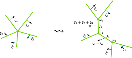
Figure 4.1. Making a vertex trivalent by the insertion of new edges

We decompose $v$ into trivalent vertices via insertion of $V-3$ new edges $f_{1},...,f_{V-3}$ meeting the existing edges in the configuration depicted in Figure 4.1. Precisely, we replace $v$ by a chain of new edges $f_{1},...,f_{V-3}$ such that the ending point of $f_{j}$ is the starting points of $f_{j+1}$. Let $w_{1},...,w_{V-2}$ denote the vertices in this chain. We arrange it so that $w_{1}$ meets $e_{1},e_{2}$, $w_{2}$ meets $e_{3}$, $w_{3}$ meets $e_{4}$ and so forth, finally $w_{V-2}$ meets $e_{V-1},e_{V}$. The edge $f_{j}$ is decorated with the section $\xi_{1}+...+\xi_{j+1}$. One checks that at each vertex $w_{j}$ the balancing condition holds. One also checks that the new tropical curve is homologous to the original one. Adding boundaries of suitable 2-cycles, we can successively slide down the edges $e_{3}$, $e_{4}$,… to $w_{1}$. In this process the sections along $f_{1},...,f_{V-3}$ get modified and when all $e_{j}$ have been moved to the first vertex, the sections of the $f_{j}$ are all trivial and so we end up in the original setup setting $w_{1}=v$. Similarly, one checks that the associated $n$-cycles to the original and modified $\beta_{\operatorname{trop}}$ are seen to be homologous. Hence

$$\int_{\Gamma_{v}}\Omega=\int_{\Gamma_{w_{1}}}\Omega+\ldots+\int_{\Gamma_{w_{V-2}}}\Omega.$$

It is not hard to see that we have reduced the assertion to the case where $v$ is trivalent. So we assume $V=3$ now. As before, set $\xi_{j}:=\varepsilon_{e_{j},v}\xi_{e_{j}}$ for $j=1,2,3$. By the balancing condition, the saturated integral span $V$ of $\xi_{1},\xi_{2},\xi_{3}$ has either rank one or two. In either case, we have a product situation where we can split $\Lambda_{v}\cong V\oplus W$ which yields a split of the torus

$$\operatorname{Hom}(\Lambda_{v},S^{1})\cong(V\otimes_{\mathbb{Z}}\mathbb{R})/V\times(W\otimes_{\mathbb{Z}}\mathbb{R})/W$$

and $\Gamma_{v}$ also splits as $\bar{\Gamma}_{v}\times(W\otimes_{\mathbb{Z}}\mathbb{R})/W$. Integration over $(W\otimes_{\mathbb{Z}}\mathbb{R})/W$ yields a factor of $(2\pi i)^{n-1}$ when $V$ is one-dimensional and $(2\pi i)^{n-2}$ when $V$ is two-dimensional. We may thus assume that $\Lambda_{v}=V$.

We do the one-dimensional case first. Let $e$ be a primitive generator of $V$ and $\xi_{j}=a_{j}e$. We have $a_{1}+a_{2}+a_{3}=0$. Now, $\Gamma_{v}$ is a union of intervals that connect the points given by $\frac{1}{a_{1}}\mathbb{Z}$, $\frac{1}{a_{2}}\mathbb{Z}$, $\frac{1}{a_{3}}\mathbb{Z}$ on $\mathbb{R}/\mathbb{Z}$. We want to show that the signed area of $\Gamma_{v}$ is $\frac{1}{2}(2\pi i)$. We may assume that $a_{1},a_{2},a_{3}$ are pairwise coprime, since the non-coprime case is a finite cover of the coprime case and the relative area of $\Gamma_{v}$ over the entire circle doesn’t change when going to the cover. So let $a_{1},a_{2},a_{3}$ be pairwise coprime. The points on the circle are then all distinct except for the origin. At the origin, we have three points with both signs appearing, so after sign cancellation, we have distinct points everywhere. The signs of the points alternate. This implies that $\Gamma_{v}$ consists of every other interval between the points. Furthermore these interval all carry the same sign. The set of points is symmetric under the involution $\iota:x\mapsto-x$. However, $\iota$ takes $\Gamma_{v}$ to its complement, so up to sign $\Gamma_{v}$ and $\iota(\Gamma_{v})$ have the same area. Since

$$2\pi i=\int_{\Gamma_{v}}d\theta+\int_{-\iota(\Gamma_{v})}d\theta,$$

we conclude that $\int_{\Gamma_{v}}d\theta=\frac{1}{2}(2\pi i)$. The case when $V$ is two-dimensional works similar. ∎

4.3. Integration over the slab-add-in $\Gamma_{v}$

We assume the setup and notation of §3.4. We filled in the two cylinders $\Gamma_{p}$ and $\Gamma_{b^{\prime}}$ at the slab. We have $\int_{\Gamma_{b^{\prime}}}\Omega=0$ by §4.1. We parametrize $\Gamma_{p}$ by $\phi:T_{e}\times[0,1]\to U$ given as

$$(e^{i\theta_{1}},\ldots,e^{i\theta_{n}},\lambda)\longmapsto\left(\left(\frac{s^{\prime}_{1}}{s_{1}}at^{\kappa}\frac{r_{1}^{\prime}}{r_{1}}\right)^{\lambda}r_{1}e^{i\theta_{1}},\left(\frac{s^{\prime}_{2}}{s_{2}}\frac{r_{2}^{\prime}}{r_{2}}\right)^{\lambda}r_{2}e^{i\theta_{2}},\ldots,\left(\frac{s^{\prime}_{n}}{s_{n}}\frac{r_{n}^{\prime}}{r_{n}}\right)^{\lambda}r_{n}e^{i\theta_{n}}\right).$$

Note that

$$\operatorname{dlog}\left(\left(\frac{s^{\prime}_{j}}{s_{j}}\frac{r_{j}^{\prime}}{r_{j}}\right)^{\lambda}r_{j}e^{i\theta_{j}}\right)=\log\left(\frac{s^{\prime}_{j}}{s_{j}}\frac{r_{j}^{\prime}}{r_{j}}\right)d\lambda+id\theta_{j}.$$

We compute

$$\begin{array}[]{rcl}\phi^{*}\Omega&=&\displaystyle\log\left(\frac{s^{\prime}_{1}}{s_{1}}at^{\kappa}\frac{r_{1}^{\prime}}{r_{1}}\right)i^{n-1}d\lambda\wedge d\theta_{2}\wedge\ldots\wedge d\theta_{n}+\ldots\\ &&+\displaystyle\log\left(\frac{s^{\prime}_{n}}{s_{n}}\frac{r_{n}^{\prime}}{r_{n}}\right)i^{n-1}d\theta_{1}\wedge\ldots\wedge d\theta_{n-1}\wedge d\lambda.\\[11.38109pt] &=&\displaystyle\log\left(at^{\kappa}\right)i^{n-1}d\lambda\wedge d\theta_{2}\wedge\ldots\wedge d\theta_{n}\\ &&+\displaystyle\sum_{j=1}^{n}(-1)^{j+1}\log\left(\frac{s^{\prime}_{j}}{s_{j}}\frac{r_{j}^{\prime}}{r_{j}}\right)i^{n-1}d\lambda\wedge d\theta_{1}\wedge\ldots\wedge\widehat{d\theta_{j}}\wedge\ldots\wedge d\theta_{n-1}.\\ \end{array}$$

Integrating out $\lambda$ and Lemma 4.2 yield

(4.1) $$\begin{array}[]{rcl}\displaystyle\int_{\Gamma_{p}}\Omega=\int_{T_{e}}\int_{\lambda}\phi^{*}\Omega&=&\displaystyle(2\pi i)^{n-1}\log\left(at^{\kappa}\right)\langle v_{1}^{*},\xi_{e}\rangle\\ &&+(2\pi i)^{n-1}\displaystyle\sum_{j=1}^{n}\log\left(\frac{s^{\prime}_{j}}{s_{j}}\frac{r_{j}^{\prime}}{r_{j}}\right)\langle v_{j}^{*},\xi_{e}\rangle.\end{array}$$

We record for later use that evaluating the logarithms, we find among the summands

(4.2) $$(2\pi i)^{n-1}\displaystyle\sum_{j=1}^{n}\log(r_{j}^{\prime})\langle v_{j}^{*},\xi_{e}\rangle\,-\,(2\pi i)^{n-1}\displaystyle\sum_{j=1}^{n}\log(r_{j})\langle v_{j}^{*},\xi_{e}\rangle.$$

Furthermore using (3.1), we find

$$\sum_{j=1}^{n}\log\left(\frac{s^{\prime}_{j}}{s_{j}}\right)\langle v_{j}^{*},\xi_{e}\rangle=\log\left(\frac{s_{\mathfrak{b},\sigma_{\mathfrak{u}^{\prime}}}(\xi)}{s_{\mathfrak{b},\sigma_{\mathfrak{u}}}(\xi)}\right).$$

As $\mathfrak{b},\mathfrak{u},\mathfrak{u^{\prime}}$ and $a$ are determined by $p$, we may shortcut

(4.3) $$s_{p}:=a\frac{s_{\rho_{\mathfrak{b}},\sigma_{\mathfrak{u}^{\prime}}}(\xi)}{s_{\rho_{\mathfrak{b}},\sigma_{\mathfrak{u}}}(\xi)}:\Lambda_{p}\longrightarrow\mathbb{C}^{*}$$

if $e$ traverses from $\mathfrak{u}$ to $\mathfrak{u}^{\prime}$ at $p$ and we define $s_{p}$ to be the inverse of (4.3) if $e$ traverses in the opposite direction.

4.4. Integration over part of an edge

Let $c$ be a connected part of an edge $e$ of $\beta$ that lies in the interior of a maximal cell $\sigma=\sigma_{\mathfrak{u}}$ of $\mathscr{P}$ and is contained in the closure of a chamber $\mathfrak{u}$. As in §4.3, we parametrize $T_{e}\cdot S(c)$ by $\phi:T_{e}\times[0,1]\to\operatorname{Spec}\mathbb{C}[\Lambda_{\sigma}]$ so that $\phi(x,[0,1])$ is co-oriented with $e$. In the coordinates $z^{v_{1}},\ldots,z^{v_{n}}$ let $(r_{1},\ldots,r_{n})$ and $(r_{1}^{\prime},\ldots,r_{n}^{\prime})$ be the starting and ending points, respectively, of the lift of $c$ under the section of the moment map. From the calculation in §4.3, by setting $s_{i}=s_{i}^{\prime}=a=1$ and $\kappa=0$, we obtain

$$\int_{T_{e}\cdot S(c)}\Omega=(2\pi i)^{n-1}\displaystyle\sum_{j=1}^{n}\log(r_{j}^{\prime})\langle v_{j}^{*},\xi_{e}\rangle\,-\,(2\pi i)^{n-1}\displaystyle\sum_{j=1}^{n}\log(r_{j})\langle v_{j}^{*},\xi_{e}\rangle.$$

4.5. Integration in a neighbourhood of a vertex

Let $W\in\mathcal{W}$ be a neighbourhood containing a vertex $v$ of $\beta$ and let $U\in\mathcal{U}$ be the corresponding open set in $\mathcal{X}$. The cycle $\beta_{U}:=\beta\cap U$ consists of the vertex-filling cycle $\Gamma_{v}$ and various cylinders $\Gamma_{c_{k}}$, $k=1,\ldots,r$ one for each edge $e_{k}$ meeting $v$. We may thus compute $\int_{\beta_{U}}\Omega$ by adding the results from §4.2 and §4.4. Say the moment map lift of $v$ has coordinates $(r_{1},\ldots,r_{n})$ and the other endpoint of the lift of $c_{k}$ is $(r^{\prime}_{1}(k),\ldots,r^{\prime}_{n}(k))$ then

$$\int_{\beta_{U}}\Omega = \int_{\Gamma_{v}}\Omega+\sum_{k=1}^{r}\int_{\Gamma_{c_{k}}}\Omega$$

$$= (2\pi i)^{n}a_{v}+(2\pi i)^{n-1}\sum_{k=1}^{r}\varepsilon_{e_{k},v}\Big{(}\sum_{j=1}^{n}\log(r^{\prime}_{j}(k))\langle v_{j}^{*},\xi_{e}\rangle-\sum_{j=1}^{n}\log(r_{j})\langle v_{j}^{*},\xi_{e}\rangle\Big{)}.$$

Using the balancing condition (0.1), this reduces to

$$\int_{\beta_{U}}\Omega=(2\pi i)^{n}a_{v}+(2\pi i)^{n-1}\sum_{k=1}^{r}\varepsilon_{e_{k},v}\sum_{j=1}^{n}\log(r^{\prime}_{j}(k))\langle v_{j}^{*},\xi_{e}\rangle.$$

4.6. Integration in the neighbourhood of a wall

Let $W\in\mathcal{W}$ be a neighbourhood containing a wall point $p$ of $\beta$ and let $U\in\mathcal{U}$ be the corresponding neighbourhood of $\mathcal{X}$. The cycle $\beta_{U}:=\beta\cap U$ consists of the wall-point-filling cycle $\Gamma_{v}$ and two cylinders $\Gamma_{c_{1}}$, $\Gamma_{c_{2}}$ for $c_{1},c_{2}\subset e$ for $e$ the edge of $\beta$ that contains $p$. Say $c_{1},c_{2}$ have the same orientation as $e$ and are ordered by the orientation as well. Since the integral over $\Gamma_{p}$ is zero by §4.1 and since the endpoint of $c_{1}$ coincides with the starting point of $c_{2}$, using §4.4 and cancellation at $p$, we obtain

$$\int_{\beta_{U}}\Omega=(2\pi i)^{n-1}\displaystyle\sum_{j=1}^{n}\log(r_{j}^{\prime})\langle v_{j}^{*},\xi_{e}\rangle\,-\,(2\pi i)^{n-1}\displaystyle\sum_{j=1}^{n}\log(r_{j})\langle v_{j}^{*},\xi_{e}\rangle.$$

with $(r_{1},\ldots,r_{n})$ the starting point of $c_{1}$ and $(r^{\prime}_{1},\ldots,r^{\prime}_{n})$ the endpoint of $c_{2}$.

4.7. Proof of Theorem 0.4

We have

$$\int_{\beta}\Omega=\sum_{U\in\mathcal{U}}\int_{\beta\cap U}\Omega.$$

We computed the summands in the previous section and just need to add the results. We show that all terms of the form

$$(2\pi i)^{n-1}\displaystyle\sum_{j=1}^{n}\log(r_{j})\langle v_{j}^{*},\xi_{e}\rangle$$

with varying $(r_{1},\ldots,r_{n})$ cancel. We claim that whenever to cylinders $\Gamma_{c_{1}}$, $\Gamma_{c_{2}}$ share an endpoint, the corresponding terms for these endpoints carry opposite sign and thus cancel. This is in fact easy to see if $c_{1},c_{2}$ lie in the same maximal cell $\sigma$ as the coordinates $z^{v_{1}},\ldots,z^{v_{n}}$ that we used to write down $(r_{1},\ldots,r_{n})$ with $v_{j}$ a basis of $\Lambda_{\sigma}$ extend to all open sets of the form $U\cap X_{0}$ with $U$ meeting no other component of $X_{0}$ than $X_{\sigma}$. It remains to take a closer look at a slab $\mathfrak{b}$ where a transition from $\Lambda_{\sigma}$ to $\Lambda_{\sigma^{\prime}}$ occurs ($\sigma\neq\sigma^{\prime}$). Here, we can identify $\Lambda_{\sigma^{\prime}}$ with ($\sigma\neq\sigma^{\prime}$) via parallel transport through $\mathfrak{b}$. Then (4.2) implies the desired cancellation there as well.

Now Theorem 0.4 directly follows up to signs. To check the signs note that $d_{p}$ in the statement of the theorem points in the opposite direction as $v_{1}^{*}$ in the definition of the slab add-in. This induces a negative sign that cancels with the negative sign in the multiplication with $-2\pi i$ in the definition of $h_{\beta}$. Hence, we are done.

5. Tropical cycles generate all cycles

Theorem 5.1.

Let $(B,\mathscr{P})$ be an oriented tropical manifold. We have

(5.1) $$H^{n-1}(B,i_{*}\Lambda) =H_{1}(B,\partial B;i_{*}\Lambda)$$

(5.2) $$H_{1}(B,\partial B;i_{*}\Lambda) =H_{1}^{\mathscr{P}^{{\operatorname{bar}}}}(B,\partial B;i_{*}\Lambda)$$

Proof.

(5.1) is Theorem 6.9 and (5.2) is Theorem 6.4. ∎

Theorem 5.2.

Let $(B,\mathscr{P})$ be a tropical manifold. Any element in $H_{1}(B,\partial B;i_{*}\Lambda)$ can be represented by a tropical $1$-cycle.

Proof.

By Theorem 5.1, (2) we are dealing with an element of $H_{1}^{\mathscr{P}^{{\operatorname{bar}}}}(B,\partial B;i_{*}\Lambda)$ which is a similar object as a tropical $1$-cycle. However, its vertices are the barycenters of $B$. We can ignore edges in $\partial B$. We perturb the vertices by adding the boundary of a $2$-chain of $H_{1}(B,\partial B;i_{*}\Lambda)$ so that the vertices that were in $\partial B$ stay in $\partial B$ and become univalent and the vertices in the interior of $B$ all move into the maximal cells of $B$ so that the new edges between them do not meet $\Delta$. ∎

For a treatment of to log-differential forms in our setup, see [GS10]. In short, let $\mathcal{Z}$ denote the locus in $\mathcal{X}$ where $f$ is log-singular and $j:\mathcal{X}\setminus\mathcal{Z}\hookrightarrow\mathcal{X}$ the inclusion of its complement. One also denotes by $j:X_{0}\setminus(\mathcal{Z}\cap X_{0})\hookrightarrow X_{0}$ the analogous version on $X_{0}$.

Theorem 5.3 (Base change for $H^{1,n-1}$).

Assume that $B$ is simple. We have that $H^{n-1}(\mathcal{X},j_{*}\Omega_{\mathcal{X}^{\dagger}/T^{\dagger}})$ is a free $\mathcal{O}_{T}$-module and its formation commutes with base change, so in particular

$$H^{n-1}(X_{0},j_{*}\Omega_{X_{0}^{\dagger}/0^{\dagger}})\cong H^{n-1}(X_{t},\tilde{\Omega}_{X_{t}})$$

for $t\neq 0$ where $\tilde{\Omega}_{X_{t}}$ are the Danilov-differentials, i.e. the pushforward of the usual differentials from the non-singular locus of $X_{t}$. Furthermore, there is a canonical isomorphism

$$H^{n-1}(X_{0},j_{*}\Omega_{X_{0}^{\dagger}/0^{\dagger}})=H^{n-1}(B,i_{*}\Lambda\otimes_{\mathbb{Z}}\mathbb{C}).$$

Proof.

We first prove the second assertion. Note that in the references we are going to cite, $B$ denotes the dual intersection complex instead of the intersection complex, hence our $\Lambda$ will be $\check{\Lambda}$ in the references. We already make this adaption upon citing. By [Ru10, Thm 1.11] there is an injection

(5.3) $$H^{n-1}(B,i_{*}\Lambda\otimes_{\mathbb{Z}}\mathbb{C})\hookrightarrow H^{n-1}(X_{0},j_{*}\Omega_{X^{\dagger}_{0}/0^{\dagger}})$$

which is an isomorphism if $B$ is simple by [GS10, Theorem 3.22]. For the first assertion, by [GS10, Theorem 4.1],

$$H:=\mathbb{H}^{n}(\mathcal{X},j_{*}\Omega^{\bullet}_{\mathcal{X}^{\dagger}/T^{\dagger}})$$

satisfies base change. By [Ru10, Thm 1.1 b)], $H^{n-1}(B,i_{*}\Lambda\otimes_{\mathbb{Z}}\mathbb{C})$ is a sub-quotient of $H$, a graded piece of the stupid filtration. This implies the statement. ∎

Let $W_{\bullet}$ denote the monodromy weight filtration of $f$ on $H_{n}(X_{t},\mathbb{Q})$ for $t\neq 0$, see [De93, 2.4]. The vanishing $n$-cycle $\alpha$ generates $W_{0}$. Analogously one obtains a filtration on $H^{n}(X_{t},\mathbb{Q})$ transforming into the previous one under Poincaré duality.

Theorem 5.4.

If $B$ is simple then $W_{2}/W_{1}=H^{n-1}(B,i_{*}\Lambda\otimes_{\mathbb{Z}}\mathbb{C})$.

Proof.

If $T$ denotes the monodromy operator, we have that $N=\log T$ acts on the subspace $\bigoplus_{p+q=n}H^{q}(B,i_{*}\bigwedge^{p}\Lambda\otimes_{\mathbb{Z}}\mathbb{C})$ of $H$ as

$$N:H^{q}(B,i_{*}\bigwedge^{p}\Lambda\otimes_{\mathbb{Z}}\mathbb{C})\longrightarrow H^{q+1}(B,i_{*}\bigwedge^{p-1}\Lambda\otimes_{\mathbb{Z}}\mathbb{C})$$

by cupping with the radiance obstruction class in $H^{1}(B,i_{*}\check{\Lambda})$, see [GS10, Theorem 5.1]. We need to show that

(5.4) $$N^{n-2}:H^{1}(B,i_{*}\bigwedge^{n-1}\Lambda\otimes_{\mathbb{Z}}\mathbb{C})\longrightarrow H^{n-1}(B,i_{*}\Lambda\otimes_{\mathbb{Z}}\mathbb{C})$$

is an isomorphism. This follows from the mirror symmetry result proven in [GS10, Theorem 5.1]: $N$ is the Lefschetz operator on the mirror dual of $X_{0}$ for which (5.4) is known to be an isomorphism by the Lefschetz decomposition theorem. ∎

Corollary 5.5 (Generation of $W_{2}/W_{0}$).

If $B$ is simple then tropical $1$-cycles generate $W_{2}/W_{0}$.

Proof.

We have $W_{1}=W_{0}$. Combine Theorem 5.4 with Theorem 0.8. ∎

6. Appendix: cohomology and homology of constructible sheaves

6.1. Identification of simplicial and singular homology with coefficients in a constructible sheaf

We could not find the following results on constructible sheaves in the literature, so we provide proofs here. Recall from [Ha02, §2.1] that a $\triangle$-complex is a CW-complex where each closed cell comes with a distinguished surjection to it from the (oriented) standard simplex with compatibility between sub-cells and faces of the simplex. For a $\triangle$-complex $X$, we use the notation $X=\coprod_{\tau\in T}\tau^{\circ}$ where $T$ is a set of simplices for each of which we have the characteristic map $j_{\tau}:\tau\to X$ that restricts to a homeomorphism on the interior $\tau^{\circ}$ of $\tau$. Let $X=\coprod_{\tau\in T}\tau^{\circ}$ be a $\triangle$-complex. We say a sheaf $\mathcal{F}$ on $X$ is $T$-constructible if $\mathcal{F}|_{\tau^{\circ}}$ is a constant sheaf for each $\tau\in T$. Let $A=\coprod_{\tau\in S}\tau^{\circ}$ be a (closed) subcomplex ($S\subseteq T$).

Definition 6.1.

1. We denote by $H_{i}^{T}(X,A;\mathcal{F})$ the relative simplicial homology with coefficients $\mathcal{F}$, i.e. it is computed by the differential graded vector space

   $$\bigoplus_{i\geq 0}C^{T}_{i}(X,A;\mathcal{F})\qquad\hbox{ where }\qquad C^{T}_{i}(X,A;\mathcal{F})=\bigoplus_{{\tau\in T\setminus S}\atop{\dim\tau=i}}\Gamma(\tau,j_{\tau}^{*}\mathcal{F})$$

   with the usual differential $\partial:C^{T}_{i}(X,A;\mathcal{F})\to C^{T}_{i-1}(X,A;\mathcal{F})$ whose restriction/projection to $\Gamma(\sigma,j_{\sigma}^{*}\mathcal{F})\to\Gamma(\tau,j_{\sigma}^{*}\mathcal{F})$ for $\tau\subset\sigma$ a facet inclusion is given by the restriction map multiplied by

   $$\varepsilon_{\tau\subset\sigma}=\left\{\begin{array}[]{ll}+1,&n_{\tau}\wedge\operatorname{or}_{\tau}=+\operatorname{or}_{\sigma}\\ -1,&n_{\tau}\wedge\operatorname{or}_{\tau}=-\operatorname{or}_{\sigma}\end{array}\right.$$

   where $\operatorname{or}_{\tau},\operatorname{or}_{\sigma}$ denote the orientation of $\tau,\sigma$ respectively and $n_{\tau}$ is the outward normal of $\sigma$ along $\tau$ (for $\tau$ a point, set $n_{\tau}\wedge\operatorname{or}_{\tau}:=n_{\tau}$).

2. On the other hand, one defines $H_{i}(X,A;\mathcal{F})$, the singular homology with with coefficients $\mathcal{F}$, in the usual way (see for example [Br97, VI-12]) where chains $C_{i}(X,A;\mathcal{F})$ are formal sums over singular $i$-simplices in $X$ modulo singular $i$-simplices in $A$.

We denote by $\overrightarrow{C}_{i}(X,A;\mathcal{F})$ the direct limit of $C_{i}(X,A;\mathcal{F})$ under the barycentric subdivision operator on singular chains, see [Br97, V-1.3]. We write $C^{T}_{i}$ for $C^{T}_{i}(X,A;\mathcal{F})$ and $C_{i}$ for $C_{i}(X,A;\mathcal{F})$ when the spaces and the sheaf are unambiguous. We also write $\overrightarrow{C}_{i}$ for $\overrightarrow{C}_{i}(X,A;\mathcal{F})$.

Lemma 6.2.

Let $X=\coprod_{\tau\in T}\tau^{\circ}$ be a $\triangle$-complex, $A$ a subcomplex and $\mathcal{F}$ be a $T$-constructible sheaf on $X$. We denote by $T^{\operatorname{bar}}$ the barycentric subdivision of $T$. Note that $\mathcal{F}$ is $T^{\operatorname{bar}}$-constructible. For any $i$, there is a natural isomorphism

$$H^{T}_{i}(X,A;\mathcal{F})\longrightarrow H^{T^{\operatorname{bar}}}_{i}(X,A;\mathcal{F}).$$

Proof.

For $\tau\in T^{\operatorname{bar}}$, let $\hat{\tau}$ denote the smallest simplex in $T$ containing $\tau$. The chain complex $C_{\bullet}^{T^{\operatorname{bar}}}$ receives a second grading by setting $C_{i,j}^{T^{\operatorname{bar}}}=\bigoplus_{{\tau\in T^{\operatorname{bar}}\setminus S^{\operatorname{bar}}}\atop{\dim\tau=i},\dim\hat{\tau}-\dim\tau=j}\Gamma(\tau,j_{\tau}^{*}\mathcal{F})$ and the differential splits $\partial=\partial_{1}+\partial_{2}$ into components corresponding to the indices. Since $\partial_{2}$ computes the homology of each cell in $T^{\operatorname{bar}}\setminus S^{\operatorname{bar}}$, we have $C_{i}^{T}=H^{\partial_{2}}_{0}(C_{i,\bullet}^{T^{\operatorname{bar}}})$ and $H^{\partial_{2}}_{k}(C_{i,\bullet}^{T^{\operatorname{bar}}})=0$ for $k>0$ so that the spectral sequence $E_{1}^{p,q}=H^{\partial_{2}}_{-q}(C_{-p,\bullet}^{T^{\operatorname{bar}}})\Rightarrow H^{T^{\operatorname{bar}}}_{-p-q}(X,A;\mathcal{F})$ yields the result. ∎

Let $j_{k}$ denote the inclusion of the complement of the $(k-1)$-skeleton in $X$, i.e.

$$j_{k}:\left(\coprod_{{\tau\in T}\atop{\dim\tau\geq k}}\tau^{\circ}\right)\hookrightarrow X.$$

Consider the decreasing filtration

$$\mathcal{F}=\mathcal{F}^{-1}\supset\mathcal{F}^{0}\supset\mathcal{F}^{1}\supset\ldots$$

of $\mathcal{F}$ defined by $\mathcal{F}^{k}={(j_{k})_{!}}{j_{k}^{*}}\mathcal{F}$. Let $i_{k}$ denote the inclusion of the $k$-skeleton in $X$ and $i_{\tau^{\circ}}$ denote the inclusion of $\tau^{\circ}$ in the $k$-skeleton. We have

$$\operatorname{Gr}^{k}_{\mathcal{F}}=\mathcal{F}^{k}/\mathcal{F}^{k+1}=\bigoplus_{{\tau\in T}\atop{\dim\tau=k}}(i_{k})_{*}(i_{\tau^{\circ}})_{!}(\mathcal{F}|_{\tau^{\circ}}).$$

Lemma 6.3.

We have the following commutative diagram with exact rows

Proof.

The vertical maps are the natural inclusions, commutativity is straightforward. The left-exactness of the global section functor leaves us with showing the exactness of the rows at the rightmost non-trivial terms. For the first row, note that the vertices of any $\tau\in T^{\operatorname{bar}}$ are barycenters of simplices in $T$ of different dimensions, so there is a unique vertex of $\tau$ corresponding to the lowest-dimensional simplex in $T$. This allows to apply a retraction-to-the-stalk argument as in [GS06, Proof of Lemma 5.5] to show that $H^{1}(\tau,j_{\tau}^{*}\mathcal{F})=0$, so the first row is exact. We show the surjectivity of $\overrightarrow{C}_{\bullet}(\mathcal{F}^{k})\to\overrightarrow{C}_{\bullet}(\operatorname{Gr}^{k}_{\mathcal{F}})$. Let $s:\tau\to X$ be a singular simplex and $g\in\Gamma(\tau,s^{-1}(\mathcal{F}_{k}/\mathcal{F}_{k+1}))$. By the exactness of $s^{-1}$ and the surjectivity of $\mathcal{F}_{k}\to\mathcal{F}_{k}/\mathcal{F}_{k+1}$, we find an open cover $\{U_{\alpha}\}$ of $\tau$ such that $g|_{U_{\alpha}}$ lifts to $\hat{g}_{\alpha}\in\Gamma(U_{\alpha},\mathcal{F}_{k})$. By the compactness of $\tau$, we may assume the cover to be finite. After finitely many iterated barycentric subdivisions of $\tau$, we may assume each simplex of the subdivision to be contained in a $U_{\alpha}$ for some $\alpha$. Let $\tau^{\prime}$ be such a simplex contained in $U_{\alpha}$, then $g|_{\tau^{\prime}}$ lifts to $\hat{g}_{\alpha}|_{\tau^{\prime}}$ and we are done since it suffices to show surjectivity after iterated barycentric subdivision. ∎

Theorem 6.4.

Let $X=\coprod_{\tau\in T}\tau^{\circ}$ be a $\triangle$-complex, $A$ a subcomplex and $\mathcal{F}$ be a $T$-constructible sheaf on $X$. For any $i$, the natural map

$$H_{i}^{T}(X,A;\mathcal{F})\longrightarrow H_{i}(X,A;\mathcal{F})$$

is an isomorphism.

Proof.

There is also a natural map $H_{i}^{T^{\operatorname{bar}}}(X,A;\mathcal{F})\to H_{i}(X,A;\mathcal{F})$ and by Lemma 6.2, it suffices to prove that this is an isomorphism. Moreover, by long exact sequences of homology of a pair, it suffice to prove the absolute case, so assume $A=\emptyset$. By the long exact sequences in homology associated to the rows in the diagram in Lemma 6.3 and the five-Lemma, it suffices to prove that the embedding

(6.1) $$C_{\bullet}^{T^{\operatorname{bar}}}(\operatorname{Gr}^{k}_{\mathcal{F}})\longrightarrow\overrightarrow{C}_{\bullet}(\operatorname{Gr}^{k}_{\mathcal{F}})$$

induces an isomorphism in homology. The problem is local, so fix some $k$-simplex $\sigma\in T$ and let $v_{\sigma}$ denote the barycenter of $\sigma$. We define the open star of $v_{\sigma}$, a contractible open neighbourhood of the interior of $\sigma$, by

$$U=\coprod_{{\tau\in T^{\operatorname{bar}}}\atop{v_{\sigma}\in\tau}}\tau^{\circ}.$$

Let $M$ be the stalk of $\mathcal{F}$ at a point in $\sigma^{\circ}$. Note that the right-hand side of (6.1) can be identified with $\overrightarrow{C}_{\bullet}(U;M)/\overrightarrow{C}_{\bullet}(U\setminus\sigma^{\circ};M)$ where (by abuse of notation) $M$ also denotes the constant sheaf with stalk $M$ on $U$, so it computes the singular homology $H_{\bullet}(U,U\setminus\sigma^{\circ};M)$. Most importantly, we have reduced the situation to singular homology with constant coefficients, so we are allowed to apply standard techniques like deformation equivalences as follows. The pair $(U,U\setminus\sigma^{\circ})$ retracts to $(V,V\setminus v_{\sigma})$ where $V=\coprod_{{\tau\in T^{\operatorname{bar}},v_{\sigma}\in\tau}\atop{\tau\cap\partial\sigma=\emptyset}}\tau^{\circ}$. By excision, we transition to the pair $(\overline{V},\overline{V}\setminus v_{\sigma})$ where $\overline{V}$ is the closure of $V$ in $X$. On the other hand, $\overline{V}\setminus v_{\sigma}$ retracts to $\overline{V}\setminus V$ inside $\overline{V}$. Summarizing, we obtain isomorphisms

$$H_{\bullet}(U,U\setminus\sigma^{\circ};{M})=H_{\bullet}(V,V\setminus v_{\sigma};{M})=H_{\bullet}(\overline{V},\overline{V}\setminus v_{\sigma};{M})=H_{\bullet}(\overline{V},\overline{V}\setminus V;{M}).$$

On the other hand, we identify the left-hand side of (6.1) as

$$\bigoplus_{k\geq 0}\bigoplus_{{\tau\in T^{\operatorname{bar}},\dim\tau=k}\atop{v_{\sigma}\in\tau,\tau\cap\partial\sigma=\emptyset}}M$$

which coincides with $C_{\bullet}^{T^{\operatorname{bar}}\cap\overline{V}}(\overline{V};M)/C_{\bullet}^{T^{\operatorname{bar}}\cap(\overline{V}\setminus V)}(\overline{V}\setminus V;M)$ noting that $\overline{V}$ and $\overline{V}\setminus V$ are $\triangle$-sub-complexes of $X$. The result follows from the known isomorphism of simplicial and singular homology for constant coefficients

$$H^{T^{\operatorname{bar}}\cap\overline{V}}_{\bullet}(\overline{V},\overline{V}\setminus V;{M})=H_{\bullet}(\overline{V},\overline{V}\setminus V;{M}),$$

see for example [Ha02, Theorem 2.27]. ∎

6.2. A general homology-cohomology isomorphism for constructible sheaves on topological manifolds

We fix the setup for the entire section.

Setup 6.5.

1. Let $\mathscr{P}$ be a simplicial complex and $\Lambda$ a $\mathscr{P}$-constructible sheaf on its topological realization $B$. We assume there is no self-intersection of cells in $B$.

2. We assume that $B$ is an oriented topological manifold possibly with non-empty boundary $\partial B$. We set $n=\dim B$.

3. For $\tau$ an $n$-dimensional simplex, let $U_{\tau}$ denote a small open neighbourhood of $\tau$ in $B$. We denote $\mathscr{P}^{\operatorname{max}}=\{\tau\in\mathscr{P}|\dim\tau=n\}$. We assume that the open cover $\mathfrak{u}=\{U_{\tau}|\tau\in\mathscr{P}^{\operatorname{max}}\}$ is $\Lambda$-acyclic, i.e.

   $$H^{i}(U_{\tau_{1}}\cap\ldots\cap U_{\tau_{k}},\Lambda)=0$$

   for $i>0$ and any subset $\{\tau_{1},\ldots,\tau_{k}\}\subseteq\mathscr{P}^{\operatorname{max}}$.

Note that $U_{\tau_{1}}\cap\ldots\cap U_{\tau_{k}}$ is a small open neighbourhood of ${\tau_{1}}\cap\ldots\cap{\tau_{k}}$.

Example 6.6.

If $\mathscr{P}^{\prime}$ is a polyhedral complex that glues to an oriented topological manifold $B$ and $\Lambda$ is a $\mathscr{P}^{\prime}$-constructible sheaf then the barycentric subdivision $\mathscr{P}$ of $\mathscr{P}^{\prime}$ satisfies the conditions of Setup 6.5.

Fixing an orientation of each $\tau\in\mathscr{P}$, we can define the chain complex $C^{\mathscr{P}}_{\bullet}(B,\partial B;\Lambda)$ as in Definition 6.1, in particular

(6.2) $$C^{\mathscr{P}}_{i}(B,\partial B;\Lambda)=\bigoplus_{{\dim\tau=i}\atop{\tau\not\subset\partial B}}\Gamma(\tau,\Lambda).$$

To keep notation simple and since $H^{\mathscr{P}}_{i}(B,\partial B;\Lambda)=H_{i}(B,\partial B;\Lambda)$ by Theorem 6.4, we denote $H^{\mathscr{P}}_{i}(B,\partial B;\Lambda)$ by $H_{i}(B,\partial B;\Lambda)$ and also $C^{\mathscr{P}}_{i}(B,\partial B;\Lambda)$ by $C_{i}(B,\partial B;\Lambda)$. We denote by $C^{\bullet}(B,\Lambda)$ the Čech complex for $\Lambda$ with respect to $\mathfrak{u}$ and some total ordering of $\mathscr{P}^{\operatorname{max}}$. Given $I=\{\tau_{0},\ldots,\tau_{i}\}\subset\mathscr{P}^{\operatorname{max}}$, we use the notation $U_{I}=U_{\tau_{0}}\cap\ldots\cap U_{\tau_{i}}$, so

(6.3) $$C^{i}(B,\Lambda)=\bigoplus_{|I|=i+1}\Gamma(U_{I},\Lambda).$$

The purpose of this section is to define a natural isomorphism $H^{\mathscr{P}}_{\bullet}(B,\partial B;\Lambda)\to H^{n-\bullet}(B;\Lambda)$. We call $\mathscr{P}$ co-simplicial if the intersection of any set of $k+1$ many maximal cells is either empty or a $(n-k)$-dimensional simplex. In the co-simplicial case the index sets of the sums of (6.2) and (6.3) for $C_{i}^{\mathscr{P}}$ and $C^{n-i}$ respectively are naturally in bijection (ignoring empty $U_{I}$) and the map would be straightforwardly defined as an isomorphism of complexes that is on each term given by

(6.4) $$\Gamma(\tau_{0}\cap\ldots\cap\tau_{i},\Lambda)\stackrel{{\scriptstyle\sim}}{{\longrightarrow}}\Gamma(U_{\tau_{0}}\cap\ldots\cap U_{\tau_{i}},\Lambda)$$

up to some sign convention. Note that in the co-simplicial case, a cell in $\partial B$ cannot be written as an intersection of maximal cells, so we need to take homology relative to the boundary. We are going to show (see Proposition 6.8) that such a map can be generalized to a $\mathscr{P}$ that is not co-simplicial by replacing the right-hand side of (6.4) by a complex $C^{\bullet}_{\tau_{0}\cap\ldots\cap\tau_{i}}(B,\Lambda)$. Note that each non-empty $U_{I}$ has a unique cell $\tau$ in $\mathscr{P}$ that is maximal with the property of being contained in it. Fixing this cell $\tau$, gathering all terms in the Čech complex for open sets $U_{I}$ where $\tau$ is this unique maximal cell, yields a subcomplex $C^{\bullet}_{\tau}(B,\Lambda)$. In fact, we have a decomposition of the group $C^{\bullet}(B,\Lambda)$ by setting

$$C^{i}(B,\Lambda)=\bigoplus_{\tau\in\mathscr{P}}C^{i}_{\tau}(B,\Lambda)\qquad\hbox{ where }\qquad C^{i}_{\tau}(B,\Lambda)=\bigoplus_{\left\{I\left|{|I|=i+1,\tau\subset U_{I}}\atop{\sigma\not\subset U_{I}\hbox{\tiny whenever }\tau\subsetneq\sigma}\right.\right\}}\Gamma(U_{I},\Lambda).$$

We consider the decreasing filtration $F^{\bullet}$ by sub-complexes of $C^{\bullet}(B,\Lambda)$ given by

$$F^{k}C^{i}(B,\Lambda)=\bigoplus_{{\tau\in\mathscr{P}}\atop{\operatorname{codim}\tau\geq k}}C^{i}_{\tau}(B,\Lambda).$$

We define the associated $k$th graded complex by

$$\operatorname{Gr}_{F}^{k}C^{i}(B,\Lambda)=F^{k}C^{i}(B,\Lambda)/F^{k+1}C^{i}(B,\Lambda)$$

which yields a direct sum of complexes

$$\operatorname{Gr}_{F}^{k}C^{\bullet}(B,\Lambda)=\bigoplus_{{\tau\in\mathscr{P}}\atop{\operatorname{codim}\tau=k}}C^{\bullet}_{\tau}(B,\Lambda)$$

turning each $C^{\bullet}_{\tau}(B,\Lambda)$ into a complex.

Lemma 6.7.

We have

$$H^{i}(\operatorname{Gr}_{F}^{k}C^{\bullet}(B,\Lambda))=\left\{\begin{array}[]{ll}\bigoplus_{{\tau\in\mathscr{P},\tau\not\subset\partial B}\atop{\operatorname{codim}\tau=k}}\Gamma(\tau,\Lambda)&\hbox{for }i=k,\\ 0&\hbox{otherwise.}\end{array}\right.$$

Proof.

Since

$$\operatorname{Gr}_{F}^{k}C^{\bullet}(B,\Lambda)=\bigoplus_{{\tau\in\mathscr{P}}\atop{\operatorname{codim}\tau=k}}C_{\tau}^{\bullet}(B,\mathbb{Z})\otimes_{\mathbb{Z}}\Gamma(\tau,\Lambda),$$

it suffices to show that $H^{i}(C_{\tau}^{\bullet}(B,\mathbb{Z}))$ is isomorphic to $\mathbb{Z}$ when $\operatorname{codim}\tau=i$ and trivial otherwise. The set $\mathfrak{u}_{\tau}=\{U_{\sigma}\in\mathfrak{u}|\tau\subset\sigma\}$ covers an open ball containing $\tau$. Let $C^{\bullet}(\mathfrak{u}_{\tau},\mathbb{Z})$ denote the associated Čech complex. We have a short exact sequence of complexes

(6.5) $$0\longrightarrow C_{\tau}^{\bullet}(B,\mathbb{Z})\longrightarrow C^{\bullet}(\mathfrak{u}_{\tau},\mathbb{Z})\longrightarrow\overline{C}_{\tau}^{\bullet}(\mathbb{Z})\longrightarrow 0$$

where

$$\overline{C}_{\tau}^{i}(\mathbb{Z})=\bigoplus_{{I=\{\sigma_{0},\ldots,\sigma_{i}\}}\atop{{\{U_{\sigma_{0}},\ldots,U_{\sigma_{i}}\}\subset\mathfrak{u}_{\tau}}\atop{\tau\neq\sigma_{0}\cap\ldots\cap\sigma_{i}}}}\Gamma(U_{I},\mathbb{Z})$$

is the induced cokernel. Denoting $K=\bigcup_{\sigma\in\mathscr{P},\tau\subseteq\sigma}\sigma$, one finds the sequence (6.5) is naturally identified with a sequence of Čech complexes computing the long exact sequence

$$\ldots\longrightarrow H^{i}_{\tau}(K,\mathbb{Z})\longrightarrow H^{i}(K,\mathbb{Z})\longrightarrow H^{i}(K\setminus\tau,\mathbb{Z})\longrightarrow\ldots$$

We have

$$K\setminus\tau\hbox{ is }\left\{\begin{array}[]{l}\hbox{homotopic to }S^{d}\hbox{ with }d=\operatorname{codim}\tau-1\hbox{ if }\tau\not\subset\partial B\\ \hbox{contractible if }\tau\subset\partial B\end{array}\right.$$

Since $K$ is contractible we get that $H^{i}_{\tau}(K,\mathbb{Z})=0$ for all $i$ if $\tau\subset\partial B$, that is, $C^{\bullet}_{\tau}(B,\mathbb{Z})$ is exact in this case. Otherwise, we find $H^{i}_{\tau}(K,\mathbb{Z})\cong\mathbb{Z}$ for $i=\operatorname{codim}\tau$ and trivial otherwise. The choice of the isomorphism depends on the orientation of $S^{d}$ which can be taken to be the induced one from the orientations of $B$ and $\tau$. ∎

Consider the spectral sequence

(6.6) $$E_{1}^{p,q}=H^{p+q}(\operatorname{Gr}^{p}_{F}C^{\bullet}(B,\Lambda))\Rightarrow H^{p+q}(B,\Lambda).$$

It degenerates at $E_{2}$ because its $E_{1}$ page is concentrated in $q=0$ by Lemma (6.7). Let $d_{1}^{p,q}:E_{1}^{p,q}\to E_{1}^{p+1,q}$ denote the differential of the $E_{1}$ page.

Proposition 6.8.

By Lemma (6.7), we have

$$H^{n-i}(\operatorname{Gr}_{F}^{n-i}C^{\bullet}(B,\Lambda))=\bigoplus_{{\tau\in\mathscr{P},\tau\not\subset\partial B}\atop{\dim\tau=i}}\Gamma(\tau,\Lambda)$$

and therefore an identification

$$f:C_{i}(B,\partial B;\Lambda)\longrightarrow H^{n-i}(\operatorname{Gr}^{n-i}_{F}C^{\bullet}(B;\Lambda)).$$

This turns into a map of complexes (varying $i$) when taking $\partial_{i}$ and $d^{n-i,0}_{1}$ for the differentials respectively.

Proof.

We need to show that $f$ commutes with differentials, i.e. that $d^{\bullet,\bullet}_{1}f=f\partial_{\bullet}$. It will be sufficient to show for an $i$-simplex $\tau$ and a facet $\omega$ of $\tau$ with $\omega\not\subset\partial B$ that for any element $\alpha\in\Gamma(\tau,\Lambda)$, we have
$$f((\partial_{i}\alpha)_{\omega})=(d_{1}^{n-i,0}f\alpha)_{\omega}.$$ where $(\partial_{i}\alpha)_{\omega}$ denotes the projection of $\partial_{i}\alpha$ to ${\Gamma(\omega,\Lambda)}$ and similarly $(d_{1}^{n-i,0}f\alpha)_{\omega}$ denotes the projection of $d_{1}^{n-i,0}f\alpha$ to ${H^{n-i+1}C_{\omega}^{\bullet}(B,\Lambda)}$. We first do the case $\Lambda=\mathbb{Z}$. Let $B_{\sigma}$ denote a suitably embedded closed ball of dimension $n-\dim\sigma$ in $B$ meeting $\sigma$ transversely (in a point) where $\sigma$ stands for $\tau$ or $\omega$. We can arrange it such that $B_{\tau}$ is part of the boundary of $B_{\omega}$, see the illustration above. The point of this is that the Čech complex $C^{\bullet}_{\sigma}(B,\mathbb{Z})$ naturally computes $H^{\bullet}_{B^{\circ}_{\sigma}}(B_{\sigma},\mathbb{Z})$ where $B_{\sigma}^{\circ}$ is the relative interior of $B_{\sigma}$. We claim that the component

$$d_{1}^{n-i,0}:H^{n-i}C_{\tau}^{\bullet}(B,\mathbb{Z})\longrightarrow{H^{n-i+1}C_{\omega}^{\bullet}(B,\mathbb{Z})}$$

is given by the sequence of maps

$$H^{n-i}_{B^{\circ}_{\tau}}(B_{\tau},\mathbb{Z})\longrightarrow H^{n-i}_{B^{\circ}_{\tau}}(\partial B_{\omega},\mathbb{Z})\longrightarrow H^{n-i}(\partial B_{\omega},\mathbb{Z})\longrightarrow H^{n-(i-1)}_{B^{\circ}_{\omega}}(B_{\omega},\mathbb{Z}).$$

that are isomorphisms for $i<n$. Indeed, a generator of $H^{n-i}(C_{\tau}^{\bullet}(B,\mathbb{Z}))$ is represented by an element in

$$\bigoplus_{\left\{I\left|{|I|=i+1,\tau\subset U_{I}}\atop{\sigma\not\subset U_{I}\hbox{\tiny whenever }\tau\subsetneq\sigma}\right.\right\}}\Gamma(U_{I},\mathbb{Z})$$

and this can be viewed as well as an element of

$$\bigoplus_{\left\{I\left|\omega\subset U_{I},|I|=i+1\right.\right\}}\Gamma(U_{I},\mathbb{Z}_{\partial B_{\omega}})$$

where $\mathbb{Z}_{\partial B_{\omega}}$ denotes the constant sheaf supported on $\partial B_{\omega}$. The latter element gives an element (actually a generator if $i<n$) of $H^{n-i}(\partial B_{\omega},\mathbb{Z})$ which then clearly maps to a generator of $H^{n-(i-1)}_{B^{\circ}_{\omega}}(B_{\omega},\mathbb{Z})$ under the Čech differential

$$\bigoplus_{\left\{I\left|\omega\subset U_{I},|I|=i+1\right.\right\}}\Gamma(U_{I},\mathbb{Z}_{\partial B_{\omega}})\longrightarrow\bigoplus_{\left\{I\left|{|I|=i+2,\omega\subset U_{I}}\atop{\sigma\not\subset U_{I}\hbox{\tiny whenever }\omega\subsetneq\sigma}\right.\right\}}\Gamma(U_{I},\mathbb{Z}).$$

One checks that the orientations also match, so if $\omega$ has the induced orientation from $\tau$ then the orientation of $B_{\tau}$ is the induced one from $\partial B_{\omega}$ so there is no sign change whereas there was one if this was opposite just as for the component $\Gamma(\tau,\mathbb{Z})\to\Gamma(\omega,\mathbb{Z})$ of $C_{\bullet}(B,\mathbb{Z})$. We have thus proven the assertion for the case $\Lambda=\mathbb{Z}$. The general case follows directly as the component of the differentials we considered is then just additionally tensored with the restriction map $\Gamma(\tau,\Lambda)\to\Gamma(\omega,\Lambda)$ in the source as well as in the target of $f$. ∎

Theorem 6.9.

The map $f$ induces a natural isomorphism

$$H_{i}(B,\partial B;\Lambda)\longrightarrow H^{n-i}(B;\Lambda).$$

Proof.

By Proposition 6.8 we thus obtain an isomorphism $\operatorname{Gr}^{\bullet}_{F}H_{i}(B,\Lambda)\to\operatorname{Gr}_{F}^{\bullet}H^{n-i}(B;\Lambda)$ where the filtration $F$ on homology is defined in the straightforward manner. We may remove $\operatorname{Gr}_{F}^{\bullet}$ from this map because the graded pieces are concentrated in a single degree again by Lemma 6.7. ∎

References

- [BB94] Batyrev, V., Borisov, L.: “On Calabi-Yau Complete Intersections in Toric Varieties”, Higher-dimensional complex varieties (Trento, 1994), de Gruyter, Berlin, 1996, 39–65.
- [Br97] Bredon, G.E.: “Sheaf Theory”, Springer Graduate Texts in Mathematics, 2nd ed., 1997.
- [BvS95] Batyrev, V. and van Straten, D.: “Generalized hypergeometric functions and rational curves on Calabi-Yau complete intersections in toric varieties”, Comm. Math. Phys. 168(3), 1995, 493–533.
- [CdGP91] Candelas, P., de la Ossa, X., Green, P, Parkes, L: “A pair of Calabi-Yau manifolds as an exactly soluble superconformal field theory”, Nuclear Physics B359, 1991, 21–74 and in Essays on Mirror Manifolds (S.-T. Yau ed.) International Press, Hong Kong, 1992, 31–95. and Mirror Symmetry”, Clay Mathematics Monographs, ed. by M. Douglas, M. Gross, CMI/AMS publication, 2009, 681pp.
- [CBM13] Castano Bernard, R., Matessi, D.: “Conifold transitions via affine geometry and mirror symmetry”, Geom. Topol. 18:3, 2014.
- [De93] Deligne, P.: “Local Behaviour of Hodge Structures at Infinity”, in Mirror Symmetry II (Green, Yau eds.) AMS/IP Stud. Adv. Math. 1, AMS, Providence RI, 1993, 683–699.
- [DR73] Deligne, P., Rapoport, M.: “Les schémas de modules de coubres elliptiques. Modular functions of one variable, II”, Lecture Notes in Mathematics 349, Springer-Verlag, Berlin, Heidelberg, New York (1973).
- [Do74] Douady, A.: “Le problème des modules locaux pour les espaces -analytiques compacts” (French), Ann. Sci. École Norm. Sup. (4) 7 (1974), 569–602 (1975).
- [Gr74] Grauert, H.: “Der Satz von Kuranishi für kompakte komplexe Räume” (German), Invent. Math. 25 (1974), 107–142.
- [GHK] M. Gross, P. Hacking, S. Keel: “Mirror symmetry for log Calabi-Yau surfaces I”, preprint arXiv:1106.4977v1 [math.AG], 144pp.
- [GHKS] Gross, M., Keel, S., Hacking, P., Siebert, B.: “Theta Functions on Varieties with Effective Anticanonical Class”, work in progress.
- [Gr05] Gross, M.: “Toric Degenerations and Batyrev-Borisov Duality”: Math. Ann. 333, 2005, 645–688.
- [GS06] Gross, M., Siebert, B.: “Mirror symmetry via logarithmic degeneration data I”, J. Differential Geom. 72, 2006, 169–338.
- [GS10] Gross, M., Siebert, B.: “Mirror symmetry via logarithmic degeneration data II”, J. Algebraic Geom. 19, 2010, 679–780.
- [GS11] Gross, M., Siebert, B.: “From real affine geometry to complex geometry”, Annals of Math. 174, 2011, 1301–1428.
- [GS14] Gross, M., Siebert, B.: “Local mirror symmetry in the tropics”, preprint arXiv:1404.3585 [math.AG], 27pp., to appear in: Proceedings of the ICM 2014.
- [Ha02] Hatcher, A.: “Algebraic Topology”: Cambridge University Press, 274, (2002)
- [HKTY95] Hosono, S., Klemm, A., Theisen, S., Yau, S.-T.: “Mirror Symmetry, Mirror Map and Applications to Complete Intersection Calabi-Yau Spaces”, Nuclear Physics B 433, 1995, 501–554.
- [Ka89] Kato, K.: “Logarithmic structures of Fontaine-Illusie”, Algebraic Analysis, Geometry and Number Theory (Igusa, J.-I., ed.), Johns Hopkins University Press, Baltimore, 1989, 191–224.
- [La] Lau, S.-C.: “Gross-Siebert’s slab functions and open GW invariants for toric Calabi-Yau manifolds”, preprint arXiv:1405.3863 [math.AG], 13pp.
- [Mi05] Mikhalkin, G.: “Enumerative tropical algebraic geometry in ”, J. Amer. Math. Soc. 18(2), 2005, 313–377.
- [Mo93] Morrison, D.: “Mirror Symmetry and Rational Curves on Quintic Threefolds: A Guide for Mathematicians”, Journ. AMS 6, 1993, 223–247.
- [Mum72] Mumford, D.: “An analytic construction of degenerating abelian varieties over complete rings”, Compositio Math. 24, 1972, 239–272.
- [Ru10] Ruddat, H.: “Log Hodge groups on a toric Calabi-Yau degeneration”, in Mirror Symmetry and Tropical Geometry, Contemporary Mathematics 527, Amer. Math. Soc., Providence, RI, 2010, 113–164.
- [Sy03] Symington, M.: “Four dimensions from two in symplectic topology”, in: Topology and geometry of manifolds, (Athens, GA, 2001), 153–208, Proc. Sympos. Pure Math., 71, Amer. Math. Soc., Providence, RI, 2003.
- [SYZ] Strominger, A., Yau S.-T., Zaslow, E.: “Mirror symmetry is T-duality”, Nuclear Physics B, 479, 1996, 243–259.