Wireless networks appear Poissonian due to strong shadowing

Abstract

Geographic locations of cellular base stations sometimes can be well fitted with spatial homogeneous Poisson point processes. In this paper we make a complementary observation: In the presence of the log-normal shadowing of sufficiently high variance, the statistics of the propagation loss of a single user with respect to different network stations are invariant with respect to their geographic positioning, whether regular or not, for a wide class of empirically homogeneous networks. Even in perfectly hexagonal case they appear as though they were realized in a Poisson network model, i.e., form an inhomogeneous Poisson point process on the positive half-line with a power-law density characterized by the path-loss exponent. At the same time, the conditional distances to the corresponding base stations, given their observed propagation losses, become independent and log-normally distributed, which can be seen as a decoupling between the real and model geometry. The result applies also to Suzuki (Rayleigh-log-normal) propagation model. We use Kolmogorov-Smirnov test to empirically study the quality of the Poisson approximation and use it to build a linear-regression method for the statistical estimation of the value of the path-loss exponent.

I Introduction

The immense increase of user-traffic is driving the need for more dense cellular networks and suitable analytic evaluation methods. The irregular positioning of base stations deployed in dense urban areas implies that they are best assumed to be random, which has motivated stochastic geometry models. Base station positions often can be well fitted with homogeneous Poisson point processes (cf [3, 4, 5]), which enables or considerably simplifies analytic evaluation methods. “Worst-case” arguments are also used to justify the use of Poisson models. In this paper we revisit an alternative argument, already considered in [2], based on the presence of a shadowing fitted with the log-normal distribution of sufficiently large variance.

More specifically, we revisit the convergence result that a broad range of empirically homogeneous network configurations (for example, deterministic lattices or arbitrary random stationary point patterns) give results appearing to the typical user as though the placement of base stations is a Poisson process when sufficiently large log-normal shadowing is incorporated into models with power-law path-loss functions. The rigorous statement involves the values of the propagation loss of a single user with respect to all base stations, called here the propagation process. When the variance of the log-normal shadowing, assumed independent across different base stations, tends to infinity, these values (considered as a point process on the positive half-line), appropriately rescaled, converge to an inhomogeneous Poisson point process with a power-law density characterized (up to a multiplicative constant) by the path-loss exponent. This is exactly how a Poisson network “appears” to its typical user.

In this paper we present also two extensions of the above convergence result. Firstly, we consider some arbitrary characteristics, for example, the type of the station in a $K$-tier network as in [6], which may depend on the shadowing. We characterize the distribution of these characteristics in the asymptotic regime. We study also the geographic distances to the bases stations (from the given user measuring the propagation loss values) and find that the conditional distances to the base stations given their propagation loss values asymptotically become independent and log-normally distributed. This is also how a Poisson network with log-normal shadowing “appears” to its typical user. However, in the limiting regime (unlike in the Poisson network) these distances are identically distributed, which means that the value of the measured propagation loss (small or large) does not carry any information about the distance of the corresponding station. This can be seen as some kind of decoupling between the real and model geometry and sheds more light on the limitations of the applicability of the Poisson model whenever its only justification is a strong shadowing. In this latter case, the network characteristics entirely based on the values of the propagation losses can be reliably approximated by the corresponding functionals of the Poisson process, which does not however represent the Euclidean geometry of the network.

The above convergence results also apply to composite fading-shadowing models when they consist of a product of two (or more) independent random variables with one being log-normal. Examples of such models include Suzuki (or Rayleigh-log-normal) [7] shadowing, a generalization of it [8], and Nakagami-log-normal shadowing. For more details on these models and a comparison of their statistical estimators, see Reig and Rubio [9].

The presentation of the convergence results is preceded with new results regarding the invariance of the marked Poisson network model, which help to understand the asymptotic scaling of the general marked model.

Asymptotic results are useful in practice whenever the convergence is fast enough for the limiting object to be a reasonable approximation of the actual (pre-limit) situation. A precise analysis of the speed of this convergence is beyond the scope of this paper, and would arguably require a different proof technique. However, revisiting [1], we address this issue by comparing the empirical distribution function of the path-loss to the strongest base station and of the signal-to-interference-and-noise ratio (SINR) simulated in perfectly hexagonal network and measured in urban areas of real operational networks to the corresponding analytic results available for Poisson model. We show that the Poisson model can fit both the statistics of the perfect hexagonal and the “real” network. To make this claim more quantitative, we use the Kolmogorov-Smirnov tests on the statistics of the hexagonal network and show that it cannot be significantly distinguished by a single user (measuring the propagation loss to the serving base station) from a Poisson network in the presence of the log-normal shadowing of the logarithmic standard deviation of about 10dB. This is a realistic assumption for outdoor and indoor wireless communications in many urban scenarios.

Having justified the Poisson approximation in a “real” network scenario, we use this limiting model to build a new statistical method for estimating the exponent of the path-loss function based on propagation loss data collected by users with respect to their serving base stations. This new method complements existing methods. We illustrate the proposed method on both simulation and real-world data from a network operator in Europe.

The remaining part of the paper is organized as follows. In Section II some related works are briefly discussed. In Section III we recall the Poisson network model with its useful results, some of which are extended. Our main Poisson convergence results are presented in Section IV. Their proofs are deferred to the Appendix. In Section V we numerically verify the quality of the asymptotic Poisson approximation and present a new linear-regression method for the estimation of path-loss exponents.

II Related works

The main convergence result proved in this paper can be rephrased as follows: In the presence of the log-normal shadowing of sufficiently high variance, the statistics of the propagation loss of a single user with respect to different base stations are essentially invariant with respect to the exact geographic positioning of the base stations, whether regular or not, for a wide class of empirically homogeneous networks. Even in perfectly hexagonal case they appear as though they were realized in a Poisson network model. Brown [10] first observed this by simulation, later confirmed independently by Błaszczyszyn and Karray [1] who suggested using classical convergence results of random translations of point processes; see Daley and Vere-Jones [11, Section 11.4]. This approach was first adapted and applied in this setting by Błaszczyszyn, Karray and Keeler [2], which forms part of the results presented here.

The fact that an arbitrary network can be approximated (from the point of view of a single user) by a Poisson model is very useful. This latter model has already been extensively studied. In particular, it enjoys the following very useful property, here referred to as propagation invariance, which stems from using a power-law as the path-loss function: The statistics of the propagation loss of a single user with respect to different base stations (which we called the propagation process ) depend on the fading distribution through only one moment. This property, provides considerable tractability and has led to the concept of so-called equivalent networks from the perspective of the typical user; cf [13], where extensions to heterogeneous networks are also presented.

This convenient property has been observed independently in physics models [14, 15] and network models [16, 17, 18]; see [19] and references therein for further details. For example, compare [13, Corollary 10] and [15, Lemma 2], which effectively both give the same equivalence result for, in our setting, the marked propagation process of the typical user. In the physics context, these invariance results imply Bolthausen-Sznitman invariance property (cf [20, Eq. (2.26)]) for the Poisson-Dirichlet process, which is used to study the Sherrington-Kirkpatrick model for spin glasses (types of disordered magnets). This latter process  is exactly the so-called signal-to-total-interference ratio (STIR) process, which in turn is trivially related to the SIR process in (interference-limited) Poisson networks [19, 23].

Recently several characteristics related to the propagation process in the Poisson model have been studied. For example, closed and semi-closed expressions for the coverage probability in so-called multi-tier network models [24, 25, 26, 27, 28], with the concept of $k$-coverage being later introduced [29, 19]. More recently, these models have been advanced by studying the coverage probability under signal coordination [30, 31] and interference cancellation schemes [32, 33], with a recent contribution being the joint probability density of the order statistics of the process formed from the SINR values of the typical user [19]. The recently observed relation between the SINR values and a type of Poisson-Dirichlet process (cf [23]) can potentially bring some further progress to this subject.

Finally, as we have already explained, the asymptotic Poisson model does not represent well the “real” geometric locations of base stations. Several papers propose and study “more realistic” geometric models of the network based on, for example, determinantal point processes [34, 35, 36, 37], of which the Poisson process is a special case.

III Poisson network model

The goal of this section is to present the Poisson network model which will be proved in the next section to be a limit of an arbitrary, stationary network model subject to strong log-normal shadowing.

On $\mathbb{R}^{2}$, we model the base stations with a homogeneous Poisson point process $\Phi=\{X_{i}\}$ with density $\lambda$. We take the “typical user” model approach where one assumes a typical user is located at the origin and consider what he perceives or experiences in the network. Given $\Phi$, let $\{S_{i}\}$ be independent and identically distributed (iid) positive random variables that represent the propagation effects (shadowing and/or fading) experienced by the typical user with respect to the respective stations. Define the path-loss function as

$$\ell(x)=(K|x|)^{\beta},$$ (1)

with path-loss constant $K>0$ and path-loss exponent $\beta>2$.

We define the propagation process, considered as a point process on the positive half-line $\mathbb{R}^{+}$, as

$$\Theta: =\left\{\frac{\ell(X_{i})}{S_{i}}:X_{i}\in\Phi\right\}$$ (2)

$$=\{L_{i}\}\,$$ (3)

where $L_{i}$ is called propagation loss from station $X_{i}$. It has been observed that the propagation process exhibits a convenient invariance property [14, 16, 17, 18]. 

Lemma 1

[Propagation invariance] Assume that

$$\mathbf{E}(S^{\frac{2}{\beta}})<\infty.$$ (4)

Then the propagation process $\Theta$ is an inhomogeneous Poisson point process with intensity measure $\Lambda\left(\left[0,y\right)\right)=ay^{\frac{2}{\beta}}$, where the propagation constant is

$$a:=\frac{\lambda\pi\mathbf{E}(S^{\frac{2}{\beta}})}{K^{2}}\,.$$ (5)

This is a well-known result. In this paper we will prove its extension, Proposition 3. All our proofs are given in the Appendix.

Remark 2

The above result allows one to represent random fading and/or shadowing (called propagation effects in what follows) by setting, for example, $S=1$ and replacing $\lambda$ with $\tilde{\lambda}=\lambda\mathbf{E}(S^{2/\beta})$ or (equivalently) replacing $K$ with $\tilde{K}=K/\sqrt{\mathbf{E}(S^{2/\beta})}$. This invariance with respect to the distribution of the propagation effects $S$ can be rephrased by saying that the Poisson network model is a fixed point of a network transformation which consists of perturbing path-losses from all base stations to the typical user by some random (iid) propagation effects. We will see in the next section that this fixed point is also a limit of an arbitrary network subject to “strong” perturbations of the same kind.

In what follows we extend the above result by considering distances and some additional marking of the base stations in conjunction with the propagation process.

Given $\Phi$, denote by $R_{i}=|X_{i}|$ the distance from base station $X_{i}$ to the typical user. Moreover for each $X_{i}\in\Phi$, let $T_{i}$ be some additional parameter or a vector of parameters of the base station $X_{i}$ with values in some state space $\mathcal{T}$.  We will call $T_{i}$ the type of base station $X_{i}$. While $R_{i}$ clearly depends on $X_{i}$, we assume that $T_{i}$ does not depend on the base station location but may depend on the propagation effects $S_{i}$ from this base station. More specifically, we assume that given $\Phi$, $(S_{i},T_{i})$ are iid across $i$. Denote by $(S,T)$ a generic random variable of this distribution and by $G^{T}(\tau)=\mathbf{P}(T\in\tau)$, and $G^{T|S}(\tau|s)=\mathbf{P}(T\in\tau|S=s)$ for $\tau\subset\mathcal{T}$, the marginal distribution on $T$ and its conditional distribution given $S=s$, respectively. Thus

$$\widetilde{\Theta}\equiv\{(L_{i},(R_{i},T_{i}))\}\,.$$ (6)

forms on $\mathbb{R}^{+}\times\mathbb{R}^{+}\times\cal T$ an independently marked point process.

In essence what the typical user “perceives” in our network model is represented by $\widetilde{\Theta}$, hence its distribution determines all the characteristics of the typical user that can be expressed in terms of its propagation losses (for example, SINR, spectral and energy efficiency, etc). The process $\widetilde{\Theta}$ is also a Poisson point process by the next result, which can be seen as an extension of a previous result  [13, Lemma 1].

Proposition 3

Under the assumptions of Lemma 1 the propagation process $\widetilde{\Theta}$ is an independently marked inhomogeneous Poisson point process with intensity measure

$$\tilde{\Lambda}((0,y)\times(0,\rho)\times\tau) :=\mathbf{E}[\{i:L_{i}\leq y,R_{i}\leq\rho,T_{i}\in\tau\}]$$

$$=\int_{0}^{y}G_{u}(\rho,\tau)\Lambda(du),$$ (7)

where $y,\rho\geq 0$, $\tau\subset\cal{T}$ and

$$G_{u}(\rho,\tau) =\frac{\mathbf{E}[S^{2/\beta}\mathbf{1}(S\leq(K\rho)^{\beta}/u)\mathbf{1}(T\in\tau)]}{\mathbf{E}(S^{2/\beta})}\,.$$ (8)

The proof is given in Appendix -A.

Remark 4

Note that $G_{u}$ represents the joint conditional distribution of the distance to a base station and its type given its propagation loss with respect to the typical user is equal $u$

$$G_{u}(\rho,\tau) =\mathbf{P}(R\leq\rho,T\in\tau|L=u).$$ (9)

Note that, while the conditional distribution of $R$ given $L=u$ indeed depends on $u$

$$G^{R}_{u}(\rho):=G_{u}(\rho,{\cal T})=\frac{\mathbf{E}[S^{2/\beta}\mathbf{1}(S\leq(K\rho)^{\beta}/u)]}{\mathbf{E}(S^{2/\beta})}\,,$$ (10)

this is not the case for the conditional distribution of the base station type

$$\tilde{G}^{T}(\tau):=G_{u}(\infty,\tau)=\frac{\mathbf{E}[S^{2/\beta}\mathbf{1}(T\in\tau)]}{\mathbf{E}(S^{2/\beta})}\,.$$ (11)

In other words, the type of the base station is independent of the propagation loss with which it is received by the typical user, despite the fact that it might depend on the respective propagation effects (recall that we allow dependence between the components of the vector $(S,T)$).

Note that, in general, the distribution of the type of the base station, given its propagation loss known to the user, $\tilde{G}^{T}(\tau)$ expressed by (11) is different from the distribution of this type, given the location of the base station, $G^{T}(\tau)=\mathbf{E}[\mathbf{1}(T\in\tau)]$. In fact, the former is a $S^{2/\beta}$-biased modification of the latter.

An interesting observation regarding the log-normal distribution of propagation effects $S$ (this distribution will play a special role in the next section) is that it implies that the conditional distance to base stations is also log-normal. More specifically, for $\mu\in\mathbb{R}$ and $\sigma>0$ let

$$S=\exp(\mu+\sigma Z),$$ (12)

where $Z$ is the standard Gaussian or normal random variable (with zero mean and unit variance) whose distribution will be denoted by $G_{Z}$. This parametrization of the log-normal $S$ implies

$$\mathbf{E}(S^{2/\beta})=\exp\left[\frac{2\mu}{\beta}+\frac{2\sigma^{2}}{\beta^{2}}\right]\,.$$ (13)

Proposition 5

Assume log-normal propagation effects $S$ as in (12). Then

$$G_{u}(\rho,\tau)=\mathbf{E}\Bigl{[}\mathbf{1}\Bigl{(}Se^{2\sigma^{2}/\beta}\leq(K\rho)^{\beta}/u\Bigr{)}G^{T|S}(\tau|Se^{2\sigma^{2}/\beta})\Bigr{]}\,$$ (14)

for $\tau\subset\mathcal{T}$, where $G^{T|S}(\tau|s)$ is the conditional distribution of $T$ given $S$. In particular,

$$\tilde{G}^{T}(\tau) =\mathbf{E}[G^{T|S}(\tau|Se^{2\sigma^{2}/\beta})],$$ (15)

$$G^{R}_{u}(\rho) =\mathbf{E}[\mathbf{1}(Se^{2\sigma^{2}/\beta}\leq(K\rho)^{\beta}/u)].$$ (16)

The proof is given in Appendix -B.

Remark 6

Proposition 5 says that the distribution of the distance to a random base station, given its propagation loss $u$, is a log-normal random variable, specifically having the distribution of

$$R_{u}:=\frac{u^{1/\beta}}{K}\exp\Bigl{[}\frac{2\sigma^{2}}{\beta^{2}}\Bigr{]}S^{1/\beta}\,.$$ (17)

IV Convergence of an arbitrary network to the Poisson one under log-normal shadowing

In this section we derive a useful convergence result rigorously showing that the infinite Poisson model can be used to analyze the characteristics of the typical user in the context of any fixed (deterministic!) placement of base stations, meeting some empirical homogeneity condition, provided there is sufficiently strong log-normal shadowing.

Let $\phi=\{X_{i}\}_{i\in\mathbb{N}}$ be a deterministic, locally finite collection of points (atoms) on $\mathbb{R}^{2}$ without an atom at the origin. We think of them as representing location of base stations in a “real” network. Let $B_{0}(r)=\{x\in\mathbb{R}^{2}:|x|<r\}$ a ball of radius $r$, centered at the origin. We require the following empirical homogeneity condition for $\phi$: there is a constant $0<\lambda<\infty$, such that as $r\rightarrow\infty$

$$\frac{\phi(B_{0}(r))}{\pi r^{2}}\rightarrow\lambda.$$ (18)

This general condition is satisfied by a wide class of base station configurations including any lattice pattern (with or without each point independently perturbed) and almost any realization of an arbitrary stationary, ergodic point process.

We present a convergence result demonstrating that a Poisson model can be used to study the functions or performance characteristics of the propagation processes and the base station distances from the view of the typical user, provided the placement of base stations meets the empirical homogeneity condition (18) and there is sufficiently strong log-normal(-type) shadowing.

Let the shadowing $S_{i}=S_{i}^{(\sigma)}$ between the station $X_{i}\in\phi$ and the origin be iid (across $i$) log-normal random variables parametrized as in (12), with $\mu=-\sigma^{2}/2$. This latter assumption makes $\mathbf{E}[S]=1$.

We will study the propagation process generated by the deterministic point pattern $\phi$ in the presence of the log-normal shadowing as $\sigma$ increases to infinity. In order to obtain a non-trivial limit, we need to rescale the propagation loss process, which, in light of (5), we achieve by multiplying the path-loss constant $K$ by $\sqrt{\mathbf{E}(S^{2/\beta})}$, that is, by considering

$$K^{(\sigma)}=K\exp\left[\frac{\sigma^{2}(2-\beta)}{2\beta^{2}}\right],$$ (19)

where $K>0$ and $\beta>2$.

As in Section III, we consider the point process on $\mathbb{R}^{+}$ of propagation losses experienced by the user located at the origin with respect to the stations in $\phi$

$$\Theta^{(\sigma)}:=\left\{\frac{{K^{(\sigma)}}^{\beta}|X_{i}|^{\beta}}{S_{i}^{(\sigma)}}:X_{i}\in\phi\right\}=\{L^{\phi}_{i}\}\,.$$

We consider also the analogous process of propagation losses

$$\bar{\Theta}^{(\sigma)}:=\{L^{\phi}_{i}:a_{\sigma}<|X_{i}|<b_{\sigma}\}\,$$ (20)

where the stations in $\phi$ that are closer than $a_{\sigma}$ and farther than $b_{\sigma}$ are ignored, for $0\leq a_{\sigma}<b_{\sigma}\leq\infty$ satisfying

$$\frac{\log(\max(a_{\sigma},1))}{\sigma^{2}} \rightarrow 0,$$ (21)

$$\frac{\log(b_{\sigma})}{\sigma^{2}} \rightarrow\infty.$$ (22)

(For the simplicity of notation we keep the dependence of $\bar{\Theta}^{(\sigma)}$ on $a$ and $b$ implicit.) The reason for considering a truncated pattern will be clear in view of the second statement of Remark 2. The specific values of $a$ and $b$ follow form the proof.

We present now our first convergence result regarding the non-marked propagation processes $\Theta^{(\sigma)}$ and $\bar{\Theta}^{(\sigma)}$. As we shall see, both processes have the same Poisson limit.

Theorem 7

Assume homogeneity condition (18). Then $\Theta^{(\sigma)}$ converges weakly as $\sigma\rightarrow\infty$ to the Poisson point process on $\mathbb{R}^{+}$ with the intensity measure $\Lambda$ specified in Lemma 1 with $a=\lambda\pi/K^{2}$. Moreover, $\bar{\Theta}^{(\sigma)}$ also converges weakly $(\sigma\rightarrow\infty)$ to the Poisson point process with the same intensity measure, provided conditions (21) and (22) are satisfied.

The proof of Theorem 7 is deferred to Appendix -C.

Remark 8

The above result, in conjunction with Lemma 1 says that the infinite Poisson model can be used to approximate the characteristics of the typical user for a very general class of homogeneous patterns of base stations, including the standard hexagonal one. The second statement of this result says that this approximation remains valid for sufficiently large but finite patterns.

Remark 9

The path-loss model (1) suffers from having a singularity at the origin. This issue is often circumvented by some appropriate modification of the path-loss function within a certain distance from the origin. The second statement of Theorem 7 with $a_{\sigma}=\text{const}>0$ shows that such a modification is not significant in the Poisson approximation.

In what follows we will consider the pattern of base stations $\phi$ independently marked by the types in $\mathcal{T}$ and we will be interested in the propagation process generated by $\phi$, marked by these types and also the distances of the respective base station, analogous to $\widetilde{\Theta}$ in (6). We have already seen in the second statement of Theorem 7 that the conditional geographic distances to base stations, whose path-loss values are less than some given value, in the limit of $\sigma\to\infty$ escape to infinity . In order to study this behaviour we define the function

$$\mathcal{R}(r):=\frac{\beta}{\sigma}\log r-\frac{\sigma}{\beta},\quad r\geq 0\,$$ (23)

and consider $R_{i}^{(\sigma)}:=\mathcal{R}(|X_{i}|)$. The above scaling can be deduced from the conditional distribution of the distance given the propagation loss in the Poisson network, cf. (17). Similarly, we have to rescale the conditional distribution of the marks, in case they depend on the shadowing $S^{(\sigma)}$. To this regard, let $G^{T|Z}(\tau|z)$, $z\in\mathbb{R}$, $\tau\in\mathcal{T}$, be a given probability kernel from $\mathbb{R}$ to $\mathcal{T}$  and we assume the following conditional distribution of the mark $T_{i}^{(\sigma)}$ of the base station $X_{i}$ given the shadowing $S_{i}^{(\sigma)}$

$$G^{T^{(\sigma)}|S^{(\sigma)}}(\tau|e^{-\sigma^{2}/2+\sigma z})=G^{T^{(\sigma)}|Z}(\tau|z)=G^{T|Z}(\tau|z-2\sigma/\beta)\,.$$ (24)

Both scalings can be deduced from (14) as explained in the Appendix -D. Denote

$$G(\rho,\tau):=\int_{-\infty}^{\rho}G^{(T|Z)}(\tau|z)\,G_{Z}(dz)\,,$$ (25)

where $G_{Z}$ is the distribution function of $Z$ (standard Gaussian variable).

Consider an independently marked propagation loss process generated by fixed point pattern $\phi$

$$\widetilde{\Theta}^{(\sigma)}: =\left\{\Bigl{(}L_{i}^{\phi},(R_{i}^{(\sigma)},T_{i}^{(\sigma)})\Bigr{)}\right\}$$ (26)

We have the following refinement of Theorem 7.

Theorem 10

Assume homogeneity condition (18). Consider the marked propagation process $\widetilde{\Theta}^{(\sigma)}$ given by (26). Then, as $\sigma\rightarrow\infty$, $\widetilde{\Theta}^{(\sigma)}$ converges weakly to the iid marked Poisson point process on $\mathbb{R}^{+}\times\mathbb{R}\times\mathcal{T}$ with intensity measure

$$\tilde{\Lambda}((0,y)\times(-\infty,\rho)\times\tau)=G(\rho,\tau)\Lambda((0,y)),$$ (27)

where $\Lambda$ is as in Lemma 1 with $a=\lambda\pi/K^{2}$ and $G(\rho,\tau)$ is given by (25).

The proof of Theorem 10 is deferred to Appendix -D.

Remark 11

Note that $G(\rho,\tau)=\Pr(Z\leq\rho,T\in\tau)$ represents the asymptotic (large $\sigma$) distribution of the modified distance $R_{i}^{(\sigma)}$ to a base station and its type $T_{i}^{(\sigma)}$. Regarding this distribution, we have the following observations:

1. This distribution, unlike in (7), does not depend on the observed value of the propagation loss — these values form a Poisson process of intensity $\Lambda$. This means that asymptotically, for large $\sigma$, the distances and type of the base station whose propagation losses is observed by the typical user are independent of the registered value of this propagation loss. Consequently, the asymptotic (large $\sigma$) Poisson-point-process representation of a real network is in fact decoupled from the underlying “real” geometry.

2. Express $R_{i}=|X_{i}|$ in terms of $R_{i}^{(\sigma)}$ (solving (23)) and consider the (limiting) standard Gaussian distribution for $R_{i}^{(\sigma)}$ to conclude that for large $\sigma$

   $$R_{i}^{(\sigma)}\approx\exp\Bigl{(}\frac{\sigma^{2}}{\beta^{2}}+\frac{\sigma}{\beta}Z\Bigr{)}\,.$$ (28)

   In other words, the distance $R_{i}$ is asymptotically log-normal. More precisely, note that the right-hand side of (28) is equal to $Ku^{-1/\beta}R_{u}$, where $R_{u}$ given in (17) is the exact (not asymptotic) conditional distance to the base station received with the propagation loss $u$ in the Poisson network with $K$ replaced by $K^{(\sigma)}$ given by (19).

Theorems 7 and 10 also apply to shadowing models formed by a product of a log-normal and some other independent random variable, such as the Suzuki distribution, which seeks to capture both fast-fading and slow-shadowing.

Corollary 12

For iid positive random variables $F_{i}$ , if one replaces $S_{i}^{(\sigma)}$ with $S_{i}^{(\sigma)}F_{i}$, then in the limit as $\sigma\rightarrow\infty$ the resulting propagation process also converges to an independently marked Poisson point process on $\mathbb{R}^{+}$ with intensity measure

$$\Lambda_{F}=\mathbf{E}(F^{2/\beta})\Lambda,$$ (29)

provided the moment condition

$$\mathbf{E}(F^{2/\beta})<\infty.$$ (30)

Proof:

Set $F_{i}$ as independent marks and apply Theorem 7 given the values of $F_{i}$. We obtain the Poisson limit. Using the invariance property (Lemma 1) the limit remains Poisson, with an appropriately modified mean, when $F_{i}$ are unconditioned. ∎

Another obvious extension of the above convergence results exists for multi-tier network models where different stations of the network are subject to different propagation loss conditions (fading distribution, path-loss function). As the variance of the log-normally distributed shadowing goes to infinity, different network tiers appear as independent Poisson networks with possibly different parameters $a$.

Remark 13

[Possible extensions of Theorem 7] A natural question is whether the log-normal distribution of the shadowing is needed for the result to hold. The nature of our proof requires that the random variables $S_{i}$ can be written as the exponential of a two-parameter infinitely divisible distribution. However, as suggested in a recent preprint [40], one can expect a similar Poisson or, in certain cases, Cox convergence to occur in a more general setting, when the shadowing, fading or both is constant in mean but converges in probability to zero. The new approach proposed in the aforementioned preprint also leads to bounds on the distance between the given and asymptotic distribution, thus allowing one to quantify the quality of approximation.

Another practical and no doubt challenging extension consists of studying cellular networks in the presence of correlated shadowing.

Finally, the majority of the research performed in this area has been under the assumption of a single typical user. An interesting task would be investigating this approach for two (or more) users, and hence deriving an equivalent version of the convergence result in this setting.

V Numerical support for convergence results and a Linear-regression estimation of path-loss exponent

In this section we numerically verify the quality of the asymptotic Poisson approximation regarding some simple model metrics and present a new linear-regression method for the estimation of the path-loss exponent.

V-A Numerical support of Theorem 7

To illustrate Theorem 7 and obtain some insight into the speed of convergence we used Kolmogorov-Smirnov (K-S) test ([41]) to compare the infinite Poisson model to the hexagonal one regarding the cumulative distribution functions (CDF) of the propagation loss from the strongest base station and the respective signal-to-interference-ratio (SIR).

V-A1 Smallest propagation loss

Denote by

$$L^{*}=\min\{L_{i}\in\Theta\}$$

the weakest propagation loss (usually corresponding to the serving base station) in the Poisson model considered in Section III. Let us recall the distribution of $L^{*}$.

Corollary 14

Assume $\mathbf{E}\left[S^{2/\beta}\right]<\infty$. Then in Poisson network with intensity $\lambda$ and arbitrary distribution of $S$, we have

$$\mathbf{P}\left(L^{\ast}\geq t\right)=e^{-at^{2/\beta}},$$ (31)

where $a$ is given by Equation (5). In other words, the $1/L^{\ast}$ has a Fréchet distribution with shape parameter $2/\beta$ and scale parameter $a^{\beta/2}$. (Equivalently, $L^{\ast}$ has a Weibull distribution.)

We will compare this distribution to the distribution of the weakest propagation loss in a perfectly hexagonal network. Specifically, we consider a hexagonal network $\phi_{H}^{N}$ of $N\times N$ base stations located in the rectangle $[-N\Delta/2,N\Delta/2)\times[-N\sqrt{3}\Delta/4,N\sqrt{3}\Delta/4)$, where $\Delta$ is the distance between two adjacent stations, and serving users located in this rectangle. Note that the density of such a network is equal to $\lambda=2/(\Delta^{2}\sqrt{3})$. In order to be able to neglect the boundary effects, let us assume the toroidal metric (“wrap around” the network, see [17] for details). We consider also the log-normal shadowing as in the Poisson network and for each its realization we place a user uniformly on the torus and find the weakest propagation loss $L^{\ast}$ measured with respect to any station in the toroidal network. The closed form expression for the distribution of $L^{*}$ is not known, hence we simulate this network and compare the empirical CDF of $L^{\ast}$ to that given in Corollary 14 with the same parameters (network density $\lambda$ and the shadowing parameter $\sigma$.)

We observe that the supremum (Kolmogorov) distance between the two distributions decreases in $\sigma_{\mathrm{dB}}$. To make this observation more quantitative, we perform a Kolmogorov-Smirnov (K-S) test (which is based on this distance; cf. [41]) and we show in Figure 2 the values of $\sigma_{\mathrm{dB}}$, as a function of $\beta$ for $N=6,30,50$, above which the K-S test does not allow one to one distinguish the empirical distribution for the hexagonal model (based on 300 observations) from the closed-form (Poisson case) expression, at a 99% confidence level, for 9/10 realizations of the hexagonal network. Figure 2 displays the goodness of fit for these critical values of $\sigma_{\mathrm{dB}}:=\sigma 10/\log\!10\,\mathrm{dB}$ (representing the standard deviation of the log-normal shadowing expressed in dB) for $N=6$ (i.e., $6\times 6=36$ base station network).

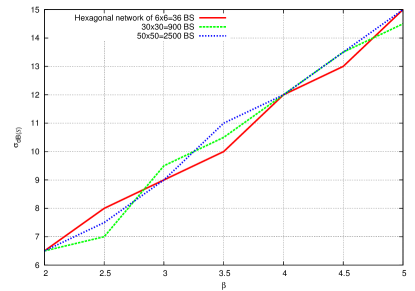
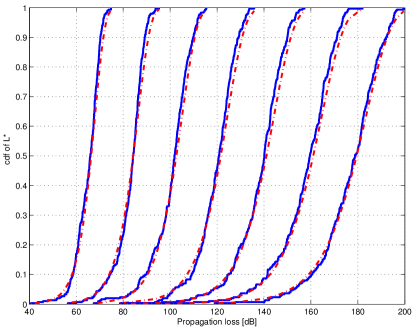
Figure 1: Critical values of $\sigma_{\mathrm{dB}}$ in function of the path-loss exponent $\beta$, for different network sizes, above which, the empirical distribution of $L^{\ast}$ in the hexagonal network cannot be distinguished from this for the “equivalent” Poisson model at a 99% confidence level, for 9/10 realizations of the hexagonal network.

Figure 2: Visual comparison of the empirical distribution of $L^{\ast}$ in the hexagonal network of $6\times 6=36$ base stations (solid lines) to the theoretical cdf of $L^{\ast}$ in the “equivalent” Poisson model (dashed lines) for $\beta=2,2.5,3,\ldots,5$ (curves from left to right) and the corresponding critical values of $\sigma_{\mathrm{dB}}=\sigma_{\mathrm{dB}}(\beta)$ taken from Figure 2.

Signal to interference (SIR) distribution

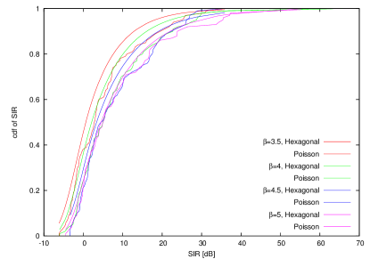
Figure 3: Empirical CDF of SIR simulated in hexagonal network with shadowing and their Poisson approximations.

Consider again Poisson and a hexagonal network consisting of $30\times 30=900$ base stations on a torus, with log-normal shadowing with the same parameters. For these two networks we compare the distribution of the SIR with respect to the strongest station

$$\text{SIR}=\frac{L^{*}}{\sum_{L_{i}\in\Theta}{L_{i}}-L^{*}}\,.$$

Recall that the analytic expression distribution of the SIR in Poisson network is known; cf [29, 42]. In Figure 3 we present a few examples of these CDF’s. We found that for $9/10$ realizations of the network shadowing the K-S test does not allow one to distinguish the empirical (obtained from simulations) CDF of the SIR from the CDF of SIR evaluated in the infinite Poisson model with the critical $p$-value fixed to $\alpha=10\%$ provided $\sigma_{\mathrm{dB}}$ is large enough.

V-B Linear-regression estimation of parameters

Based on the Poisson model, we will now suggest a method for the estimation of path-loss exponent $\beta$ from the measurements of the weakest propagation loss $L^{\ast}$ (performed by users in operational networks and known by the network operator). Corollary 14 implies that

$$\log\left(-\log\left[\mathbf{P}\left(L^{\ast}\geq t\right)\right]\right)=\log a+\frac{2}{\beta}\log t$$ (32)

Consequently, if the distribution of $L^{\ast}$ is available from measurements (or simulations), then one can estimate $\beta$ and $a$ by the linear regression between $\log\left(-\log\left[\mathbf{P}\left(L^{\ast}\geq t\right)\right]\right)$ and $\log t$. This characterizes in particular the path-loss exponent $\beta$.

We will now apply this method with respect to data obtained from simulations and from measurements of $L^{\ast}$ realized and collected in the cellular network of Orange in a certain large city in Europe, with density $\lambda=5.09\text{km}^{-2}$. For this dense urban area, we shall deduce the outdoor and then the indoor path-loss exponent $\beta$.

V-B1 Outdoor

The base stations positions are those of the UMTS network of Orange in a certain large city in Europe, operating with the carrier frequency of $2.1$GHz. The distribution of the outdoor propagation loss $L^{\ast}$ with the serving base station is obtained by simulations performed with StarWave, a propagation software developed by Orange Labs . The linear fitting (32) of the empirical data obtained from these simulations gives $\beta=3.85$;. This result can be validated by comparing it to the value of $\beta$ given for example by the COST Walfisch-Ikegami propagation model [38]. Indeed, considering the COST Walfisch-Ikegami model for the same frequency $2.1$GHz one obtains $\beta=3.80$ for the non-line-of-sight propagation loss. Observe that the values of $\beta$ obtained by the two different approaches are close to each other, which may validate the novel approach for the data under consideration.

V-B2 Indoor

We now consider the actual users’ data collected in the GSM network of Orange operating with a $1.8$GHz carrier frequency . The operator estimates that approximately $80\%$ of users are indoors and the remaining $20\%$ outdoors. The linear fitting (32) gives $\beta=3.64$;. We are not aware of any alternative model valid for indoor scenario; the COST Walfisch-Ikegami model being only valid for outdoor scenario.

VI Conclusion

We presented a convergence result to show that in the presence of sufficiently large log-normal-based shadowing the propagation processes (and, hence, SINR, spectral efficiency, etc,) experienced by a typical user in an empirically homogeneous wireless network behave stochastically as though the underlying base station configurations were scattered according to a homogeneous Poisson point process. In this shadowing regime, we also show that the distances to each base station are independent log-normal variables, hence the propagation process has become decoupled from the underlying geometry. This decoupling carries a trade-off between exact geometric information being lost and a considerable increase in tractability. Based on these findings, we presented a linear-regression method for estimating the exponent of the path-loss function based on user data in an empirically homogeneous cellular network with sufficiently large log-normal shadowing. This novel method for estimating statistical parameters of the propagation model complements other models such as those of Hata or COST Walfisch-Ikegami.

-A Proof of Proposition 3

By the displacement theorem [43, Section 1.3.3] $\tilde{\Theta}$ is an independently marked Poisson point process with intensity measure

$$\tilde{\Lambda}((0,y)\times(0,\rho)\times\tau) =2\pi\lambda\mathbf{E}\int_{0}^{\infty}\mathbf{1}((rK)^{\beta}/S\leq y)\mathbf{1}(r\leq\rho)\mathbf{1}(T\in\tau)r\,dr$$

$$=\pi\lambda\mathbf{E}[\min(\rho^{2},(yS)^{2/\beta}/K^{2}))\mathbf{1}(T\in\tau)]$$

$$=\frac{\pi\lambda}{K^{2}}\mathbf{E}[S^{2/\beta}\min((\rho K)^{2}/S^{2/\beta},y^{2/\beta})\mathbf{1}(T\in\tau)]$$

$$=\frac{\pi\lambda}{K^{2}}\mathbf{E}[S^{2/\beta}\min((\ell(\rho)/S)^{2/\beta},y^{2/\beta})\mathbf{1}(T\in\tau)]$$

$$=\frac{2\pi\lambda}{\beta K^{2}}\mathbf{E}[S^{2/\beta}\int_{0}^{y}\mathbf{1}(S\leq\ell(\rho)/u)\mathbf{1}(T\in\tau)u^{2/\beta-1}\,du]$$

$$=\frac{2\pi\lambda\mathbf{E}(S^{2/\beta})}{\beta K^{2}\mathbf{E}(S^{2/\beta})}\int_{0}^{y}\mathbf{E}[S^{2/\beta}\mathbf{1}(S\leq\ell(\rho)/u)\mathbf{1}(T\in\tau)]u^{2/\beta-1}\,du\,,$$

where in the last line we exchanged the integral and expectation. Putting $\rho=\infty$ and $\tau=\mathcal{T}$ allows one to recognize that

$$\Lambda(du) =\frac{2\pi\lambda\mathbf{E}(S^{2/\beta})}{\beta K^{2}}u^{2/\beta-1}du$$

$$=a\frac{2}{\beta}u^{2/\beta-1}du,$$

is the intensity measure of the unmarked process $\Theta$.

-B Proof of Proposition 5

Write $h_{\rho}:=(K\rho)^{\beta}/u$ and observe that

$$\mathbf{E}\Bigl{[}S^{2/\beta}\mathbf{1}(S\leq h_{\rho})\mathbf{1}(T\in\tau)]) =\mathbf{E}[S^{2/\beta}\mathbf{1}(S\leq h_{\rho})G^{T|S}(\tau|S)\Bigr{]}$$

$$=\frac{1}{\sqrt{2\pi}}\!\!\int_{-\infty}^{\infty}e^{-\frac{t^{2}}{2}+\frac{2\sigma t+2\mu}{\beta}}\mathbf{1}(e^{\sigma t+\mu}\leq h_{\rho})G^{T|S}(\tau|e^{\sigma t+\mu})dt.$$

Some algebra and (13) gives

$$\mathbf{E}[S^{2/\beta}\mathbf{1}(S\leq h_{\rho})\mathbf{1}(T\in\tau)]/\mathbf{E}(S^{2/\beta}) =\frac{1}{\sqrt{2\pi}}\int_{-\infty}^{\infty}e^{-\frac{(t-2\sigma/\beta)^{2}}{2}}\mathbf{1}(e^{\sigma t+\mu}\leq h_{\rho})G^{T|S}(\tau|e^{\sigma t+\mu})dt$$

$$=\frac{1}{\sqrt{2\pi}}\int_{-\infty}^{\infty}e^{-\frac{t^{2}}{2}}\mathbf{1}(e^{\sigma t+\mu+\frac{2\sigma^{2}}{\beta}}\leq h_{\rho})G^{T|S}(\tau|e^{\sigma t+\mu+\frac{2\sigma^{2}}{\beta}})dt$$

$$=\mathbf{E}\Bigl{[}\mathbf{1}(Se^{2\sigma^{2}/\beta}\leq(K\rho)^{\beta}/u)G^{T|S}(\tau|Se^{2\sigma^{2}/\beta})\Bigr{]}\,.$$

Equations (15) and (16) follow from (14) by assuming $\rho=\infty$ and $\tau=\mathcal{T}$, respectively.

-C Proof of Theorem 7

We simplify (and slightly abuse) the notation by setting $n:=\sigma^{2}$ and write $n$ instead of $n^{1/2}$ in the subscripts and superscripts. Let $n$ takes positive integer values without loss of generality. Furthermore, it is more convenient to study the propagation loss process $\widetilde{\Theta}$ on the logarithmic scale, hence we denote by $\Lambda_{\log}$ the image of the measure $\Lambda$ given in Lemma 1 through the logarithmic mapping; i.e.,

$$\Lambda_{\log}((-\infty,s]):=\int_{R^{+}}\mathbf{1}(\log(t)\leq s)\,\Lambda(dt)=\frac{\lambda\pi}{K^{2}}\exp\left[\frac{2s}{\beta}\right]$$ (33)

for $s\in\mathbb{R}$.

For all $n\geq 1$ and $r\geq 0$ we define and observe by (12) and (19) that

$$\nu_{n}(s,r) :=\mathbf{P}\left[\log\left(\frac{(K^{(n)})^{\beta}r^{\beta}}{S^{(n)}}\right)\leq s\right]$$

$$=\mathbf{P}\left[Z\geq-\frac{s-\beta\log(Kr)-n/\beta}{\sqrt{n}}\right]$$

$$=G_{Z}\left[\frac{s-\beta\log(Kr)-n/\beta}{\sqrt{n}}\right],$$ (34)

where $G_{Z}$ is the CDF of the standard Gaussian random variable.

Let $B_{0}(r)=\{x\in\mathbb{R}^{2}:|x|<r\}$. We now need to derive two results.

Lemma 15

$$\lim_{n\rightarrow\infty}\int_{B_{0}(b_{n})\setminus B_{0}(a_{n})}\nu_{n}(s,|x|)\,\lambda dx =\lim_{n\rightarrow\infty}\int_{\mathbb{R}^{2}}\nu_{n}(s,|x|)\,\lambda dx$$

$$=\Lambda_{\log}((-\infty,s])$$

provided that $a_{n}$ and $b_{n}$ satisfy (21) and (22).

Proof:

We first examine the integral over $B_{0}(b_{n})\setminus B_{0}(a_{n})$ in polar coordinates

$$\int_{B_{0}(b_{n})\setminus B_{0}(a_{n})}\nu_{n}(s,|x|)dx=2\pi\int_{a_{n}}^{b_{n}}rG_{Z}\left(\frac{s-\beta\log(Kr)-n/\beta}{\sqrt{n}}\right)dr.$$ (35)

The change of variables $t=(s-\beta\log(Kr)-n/\beta)/\sqrt{n}$ gives

$$2\pi\int_{a_{n}}^{b_{n}}rG_{Z}\left(\frac{s-\beta\log(Kr)-n/\beta}{\sqrt{n}}\right)dr$$

$$=2\pi\int_{v_{n}}^{u_{n}}\frac{1}{K^{2}}\exp\left[\frac{2}{\beta}\left(s-t\sqrt{n}-n/\beta\right)\right]G_{Z}(t)\frac{\sqrt{n}}{\beta}dt$$

$$=2\pi\frac{\sqrt{n}}{\beta}\frac{\exp\left[\frac{2}{\beta}\left(s-\frac{n}{\beta}\right)\right]}{K^{2}}\int_{-u_{n}}^{-v_{n}}\exp\left[\frac{2t\sqrt{n}}{\beta}\right]{G_{Z}}(-t)\,dt$$ (36)

where

$$u_{n}=\frac{s-\beta\log(Ka_{n})-n/\beta}{\sqrt{n}},$$ (37)

$$v_{n}=\frac{s-\beta\log(Kb_{n})-n/\beta}{\sqrt{n}}\,.$$ (38)

Moreover,

$$\int_{-u_{n}}^{-v_{n}}\exp\left[\frac{2t\sqrt{n}}{\beta}\right]{G_{Z}}(-t)dt= \left.\frac{\beta}{2\sqrt{n}}\exp\left[\frac{2t\sqrt{n}}{\beta}\right]{G_{Z}}(-t)\right|_{t=-u_{n}}^{t=-v_{n}}$$ (39)

$$+\frac{\beta}{2\sqrt{n}}\exp\left[\frac{2n}{\beta^{2}}\right]\int_{-u_{n}}^{-v_{n}}\exp\left[-\frac{1}{2}\left(t-\frac{2\sqrt{n}}{\beta}\right)^{2}\right]\frac{dt}{\sqrt{2\pi}}.$$ (40)

Combining (35), (36) and (39)–(40) we have

$$\int_{B_{0}(b_{n})\setminus B_{0}(a_{n})}\nu_{n}(s,|x|)dx= \left.\frac{\pi}{K^{2}}\exp\left[\frac{2}{\beta}\left(s-\frac{n}{\beta}+t\sqrt{n}\right)\right]{G_{Z}}(-t)\right|_{-u_{n}}^{-v_{n}}$$ (41)

$$+\frac{\pi}{K^{2}}\exp\left[\frac{2s}{\beta}\right]\int_{-u_{n}-\frac{2\sqrt{n}}{\beta}}^{-v_{n}-\frac{2\sqrt{n}}{\beta}}e^{-\frac{w^{2}}{2}}\frac{dw}{\sqrt{2\pi}},$$ (42)

where in the last integral we have changed the variable $w=t-2\sqrt{n}/\beta$. Note first that the integrated term (41) is finite even if $v_{n}=-\infty$ (which is equivalent to $b_{n}=\infty$) for some $n$, which can be deduced from the inequality

$$G_{Z}(-t)=1-G_{Z}(t) =\frac{1}{\sqrt{2\pi}}\int_{t}^{\infty}e^{-x^{2}/2}dx\leq e^{-t^{2}/2},\quad t\geq 0\,,$$ (43)

(see [44, Section 7.8]). By (37)–(38)

$$-u_{n} =\sqrt{n}\left(\frac{\beta\log(a_{n})}{n}+\frac{1}{\beta}\right)+o(1)$$ (44)

$$-v_{n} =\sqrt{n}\left(\frac{\beta\log(b_{n})}{n}+\frac{1}{\beta}\right)+o(1)$$ (45)

as $n\to\infty$. Consequently, under conditions (21) and (22) respectively, $-u_{n}-2\sqrt{n}/\beta\to-\infty$ and $-v_{n}-2\sqrt{n}/\beta\to\infty$, making the term (42) converge to $\lambda^{-1}\Lambda_{\log}((-\infty,s])$.

Regarding the integrated term (41), by (22) and (45), $\log(b_{n})/n\to\infty$ and $v_{n}\to-\infty$ by (43)

$$\exp\left[\frac{2}{\beta}\left(s-\frac{n}{\beta}-v_{n}\sqrt{n}\right)\right]{G_{Z}}(v_{n}) \leq\exp\left[\frac{2}{\beta}\left(s-\frac{n}{\beta}\right)+\frac{v_{n}}{2}\left(-v_{n}-\frac{4\sqrt{n}}{\beta}\right)\right]$$

$$=\exp\left[\frac{2}{\beta}\left(s-\frac{n}{\beta}\right)+\frac{\sqrt{n}v_{n}}{2}\left(\frac{\beta\log(b_{n})}{n}-\frac{3}{\beta}+o(\frac{1}{\sqrt{n}})\right)\right]$$

$$\to 0\qquad(n\to\infty).$$

Considering the term containing $-u_{n}$ in (41), it is easy to see that it converges to 0 when $-u_{n}\leq 0$ (by the trivial bound $G_{Z}(-t)\leq 1$). We will thus consider from now only $-u_{n}\geq 0$. Moreover by  (21) and (37) we have also $-u_{n}\leq\sqrt{n}\Bigl{(}1/\beta+o(1)\Bigr{)}$. For such values $-u_{n}$ we use again (43) and observing that the function $-2u_{n}\sqrt{n}/\beta-{u^{2}_{n}}/{2}={u_{n}}/{2}\left(-u_{n}-{4\sqrt{n}}/{\beta}\right)$ is increasing in $-u_{n}$ for $-u_{n}\leq 2\sqrt{n}/\beta$ we obtain

$$\exp\left[\frac{2}{\beta}\left(s-\frac{n}{\beta}-u_{n}\sqrt{n}\right)\right]{G_{Z}}(u_{n}) \leq\exp\left[\frac{2}{\beta}\left(s-\frac{n}{\beta}-u_{n}\sqrt{n}\right)-\frac{u^{2}_{n}}{2}\right]$$

$$\leq\exp\left[\frac{2}{\beta}\left(s-\frac{n}{\beta}\right)+\frac{u_{n}}{2}\left(-u_{n}-\frac{4\sqrt{n}}{\beta}\right)\right]$$

$$\leq\exp\left[\frac{2}{\beta}\left(s-\frac{n}{\beta}+n\Bigl{(}\frac{1}{\beta}+o(1)\Bigr{)}\right)-\frac{n}{2}\Bigl{(}\frac{1}{\beta}+o(1)\Bigr{)}^{2}\right]$$

$$=\exp\left[\frac{2}{\beta}\left(s-n\Bigl{(}\frac{1}{4\beta}+o(1)\Bigr{)}\right)\right]\to 0\quad(n\to\infty),$$

which concludes the proof of Lemma 15. ∎

Lemma 16

Assume (18), (21) and (22), then

$$\lim_{n\rightarrow\infty}\sum_{X_{i}\in\phi\cap(B_{0}(b_{n})\setminus B_{0}(a_{n}))}\nu_{n}(s,|X_{i}|) =\lim_{n\rightarrow\infty}\sum_{X_{i}\in\phi}\nu_{n}(s,|X_{i}|)=\Lambda_{\log}((-\infty,s]).$$ (46)

Proof:

For $k\geq 0$ and a fixed $\epsilon>0$, let $r_{k}=e^{\epsilon k}$ and $A_{k}=B_{0}(r_{k+1})\setminus B_{0}(r_{k})$, and write the summation in (46) as

$$\sum_{X_{i}\in\phi}\nu_{n}(s,|X_{i}|) =\sum_{X_{i}\in\phi\cap B_{0}(r_{k_{0}})}\nu_{n}(s,|X_{i}|)+\sum_{k=k_{0}}^{\infty}\sum_{X_{i}\in\phi\cap A_{k}}\nu_{n}(s,|X_{i}|),$$ (47)

for some $k_{0}\geq 0$, whose value will be fixed later on. In the limit when $n\rightarrow\infty$, the first summation in (47) vanishes; indeed

$$\sum_{X_{i}\in\phi\cap B_{0}(r_{k_{0}})}\nu_{n}(s,|X_{i}|) =\sum_{X_{i}\in\phi\cap B_{0}(r_{k_{0}})}\mathbf{P}\left[Z\leq\frac{s-\beta\log(K|X_{i}|)-n/\beta}{\sqrt{n}}\right]$$

$$=\sum_{X_{i}\in\phi\cap B_{0}(r_{k_{0}})}G_{Z}\left(\frac{s-\beta\log(K|X_{i}|)-n/\beta}{\sqrt{n}}\right)$$

$$\leq\phi(B_{0}(r_{k_{0}}))G_{Z}\left(\frac{s-\beta\log(K|X_{*}|)-n/\beta}{\sqrt{n}}\right)\rightarrow 0\quad(n\rightarrow\infty),$$

where $X_{*}$ gives the maximum of $G_{Z}\left(\frac{s-\beta\log(K|X|)-n/\beta}{\sqrt{n}}\right)$ over $X\in\phi\cap B_{0}(r_{k_{0}})$ which exists since $\phi$ is (by our assumption) a locally finite point measure. For the second summation in (47) we write $\nu_{n}(s,|X_{i}|)=\nu_{n}(s,|x|\frac{|X_{i}|}{|x|})$, hence

$$\nu_{n}(s,|X_{i}|)=\frac{1}{|A_{k}|}\int_{A_{k}}\nu_{n}\left(s,|x|\frac{|X_{i}|}{|x|}\right)dx.$$

Then the bounds for $x,X_{i}\in A_{k}$

$$e^{-\epsilon}=\frac{r_{k}}{r_{k+1}}\leq\frac{|X_{i}|}{|x|}\leq\frac{r_{k+1}}{r_{k}}=e^{\epsilon},$$

and the expression (34) of $\nu_{n}$, which implies $\nu_{n}(s,|x|e^{\epsilon})=\nu_{n}(s-\beta\epsilon,|x|)$, lead to the lower bound

$$\sum_{k=k_{0}}^{\infty}\sum_{X_{i}\in\phi\cap A_{k}}\nu_{n}(s,|X_{i}|)\geq\sum_{k=k_{0}}^{\infty}\frac{\phi(A_{k})}{|A_{k}|}\int_{A_{k}}\nu_{n}(s-\beta\epsilon,|x|)dx,$$ (48)

and the upper bound

$$\sum_{k=k_{0}}^{\infty}\sum_{X_{i}\in\phi\cap A_{k}}\nu_{n}(s,|X_{i}|)\\ \leq\sum_{k=k_{0}}^{\infty}\frac{\phi(A_{k})}{|A_{k}|}\int_{A_{k}}\nu_{n}(s+\beta\epsilon,|x|)dx.$$ (49)

Moreover, we write

$$\frac{\phi(A_{k})}{|A_{k}|} =\frac{\phi(B_{0}(r_{k+1}))-\phi(B_{0}(r_{k}))}{|B_{0}(r_{k+1})|-|B_{0}(r_{k})|}$$

$$=\frac{\frac{\phi(B_{0}(r_{k+1}))}{|B_{0}(r_{k+1})|}-\frac{\phi(B_{0}(r_{k}))}{|B_{0}(r_{k})|}\frac{|B_{0}(r_{k})|}{|B_{0}(r_{k+1})|}}{1-\frac{|B_{0}(r_{k})|}{|B_{0}(r_{k+1})|}}$$

$$=\frac{\frac{\phi(B_{0}(r_{k+1}))}{|B_{0}(r_{k+1})|}-\frac{\phi(B_{0}(r_{k}))}{|B_{0}(r_{k})|}e^{-2\epsilon}}{1-e^{-2\epsilon}},$$

and the requirement (18) yields $\lim_{k\rightarrow\infty}\frac{\phi(A_{k})}{|A_{k}|}=\lambda$. Hence, for any fixed $\delta>0$, there exists a $k_{0}(\delta)$ such that for all $k\geq k_{0}$, the bounds

$$(1-\delta)\lambda\leq\frac{\phi(A_{k})}{|A_{k}|}\leq(1+\delta)\lambda,$$

hold. Lower bound (48) becomes

$$\sum_{k=k_{0}}^{\infty}\sum_{X_{i}\in\phi\cap A_{k}}\!\!\!\nu_{n}(s,|X_{i}|) \geq\sum_{k=k_{0}}^{\infty}(1-\delta)\lambda\int_{A_{k}}\!\!\!\nu_{n}(s-\beta\epsilon,|x|)dx,$$

$$=(1-\delta)\lambda\int_{|x|\geq r_{k_{0}}}\!\!\!\!\!\nu_{n}(s-\beta\epsilon,|x|)dx\,.$$

Finally, Lemma 15 allows us to set $a_{n}=r_{k_{0}}$ and $b_{n}=\infty$, hence

$$\lim_{n\rightarrow\infty}\sum_{k=k_{0}}^{\infty}\sum_{X_{i}\in\phi\cap A_{k}}\nu_{n}(s,|X_{i}|)\geq(1-\delta)\frac{\pi\lambda}{K^{2}}\exp\left[\frac{2(s-\beta\epsilon)}{\beta}\right],$$

and similarly the upper bound (49) becomes

$$\lim_{n\rightarrow\infty}\sum_{k=k_{0}}^{\infty}\sum_{X_{i}\in\phi\cap A_{k}}\nu_{n}(s,|X_{i}|)\leq(1+\delta)\frac{\pi\lambda}{K^{2}}\exp\left[\frac{2(s+\beta\epsilon)}{\beta}\right]\,.$$

Letting $\epsilon\rightarrow 0$ and $\delta\rightarrow 0$ completes the proof of (46). The other result, (46), can be proved by a straightforward modification of the above arguments. ∎

Proof:

The classical convergence result [11, Theorem 11.2.V] in conjunction with [11, (11.4.2) and (11.4.3)] says that the propagation loss process $\widetilde{\Theta}$ converges to the Poisson limit provided

$$\sup_{i}\nu^{i}_{n}(A)\rightarrow 0\quad(n\rightarrow\infty).$$ (50)

and

$$\sum_{i}\nu^{i}_{n}(A)\rightarrow\Lambda_{\log}(A)\quad(n\rightarrow\infty),$$ (51)

for all bounded Borel sets $A\subset\mathbb{R}$, where $\nu_{n}^{i}(\cdot)$ is the (probability) measure on $\mathbb{R}$ defined by setting $\nu_{n}^{i}((-\infty,s]):=\nu_{n}(s,|X_{i}|)$. The first condition, (50), clearly holds by (34) for any locally finite $\phi$ without a point at the origin. The second condition, (51) follows from Lemma 16, which establish the required convergence for $A=(-\infty,s]$ and any $s\in\mathbb{R}$. This is enough to conclude the convergence for all bounded Borel sets. ∎

-D Proof of Theorem 10

We begin by explaining the pertinence of our assumptions (23) and (24). Let $S^{(\sigma)}$ be given by (12), with $\mu=-\sigma^{2}/2$, and denote by $G^{T|Z}(\tau|z)$, $z\in\mathbb{R}$, $\tau\in\mathcal{T}$, the conditional distribution of the mark $T$ given $Z$ (which is, recall, a standard Gaussian random variable)

$$G^{T^{(\sigma)}|Z}(\tau|z):=G^{T^{(\sigma)}|S^{(\sigma)}}(\tau|e^{-\sigma^{2}/2+\sigma z})\,.$$ (52)

Then a simple algebra allows one to express $G_{u}(\rho,\tau)$ given by (14), with $K^{(\sigma)}$ given by (19) and $S^{(\sigma)}$ as above in the following way

$$G_{u}(\rho,\tau)=\mathbf{E}\left[\mathbf{1}\left(Z\leq\frac{\beta\log\rho}{\sigma}-\frac{\sigma}{\beta}-\frac{\beta\log k-\log u}{\sigma}\right)G^{T^{(\sigma)}|Z}\left(\tau\Big{|}Z+\frac{2\sigma}{\beta}\right)\right]\,.$$ (53)

Note that $(\beta\log k-\log u)/\sigma$ vanishes when $\sigma\to\infty$ making the conditional distribution $G_{u}(\rho,\tau)$ (of the distance and type of the base station whose propagation loss is equal to $u$) independent of $u$. Furthermore, (53) suggests (23) as the scaling of the distance to the base station and (24) for the conditional distribution of the type $T_{i}^{(\sigma)}$ of the base station given the shadowing $S^{(\sigma)}$.

We proceed now to the proof of Theorem 10. In analogy to (33) we define the image of the measure $\tilde{\Lambda}$ given in Theorem 10 through the logarithmic mapping of the propagation loss values

$$\tilde{\Lambda}_{\log}((-\infty,s]\times(-\infty,\rho]\times\tau)=\frac{\lambda\pi}{K^{2}}\exp\left[\frac{2s}{\beta}\right]G(\rho;\tau)$$

for $s\in\mathbb{R}$, $\rho\in\mathbb{R}$ and $\tau\in\mathcal{T}$. Similarly, we extend the measures (34) for $n\geq 1$, $r,\rho\geq 0$ and $\tau\in\mathcal{T}$ and observe that, by (23) and (24)

$$\tilde{\nu}_{n}(s,\rho,\tau,r) :=\mathbf{P}\left[\log\left(\frac{(K^{(n)})^{\beta}r^{\beta}}{\exp[-n/2+\sqrt{n}Z]}\right)\leq s,\mathcal{R}(r)\leq\rho,T^{(n)}\in\tau\right]$$

$$=\mathbf{P}\left(Z\geq-\frac{s-\beta\log(Kr)-n/\beta}{\sqrt{n}},T^{(n)}\in\tau\right)\mathbf{1}(\mathcal{R}(r)\leq\rho)$$ (54)

$$=G^{*}\left(-\frac{s-\beta\log(Kr)-n/\beta}{\sqrt{n}};\tau\right)\mathbf{1}(\mathcal{R}(r)\leq\rho)\,,$$ (55)

where

$$G^{*}(z;\tau)=\int_{z}^{\infty}G^{T|Z}(\tau|z-2\sqrt{n}/\beta)\,G_{Z}(dz)\,.$$

With this notation we extend Lemma 15 (cf its proof for the details and $u_{n}$, $v_{n}$)

$$\int_{B_{0}(b_{n})\setminus B_{0}(a_{n})}\tilde{\nu}_{n}(s,\rho,\tau,|x|)dx =2\pi\!\!\int_{a_{n}}^{b_{n}}rG^{*}\left(-\frac{s-\beta\log(Kr)-n/\beta}{\sqrt{n}};\tau\right)\!\!\mathbf{1}\!\!\left(r\leq e^{\frac{\sqrt{n}}{\beta}(\rho+\frac{\sqrt{n}}{\beta})}\right)dr$$

$$=2\pi\frac{\sqrt{n}}{\beta}\frac{e^{\frac{2}{\beta}\left(s-n/\beta\right)}}{K^{2}}\int_{-u_{n}}^{-v_{n}}e^{\frac{2t\sqrt{n}}{\beta}}{\scriptstyle{G^{*}}(t;\tau)\mathbf{1}\left(t\leq\rho+\frac{2\sqrt{n}}{\beta}-\frac{s-\beta\log K}{\sqrt{n}}\right)}dt$$

$$=\left.\frac{\pi}{K^{2}}e^{\frac{2}{\beta}\left(s-\frac{n}{\beta}+t\sqrt{n}\right)}{G^{*}}(t;\tau){\scriptstyle\mathbf{1}\left(t\leq\rho+\frac{2\sqrt{n}}{\beta}-\frac{s-\beta\log K}{\sqrt{n}}\right)}\right|_{-u_{n}}^{-v_{n}}$$ (56)

$$\hskip 10.00002pt+\frac{\pi}{K^{2}}e^{\frac{2s}{\beta}}\int_{-u_{n}-\frac{2\sqrt{n}}{\beta}}^{-v_{n}-\frac{2\sqrt{n}}{\beta}}e^{-\frac{w^{2}}{2}}{\scriptstyle\mathbf{1}\left(w\leq\rho-\frac{s-\beta\log K}{\sqrt{n}}\right)}G^{T|Z}(\tau|w)\frac{dw}{\sqrt{2\pi}}$$

$$\hskip 80.00012pt\to\frac{\pi}{K^{2}}e^{\frac{2s}{\beta}}G(\rho;\tau)\qquad(n\to\infty),$$

because $0\leq G^{*}(t;\tau)\leq 1-G_{Z}(t)=G_{Z}(-t)$ thus the term (56), being dominated by (41), converges to 0. Moreover, using the same arguments as in the proof Lemma 16, with $\tilde{\nu}_{n}(s,\rho,\tau,re^{\epsilon})=\tilde{\nu}_{n}(s-\beta\epsilon,\rho-\beta\epsilon/\sqrt{n},\tau,r)$, one proves

$$\lim_{n\rightarrow\infty}\sum_{X_{i}\in\phi\cap(B_{0}(b_{n})\setminus B_{0}(a_{n}))}\tilde{\nu}_{n}(s,\rho,\tau,|X_{i}|)$$

$$=\lim_{n\rightarrow\infty}\sum_{X_{i}\in\phi}\tilde{\nu}_{n}(s,\rho,\tau,|X_{i}|)=\frac{\lambda\pi}{K^{2}}e^{\frac{2s}{\beta}}G(\rho;\tau)\,.$$

Now, the result follows by the same arguments as used in the proof of Theorem 7.

References

- [1] B. Błaszczyszyn and M. K. Karray, “Linear-regression estimation of the propagation-loss parameters using mobiles’ measurements in wireless cellular networ,” in Proc. of WiOpt, Paderborn, 2012.
- [2] B. Błaszczyszyn, M. K. Karray, and H. P. Keeler, “Using Poisson processes to model lattice cellular networks,” in Proc. of IEEE INFOCOM, 2013.
- [3] C.-H. Lee, C.-Y. Shih, and Y.-S. Chen, “Stochastic geometry based models for modeling cellular networks in urban areas,” Wireless networks, vol. 19, no. 6, pp. 1063–1072, 2013.
- [4] A. Guo and M. Haenggi, “Spatial stochastic models and metrics for the structure of base stations in cellular networks,” IEEE Trans. Wireless Comm., vol. 12, no. 11, 2013.
- [5] B. Błaszczyszyn, M. Jovanović, and M. K. Karray, “How user throughput depends on the traffic demand in large cellular networks,” in Proc. of WiOpt/SpaSWiN, 2014.
- [6] H. Dhillon, R. Ganti, F. Baccelli, and J. Andrews, “Modeling and analysis of K-tier downlink heterogeneous cellular networks,” IEEE J. Sel. Areas Commun., vol. 30, no. 3, pp. 550–560, april 2012.
- [7] H. Suzuki, “A statistical model for urban radio propogation,” Communications, IEEE Transactions on, vol. 25, no. 7, pp. 673–680, 1977.
- [8] C. S. Withers and S. Nadarajah, “A generalized Suzuki distribution,” Wireless Personal Communications, vol. 62, no. 4, pp. 807–830, 2012.
- [9] J. Reig and L. Rubio, “Estimation of the composite fast fading and shadowing distribution using the log-moments in wireless communications,” IEEE Trans. Wireless Comm., vol. 12, no. 8, pp. 3672–3681, 2013.
- [10] T. X. Brown, “Cellular performance bounds via shotgun cellular systems,” IEEE JSAC, vol. 18, no. 11, pp. 2443–2455, 2000.
- [11] D. J. Daley and D. Vere-Jones, An introduction to the theory of point processes. Vol. II. New York: Springer, 2008.
- [12] M. Haenggi, “A geometric interpretation of fading in wireless networks: Theory and applications,” IEEE Trans. Inf. Theory, vol. 54, no. 12, pp. 5500–5510, 2008.
- [13] B. Błaszczyszyn and H. P. Keeler, “Equivalence and comparison of heterogeneous cellular networks,” in Proc. of PIMRC Workshops, Sept 2013, pp. 153–157.
- [14] D. Ruelle, “A mathematical reformulation of Derrida’s REM and GREM,” Communications in Mathematical Physics, vol. 108, no. 2, pp. 225–239, 1987.
- [15] D. Panchenko and M. Talagrand, “Guerra’s interpolation using Derrida-Ruelle cascades,” arXiv preprint arXiv:0708.3641, 2007.
- [16] P. Madhusudhanan, J. G. Restrepo, Y. Liu, and T. X. Brown, “Carrier to interference ratio analysis for the shotgun cellular system,” in Proc. of IEEE GLOBECOM, 2009, pp. 1–6.
- [17] B. Błaszczyszyn, M. K. Karray, and F.-X. Klepper, “Impact of the geometry, path-loss exponent and random shadowing on the mean interference factor in wireless cellular networks,” in Proc. of IFIP WMNC, Budapest, Hungary, 2010.
- [18] T.-T. Vu, L. Decreusefond, and P. Martins, “An analytical model for evaluating outage and handover probability of cellular wireless networks,” Wireless Personal Communications, vol. 74, no. 4, pp. 1117–1127, 2014.
- [19] B. Błaszczyszyn and H. P. Keeler, “Studying the SINR process of the typical user in Poisson networks by using its factorial moment measures,” arXiv preprint arXiv:1401.4005, 2014, under review.
- [20] D. Panchenko, The Sherrington-Kirkpatrick model. Springer, 2013.
- [21] J. F. C. Kingman, Poisson Processes, 1st ed. Oxford University Press, 1993.
- [22] J. Pitman and M. Yor, “The two-parameter Poisson–Dirichlet distribution derived from a stable subordinator,” The Annals of Probability, vol. 25, no. 2, pp. 855–900, 1997.
- [23] H. P. Keeler and B. Błaszczyszyn, “SINR in cellular networks and the two-parameter Poisson-Dirichlet process,” IEEE Wireless Comm Letters, 2014, published on Early access on August 2014.
- [24] J. Andrews, F. Baccelli, and R. Ganti, “A tractable approach to coverage and rate in cellular networks,” IEEE Trans. Commun., vol. 59, no. 11, pp. 3122 –3134, november 2011.
- [25] P. Madhusudhanan, J. Restrepo, Y. Liu, and T. Brown, “Downlink coverage analysis in a heterogeneous cellular network,” in Proc. of IEEE GLOBECOM, 2012, pp. 4170–4175.
- [26] S. Mukherjee, “Distribution of downlink SINR in heterogeneous cellular networks,” IEEE JSAC, vol. 30, no. 3, pp. 575–585, 2012.
- [27] H. S. Dhillon, R. K. Ganti, and J. G. Andrews, “A tractable framework for coverage and outage in heterogeneous cellular networks,” in Proc. of IEEE ITA Workshop, 2011, pp. 1–6.
- [28] S. Mukherjee, Analytical Modeling of Heterogeneous Cellular Networks. Cambridge University Press, 2014.
- [29] H. P. Keeler, B. Błaszczyszyn, and M. K. Karray, “SINR-based k-coverage probability in cellular networks with arbitrary shadowing,” in Proc. of IEEE ISIT, 2013.
- [30] A. Giovanidis and F. Baccelli, “A stochastic geometry framework for analyzing pairwise-cooperative cellular networks,” arXiv preprint arXiv:1305.6254, 2013.
- [31] R. Tanbourgi, S. Singh, J. Andrews, and F. Jondral, “Analysis of non-coherent joint-transmission cooperation in heterogeneous cellular networks,” in Communications (ICC), 2014 IEEE International Conference on, June 2014, pp. 5160–5165.
- [32] X. Zhang and M. Haenggi, “Successive interference cancellation in downlink heterogeneous cellular networks,” in Proc. of IEEE GLOBECOM-HetSNets’13, Dec. 2013.
- [33] M. Wildemeersch, T. Q. Quek, M. Kountouris, A. Rabbachin, and C. H. Slump, “Successive interference cancellation in heterogeneous cellular networks,” arXiv preprint arXiv:1309.6788, 2013.
- [34] N. Miyoshi and T. Shirai, “A cellular network model with Ginibre configured base stations,” Advances in Applied Probability, vol. 46, no. 3, pp. 832–845, 2014.
- [35] I. Nakata and N. Miyoshi, “Spatial stochastic models for analysis of heterogeneous cellular networks with repulsively deployed base stations,” Performance Evaluation, 2014.
- [36] Y. Li, F. Baccelli, H. S. Dhillon, and J. G. Andrews, “Statistical modeling and probabilistic analysis of cellular networks with determinantal point processes,” arXiv preprint arXiv:1412.2087, 2014.
- [37] N. Deng, W. Zhou, and M. Haenggi, “The Ginibre point process as a model for wireless networks with repulsion,” Wireless Communications, IEEE Transactions on, vol. 14, no. 1, pp. 107–121, Jan 2015.
- [38] COST 231, Evolution of land mobile radio (including personal) communications, Final report, Information, Technologies and Sciences, European Commission, 1999.
- [39] W. C. Jakes, Microwave mobile communications. John Wiley and Sons, 1974.
- [40] H. P. Keeler, N. Ross, and A. Xia, “When do wireless network signals appear Poisson?” arXiv preprint arXiv:1411.3757, 2014.
- [41] D. Williams, Weighing The Odds: A Course In Probability And Statistics. Cambridge University Press, 2001.
- [42] H. P. Keeler, “SINR-based -coverage probability in cellular networks,” MATLAB Central File Exchange, 2013. [Online]. Available: http://www.mathworks.fr/matlabcentral/fileexchange/40087-sinr-based-k-coverage-probability-in-cellular-networks
- [43] F. Baccelli and B. Błaszczyszyn, Stochastic Geometry and Wireless Networks, Volume I — Theory, ser. Foundations and Trends in Networking. NoW Publishers, 2009, vol. 3, No 3–4.
- [44] (2012, Accessed on the 10th of September) Digital Library of Mathematical Functions. National Institute of Standards and Technology. Release 1.0.5 of 2012-10-01. [Online]. Available: http://dlmf.nist.gov/