EXCLUSIVE QUEUEING PROCESSES AND THEIR APPLICATION TO TRAFFIC SYSTEMS

Abstract

The dynamics of pedestrian crowds has been studied intensively in recent years, both theoretically and empirically. However, in many situations pedestrian crowds are rather static, e.g. due to jamming near bottlenecks or queueing at ticket counters or supermarket checkouts. Classically such queues are often described by the M/M/1 queue that neglects the internal structure (density profile) of the queue by focussing on the system length as the only dynamical variable. This is different in the Exclusive Queueing Process (EQP) in which the queue is considered on a microscopic level. It is equivalent to a Totally Asymmetric Exclusion Process (TASEP) of varying length. The EQP has a surprisingly rich phase diagram with respect to the arrival probability $\alpha$ and the service probability $\beta$. The behavior on the phase transition line is much more complex than for the TASEP with a fixed system length. It is nonuniversal and depends strongly on the update procedure used. In this article, we review the main properties of the EQP. We also mention extensions and applications of the EQP and some related models.

(xxxxxxxxxx)

AMS Subject Classification: 60K25, 90B20, 82C22

1 Introduction

Queueing processes have been studied extensively for decades [1, 2]. Although originally developed to describe problems of telecommunication, they have been applied later also to various kinds of jamming phenomena, e.g. supply chains and vehicular traffic (see Sec. 11). However, classical queueing theory neglects the spatial structure of queues and the customers (particles) in queues do not interact with each other. The length $L_{t}$ of the system is the only dynamical variable and the density along the queue is constant. Therefore an extension of the classical M/M/1 queueing process has been introduced recently [3, 4]. It takes into account particle interactions through the excluded-volume effect and leads to nontrivial density profiles of the queue.

Classical queueing theory has been introduced more than 100 years ago with the seminal works by Erlang [5]. It is closely related to the theory of Markov chains and has found many applications ranging from telecommunication and traffic flow to economics. Queueing models are usually classified according to the type of the arrival processes, the service time distribution and the number of queues, which are denoted by Kendall’s notation. The queue discipline (e.g. First-In-First-Out (FIFO) or Last-In-First-Out (LIFO)) is also an important classification.

2 Markov chains and classical queueing theory

Markov chains (or Markov processes) [6] have become an important tool to phenomenologically describe physical systems [7, 8, 9, 10, 11]. The dynamics of a Markov chain with discrete time $t$ on a state space $S$, which is a countable set, is governed by

$$P(\tau;t+1)=\sum_{\tau^{\prime}\in S}W(\tau^{\prime}\to\tau)P(\tau^{\prime};t),$$ (1)

where $W(\tau^{\prime}\to\tau)$ is the transition probability from $\tau^{\prime}$ to $\tau$ , and $P(\tau;t)\ (\tau\in S)$ is the probability of finding the state $\tau$ at time $t$. Physicists often call this equation “master equation” [8]. When we achieve any $\tau_{f}\in S$ from any $\tau_{i}\in S$ (i.e. there is a path $\tau_{i}\to\tau_{1}\to\cdots\tau_{n}\to\tau_{f}$ such that $W(\tau_{i}\to\tau_{1})W(\tau_{1}\to\tau_{2})\dots W(\tau_{n}\to\tau_{f})>0$), we say that the system is irreducible.

The (a)periodicity is also of importance for the Markov processes. The period of a state $\tau\in S$ is defined as gcd$\{n|W(\tau\to\tau_{1})\cdots W(\tau_{n}\to\tau)>0\}$ (greatest common divisor). For an irreducible Markov process, all the states have the same period. When the period is 1, we say the process is aperiodic. Note that if a process has at least one state $\tau$ such that $W(\tau\to\tau)>0$, the process is aperiodic.

The stationary measure is the solution to

$$P_{st}(\tau)=\sum_{\tau^{\prime}\in S}W(\tau^{\prime}\to\tau)F(\tau^{\prime}).$$ (2)

When a stationary measure $P_{st}(\tau)$ is normalizable, i.e. $\sum_{\tau\in S}P_{st}(\tau):=Z$ is finite, we can construct a stationary distribution by $\frac{1}{Z}P_{st}(\tau)$. For an irreducible and aperiodic system, a stationary distribution is unique, if it exists, and we have the important property $\lim_{t\to\infty}P(\tau;t)=\frac{1}{Z}P_{st}(\tau)$ [6] .

When a stationary distribution does not exist, we have $\lim_{t\to\infty}P(\tau;t)=0$ for all $\tau\in S$.

2.1 M/M/1 queue

The M/M/1 queueing process describes the dynamics of a single queue with one server where arrival and service processes are Poissonian. We usually treat it as a FIFO queue. It is defined by the arrival probability $\alpha$ and service probability $\beta$ [1, 2]. Customers ($=$ particles) arrive with probability $\alpha$ at the end of the queue and are serviced ($=$ removed) with probability $\beta$ at the front of the queue (Fig. 1). Assuming that the particles representing customers have unit length, the length $L_{t}$ of the queue at time $t$ is identical to the number of particles $N_{t}$. In other words, in the M/M/1 queueing process, the internal structure of the queue is not considered.

For the discrete time M/M/1 queue, the probability $P(L;t)$ of having the length $L$ at time $t$ is governed by the master equation

$$P(0;t+1)= (1-\alpha)P(0;t)+\alpha\beta P(0;t)+(1-\alpha)\beta P(1;t)$$ (3)

$$\begin{split}P(L;t+1)=&\alpha(1-\beta)P(L-1;t)+[(1-\alpha)(1-\beta)+\alpha\beta]P(L;t)\\ &+(1-\alpha)\beta P(L+1;t)\,.\end{split}$$ (4)

One can easily find a stationary measure

$$P_{st}(L)=\left(\frac{\alpha(1-\beta)}{(1-\alpha)\beta}\right)^{L}\,.$$ (5)

For $\alpha<\beta$, a unique stationary distribution exists, which is given by the geometric distribution

$$P(L)=\frac{\beta-\alpha}{(1-\alpha)\beta}\left(\frac{\alpha(1-\beta)}{(1-\alpha)\beta}\right)^{L}\,.$$ (6)

The average length is then given by $\langle L\rangle=\sum_{L\geq 1}LP(L)$. For $\alpha\geq\beta$, no stationary distribution exists and $\lim_{t\to\infty}P(L;t)=0$ for all given $L$. In other words, the queue diverges. Therefore the M/M/1 queue has two phases, according whether the queue length diverges or converges:

$$\lim_{t\to\infty}\langle L_{t}\rangle=\begin{cases}\infty&\qquad\text{for }\alpha\geq\beta,\\ \frac{\alpha(1-\beta)}{\beta-\alpha}&\qquad\text{for }\alpha<\beta.\end{cases}\,$$ (7)

The phases are separated by the critical line $\alpha=\beta$ (Fig. 1).

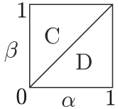
Figure 1: Definition of M/M/1 queue (left) and its phase diagram (right). When the arrival probability $\alpha$ is larger than service probability $\beta$, the queue Diverges (D). It Converges (C) when $\alpha<\beta$.

Let us consider the inflow $J_{\text{in}}$ and outflow $J_{\text{out}}$ of customers in the limit $t\to\infty$. By definition, we always have $J_{\text{in}}=\alpha$, whereas the outflow depends on the parameters. In the convergent phase, the flows must be balanced. In fact we find

$$J_{\text{out}}=\beta\sum_{L\geq 1}P(L)+\alpha\beta P(0)=\alpha.$$ (8)

On the other hand, in the divergent phase, the length becomes always larger than 0, and thus we have

$$J_{\text{out}}=\beta.$$ (9)

3 Totally asymmetric exclusion process

The Totally Asymmetric Exclusion Process (TASEP) with open boundaries is one of the paradigmatic models of nonequilibrium physics [7, 8, 9, 10, 11, 12, 13]. It describes interacting (biased) random walks on a discrete lattice of fixed length $L$, where an exclusion rule forbids occupation of a site by more than one particle. In the TASEP illustrated in Fig. 2, a particle at site $j$ moves to site $j+1$ with probability $p$ if site $j+1$ is not occupied by another particle. The boundary sites $j=1$ and $j=L$ are coupled to particle reservoirs. If site $1$ is empty, a particle is inserted with probability $\alpha$. A particle on site $L$ is removed from the system with probability $\beta$.

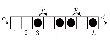
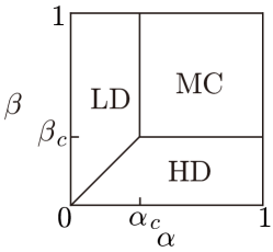
Figure 2: Definition of the TASEP (left) and its exact phase diagram for the parallel update (right). The critical points are $\alpha_{c}=\beta_{c}=1-\sqrt{1-p}$.

Varying the boundary parameters $\alpha$ and $\beta$ (with $p$ fixed), one can distinguish three phases (Fig. 2), namely the Low-Density (LD), High-Density (HD) and Maximal-Current (MC) phases. In the LD phase the current $J=p\langle n_{j}(1-n_{j+1})\rangle$ through the system depends only on the input probability $\alpha$. The input is less efficient than the transport in the bulk of the system or the output and therefore dominates the behavior of the whole system. In the HD phase the output is the least efficient part of the system. Therefore the current depends only on the output probability $\beta$. In the MC phase, input and output are more efficient than the transport in the bulk of the system. Here the current has reached the maximum of the fundamental diagram, i.e. the relation between density and current, depending on the update rules.

The phase diagram of the TASEP was firstly derived rigorously in the works [14, 15] for the continuous-time case. In particular, the authors of [15] introduced matrices to construct the exact stationary solution. The basic idea is to make a matrix product with replacing occupied and unoccupied sites by matrices. This matrix product Ansatz has been widely applied to many one-dimensional interacting particle systems [12]. The matrix product representation for the TASEP with parallel update was found in [16] .

4 Exclusive queueing process

The Exclusive Queueing Process (EQP) is defined on a semi-infinite chain where sites are labeled by natural numbers from right to left (Fig. 3). The dynamics of the model is defined as follows:

(i)

input: A new particle is inserted with probability $\alpha$ on the site just behind the last particle in the queue. If there is no particle in the system, a new particle is inserted directly to the site 1 with the same probability.

(ii)

hopping: Particles behind an empty site move forward with probability $p$

(iii)

output: A particle at site 1 is serviced (i.e. removed) with probability $\beta$.

For the parallel update these rules are applied simultaneously to all sites. In the case of backward-sequential update, first (i) and (iii) are carried out. Then (ii) is applied sequentially to all sites starting at site $j=1$. The dynamics of the particle hopping is the same as in the TASEP reviewed in Sec. 3.

We define the length $L$ of the system as the position of the last particle, and thus a new particle is inserted at site $L+1$. Note that this boundary condition for the left end (i) is different from the TASEP case, whereas (iii) is the same. Therefore the EQP can be interpreted as a TASEP of variable length.

The EQP is formulated as a discrete-time Markov process on the state space

$$S=\{\emptyset,1,10,11,100,101,110,111,1000,\dots\},$$ (10)

where $0$ and $1$ correspond to unoccupied and occupied sites. The symbol $\emptyset$ denotes the state in which there is no particle in the queue. In the generic case, the EQP is an irreducible and aperiodic process.

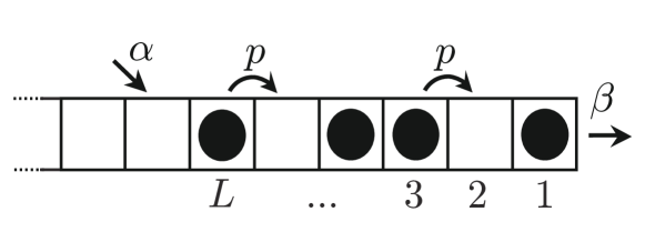
Figure 3: Definition of the Exclusive Queueing Process (EQP). The length $L$ is defined by the position of the last (leftmost) particle.

By changing the input and output probabilities $\alpha$ and $\beta$ the EQP shows boundary-induced phase transitions, which are classified according to different criteria:

• Queueing classification – convergent or divergent queue length (see Sec. 5).
  For the parallel update this classification can be done by constructing exact stationary measure. In the Convergent (C) phase the average system length converges to a finite value as $t\to\infty$. In the Divergent (D) phase, the average length grows infinitely, being proportional to time $t$. We are interested in how the phase diagram of the M/M/1 case (Fig. 1) is changed due to the excluded-volume effect. In Sec. 6, for the special case $p=1$, we see that a generating function of probabilities at each time step allows us to rigorously compute the asymptotic behaviors [18].

• TASEP classification – form of the outflow (see Sec. 7) [19].
  By definition, the inflow of particles is given by $\alpha$. On the other hand, the outflow is not identical to $\beta$ because the last site (server) can be empty. The form of the non-stationary flow $J_{\text{out}}$ is identical to the form for the MC or HD phases of the open TASEP . In the maximal current phase, the current $J_{\text{out}}$ of particles going through the right end is independent of both $\alpha$ and $\beta$. In the high-density phase the current depends on $\beta$, but is independent of $\alpha$.

• Classification according to density profile (see Sec. 8).
  The divergent phase can be divided into subphases according to the number of plateaus in the density profile [20]. The rescaled profile has the form of a rarefaction wave [11].

4.1 Limits and special cases

The discrete-time EQPs have several known models as special cases or limits. The following diagram illustrates the relations between the various models:

$$\begin{CD}{\rm\framebox{Parallel EQP}}@>{\displaystyle\Delta s\to 0}>{}>{\rm\framebox{Continuous EQP}}@<{\displaystyle\Delta s\to 0}<{}<{\rm\framebox{Backward EQP}}\\ @V{\displaystyle p=1}V{}V@V{\displaystyle p\to\infty}V{}V@V{\displaystyle p=1}V{}V\\ {\rm\framebox{ Rule 184 }}@>{\displaystyle\Delta s\to 0}>{}>{\rm\framebox{Continuous M/M/1}}@<{\displaystyle\Delta s\to 0}<{}<{\rm\framebox{Discrete M/M/1}}.\end{CD}$$

Here we consider the continuous-time limit $\Delta s\to 0$ in the master equations, which is taken as follows. We replace $t+1$ by $t+\Delta s$, so that $\Delta s$ is the length of the discrete time step, and the parameters $\alpha$, $\beta$ and $p$, and time $t$ by $\alpha\Delta s$, $\beta\Delta s$ and $p\Delta s$, respectively. In the continuous time processes, the parameters $\alpha$, $\beta$ and $p$ are transition rates.

The special case of the parallel EQP with $p=1$ is the rule 184 cellular automaton. Even though the hopping is deterministic, this case is not classified into the ordinary queueing theory, since particles are still prohibited to jump if the preceding site is occupied. On the other hand, the backward EQP with $p=1$ is the M/M/1 queueing process with discrete time. The continuous-time M/M/1 queueing process is obtained by formally taking the limit $p\to\infty$.

4.2 Explicit probabilities

To close this section, we write down transition probabilities for a few configurations with small $L$ and probabilities for a few times steps. We only consider the simplest case, i.e. parallel update with $p=1$, but this is a good exercise to understand the dynamics of the EQP. In Fig. 4, we use short-hand notations $\alpha^{\prime}=1-\alpha,\beta^{\prime}=1-\beta$, and the arrows with dashed lines correspond to the transitions coming from or going to states with length $L\geq 4$. We notice that no arrow is directed to configurations containing a sequence 00, which is a consequence of the deterministic hopping. Thus this special case is not irreducible on $S$. We restrict our consideration to the subset $\tilde{S}=\{\tau\in S|\tau$ contains no 00$\}$ such that the process is irreducible. Let us start the process at $\emptyset$ at time $t=0$, i.e. $P_{0}(\emptyset;0)=1$ and $P_{0}(\tau;0)=0$ for $\tau\neq\emptyset$. At the next time $t=1$ we have

$$P(\emptyset;1)=(1-\alpha)P(\emptyset;0)=1-\alpha\,,\qquad P(1;1)=\alpha P(\emptyset;0)=\alpha\,,$$ (11)

and then at $t=2$ we have

$$P(\emptyset;2)=(1-\alpha)P(\emptyset;1)+(1-\alpha)\beta P(1;1)=(1-\alpha)(1-\alpha+\alpha\beta)\,,$$ (12)

etc. In principle, one can calculate all the probabilities at any time $t$ recursively. Table 1 provides probabilities for $t=2,3,4$. In the case of the parallel EQP with $p=1$, a matrix product form gives probabilities for each time step (Sec. 6).

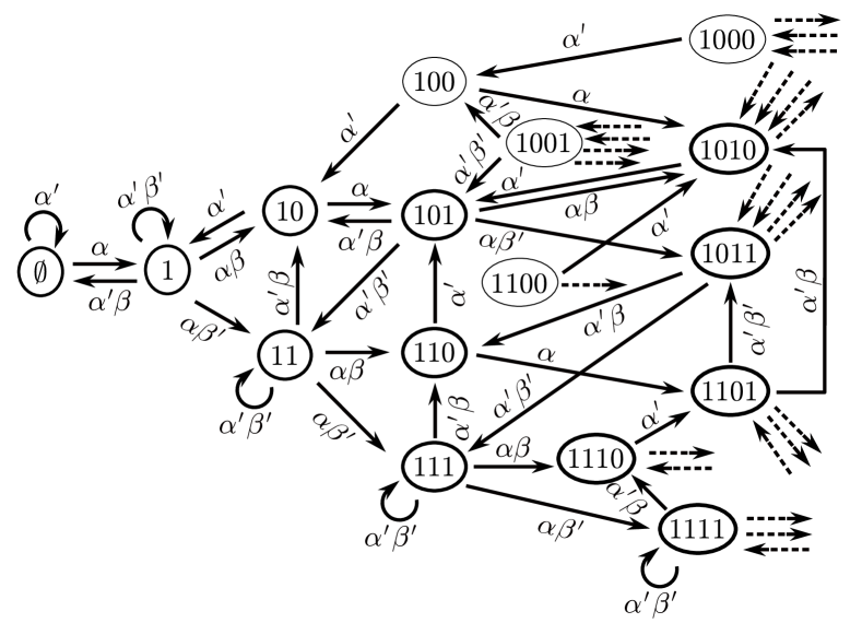
Figure 4: Transition probabilities of a special case of the parallel EQP with update with deterministic hopping ($p=1$) i.e. rule 184. The bold (thin) ellipses are elements of $\tilde{S}$ (resp. $\tilde{S}\backslash S$).

$t$	2	3	4
$\emptyset$	$\alpha^{\prime}(\alpha^{\prime}+\alpha\beta)$	$\alpha^{\prime 2}(2\alpha\beta+\alpha^{\prime}$	$\alpha^{\prime 2}(2\alpha^{2}\beta^{2}+3\alpha\beta\alpha^{\prime}+\alpha^{\prime 2}$
		$+\alpha\beta\beta^{\prime})$	$+2\alpha\beta\alpha^{\prime}\beta^{\prime}+\alpha\beta\alpha^{\prime}\beta^{\prime 2})$
1	$\alpha\alpha^{\prime}(1+\beta^{\prime})$	$\alpha\alpha^{\prime}(2\alpha\beta+\alpha^{\prime}$	$\alpha^{2}\alpha^{\prime}\beta(3\alpha\beta+\alpha^{\prime}+5\alpha\beta\beta^{\prime}$
		$+\alpha^{\prime}\beta^{\prime}+\alpha^{\prime}\beta^{\prime 2})$	$+\alpha^{\prime}\beta^{\prime}+\alpha^{\prime}\beta^{\prime 2}+\alpha^{\prime}\beta^{\prime 3})$
10	$\alpha^{2}\beta$	$\alpha^{2}\alpha^{\prime}\beta(1+2\beta^{\prime})$	$\alpha^{2}\alpha^{\prime}\beta(3\alpha\beta+\alpha^{\prime}+2\alpha^{\prime}\beta^{\prime}+3\alpha^{\prime}\beta^{\prime 2})$
11	$\alpha^{2}\beta^{\prime}$	$\alpha^{2}\alpha^{\prime}\beta^{\prime}(1+2\beta^{\prime})$	$\alpha^{2}\alpha^{\prime}\beta(3\alpha\beta+\alpha^{\prime}+2\alpha^{\prime}\beta^{\prime}+3\alpha^{\prime}\beta^{\prime 2})$
101	0	$\alpha^{3}\beta$	$\alpha^{3}\alpha^{\prime}\beta(1+3\beta^{\prime})$
110	0	$\alpha^{3}\beta\beta^{\prime}$	$\alpha^{3}\alpha^{\prime}\beta\beta^{\prime}(1+3\beta^{\prime})$
111	0	$\alpha^{3}\beta^{\prime 2}$	$\alpha^{3}\alpha^{\prime}\beta^{\prime 2}(1+3\beta^{\prime})$
1010	0	0	$\alpha^{4}\beta^{2}$
1011	0	0	$\alpha^{4}\beta\beta^{\prime}$
1101	0	0	$\alpha^{4}\beta\beta^{\prime}$
1110	0	0	$\alpha^{4}\beta\beta^{\prime 2}$
1111	0	0	$\alpha^{4}\beta^{\prime 3}$

Table 1: Probabilities of finding configurations at first few time steps for the rule 184 case.

5 Convergent and divergent phases

For the parallel EQP the stationary measure has the following matrix product form, which provides the grand canonical ensemble of the parallel-update TASEP with open boundaries, as explained in Sec. 3, with $\alpha=1$:

$$P_{st}(\emptyset) = 1\,,$$ (13)

$$P_{st}(1\tau_{L-1}\dots\tau_{1}) = \left(\frac{\alpha}{p(1-\alpha)}\right)^{L}\langle W|DX_{\tau_{L-1}}\cdots X_{\tau_{1}}|V\rangle\,.$$ (14)

where $\frac{\alpha}{p(1-\alpha)}$ plays a role of a fugacity. The matrices $X_{1}=D$ and $X_{0}=E$, the row vector $\langle W|$ and the column vector $|V\rangle$ should satisfy quartic algebraic relations which are identical to those for the parallel-update TASEP with open boundaries and $\alpha=1$ [16]. The matrix product form (13) allows to use some exact results obtained for the parallel TASEP. The representations of the matrices and vectors are, in general, infinite-dimensional [16]. For the special case $p=1$, the matrices and vectors have two dimensional representation:

$$D=\left(\begin{array}[]{cc}1/\beta-1&0\\ 1/\sqrt{\beta}&0\end{array}\right),\ E=\left(\begin{array}[]{cc}0&1/\sqrt{\beta}\\ 0&0\end{array}\right),\ \langle W|=\left(1\ \sqrt{\beta}\right),\quad|V\rangle=\left(\begin{array}[]{c}1\\ \sqrt{\beta}\end{array}\right).$$ (21)

On the other hand, by taking continuous-time limit we obtain the matrix product stationary measure for the continuous-time EQP [3], whose algebra corresponds to the continuous-time TASEP with open boundaries [15].

As far as we know, a physical interpretation of the grand-canonical ensemble to a process with varying system length was firstly shown in [21]. A similar construction i.e. a matrix product with fugacity, is also possible for a simple model of microtubule growth [22, 23, 24]. However, this is not always true for all TASEPs with varying length. For example the EQP with the backward update, a matrix product form has not been found, although the open TASEP with backward update has a matrix product stationary state [25, 26, 27]. In the recent work [28], a queueing process with two types of customers was introduced, which is called Prioritizing Exclusion Process (PEP). High priority customers can overtake low priority customers. This is another variant of the TASEP with varying system length, by regarding high- and low-priority customers as particles and empty sites, respectively. However, a matrix product stationary measure for the PEP has not been found up to now.

For the parallel EQP, the series

$$Z=\sum_{\tau\in S}P_{st}(\tau)=1+\sum_{L\geq 1}\left(\frac{\alpha}{p(1-\alpha)}\right)^{L}\langle W|D(D+E)^{L-1}|V\rangle$$ (22)

converges, when the condition

$$\begin{cases}\alpha\leq\alpha_{c}=\frac{1-\sqrt{1-p}}{2}&\text{for }\beta>\beta_{c}=1-\sqrt{1-p},\\ \alpha<\alpha_{c}=\frac{\beta(p-\beta)}{p-\beta^{2}}&\text{for }\beta\leq\beta_{c}\end{cases}$$ (23)

is satisfied [29, 16]. The existence of the stationary distribution $\frac{1}{Z}P_{st}(\tau)$ guaranties that we will approach to it, starting from any initial state. In the region $\alpha<\alpha_{c}$ (convergent phase), the average system length $\langle L_{t}\rangle$ and the average number of particles $\langle N_{t}\rangle$ converge to

$$\langle L_{\infty}\rangle=\frac{\alpha p(R-p+2(1-\alpha))}{R(R-p+2(1-\alpha)\beta)},\quad\langle N_{\infty}\rangle=\frac{\alpha(1-\alpha)(p-2\alpha p+R)}{R(R-p+2(1-\alpha)\beta)}$$ (24)

with $R=\sqrt{p(p-4\alpha(1-\alpha))}$. Oppositely, for $\alpha>\alpha_{c}$ (divergent phase) and for $\alpha=\alpha_{c}$ (critical line), $\langle L_{t}\rangle$ and $\langle N_{t}\rangle$ diverge. On the straight-line part of the critical line $\alpha=\alpha_{c}$ ($\beta>1-\sqrt{1-p}$), there are distributions of the system length and the number of particles, but their averages diverge. When $p=1$, the condition (23) simplifies to

$$\alpha<\alpha_{c}=\frac{\beta}{1+\beta}.$$ (25)

As we mentioned, we could not find an exact stationary measure for the backward case. Thus the determination of the phase diagram has to be done by Monte Carlo simulations. The region where the average system length converges is expected to be

$$\begin{cases}\alpha\leq\alpha_{c}=\frac{(1-\sqrt{1-p})^{2}}{p}&(\beta_{c}<\beta<1),\\ \alpha<\alpha_{c}=\frac{\beta(p-\beta)}{p(1-\beta)}&(0<\beta\leq\beta_{c}).\end{cases}$$ (26)

For the backward case, explicit forms of the average values like (24) are unknown except for the special case $p=1$.

6 Dynamics for deterministic hopping

In the case of parallel dynamics, an exact time-dependent solution is also known for deterministic hopping $p=1$ in the bulk [18].

For the deterministic hopping case, an exact expression of the “dynamical state” is possible; starting from the empty chain $\emptyset$ at $t=0$, the probability $P(\tau;t)$ of finding a state $\tau$ at time $t$ can be written as

$$P(\emptyset;t) =\oint\frac{dz}{2\pi iz^{t+1}}\frac{1-\Lambda}{1-z},$$ (27)

$$P(\tau_{L}\cdots\tau_{1};t) =\langle W|X_{\tau_{L}}\cdots X_{\tau_{1}}|V\rangle\beta^{L}\oint\frac{dz}{2\pi iz^{t+1}}\frac{1-\Lambda}{1-z}\Lambda^{L}$$ (28)

with the same matrices and vectors as for the stationary case (21), and the fugacity $\Lambda=\frac{1-\alpha^{\prime}\beta^{\prime}z-\sqrt{(1-\alpha^{\prime}\beta^{\prime}z)^{2}-4\alpha\alpha^{\prime}\beta z^{2}}}{2\alpha^{\prime}\beta z}$. The contour integral picks up the coefficient of $z^{t}$ in the power series of $\frac{1-\Lambda}{1-z}\Lambda^{L}$. This simple form is due to the simplification of the master equation in the special case $p=1$, see [18] for details.

The probability of finding the length $L$ at time $t$ is given as $\oint\frac{dz}{2\pi iz^{t+1}}\frac{1-\Lambda}{1-z}\Lambda^{L}$, since $\langle W|D(D+E)^{L-1}|V\rangle\beta^{L}=1$. Thus the average length of the system at time $t$ and its asymptotic behaviors ($t\to\infty$) are given by

$$\langle L_{t}\rangle=\oint\frac{dz}{2\pi iz^{t+1}}\frac{\Lambda}{(1-z)(1-\Lambda)}\simeq\left\{\begin{array}[]{ll}\frac{\alpha}{\beta-\alpha-\alpha\beta}&\quad(\alpha<\frac{\beta}{1+\beta}),\\ 2\sqrt{\frac{\beta t}{\pi(1+\beta)}}&\quad(\alpha=\beta),\\ (\alpha-\beta+\alpha\beta)t&\quad(\alpha>\frac{\beta}{1+\beta}).\end{array}\right.$$ (32)

The probability of finding $N$ particles at time $t$ is given as $\oint\frac{dz}{2\pi iz^{t+1}}\frac{1-\Lambda}{(1-z)}$ (for $N=0$) and $\oint\frac{dz}{2\pi iz^{t+1}}\frac{\Lambda(1-\Lambda)(1+\beta\Lambda)}{(1-z)}[\Lambda(1-\beta+\beta\Lambda)]^{N-1}$ (for $N\geq 1$). The average number of particles at time $t$ and its asymptotic behavior ($t\to\infty$) can be also calculated as

$$\begin{split}\langle N_{t}\rangle=\oint\frac{dz}{2\pi iz^{t+1}}\frac{\Lambda}{(1-z)(1-\Lambda)(1+\beta\Lambda)}\end{split}\simeq\left\{\begin{array}[]{ll}\frac{\alpha(1-\alpha)}{\beta-\alpha-\alpha\beta}&\ \ (\alpha<\frac{\beta}{1+\beta}),\\ 2\sqrt{\frac{\beta t}{\pi(1+\beta)^{3}}}&\ \ (\alpha=\frac{\beta}{1+\beta}),\\ \frac{\alpha-\beta+\alpha\beta}{1+\beta}t&\ \ (\alpha>\frac{\beta}{1+\beta}).\end{array}\right.$$ (36)

The asymptotic behaviors on the critical line are diffusive (i.e. $\sim t^{1/2}$) as the symmetric random walk. For general $p$, however, more complicated behavior is observed (see Sec. 9).

7 The outflow

Let us consider the non-stationary properties of the EQP in order to derive the phase diagram based on physical arguments. This heuristic understanding of the phase diagram is similar to the open TASEP case, where a domain wall between a low- and high-density regions ($\rho_{\text{left}}$ and $\rho_{\text{right}}$, respectively) moves with velocity [30]

$$v_{s}=\frac{J(\rho_{\text{left}})-J(\rho_{\text{right}})}{\rho_{\text{left}}-\rho_{\text{right}}}.$$ (37)

Here the fundamental diagram $J=J(\rho)$ depends on the update rule [26, 27].

For the EQP, from the particle conservation law, we have

$$\langle N_{t}\rangle=(J_{\text{in}}-J_{\text{out}})t+\langle N_{0}\rangle$$ (38)

Here we assume the outflow $J_{\text{out}}$ is a constant. On the other hand, the inflow $J_{\rm in}$ is always $\alpha$, which is due to the fact that the site where particles enter is by definition never blocked.

From Monte Carlo simulations, we find the outflow $J_{\text{out}}$ as

$$J_{\text{out}}=\begin{cases}\frac{\beta(p-\beta)}{(p-\beta^{2})}&\quad(\beta\leq\beta_{c}),\\ \frac{(1-\sqrt{1-p})}{2}&\quad(\beta>\beta_{c}),\end{cases}$$ (39)

for the parallel case and

$$\quad J_{\text{out}}=\begin{cases}\frac{\beta(p-\beta)}{p(1-\beta)}&\ (\beta\leq\beta_{c}),\\ \frac{(1-\sqrt{1-p})^{2}}{p}&\ (\beta_{c}<\beta).\end{cases}$$ (40)

for the backward case. According to the TASEP explained in Sec. 4 these phases might be called High-Density (HD) phase for $\beta\leq\beta_{c}$ and Maximal-Current (MC) phase for $\beta_{c}<\beta$. Note that the form of the outflow is identical to the critical value $\alpha_{c}$ as given in Equations (23) and (26). The phase diagram is now understood as follows: when $J_{\text{in}}<J_{\text{out}}$ ($J_{\text{in}}>J_{\text{out}}$), the number of particles increases (resp. decreases). The system length also increases (resp. decreases) according to $J_{\text{in}}<J_{\text{out}}$ ($J_{\text{in}}>J_{\text{out}}$), if we assume the “density” $\langle N_{t}\rangle/\langle L_{t}\rangle$ is a constant. We remark that the density profile is not always globally constant, which we will review in the next Section. We also remark that the formula (37) is not satisfied by the “shock” (i.e. the left end of the density profile) in the EQP. After the “shock” reaches the vicinity of the server, the forms (39) and (40) are no longer valid, and the outflow becomes $\alpha$. This means the convergence to the stationary distribution.

So far, based on the queueing and TASEP classifications, we have divided the parameter space into 4 regions, the MC-C, MC-D, HD-C and HD-D phases.

8 Subphases of the divergent phase

Let us consider the situation that the input probability $\alpha$ is much larger than the output probability $\beta$ (e.g. $\alpha=1$). In this case, new particles are always injected to the system, so the density $\rho_{\text{left}}$ near the left end is expected to be 1. On the other hand, the density near the right end is expected to be

$$\rho_{\text{right}}\simeq\begin{cases}\frac{p-\beta}{p-\beta^{2}}&\quad(\beta\leq\beta_{c}),\\ \frac{1}{2}&\quad(\beta>\beta_{c})\end{cases}$$ (41)

for parallel update and

$$\rho_{\text{right}}\simeq\begin{cases}\frac{p-\beta}{p(1-\beta)}&\quad(\beta\leq\beta_{c}),\\ \frac{1-\sqrt{1-p}}{p}&\quad(\beta>\beta_{c})\end{cases}$$ (42)

for backward update. In this section, we review the global density profile that can obtained by “cutting” a rarefaction wave, and we will see that the density 1 near the left end is not always realized. Then we further divide the divergent phases into subphases based on the form of the density profile.

In the TASEP (typically on $\mathbb{Z}$), a rarefaction wave is derived by a hydrodynamic approach [11]: The rescaled density profile $\rho(x=j/t)$ (see Fig. 5)

$$\rho(x)\simeq\begin{cases}\rho_{\rm right}&\qquad(x<f(\rho_{\rm right})),\\ f^{-1}(x)&\qquad(f(\rho_{\rm left})>x>f(\rho_{\rm right})),\\ \rho_{\rm left}&\qquad(x>f(\rho_{\rm left}))\end{cases}$$ (43)

with $f(\rho)=-\frac{dJ}{d\rho}$ does not change the shape (i.e. is “time invariant”) for $\rho_{\rm left}>\rho_{\rm right}$. The fundamental diagram is given as

$$J(\rho)=\begin{cases}\frac{1-\sqrt{1-4p\rho(1-\rho)}}{2}&\qquad(\text{parallel}),\\ \frac{p\rho(1-\rho)}{1-p\rho}&\qquad(\text{backward}).\end{cases}$$ (44)

Thus we find the curved part of the profile, respectively, as

$$f^{-1}(x)=\begin{cases}\frac{1}{2}+\frac{x}{2}\sqrt{\frac{1-p}{p(p-x^{2})}}&\qquad\text{(parallel}),\\ \frac{1}{p}-\frac{1}{p}\sqrt{\frac{1-p}{1+x}}&\qquad\text{(backward}).\end{cases}$$ (45)

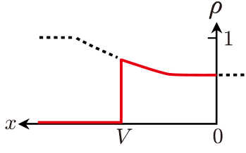
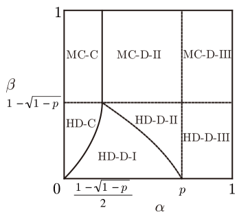
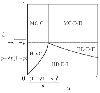
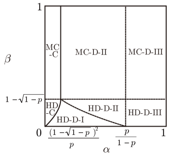
Figure 5: A schematic picture for the density profile in the divergent phase (top-left), where $x$ is the rescaled position $j/t$, and the phase diagrams of the EQP with parallel (top-right) and backward-sequential dynamics for $p<1/2$ (bottom-left) and $p>1/2$ (bottom-right). According to the injection probability (rate) $\alpha$, the rarefaction wave is “cut” by the leftmost particle ($x=V$) and the server ($x=0$). The end of the queue can be in three different regimes, (plateau at density $\rho<1$, regime of increasing density or plateau at density $\rho=1$), which defines the regions I, II, III., respectively. The density profile shown here belongs to II.

We assume that in the divergent phase of the EQP the global density profile $\rho(x)$ can be written as (43) for $0<x<V$, where the velocity $V$ (i.e. $V=\langle L_{t}\rangle/t$) is determined by the particle number conservation: $\int_{0}^{V}\rho(x)dx=\alpha-J_{\text{out}}$. From this assumption, which is supported by simulations, we find

$$V=\begin{cases}\alpha\frac{p-\beta^{2}}{p-\beta}-\beta&\left(\text{I: }\frac{\beta(p-\beta)}{p-\beta^{2}}<\alpha\leq\frac{(p-\beta)^{2}}{p-2p\beta+\beta^{2}}\right),\\ 2p\alpha-p+2\sqrt{p\alpha(1-p)(1-\alpha)}&\left(\text{II: }\max\left(\frac{(p-\beta)^{2}}{p-2p\beta+\beta^{2}},\frac{1-\sqrt{1-p}}{2}\right)<\alpha\leq p\right),\\ \alpha&\left(\text{III: }\quad p<\alpha\leq 1\right),\end{cases}$$ (46)

for the parallel EQP, and

$$V=\begin{cases}\frac{p(1-\beta)}{p-\beta}\alpha-\beta&\left(\text{I: }\frac{\beta(p-\beta)}{p(1-\beta)}<\alpha\leq\frac{(p-\beta)^{2}}{p(1-p)}\right),\\ 2\sqrt{p(1-p)\alpha-p(1-\alpha)}&\left(\text{II: }\max\left(\frac{(p-\beta)^{2}}{p(1-p)},\frac{(1-\sqrt{1-p})^{2}}{p}\right)<\alpha\leq\frac{p}{1-p}\right),\\ \alpha&\left(\text{III: }\frac{p}{1-p}<\alpha\leq 1\right),\end{cases}$$ (47)

for the backward EQP.

To summarize, we have found up to 5 subphases in the divergent case, according to the classification based on the forms of the outflow $J_{\text{out}}$ and the velocity $V$, as shown Fig. 5. The shape of the global density profile changes depending on the parameters.

9 Critical line: Non-universal behavior

In the divergent phase the average length $\langle L_{t}\rangle$ and the average number of particles $\langle N_{t}\rangle$ diverge linearly in time. On the phase transition line separating the convergent and divergent phases the growth is slower than linear, i.e.

$$\langle X_{t}\rangle=O({t^{\gamma_{X}}})\qquad(X=L,N),$$ (48)

where the critical exponents $\gamma_{X}$ are smaller than 1.

Fig. 6 shows the time-dependence of the average system length obtained by Monte Carlo simulations. As one can observe in these log-log plots, the slopes depend both on the update type and the location on the critical line (curved part $\beta<\beta_{c}$ or straight part $\beta>\beta_{c}$). Fig. 7 also provides simulation results of the exponents. Depending on the update rule, the exponents have different values:

parallel: $$\qquad\gamma_{X}=\begin{cases}1/2&(\text{for }\beta<\beta_{c})\\ 1/4&(\text{for }\beta>\beta_{c})\end{cases}$$ (49)

backward: $$\qquad\gamma_{X}=\begin{cases}1/2&(\text{for }\beta<\beta_{c}),\\ g(p)&(\text{for }\beta>\beta_{c},p<p_{c})\\ 0&(\text{for }\beta>\beta_{c},p>p_{c})\end{cases}$$ (50)

with some function $g(p)\in(0,1/4)$, whose explicit form is not known. The nonuniversal behavior (50) and the existence of the critical point $p_{c}$ for the backward case have been tested by simulations ($t\lesssim 10^{6}$, averaged over up to $10^{6}$ samples [31]). We think that this is the most reasonable interpretation, although one could consider other scenarios on the straight part of the critical line $\alpha=\alpha_{c},\beta>\beta_{c}$ for the backward case, e.g. the average length that always converges, but with extremely slow relaxation to the stationary length for small $p$.

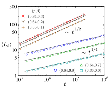
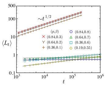
Figure 6: Time-dependence of average system length $\langle L_{t}\rangle$ on the critical line for parallel dynamics (left) and backward dynamics (right).

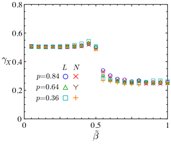
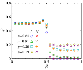
Figure 7: Exponents $\gamma_{X}$ for parallel dynamics (left) and backward dynamics (right). $\beta$ has been rescaled so that $\tilde{\beta}=0,1/2,1$ corresponds to $\beta=0,\beta_{c},1$, respectively.

10 Model extensions

10.1 EQP with Langmuir Kinetics

The TASEP has been extended by including Langmuir Kinetics (TASEP-LK), which is relevant for applications in biology and has a rich phase diagram [32, 33]. In a similar way we have combined the parallel EQP [29] with Langmuir kinetics (EQP-LK).

In the presence of Langmuir kinetics, particles in the bulk are detached with probability $\omega_{D}$, and for each empty site $j(\leq L)$ a particle is attached with probability $\omega_{A}$ (see Fig. 8). As in the TASEP-LK [32, 33], the attachment and detachment probabilities are scaled as $\omega_{A}=\Omega_{A}/L$ and $\omega_{D}=\Omega_{D}/L$ which leads to a competition between bulk and boundary dynamics. We do not impose attachment and detachment when the system length is $0$. Note that, in contrast to the TASEP-LK, the system length $L_{t}$ of the EQP-LK varies, and thus probabilities $\omega_{A},\omega_{D}$ depend on the current state.

In each time step, first the configuration is updated according to the rule of the EQP with parallel update. Then the Langmuir kinetics is applied. This defines the EQP-LK with parameters $(p,\alpha,\beta,\Omega_{A},\Omega_{D})$, which reduces to the EQP for $\Omega_{A}=\Omega_{D}=0$. The EQP-LK can be interpreted as an effective model for interacting queues where the attachment and detachment corresponds to customers changing from and to other queues, respectively. Thus the other queues are considered to act as reservoir for the EQP-LK.

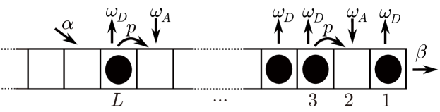
Figure 8: Exclusive queueing process with Langmuir kinetics.

Preliminary studies have found that the EQP-LK has surprising properties [34, 35, 36]. It shows a strong dependence of the behavior on the initial condition, see Fig. 9. In fact, in a certain parameter region, some samples appear to converge to a finite length whereas other samples appear to diverge (within the simulation time), see Fig. 10. The percentage of apparently divergent samples depends strongly on the initial length $L_{0}=L_{t=0}$ of the queue. It is very small for small $L_{0}$ and becomes large for large $L_{0}$.

This surprising behavior is related to the length dependence of the attachment and detachment probabilities. Once the queue has become short it is difficult to escape from $L_{t}=0$ after reaching $L_{t}=0$ since the detachment rate is large. Thus, starting from a short queue $L_{0}<L^{*}$, the length tends to remain finite. On the other hand, starting from long queues $L_{0}>L^{*}$ the chain tends to grow further because the detachment rate is small. These two observations contradict the general theory of Markov processes. However, we can interpret the convergence from short queues as “quasi stationary,” and it is required very long time to reach e.g. $L=500$, which is probably impossible to realize in our computer environment, see some observations on the first passage time [36]. In this sense, the ergodicity of the EQP-LK is effectively broken. In other words, there is a very high maximum of the “potential” in a certain point $L=L^{*}$. This is opposite property to a microtubule model [22], where the length can be regulated around $L^{*}$.

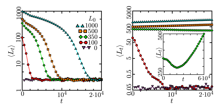
Figure 9: Behavior of $\langle L_{t}\rangle$ starting from various initial lengths, for $(p,\alpha,\beta,\Omega_{A},\Omega_{D})=(0.8,0.2,0.2,0.2,0.35)$ (left) and $(p,\alpha,\beta,\Omega_{A},\Omega_{D})=(0.8,0.3,0.2,0.1,0.9)$ (right). We have set the initial density as $\Omega_{A}/(\Omega_{D}+\Omega_{A})$, and averaged over $10^{3}$ samples. In (a), all the average lengths with initial lengths $L_{0}=0,100,350,500,1000$ converge to a stationary value. In (b), we find that the behavior of the average length depends on the initial length. Furthermore in the inset of (b), the length exhibits non-monotonic behavior.

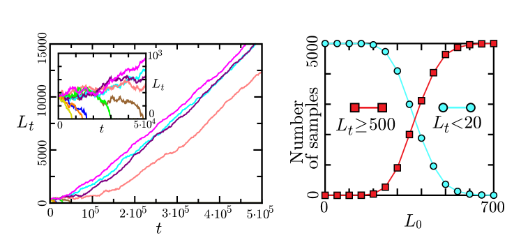
Figure 10: (Left) Behavior of $L_{t}$ for 9 individual samples. The parameters were set as $(p,\alpha,\beta,\Omega_{A},\Omega_{D})=(0.8,0.3,0.2,0.1,0.9)$, and every sample started from the length $L_{0}=350$ and the density $\Omega_{A}/(\Omega_{A}+\Omega_{D})=0.9$. (Right) Distribution of the system length $L_{t}$ at $t=2\cdot 10^{5}$ obtained from $5\cdot 10^{3}$ simulation samples with the same parameter setting and various initial lengths $L_{0}$.

10.2 Multi-chain EQPs

The EQP-LK is a single-chain queueing process that can be interpreted as an effective model for a multi-chain process. The interaction between the chains through exchange of particles is modeled through Langmuir kinetics which allows the change of the particle number within the bulk of the queue.

Of course, the EQP can also be extended to a genuine multi-chain model. For applications, 2-chain models are of special interest. As a model for a bottleneck on a highway, a configuration as in Fig. 11 can be used. Here particles can only change with probability $q$ from chain 2 to chain 1 on sites $j=1,\ldots,M$ where $M$ is a fixed parameter. For sites $j>M$ such a change is not allowed. Otherwise, the bulk and input dynamics (with parameters $p_{1},p_{2}$ and $\alpha_{1},\alpha_{2}$, respectively) are identical to that of a single EQP. However, only particles at position $j=1$ of chain 1 are serviced.

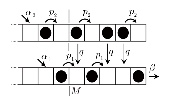
Figure 11: 2-chain EQP for a highway bottleneck. The bulk dynamics of each chain is that of the standard EQP. In a finite region ($j=1,2,\ldots,M$) particle changes from chain 2 (top) to chain 1 (bottom) are allowed.

11 Applications and related models

Originally, queueing theory was developed mainly for applications in telecommunications. Nowadays, however, it is a standard approach in various fields, ranging from supply chains [37] to traffic flow and biology.

The most natural application of the EQP is queueing of pedestrians, e.g. at a supermarket checkout. This can be generalized in a straightforward way to multiple queues where customers might jump from one queue to another. A generalization where the probability of moving depends on the gap to the next customer in front was studied in [38]. This might be realistic e.g. for queues at an airport check-in where the passingers have to pick up their luggage when moving forward. Since this is uncomfortable they typically wait until a critical gap to the preceding passenger has opened.

One advantage of the EQP and its relatives for applications is that it is an intrinsically microscopic model where the different “units” can be distinguished. Therefore they can have different properties (e.g. average velocities) in a natural way.

In the context of vehicular traffic, various queueing based models have been proposed, e.g. [39, 40, 41, 42, 43, 44]. Even the cell transmission model [45] might be interpreted as queueing model. Often these models are used to study traffic on networks where links correspond to roads or road sections and nodes to intersections which are characterized by a service rate. In contrast, in the model developed in [43] the trajectories of the vehicles are related to a M/M/1 queue by identifying space in the traffic model with time in the queueing model.

Other variants of the TASEP on a lattice of varying length have been proposed as applications to biological systems. In [46, 47, 48, 49] the dynamically extending exclusion process (DEEP) has been introduced as a model for fungal growth. In the DEEP not all particles are removed from the system as they reach the end, but with some probability form a new lattice site. In contrast to the EQP, the DEEP has no mechanism for reducing the system length and therefore the length of the system is always diverging. Microtubules [50] are the analogues of highways in cells. However, their lengths are not constant, but changes dynamically. The mechanism of length regulation of microtubules has been investigated in [51, 22] using a variant of the TASEP where the first (output) site can be removed or attached under certain conditions. Similar models have been used to describe bacterial flagellar growth [52]. In [22], a condition on parameters for the convergence of a simplified model of mictrotubules is discussed. This can be also rigorously derived by constructing a stationary measure in a similar form to that of the EQP (14) [23].

12 Discussion

The Exclusive Queueing Process (EQP) can be considered as a minimal model of pedestrian queues which takes into account the internal dynamics of the queue. We have found that the EQP has a rich phase diagram. Surprisingly, it shows a strong dependence of its critical properties on the update scheme. This is rather different from the TASEP with a fixed system length. The order of the phase transition between the diverging and converging phases can also be different.

Besides application to pedestrian queues and vehicular traffic, variants of the EQP have interesting applications to biological processes like fungal growth and microtubule length regulation. We expect that transport models with varying system lengths will show many other interesting phenomena.

References

- [1] J. Medhi: Stochastic Models in Queueing Theory, Academic Press, San Diego 2003)
- [2] T.L. Saaty: Elements of Queueing Theory With Applications, Dover Publ. (1961)
- [3] C. Arita: Phys. Rev. E 80, 051119 (2009)
- [4] D. Yanagisawa, A. Tomoeda, R. Jiang, K. Nishinari: JSIAM Lett. 2, 61 (2010)
- [5] A.K. Erlang: Nyt Tidsskrift for Matematik B 20, 33 (1909)
- [6] Rinaldo B. Schinazi, Classical and Spatial Stochastic Process , Birkhäuser
- [7] T.M. Liggett: Stochastic Interacting Systems: Contact, Voter and Exclusion Processes, Springer, New York (1999)
- [8] G.M. Schütz, in Phase Transitions and Critical Phenomena vol 19., C. Domb and J. L. Lebowitz Ed., Academic Press, San Diego (2001)
- [9] R. K. P. Zia and B. Schmittmann, J. Stat. Mech. (2007) P07012
- [10] A. Schadschneider, D. Chowdhury, K. Nishinari: Stochastic Transport in Complex Systems: From Molecules to Vehicles, Elsevier Science, Amsterdam (2010)
- [11] P.L. Krapivsky, S. Redner, E. Ben-Naim: A Kinetic View of Statistical Physics, Cambridge University Press, Cambridge (2010)
- [12] R.A. Blythe, M.R. Evans: J. Phys. A: Math. Gen. 40, R333 (2007)
- [13] B. Derrida: J. Stat. Mech. (2007) P07023
- [14] G. Schütz, E. Domany: J. Stat. Phys. 72, 277 (1993)
- [15] B. Derrida, M. R. Evans, V. Hakim, V. Pasquier: J. Phys. A 26, 1493 (1993)
- [16] M.R. Evans, N. Rajewsky, E.R. Speer: J. Stat. Phys. 95, 45 (1999)
- [17] J. de Gier, B. Nienhuis: Phys. Rev. E59, 4899 (1999)
- [18] C. Arita, A. Schadschneider: Phys. Rev. E 84, 051127 (2011)
- [19] C. Arita, A. Schadschneider: Phys. Rev. E 83, 051128 (2011)
- [20] C. Arita, A. Schadschneider: J. Stat. Mech. (2012) P12004
- [21] O.J. Heilmann: J. Stat. Phys. 116, 855 (2004)
- [22] A. Melbinger, L. Reese, E. Frey: Phys. Rev. Lett. 108, 258104 (2012)
- [23] C. Arita, A. T. Lück, L. Santen: in progress.
- [24] A. T. Lück: Master Thesis, University of Saarland (2014)
- [25] M.R. Evans: J. Phys. A 30, 5669 (1997)
- [26] N. Rajewsky, A. Schadschneider, M. Schreckenberg: J. Phys. A 29, L305 (1996)
- [27] N. Rajewsky, L. Santen, A. Schadschneider, M. Schreckenberg: J. Stat. Phys. 92, 151 (1998)
- [28] J. de Gier and C. Finn: arXiv:1403.5322
- [29] C. Arita, D. Yanagisawa: J. Stat. Phys. 141, 829 (2010)
- [30] A.B. Kolomeisky, G.M. Schütz, E.B. Kolomeisky, J.P. Straley: J. Phys. A: Math. Gen. 31, 6911 (1998)
- [31] C. Arita, A. Schadschneider: EPL 104, 30004 (2013)
- [32] A. Parmeggiani, T. Franosch, and E. Frey, Phys. Rev. Lett. 90, 086601 (2003)
- [33] M. R. Evans, R. Juhász, L. Santen Phys. Rev. E 68, 026117 (2003)
- [34] C. Schultens: Bachelor Thesis, Cologne University (2012)
- [35] C. Borghardt: Bachelor Thesis, Cologne University (2012)
- [36] C. Arita, A. Schadschneider et al.: in preparation
- [37] W.J. Hopp, M.L. Spearman: Factory Physics, McGraw-Hill, Boston (2008)
- [38] C. Behlau: Bachelor Thesis, Cologne University (2013)
- [39] D. Heidemann: Transp. Sci. 35, 405 (2001)
- [40] N. Eissfeldt, J. Gräfe, P. Wagner: Transp. Res. Rec. Board (2003)
- [41] D. Helbing: J. Phys. A: Math. Gen. 36, L593 (2003)
- [42] T. van Woensel, N. Vandaele: Asia-Pacific J. Operat. Res. 24, 435 (2007)
- [43] F.C. Cáceres, P.A. Ferrari, E. Pechersky: J. Stat. Mech. (2007) P07008
- [44] J. MacGregor Smith, F.R.B. Cruz: Physica A 395, 560 (2014)
- [45] C. Daganzo: Transp. Res. B 28, 269 (1994)
- [46] K. Sugden, M.R. Evans, W.C.K. Poon, N.D. Read: Phys. Rev. E 75, 031909 (2007)
- [47] K. Sugden and M.R. Evans, J. Stat. Mech. (2007) P11013
- [48] M.R. Evans and K.E.P. Sugden, Physica A 384, 53 (2007)
- [49] S. Dorosz, S. Mukherjee, T. Platini: Phys. Rev. E 81, 042101 (2010)
- [50] J. Howard: Mechanics of Motor Proteins and the Cytoskeleton, Sinauer Associates (2001)
- [51] D. Johan, C. Erlenkämper, K. Kruse: Phys. Rev. Lett. 108, 258103 (2012)
- [52] M. Schmitt, H. Stark: EPL 96, 28001 (2011)