Efficiency statistics at all times: Carnot limit at finite power

Abstract

We derive the statistics of the efficiency under the assumption that thermodynamic fluxes fluctuate with normal law, parametrizing it in terms of time, macroscopic efficiency, and a coupling parameter $\zeta$. It has a peculiar behavior: No moments, one sub- and one super-Carnot maxima corresponding to reverse operating regimes (engine/pump), the most probable efficiency decreasing in time. The limit $\zeta\to 0$ where the Carnot bound can be saturated gives rise to two extreme situations, one where the machine works at its macroscopic efficiency, with Carnot limit corresponding to no entropy production, and one where for a transient time scaling like $1/\zeta$ microscopic fluctuations are enhanced in such a way that the most probable efficiency approaches Carnot at finite entropy production.

Efficiency quantifies how worth a local gain at the expense of a global loss is. In thermodynamics, “losses” are measured by the rate $\bar{\sigma}_{2}>0$ at which entropy is externalized to the environment in the form of a degraded form of energy, while “gain” is the rate $-\bar{\sigma}_{1}$ at which entropy is expelled from a system to upgrade its own state. Globally, entropy is produced at rate $\bar{\sigma}=\bar{\sigma}_{2}+\bar{\sigma}_{1}$, and the second law of thermodynamics $\bar{\sigma}\geq 0$ conveys that locally one cannot earn more of what is globally lost. Then, the efficiency $\bar{\eta}=-\bar{\sigma}_{1}/\bar{\sigma}_{2}$ is bounded by the (scaled) Carnot efficiency $\eta_{c}=1$. Alas, the craving of this limit is deluded by the fact it occurs at zero power, which is useless for any activity to be accomplished in a reasonable time.

This picture is only tenable for macroscopic systems. For microscopic systems subject to random fluctuations, the concept of a stochastic efficiency has been recently introduced by Verley et al. gatien1 ; gatien2 . The first notion one has to revise is that a fluctuating efficiency can indeed exceed the Carnot limit, when in a machine designed to convert in average a form of input power into a form of output power (e.g. an engine producing work at the expense of a heat flow), for a rare event the input and output are reversed (e.g. a pump that employs mechanical work to absorb heat). Moreover, it has been observed that for time-symmetric protocols in the long time limit the Carnot efficiency becomes the least probable in a “large deviation” sense ld – a very counterintuitive and fascinating result that, in its time-asymmetric variant gatien2 ; gingrich , is already subject to experimental inquiry roldan . Corrections at long finite times have been estimated in Ref. gingrich .

In this work we derive the full probabilit density function (p.d.f.) of the efficiency, under the assumption that thermodynamic fluxes are distributed with multivariate Gaussian with cumulants growing linearly in time. The efficiency p.d.f. displays quite peculiar features. In particular, it does not afford moments of any order, so that there is no average efficiency and mean-square error. Experimentally, this implies that any data analysis should focus on most probable values. About the latter, after an initial transient the distribution becomes bimodal, as observed numerically in Ref. single . As time elapses, the more pronounced maximum drifts towards the always smaller macroscopic value of the efficiency, while a less pronounced maximum at higher efficiency moves in the super-Carnot region towards infinity. We provide a clear physical interpretation of these two peaks. Finally, we argue that the macroscopic framework fails to capture another way of approaching Carnot at finite entropy production, at finite time, when microscopic fluctuations are enhanced so to affect the macroscopic behavior.

Macroscopic nonequilibrium thermodynamics degroot is rooted on two assumptions, both of which are today being challenged in the framework of the stochastic theory of nonequilibrium thermodynamics st1 ; st3 : Certain fluxes $\bm{x}=(x_{1},x_{2})$, with units of an extensive physical quantity per time, take definite values $\bar{\bm{x}}$; Fluxes are linearly related to their conjugate thermodynamic forces $\bm{f}$ via $\bar{\bm{x}}=L\bm{f}$, where the linear response matrix $L$ is assumed to be positive-semidefinite and symmetric by virtue of the Onsager reciprocity relations, yielding a non-negative macroscopic entropy production rate $\bar{\sigma}=\bm{f}\cdot L\bm{f}$.

We relax the first assumption, by supposing that at a given time $t$ fluxes $\bm{x}$ are distributed with law $P_{t}(\bm{x})$. Each current produces entropy at rate $\sigma_{i}=f_{i}x_{i}$, for a total entropy production rate $\sigma=\sigma_{1}+\sigma_{2}$, with units of $k_{B}$ per time. Then, the adimensional efficiency

$$\eta=-\frac{f_{1}x_{1}}{f_{2}x_{2}}=-\frac{\sigma_{1}}{\sigma_{2}}$$ (1)

is a stochastic variable distributed with p.d.f.

$$P_{t}(\eta) = \int dx_{1}dx_{2}\,\delta\left(\eta+\frac{x_{1}f_{1}}{x_{2}f_{2}}\right)P_{t}(x_{1},x_{2})$$ (2)

$$= \varphi\int dx|x|P_{t}\left(-\varphi\eta\,x,x\right),$$

where $\varphi=f_{2}/f_{1}$ can be assumed to be positive. A remarkable fact one immediately encounters is that the efficiency can fluctuate beyond the Carnot limit. The probability of an efficiency higher than Carnot coincides with the probability of negative entropy production rate,

$$P_{t}(\eta<1) = P_{t}({\sigma>0})=\big{\langle}\theta(\sigma)\big{\rangle}_{t}$$ (3a)

$$P_{t}(\eta>1) = P_{t}({\sigma<0})=\big{\langle}\theta(\sigma)e^{-t\sigma}\big{\rangle}_{t},$$ (3b)

where $\theta$ is Heaviside’s step function. The rightmost equations follow from the fluctuation theorem ft ; polespo

$$\frac{P_{t}(\sigma)}{P_{t}(-\sigma)}=e^{t\sigma},$$ (4)

which states that processes producing negative entropy are exponentially disfavored with respect to those producing positive entropy. Therefore, that super-Carnot efficiencies are unlikely compared to sub-Carnot efficiencies is an incarnation of the fluctuation theorem.

Exact results can be obtained by assuming that fluxes are distributed with normal multivariate density function

$$P_{t}(\bm{x})=\frac{t}{4\pi\sqrt{|L|}}\exp\left[-{\frac{t}{4}(\bm{x}-\bar{\bm{x}})\cdot L^{-1}(\bm{x}-\bar{\bm{x}})}\right],$$ (5)

where $|\cdot|$ is the determinant. That (one-half) the correlation matrix should be identified with the linear response matrix is corroborated by the Green-Kubo relations

$$L_{ij}=\frac{t}{2}\langle(x_{i}-\bar{x}_{i})(x_{j}-\bar{x}_{j})\rangle,$$ (6)

another well-known consequence of the fluctuation theorem andrieux . The time dependence in Eq. (5) is due to the fact that the time-integrated fluxes $t\bar{\bm{x}}$ increase linearly in time, and correspondingly so do their cumulants. Under these assumptions the efficiency p.d.f. Eq. (2) can be exactly calculated supp . It only depends on four adimensional parameters: The macroscopic efficiency $\bar{\eta}$, the coupling parameter $\zeta=|L|/(L_{11}L_{22})\in[0,1]$ that for thermoelectric devices benenti is related to the so-called figure of merit $zT=1/\zeta-1$, the average entropy production rate $\bar{\sigma}$, which sets the time scale and can be reabsorbed by a time reparametrization $\tau=t\bar{\sigma}$, and $\epsilon=\pm 1$. Being $\bar{\sigma}$ the only extensive parameter, large $\tau$ stands both for large times and the macroscopic limit. We obtain supp

$$P_{\tau}(\eta)=\frac{e^{-\frac{\tau}{4}}}{\pi a(\eta)\sqrt{|C|}}\left\{1+\sqrt{\pi\tau}\,h(\eta)\,e^{\tau h(\eta)^{2}}\mathrm{\,erf}\,\left[\sqrt{\tau}h(\eta)\right]\right\}$$ (7)

where $\mathrm{erf}$ is the error function and

$$a(\eta) = (1-\eta)^{2}+\frac{1}{|C|}\left(\frac{\eta-\bar{\eta}}{1-\bar{\eta}}\right)^{2}$$ (8a)

$$h(\eta) = \frac{1-\eta}{2\sqrt{a(\eta)}}.$$ (8b)

Here, $|C|=|L|f_{1}^{2}f_{2}^{2}/\bar{\sigma}^{2}$ is the determinant of the matrix with dimensionless entries $C_{ij}=L_{ij}f_{i}f_{j}/\bar{\sigma}$. It can be expressed in terms of our parameters as

$$|C|=\frac{zT}{2}\left(1+\epsilon\sqrt{1-\frac{4}{zT}\frac{\bar{\eta}}{(1-\bar{\eta})^{2}}}\right)-\frac{\bar{\eta}}{(1-\bar{\eta})^{2}},$$ (9)

where $\epsilon=\pm$ accounts for the existence of two probability distributions corresponding to given parameters. For $|L|$ to be real, the known bound

$$\bar{\eta}\leq\frac{1-\sqrt{\zeta}}{1+\sqrt{\zeta}}$$ (10)

must hold benenti . Importantly, $a(\eta)$ is positive semidefinite.

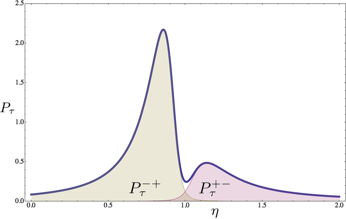
Figure 1: Bold curve: efficiency distribution $P_{\tau}(\eta)$ for parameter values $\zeta=0.01$, $\bar{\eta}=0.6$, $\tau=10$, $\epsilon=+1$. Filled curves beneath: $P^{-+}_{\tau}(\eta)$ and $P^{+-}_{\tau}(\eta)$, showing that each maximum is mostly due to one working mode of the engine.

Let us study the efficiency p.d.f. in detail. First, it is a power-law distribution with tails

$$P_{\tau}(\eta\to\pm\infty)\propto\eta^{-2},$$ (11)

which, after submission of this letter, has been proven to be a universal property of efficiency distributions proesmans . As a consequence, it does not afford finite moments of any order. Hence, the macroscopic efficiency $\bar{\eta}$ is not the average efficiency $\langle\eta\rangle_{t}$, which is not finite.

In Fig. 1 the efficiency distribution is plotted as the bold curve. Remarkably, for a large class of parameters it displays two maxima at $\eta_{m},\eta_{m}^{\ast}$ and a minimum, the latter slightly off the Carnot efficiency. Hence, not only super-Carnot efficiencies are possible, but indeed there appears a local maximum with efficiency higher than Carnot. To understand its physical origin, we distinguish four operational regimes of the machine, according to the signs of the two contributions $\sigma_{1}$ and $\sigma_{2}$ to the entropy production rate. The two regimes contributing to positive efficiencies are the machine $-+$ that employs process 2 flowing along its spontaneous tendency, to drive process 1 against its spontaneous tendency (e.g. heat engine) and the dual machine $+-$ where the system’s spontaneous tendency is used to drive the environment against its tendency (e.g. the heat pump). Correspondingly we have $\theta(\eta)P_{\tau}(\eta)=P^{+-}_{\tau}(\eta)+P^{-+}_{\tau}(\eta)$ where

$$P_{\tau}^{+-}(\eta)=\int_{\begin{subarray}{c}+\sigma_{1}>0\\ -\sigma_{2}>0\end{subarray}}dx_{1}dx_{2}\,P_{t}(x_{1},x_{2})\,\delta\left(\eta+\frac{f_{1}x_{1}}{f_{2}x_{2}}\right)$$ (12)

and similarly for $P_{\tau}^{-+}$. Shaded plots are provided in Fig. 1, showing that each of the two maxima is almost exclusively determined by one of the two modes of the machine, the second of which by inversion of input/output has typical efficiency $1/\eta_{m}^{\ast}<1$. Regimes $++$ and $--$ contribute to the tail of the distribution at $\eta<0$.

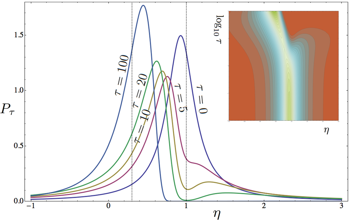
Figure 2: Main frame: Efficiency distribution at various scaled times, for $\zeta=0.05$, $\bar{\eta}=0.3$, $\epsilon=+$. The vertical dotted lines correspond to $\bar{\eta}$ and $\eta_{c}$. Inset: Contour plot of the efficiency p.d.f. as a function of $\eta$ and $\tau$ (in log scale). Maxima are points where the level lines have horizontal tangents. After a critical time, a second maximum drifting to infinity appears.

Let us now study the behavior of $P_{\tau}(\eta)$ in scaled time, depicted in Fig. 2. At $\tau=0$ we obtain a Cauchy distribution, $P_{0}(\eta)=1/\big{[}\pi a(\eta)\sqrt{|C|}\big{]}$, with maximum at $\eta_{0}=-L_{12}f_{1}/(L_{22}f_{2})$. We have $\eta_{0}\geq\bar{\eta}$, and equality can only occur for $|C|=0$. This implies that the most probable efficiency decreases in time towards $\bar{\eta}$. Furthermore, at thermodynamic equilibrium where all the forces vanish, $\bm{f}\to 0$ at finite $\varphi$, it can be shown that $P^{\,\mathrm{eq.}}_{\tau}(\eta)=P_{0}(\eta)$, which means that systems at equilibrium do not evolve. As time elapses a transition to a bimodal distribution occurs, with the super-Carnot maximum drifting to infinity. We can define a critical time $\tau_{\mathrm{c}}$ at which there appears an inflection point in $P_{\tau}(\eta)$. Numerical plots of $\tau_{\mathrm{c}}$ in terms of $\bar{\eta}$ and $c$ show that the critical time is higher the closer to the maximal efficiency and to the loose coupling condition $\zeta\to 1$ supp . Finally, in the long time limit one has $\mathrm{\,erf}\,(\sqrt{\tau}h)\sim 1-e^{-\tau h^{2}}/(\sqrt{\pi\tau}|h|)$ sloane and

$$P_{\tau\to\infty}(\eta)\sim\frac{e^{-\frac{\tau}{4}}}{\pi a(\eta)|C|}\left(1-\frac{h}{|h|}+\sqrt{\pi\tau}e^{\tau h(\eta)^{2}}\right).$$ (13)

The large-time behavior is captured by the large deviation rate function $I(\eta)=-\lim_{\tau\to\infty}\tau^{-1}\ln P_{\tau}(\eta)=1/4-h(\eta)^{2}\geq 0$, which was first calculated and thoroughly analyzed by Verley et al. gatien1 ; gatien2 . The rate function has only two extrema, a minimum $I(\bar{\eta})=0$ and a maximum $I(1)=1/4$, and asymptotically $I(\pm\infty)=(4|C|(1-\bar{\eta})^{2}+4)^{-1}\leq I(1)$. Then, the more pronounced maximum tends to the macroscopic efficiency $\bar{\eta}$, while the minimum tends to the Carnot efficiency. The second maximum does not appear in the large deviation rate function because at infinite time it moves to infinity, since it belongs to a subdominant decay mode. This proves the existence of a critical time $\tau_{\mathrm{c}}$, as there must exist another maximum for the distribution to converge.

The quest for Carnot is very subtle. By Eq. (10) the Carnot bound can be saturated in the limit $\zeta\to 0$, giving rise to two extreme situations related to the spectrum and eigenvalues of the response matrix $L\to L^{\epsilon}$. For $\epsilon=-$ (tight coupling), by Eq. (9) the correlation matrix becomes degenerate,

$$L^{-}=\left(\begin{array}[]{cc}L_{11}&-\sqrt{L_{11}L_{22}}+O(\zeta)\\ -\sqrt{L_{11}L_{22}}+O(\zeta)&L_{22}\end{array}\right),$$ (14)

where $O(\zeta)$ are terms of order $\zeta$. For $\epsilon=+$ (singular coupling), $L$ tends to the inverse of a degenerate matrix, i.e. $L^{+}=L^{-}/O(\zeta)$, with $|L^{+}|\to\infty$.

To reach Carnot, a second independent condition (self-duality) must hold: $\varphi$ attains value $\varphi^{\ast}=\sqrt{L_{11}/L_{22}}$, which affords an interesting interpretation in terms of the probability of the inverse efficiency supp . When $\zeta\to 0$, this condition makes $\bm{f}$ either the null eigenvector of $L^{-}$ relative to its null eigenvalue, or of $L^{+}$ relative to its finite eigenvalue. In the tight-coupling regime, this condition is known as the stall force prost .

Expressing the efficiency in terms of the adimensional parameters $\zeta$ and $\phi=\varphi/\varphi^{\ast}$ (for $L_{12}<0$) as entin

$$\bar{\eta}(\zeta,\phi)=-\frac{1-\phi\sqrt{1-\zeta}}{\phi^{2}-\phi\sqrt{1-\zeta}}$$ (15)

one finds that the two limits towards self-duality and towards tight/singular coupling do not commute,

$$1={\color[rgb]{0,0,0}-}\lim_{\zeta\to 0}\lim_{\phi\to 1}\bar{\eta}=+\lim_{\phi\to 1}\lim_{\zeta\to 0}\bar{\eta}.$$ (16)

Then, a macroscopic Carnot efficiency is “fragile”, as the self-dual forces needed to attain it are those that slightly out of $\zeta=0$ give a dud machine that dissipates to obtain nothing, with macroscopic efficiency $\bar{\eta}=-1$.

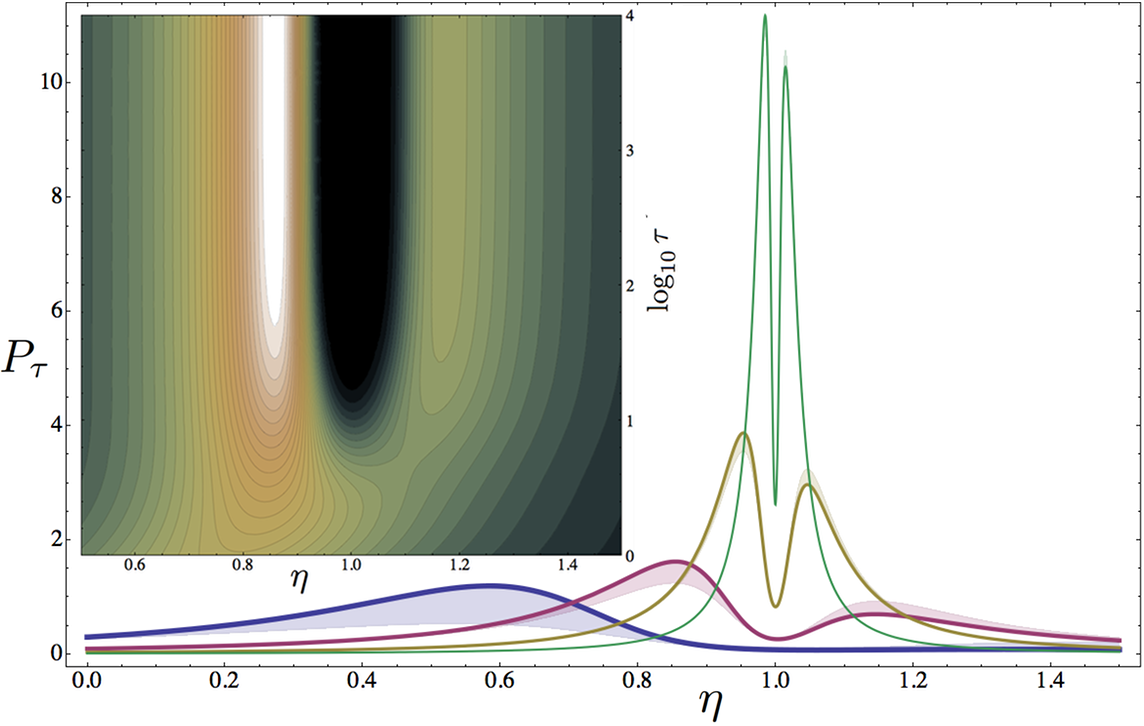
Figure 3: Main: Graphs of $(\eta,P_{\tau}(\eta))$ for $\tau=10$, $\bar{\eta}=0.3$, $\epsilon=+$ and for various coupling parameters (from bolder to thinner) $\zeta=.1,.01,.001,.0001$. The shading represents the distance to the corresponding curves for $\bar{\eta}=-1$. Inset: Contour plot of the efficiency p.d.f.’s corresponding to parameter $\zeta=0.1/\tau$ as a function of the efficiency $\eta$ and the scaled time $\tau$ (in log scale), showing that the p.d.f. is invariant at all times, hence that singular coupling stretches the relaxation times. Lighter tones for higher probabilities, darker for lower.

Nevertheless, the probabilistic level is richer. At tight coupling the bivariate Gaussian Eq. (5) becomes univariate with support along $x_{1}/x_{2}=-\varphi^{\ast}$, and the efficiency p.d.f. a Dirac delta centered at the macroscopic efficiency. Then tightly-coupled machines work macroscopically at all scaled times.

More interesting is the singular coupling. Fig. 3 shows that in this limit all extrema tend to accumulate towards the Carnot efficiency, where the density concentrates. Despite the fact that the two peaks survive, convergence to a Dirac delta can be proven by the following argument argu : From Eqs. (7,8), $h\to 1/2$, $a\to(1-\eta)^{2}$ and the efficiency p.d.f. converges to a distribution with support in $\eta=1$, which is then necessarily a finite combination of derivatives of the Dirac delta, $P_{\tau}(\eta)=\sum_{n=0}^{N}p_{n}\delta^{(n)}(1-\eta)$ hormander . Since $\langle\,g\,\rangle>0$ for all positive test functions $g(\eta)>0$, then necessarily $p_{n}=0$ but for $p_{0}=1$ $\Box$. Then, singular coupling pushes the most probable efficiency towards Carnot at fixed $\tau$; the shadings in Fig. 3 suggest that in this limit the distribution is fairly insensitive to $\bar{\eta}$. Moreover, the contour plot in Fig. 3 supports that the most probable efficiency stays at the same value for probability densities evaluated at a fixed time $\tau\propto 1/\zeta$, showing that convergence to $\bar{\eta}$ is more and more delayed. However, it must be remembered that the physical time scale is set by the entropy production rate. Necessarily the matrix entries of $L^{+}$ diverge; then in general $\bar{\sigma}$ also diverges. Still, $L^{+}$ admits a finite eigenvalue. Picking the forces along the relative eigenvector, $\phi=1+O(\zeta)$, one obtains a finite entropy production rate. Oddly, as discussed above, these conditions are met when the macroscopic machine is dud.

To resume: At singular coupling, the effect of fluctuations is macroscopically visible and permits to work close to Carnot efficiency at finite entropy production rate for sufficiently long physical times. The conditions for which the entropy production rate can be held finite are those under which the machine eventually evolves towards a dud fate. Notice that in this regime the system might flip randomly across the close sharp peaks of the p.d.f.. However, the inset in Fig. 3 suggests that at intermediate times reasonably high typical efficiencies will be favored and that a large separation between such peaks (the dark region of zero probability) occurs. Hence, to put it with a motto, a singular machine doomed to be useless might be efficiently useful for some time due to fluctuations; the better in the short run, the worse in the long. By the Green-Kubo relation Eq. (6) the singular coupling limit is approached when correlations between the currents diverge and the inverse correlation matrix becomes degenerate. It is tempting to parallel this behavior to the paradigm of criticality at phase transitions, where fluctuations become macroscopic, correlations diverge and the covariance matrix degenerates zanardi ; pole2 . In practical applications, the best figure of merit reached is $zT\approx 3$ ($\zeta=0.25$), in fact quite low. Then, we suggest that this insight might indicate a strategy to look for devices with higher figure of merit.

An important observation here to be made is that singular coupling pushes the system far from equilibrium. The framework of stochastic thermodynamics encompasses such systems by assuming that they are subtended by an underlying Markovian dynamics, giving rise to non-Gaussian current statistics. Gaussianity is only recovered in the linear regime at large times by the central limit theorem speck ; engel . While the model of a Brownian particle in a tilted plane studied in Ref. gatien1 has exact Gaussian propagators as those studied in this paper, in general Markov processes have a more complex behavior in time, in particular the average flux varies as the system evolves, depending on the initial ensemble. Then, the exact short- and large-time behavior of the efficiency distribution might become model-dependent. For asymmetric protocols, a signature of non-Gaussian behavior is the off-Carnot least-probable efficiency gatien2 ; gingrich ; roldan .

Nevertheless, our study points out that in the simplest Gaussian scenario the efficiency p.d.f. manifests peculiar features that might possibly be universal: Power-law tails, no finite moments, a naturally occurring transition to a bimodal distribution due to reverse working regimes, etc. Particularly intriguing is the limit of a degenerate or singular covariance matrix. While the former case is intrinsically macroscopic and broadly studied benenti ; entin , we obtain a clear indication that the singular coupling regime displays an interesting behavior that could lead to the enhancement of the efficiency above its macroscopic value. More light is to be shed on these issues by future inquiry on the finite-time statistics of the efficiency in stochastic models proesmans ; prost in their rich phenomenology, including maximum power generation espositomax ; schmiedl , multi-terminal machines mazza , broken time-reversal symmetry saito , the insurgence of phase transitions, and in relation to the issue of efficiency enhancement by noise hanggi or by decoherence plenio . Experimental setups that could test these predictions are already available exp1 ; exp2 ; exp3 ; exp4 ; exp5 . The full statistics of the efficiency close to equilibrium has recently been sampled for a Carnot engine realized with a Brownian particle, in the quasistatic limit where the currents’ statistics is Gaussian roldan , and data analysis farther away from equilibrium might soon be available.

Aknowledgments.

The research was supported by the National Research Fund Luxembourg in the frame of project FNR/A11/02 and of Postdoc Grant 5856127.

I Supplementary material

I.1 Efficiency p.d.f.

In this section we derive the probability density function of the efficiency. Without possibility of confusion, we will denote stochastic variables by the values they take. Let us consider two normally distributed stochastic variables $\bm{x}=(x_{1},x_{2})$ (the fluxes)

$$P_{t}(\bm{x})=\frac{t}{4\pi\sqrt{|L|}}\exp\left[-{\frac{t}{4}(\bm{x}-\bar{\bm{x}})\cdot L^{-1}(\bm{x}-\bar{\bm{x}})}\right].$$ (17)

Defining $\bm{f}=L^{-1}\bar{\bm{x}}$ (the forces), we want to calculate the p.d.f. of the efficiency

$$\eta=-\frac{f_{1}x_{1}}{f_{2}x_{2}}.$$ (18)

It is convenient to define $\sigma_{i}=f_{i}x_{i}$ (the entropy production rates) with averages $\bar{\sigma}_{i}=f_{i}\bar{x}_{i}$. Let $\bar{\sigma}=\bar{\sigma}_{1}+\bar{\sigma}_{2}$. We have

$$P^{\prime}_{t}(\sigma_{1},\sigma_{2})d\sigma_{1}d\sigma_{2}=P_{t}(x_{1},x_{2})dx_{1}dx_{2}$$ (19)

yielding

$$P^{\prime}_{t}(\sigma_{1},\sigma_{2})=\frac{t}{4\pi\bar{\sigma}\sqrt{|C|}}\exp\left[-{\frac{t}{4\bar{\sigma}}(\bm{\sigma}-\bar{\bm{\sigma}})\cdot C^{-1}(\bm{\sigma}-\bar{\bm{\sigma}})}\right].$$ (20)

Letting $L_{ij}$ be the entries of $L$, then the matrix $C$ has entries $c_{ij}=L_{ij}f_{i}f_{j}/\bar{\sigma}$ and it can be expressed as

$$C=\left(\begin{array}[]{cc}\bar{\sigma}_{1}/\bar{\sigma}-c_{12}&c_{12}\\ c_{12}&\bar{\sigma}_{2}/\bar{\sigma}-c_{12}\end{array}\right).$$ (21)

Notice that $P^{\prime}_{t}$ only depends on three parameters, $\bar{\sigma}_{1},\bar{\sigma}_{2}$ and $c_{12}$ or, equivalently, $\bar{\sigma}$, $\bar{\eta}=-\bar{\sigma}_{1}/\bar{\sigma}_{2}$ and $|C|$. Then the efficiency p.d.f. is given by

$$P_{t}(\eta) = \int d\sigma_{1}d\sigma_{2}\,\delta\left(\eta+\frac{\sigma_{1}}{\sigma_{2}}\right)P^{\prime}_{t}(\sigma_{1},\sigma_{2})$$ (22)

$$= \int d\sigma|\sigma|P^{\prime}_{t}\left(-\eta\sigma,\sigma\right).$$

We have

$$P^{\prime}_{t}(-\eta\sigma,\sigma)=\frac{t}{4\pi\bar{\sigma}\sqrt{|C|}}\exp-{\frac{t}{4\bar{\sigma}}\left[a(\eta)\sigma^{2}+2b(\eta)\sigma+c\right]}\\$$ (23)

where we introduced

$$a(\eta) = \frac{1}{|C|}(c_{22}\eta^{2}+2c_{12}\eta+c_{11})$$ (24a)

$$b(\eta) = \frac{1}{|C|}[\eta(c_{22}\bar{\sigma}_{1}-c_{12}\bar{\sigma}_{2})+c_{12}\bar{\sigma}_{1}-c_{11}\bar{\sigma}_{2}]$$ (24b)

$$c = \frac{1}{|C|}(c_{22}\bar{\sigma}_{1}^{2}-2c_{12}\bar{\sigma}_{1}\bar{\sigma}_{2}+c_{11}\bar{\sigma}_{2}^{2}).$$ (24c)

Notice that $a$ is adimensional, $b$ has dimensions of an entropy rate, and $c$ of a squared entropy rate. In fact, simple but tedious calculations show that

$$a(\eta) = (1-\eta)^{2}+\frac{1}{|C|}\left(\frac{\eta-\bar{\eta}}{1-\bar{\eta}}\right)^{2}$$ (25a)

$$b(\eta) = \bar{\sigma}(\eta-1)$$ (25b)

$$c = \bar{\sigma}^{2}\phantom{\int}.$$ (25c)

Notice that $a\geq 0$ and equality can only hold if $|L|=0$, a case that we hereby exclude. We now separate $P_{t}(\eta)=P^{+}_{t}(\eta)+P^{-}_{t}(\eta)$, where

$$P^{\pm}_{t}(\eta)=\int_{0}^{\pm\infty}d\sigma\,\sigma P^{\prime}_{t}(-\eta\sigma,\sigma).$$ (26)

Performing a change of variables $\sigma\to-\sigma$ in $P^{-}_{t}$, we have

$$P^{\pm}_{t}=\frac{t}{4\pi\bar{\sigma}\sqrt{|C|}}\int_{0}^{\pm\infty}d\sigma\,\sigma e^{-\frac{t}{4\bar{\sigma}}\left[a\sigma^{2}\pm 2b\sigma+c\right]}.$$ (27)

We can calculate the first and then change sign to $b$ to obtain the second. We obtain

$$P^{+}_{t} = \frac{1}{2\pi a\sqrt{|C|}}\int_{0}^{+\infty}d\sigma\,\frac{t(a\sigma+b-b)}{2\bar{\sigma}}e^{-\frac{t}{4\bar{\sigma}}\left(a\sigma^{2}+2b\sigma+c\right)}$$

$$= \frac{1}{2\pi a\sqrt{|C|}}\left\{\int_{0}^{+\infty}d\sigma\left[-\frac{d}{d\sigma}e^{-\frac{t}{4\bar{\sigma}}\left(a\sigma^{2}+2b\sigma+c\right)}\right]\right.$$

$$\qquad\qquad\qquad\qquad\left.-\frac{tb}{2\bar{\sigma}}\int_{0}^{+\infty}d\sigma\,e^{-\frac{t}{4\bar{\sigma}}\left(a\sigma^{2}+2b\sigma+c\right)}\right\}$$

$$= \frac{1}{2\pi a\sqrt{|C|}}e^{-\frac{tc}{4\bar{\sigma}}}\left\{1-\frac{tb}{2\bar{\sigma}}\int_{0}^{+\infty}d\sigma\,e^{-\frac{t}{4\bar{\sigma}}\left(a\sigma^{2}+2b\sigma\right)}\right\}$$

$$= \frac{1}{2\pi a\sqrt{|C|}}e^{-\frac{tc}{4\bar{\sigma}}}\left\{1-be^{\frac{tb^{2}}{4\bar{\sigma}a}}\sqrt{\frac{t}{\bar{\sigma}a}}\int_{b\sqrt{\frac{t}{4\bar{\sigma}a}}}^{+\infty}d\sigma\,e^{-\sigma^{2}}\right\}.$$

Recognizing the complementary error function $\mathrm{\,erfc}(x)=2/\sqrt{\pi}\int_{x}^{+\infty}e^{-y^{2}}dy$ and defining

$$h(\eta)=\frac{-b(\eta)}{2\bar{\sigma}\sqrt{a(\eta)}}=\frac{1-\eta}{2\sqrt{a(\eta)}}$$ (29)

we obtain

$$P^{\pm}_{t}=\frac{1}{2\pi a\sqrt{|C|}}e^{-\frac{tc}{4\bar{\sigma}}}\left\{1\pm\sqrt{\pi t\bar{\sigma}}\,h\,e^{t\bar{\sigma}h^{2}}\mathrm{\,erfc}\,(\mp\sqrt{t\bar{\sigma}}h)\right\}.$$ (30)

Introducing $\tau=t\bar{\sigma}$, the full probability distribution reads

$$P_{t}(\eta)=\frac{e^{-\frac{\tau}{4}}}{\pi a(\eta)\sqrt{|C|}}\left\{1+\sqrt{\pi\tau}\,h(\eta)\,e^{\tau h(\eta)^{2}}\mathrm{\,erf}\,\left[\sqrt{\tau}h(\eta)\right]\right\}$$ (31)

where we employed the fact that the error function $\mathrm{\,erf}=1-\mathrm{\,erfc}$ is odd.

Furthermore, defining

$$P_{t}^{++}(\eta) = \int_{\begin{subarray}{c}\sigma_{1}>0\\ \sigma_{2}>0\end{subarray}}d\sigma_{1}d\sigma_{2}\,P^{\prime}_{t}(\sigma_{1},\sigma_{2})\,\delta\left(\eta+\frac{\sigma_{1}}{\sigma_{2}}\right)$$ (32a)

$$P_{t}^{+-}(\eta) = \int_{\begin{subarray}{c}\sigma_{1}>0\\ \sigma_{2}<0\end{subarray}}d\sigma_{1}d\sigma_{2}\,P^{\prime}_{t}(\sigma_{1},\sigma_{2})\,\delta\left(\eta+\frac{\sigma_{1}}{\sigma_{2}}\right)$$ (32b)

$$P_{t}^{-+}(\eta) = \int_{\begin{subarray}{c}\sigma_{1}<0\\ \sigma_{2}>0\end{subarray}}d\sigma_{1}d\sigma_{2}\,P^{\prime}_{t}(\sigma_{1},\sigma_{2})\,\delta\left(\eta+\frac{\sigma_{1}}{\sigma_{2}}\right)$$ (32c)

$$P_{t}^{--}(\eta) = \int_{\begin{subarray}{c}\sigma_{1}<0\\ \sigma_{2}<0\end{subarray}}d\sigma_{1}d\sigma_{2}\,P^{\prime}_{t}(\sigma_{1},\sigma_{2})\,\delta\left(\eta+\frac{\sigma_{1}}{\sigma_{2}}\right)$$ (32d)

we obtain

$$P_{t}^{++}(\eta) = \theta(-\eta)P^{+}(\eta)$$ (33a)

$$P_{t}^{+-}(\eta) = \theta(+\eta)P^{-}(\eta)$$ (33b)

$$P_{t}^{-+}(\eta) = \theta(+\eta)P^{+}(\eta)$$ (33c)

$$P_{t}^{--}(\eta) = \theta(-\eta)P^{-}(\eta).$$ (33d)

I.2 Reparametrization

The task is to express $|C|$ in terms of the parameters $\zeta=|C|/c_{11}c_{22}$ and $\bar{\eta}$. Notice that $c_{11}+2c_{12}+c_{22}=1$. Then

$$\bar{\eta} = -\frac{c_{11}+c_{12}}{c_{22}+c_{12}}=-\frac{1+c_{11}-c_{22}}{1+c_{22}-c_{11}}$$ (34a)

$$\zeta = \frac{|C|}{c_{11}c_{22}}=1-\frac{(1-c_{11}-c_{22})^{2}}{4(c_{11}c_{22})}.$$ (34b)

From the first we obtain

$$c_{22}=c_{11}+\frac{1+\bar{\eta}}{1-\bar{\eta}}$$ (35)

and letting $\xi=(1+\bar{\eta})/(1-\bar{\eta})$ from the second we get

$$c_{11}^{2}+\frac{\xi\zeta-1}{\zeta}c_{11}+\frac{(\xi-1)^{2}}{4\zeta}=0$$ (36)

yielding

$$c_{11} = \frac{1-\xi\zeta}{2\zeta}\left[1\pm\sqrt{1-\zeta\left(\frac{1-\xi}{1-\xi\zeta}\right)^{2}}\right]$$ (37a)

$$= \frac{1-\xi\zeta}{2\zeta}\left(1\pm\frac{1}{1-\bar{\eta}\frac{1+\zeta}{1-\zeta}}\sqrt{\bar{\eta}^{2}-2\bar{\eta}\tfrac{1+\zeta}{1-\zeta}+1}\right)\qquad$$

$$c_{22} = \frac{1+\xi\zeta}{2\zeta}\left(1\pm\frac{1}{\frac{1+\zeta}{1-\zeta}-\bar{\eta}}\sqrt{\bar{\eta}^{2}-2\bar{\eta}\tfrac{1+\zeta}{1-\zeta}+1}\right).\qquad$$ (37b)

Given

$$1-\xi\zeta = \frac{1-\zeta}{1-\bar{\eta}}\left(1-\bar{\eta}\tfrac{1+\zeta}{1-\zeta}\right)$$ (38a)

$$1+\xi\zeta = \frac{1-\zeta}{1-\bar{\eta}}\left(\tfrac{1+\zeta}{1-\zeta}-\bar{\eta}\right)$$ (38b)

we get

$$c_{11} = \frac{1-\zeta}{2\zeta(1-\bar{\eta})}\left(1-\bar{\eta}\tfrac{1+\zeta}{1-\zeta}\pm\sqrt{\bar{\eta}^{2}-2\bar{\eta}\tfrac{1+\zeta}{1-\zeta}+1}\right)\qquad$$ (39a)

$$c_{22} = \frac{1-\zeta}{2\zeta(1-\bar{\eta})}\left(\tfrac{1+\zeta}{1-\zeta}-\bar{\eta}\pm\sqrt{\bar{\eta}^{2}-2\bar{\eta}\tfrac{1+\zeta}{1-\zeta}+1}\right).\qquad$$ (39b)

We then obtain

$$|C| = \zeta\,c_{11}c_{22}$$

$$= \frac{(1-\zeta)^{2}}{4\zeta(1-\bar{\eta})^{2}}\left(1-\bar{\eta}\tfrac{1+\zeta}{1-\zeta}\pm\sqrt{\bar{\eta}^{2}-2\bar{\eta}\tfrac{1+\zeta}{1-\zeta}+1}\right)\times$$

$$\qquad\times\left(\tfrac{1+\zeta}{1-\zeta}-\bar{\eta}\pm\sqrt{\bar{\eta}^{2}-2\bar{\eta}\tfrac{1+\zeta}{1-\zeta}+1}\right)$$

$$= -\frac{\bar{\eta}}{(1-\bar{\eta})^{2}}+\frac{1-\zeta}{2\zeta}\left(1\pm\sqrt{1-\frac{4\zeta}{1-\zeta}\frac{\bar{\eta}}{(1-\bar{\eta})^{2}}}\right).$$

I.3 Equilibrium case

We consider the case $f_{1},f_{2}\to 0$ at fixed $\varphi=f_{2}/f_{1}$. We have to evaluate Eq. (2) in the main text given that $\bm{x}=(x_{1},x_{2})$ is distributed with

$$P_{t}(\bm{x})=\frac{t}{\pi\sqrt{|L|}}\exp-{\frac{t}{4}\bm{x}\cdot L^{-1}\bm{x}}.$$ (41)

We have

$$P_{t}(-\eta\varphi x,x)=\frac{t}{\pi}\exp-{\frac{t}{4|L|}\left[a(\eta)x^{2}+2b(\eta)x+c\right]}\\$$ (42)

where we introduced

$$a(\eta)=\frac{1}{|L|}\left(L_{22}\varphi^{2}\eta^{2}+2L_{12}\varphi\eta+L_{11}\right).$$ (43)

All follows as for the derivation of the general efficiency p.d.f., but for $b=c=h=0$. Then the p.d.f. reads

$$P_{t}(\eta)=\frac{2\varphi}{\pi a(\eta)\sqrt{|L|}}.$$ (44)

I.4 Degenerate case (Tight coupling)

Let $|L|=0$. Under our conditions $L_{12}\leq 0$, we have

$$L_{12}=-\sqrt{L_{11}L_{22}}.$$ (45)

The eigenvectors of $L$ are: $(\sqrt{L_{11}},-\sqrt{L_{22}})^{T}$ relative to eigenvalue $L_{11}+L_{22}=\mathrm{\,tr}\,L$, and $(\sqrt{L_{22}},\sqrt{L_{11}})^{T}$ relative to eigenvalue $0$. Let

$$U=\frac{1}{\sqrt{L_{11}+L_{22}}}\left(\begin{array}[]{cc}\sqrt{L_{11}}&\sqrt{L_{22}}\\ -\sqrt{L_{22}}&\sqrt{L_{11}}\end{array}\right)$$ (46)

be the orthogonal matrix that performs the change of coordinate into the diagonal matrix $\Delta=\mathrm{\,diag}\,\{L_{11}+L_{22},0\}$. Then

$$\sqrt{L}=U\,\sqrt{\Delta}\,U^{T}=\frac{L}{\sqrt{L_{11}+L_{22}}}.$$ (47)

Furthermore, we introduce the Moore-Penrose pseudoinverse of $L$ which is obtained by inverting all nonvanishing eigenvalues:

$$L^{+}=U\,\left(\begin{array}[]{cc}(L_{11}+L_{22})^{-1}&0\\ 0&0\end{array}\right)\,U^{T}=\frac{L}{(L_{11}+L_{22})^{2}}$$ (48)

Letting $\Delta\bm{x}=(\bm{x}-\bar{\bm{x}})$, it is known that a degenerate normal distribution is supported along the direction

$$\Delta\bm{x}=\sqrt{L}\,\bm{y}=\sqrt{\frac{L_{11}y_{1}-L_{22}y_{2}}{L_{11}+L_{22}}}\left(\begin{array}[]{c}\sqrt{L_{11}}\\ -\sqrt{L_{22}}\end{array}\right),\quad\bm{y}\in\mathbb{R}^{2}$$ (49)

and that it has probability density

$$P_{t}(\bm{x})=\delta\left(\Delta x_{2}+\sqrt{\frac{L_{22}}{L_{11}}}\,\Delta x_{1}\right)\sqrt{\frac{t}{4\pi L_{11}}}e^{-\frac{t}{4}\Delta\bm{x}\cdot L^{+}\Delta\bm{x}}.$$ (50)

Moreover, the average currents are not arbitrary but we have $\bar{\bm{x}}=L\bm{f}$, which implies

$$P_{t}(\bm{x})=\delta\left(x_{2}+\sqrt{\frac{L_{22}}{L_{11}}}\,x_{1}\right)\sqrt{\frac{t}{4\pi L_{11}}}e^{-\frac{t}{4}\Delta\bm{x}\cdot L^{+}\Delta\bm{x}}.$$ (51)

Then, using a test function $g(\eta)$, we have

$$\langle\,g\,\rangle_{t} = \int d\eta\,g(\eta)\int dx_{1}dx_{2}\,\delta\left(\eta+\frac{x_{1}f_{1}}{x_{2}f_{2}}\right)P_{t}(x_{1},x_{2})$$ (52)

$$= \int dx_{1}dx_{2}\,g\left(-\frac{x_{1}}{x_{2}\varphi}\right)\delta\left(x_{2}+\sqrt{\frac{L_{22}}{L_{11}}}\,x_{1}\right)\times$$

$$\qquad\times\,\sqrt{\frac{t}{4\pi L_{11}}}\,e^{-\frac{t}{4}\Delta\bm{x}\cdot L^{+}\Delta\bm{x}}$$

$$= g\left(\varphi^{\ast}/\varphi\right).$$

By Eq. (16) in the main text at $\zeta\to 0$, $\varphi^{\ast}/\varphi\to\bar{\eta}$.

I.5 Fluctuation relation for self-dual p.d.f.

The two maxima of $P_{\tau}(\eta)$ are due to converse regimes. It is then natural to define the stochastic variable $\eta^{\ast}=-\sigma_{2}/\sigma_{1}$ and look at its p.d.f.

$$P^{\ast}_{\tau}(\eta)=\eta^{-2}P_{\tau}(1/\eta)$$ (53)

Self-duality is the condition upon which $P^{\ast}_{\tau}(\eta)=P_{\tau}(\eta)$, implying the following fluctuation relation for the efficiency

$$P^{\mathrm{\,s.d.}}_{\tau}(\eta)=\frac{1}{\eta^{2}}\,P^{\mathrm{\,s.d.}}_{\tau}(1/\eta)$$ (54)

Let us show that the choice $\varphi=\varphi^{\ast}$ yields this fluctuation relation. First, it simple to show that $\varphi=\varphi^{\ast}=\sqrt{L_{11}/L_{22}}$ implies the symmetry of the normal multivariate for the currents

$$P^{\mathrm{\,\mathrm{s.d.}}}_{t}(x_{1},x_{2})=P^{\mathrm{\,\mathrm{s.d.}}}_{t}\left(\varphi x_{2},{\varphi}^{-1}x_{1}\right).$$ (55)

In fact, the Jacobian of the transformation $(x_{1},x_{2})\to(\varphi x_{2},\varphi^{-1}x_{1})$ is $1$, and the identity between the quadratic polynomials at exponent can be checked by direct substitution:

$$L_{22}(x_{1}-\bar{x}_{1})^{2}-2L_{12}(x_{1}-\bar{x}_{1})(x_{2}-\bar{x}_{2})+L_{11}(x_{2}-\bar{x}_{2})^{2}=\\ =L_{22}(\varphi x_{2}-\bar{x}_{1})^{2}-2L_{12}(\varphi x_{2}-\bar{x}_{1})(x_{1}/\varphi-\bar{x}_{2})+L_{11}(x_{1}/\varphi-\bar{x}_{1})^{2}$$ (56)

In fact, equating order by order one can also show that the choice $\varphi=\pm\varphi^{\ast}$ are the only ones yielding Eq. (55).

Now let us consider the efficiency p.d.f.:

$$P^{\mathrm{\,s.d.}}_{t}(\eta) = \varphi\int dx|x|P^{\mathrm{\,s.d.}}_{t}\left(-\eta\varphi x,x\right)$$

$$= \varphi\int dx|x|P^{\mathrm{\,s.d.}}_{t}\left(\varphi x,-\eta x\right)$$

$$= \frac{\varphi}{|\eta|\eta}\int_{y(-\infty)}^{y(+\infty)}dy|y|P^{\mathrm{\,s.d.}}_{t}\left(-\varphi y/\eta,y\right)$$

$$= \frac{\varphi}{\eta^{2}}\int dy|y|P^{\mathrm{\,s.d.}}_{t}\left(-\varphi y/\eta,y\right)~{}=~{}\frac{1}{\eta^{2}}P^{s.d.}_{t}(1/\eta)$$

where on the third line we performed the change of coordinates $y(x)=-\eta x$ and we kept into account the order of the extremes of integration by including a suitable absolute value.

I.6 Efficiency at singular coupling

We say the covariance matrix tends to become singular when its inverse tends to become degenerate. Let $\varepsilon(\zeta)$ be small of order $\zeta$. An almost degenerate inverse takes the form

$$L^{-1}=\left(\begin{array}[]{cc}m_{11}&(1-\varepsilon)\sqrt{m_{11}m_{22}}\\ (1-\varepsilon)\sqrt{m_{11}m_{22}}&m_{22}\end{array}\right).$$ (60)

Then we have

$$L=\frac{1}{2\varepsilon}\left(\begin{array}[]{cc}L_{11}&(\varepsilon-1)\sqrt{L_{11}L_{22}}\\ (\varepsilon-1)\sqrt{L_{11}L_{22}}&L_{22}\end{array}\right)$$ (63)

where $L_{11}=m_{11}^{-1}$, $L_{22}=m_{22}^{-1}$. Eigenvalues:

$$\lambda_{+} = \frac{1}{2\epsilon}(L_{11}+L_{22})\left(1-2\varepsilon\frac{L_{1}L_{2}}{(L_{11}+L_{22})^{2}}\right)$$ (64a)

$$\lambda_{-} = \frac{L_{1}L_{2}}{L_{11}+L_{22}}.$$ (64b)

The first is divergent, the second finite. The eigenvector $\bm{f}_{-}$ relative to the finite eigenvalue is such that

$$\frac{f_{1}}{f_{2}}=\sqrt{\frac{L_{22}}{L_{11}}}\left(1+\varepsilon\frac{L_{11}-L_{22}}{L_{11}+L_{22}}\right).$$ (65)

Therefore

$$\phi=\varphi/\varphi^{\ast}=\left(1+\varepsilon\frac{L_{22}-L_{11}}{L_{11}+L_{22}}\right).$$ (66)

By Eq. (16) the macroscopic efficiency along this eigenvectors reads

$$\bar{\eta}=-1+O(\zeta^{2}).$$ (67)

I.7 Critical time

The critical time is defined as the scaled time at which an inflection point appears in the p.d.f. of the efficiency. Fig. 4 provides a color plot of the critical time.

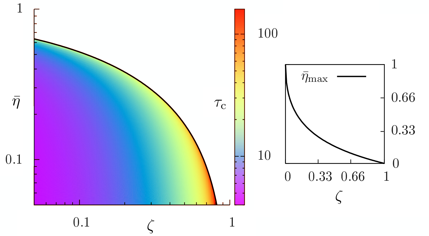
Figure 4: Color plot of $\tau_{\mathrm{c}}$ as a function of the tight coupling parameter $\zeta$ and of the macroscopic efficiency $\bar{\eta}$, for $\epsilon=+$, in log-log scale. Inset: maximal efficiency as a function of the coupling parameter, in natural scale.

References

(1) G. Verley, T. Willaert, C. Van den Broeck and M. Esposito, Nat. Commun. 5, 4721 (2014).
(2) G. Verley, T. Willaert, C. Van den Broeck and M. Esposito, Phys. Rev. E 90, 052145 (2014).
(3) T. R. Gingrich, G. M. Rotskoff, S. Vaikuntanathan, P. L. Geissler, New J. Phys. 16, 102003 (2014).
(4) H. Touchette, Phys. Rep. 478, 1, (2009).
(5)I. A. Martinez, E. Roldan, L. Dinis, D. Petrov, J. M. R. Parrondo, R. Rica, arXiv:1412.1282.
(6) S. Rana, P. S. Pal, A. Saha and A. M. Jayannavar, Phys. Rev. E 90, 042146 (2014).
(7) S. R. De Groot and P. Mazur, Non-equilibrium thermodynamics (Courier Dover Publications, New York, 2013).
(8) U. Seifert, Rep. Progr. Phys. 75, 126001 (2012).
(9) C. Van den Broeck and M. Esposito, Physica A 418, 6 (2015).
(10) G. N. Bochkov and Y. E. Kuzovlev, Physica A 106, 443 (1981); ibid. 480 (1981).
(11) M. Polettini and M. Esposito, J. Stat. Mech. P10033 (2014).
(12) D. Andrieux and P. Gaspard, J. Chem. Phys. 121, 6167 (2004).
(13) G. Benenti, K. Saito and G. Casati, Phys. Rev. Lett. 106, 230602 (2011).
(14) K. Proesmans, B. Cleuren, C. Van Den Broeck, arXiv:1411.3531.
(15) M. Abramowitz and I. A. Stegun, Handbook of Mathematical Functions with Formulas, Graphs, and Mathematical Tables (Dover, New York, 1965).
(16) O. Entin-Wohlman, J.-H. Jiang and Y. Imry, Phys. Rev. E 89, 012123 (2014).
(17) Discussion with user Kostya_I on mathoverflow.net, http://mathoverflow.net/questions/178859/
power-law-distribution-with-support-in-x-0
(18) L. Hörmander, The analysis of linear partial differential operators I (Springer, Berlin, 1983).
(19) P. Zanardi, P. Giorda and M. Cozzini, Phys. Rev. Lett. 99, 100603 (2007);
(20)M. Polettini, Eur. Phys. J. B 87, 215 (2014).
(21) T. Speck and U. Seifert, Phys. Rev. E 70, 066112 (2004).
(22) J. Hoppenau, and A. Engel, J. Stat. Mech. 06, P06004 (2013).
(23)F. Jülicher, A. Ajdar and J. Prost, Rev. Mod. Phys. 69, 1269 (1997).
(24) M. Esposito, K. Lindenberg and C. Van den Broeck, Phys. Rev. Lett. 102, 130602 (2009).
(25) T. Schmiedl and U. Seifert, Eur. Phys. Lett. 81, 20003 (2008).
(26)F. Mazza, R. Bosisio, G. Benenti, V. Giovannetti, R. Fazio and F. Taddei, New J. Phys. 16, 085001 (2014).
(27) K. Saito, G. Benenti, G. Casati, and T. Prosen, Phys. Rev. B 84, 201306 (2011).
(28) J. Spiechowicz, P. Han̈ggi, J.Łuczka, Phys. Rev. E 90, 032104 (2014).
(29) F. Caruso, A. W. Chin, A. Datta, S. F. Huelga and M. B. Plenio, J. Chem. Phys. 131, 105106 (2009).
(30) D. Collin, F. Ritort, C. Jarzynski, S. B. Smith, I. Tinoco and C. Bustamante, Nature 437 231-234 (2005).
(31) A. Bérut, A. Arakelyan, A. Petrosyan, S. Ciliberto, R. Dillenschneider, and E. Lutz, Nature, 483, 187-189 (2012).
(32) J. V. Koski, T. Sagawa, O-P. Saira, Y. Yoon, A. Kutvonen, P. Solinas, M. Möttönen, T. Ala-Nissila and J. P. Pekola, Nature Phys. Lett. 9, 644
(2013).
(33) S. Ciliberto, A. Imparato, A. Naert and M. Tanase, Phys. Rev. Lett. 110, 180601 (2013).
(34) C. Tietz, S. Schuler, T. Speck, U. Seifert and J. Wrachtrup, Phys. Rev. Lett. 97, 050602 (2006).
(35) See the Supplementary Material for details regarding the derivation of the efficiency PDF, the parametrization, and the various limiting situations.