Differential analysis of nonlinear systems:
revisiting the pendulum example

Abstract

Differential analysis aims at inferring global properties of nonlinear behaviors from the local analysis of the linearized dynamics. The paper motivates and illustrates the use of differential analysis on the nonlinear pendulum model, an archetype example of nonlinear behavior. Special emphasis is put on recent work by the authors in this area, which includes a differential Lyapunov framework for contraction analysis [24], and the concept of differential positivity [25].

I Introduction

The purpose of this tutorial paper is to revisit the role of linearization in nonlinear systems analysis and to present recent developments of this differential approach to systems and control theory. Linearization is often considered as a synonym of local analysis, whereas nonlinear systems analysis aims at a global understanding of the system behavior. The focus of the paper is therefore on system properties that allow to address non-local questions through the local-in-nature analysis of a differential approach. Such properties have been sporadically studied in the control community, perhaps most importantly through the contraction property advocated in the seminal paper of Lohmiller and Slotine [40], but they play at best a secondary role in the main textbooks of nonlinear control. While it is not the aim of the present tutorial to provide a comprehensive survey of the role of differential analysis in systems and control (a partial account of which can be found in Section VI of [24]; see also the other paper of this tutorial session [2]), we will illustrate some questions that have stimulated a renewed interest for differential analysis in the recent years. The interested reader is also referred to the two-part invited session of CDC2013 for a sample of recent developments in that area.

Owing to the tutorial nature of the paper, the discussion will be exclusively restricted to the classical (adimensional) nonlinear pendulum model

$$\Sigma:\left\{\begin{array}[]{rcl}\dot{\vartheta}&=&v\\ \dot{v}&=&-\sin(\vartheta)-kv+u\end{array}\right.\quad(\vartheta,v)\in\mathcal{X}:=\mathbb{S}\times{\mathbb{R}}\ ,$$ (1)

where $k\geq 0$ is the damping coefficient and $u$ is the torque input. The specific aim of the paper is therefore to understand as much as possible of the global behavior of model (1) from its linearized dynamics ($(\delta\vartheta,\delta v)\in T_{(\vartheta,v)}\mathcal{X}$)

$$\left[\begin{array}[]{c}\dot{\delta\vartheta}\\ \dot{\delta v}\end{array}\right]=\underbrace{\left[\begin{array}[]{cc}0&1\\ -\cos(\vartheta)&-k\end{array}\right]}_{=:A(\vartheta,k)}\left[\begin{array}[]{c}\delta\vartheta\\ \delta v\end{array}\right]+\left[\begin{array}[]{c}0\\ \delta u\end{array}\right]$$ (2)

where any solution $(\delta\vartheta(\cdot),\delta v(\cdot))$ lives at each time instant $t$ in the tangent space $T_{(\vartheta(t),v(t))}\mathcal{X}$, where $(\vartheta(\cdot),v(\cdot))$ is a solution to (1).

The nonlinear pendulum model is an archetype example of nonlinear systems analysis. As a control system, it is one of the simplest examples of nonlinear mechanical models and many of its properties extend to more complex electro-mechanical models such as models of robots, spacecrafts, or electrical motors. As a dynamical system, it is one the simplest models to exhibit a rich and possibly complex global behavior, owing to the interplay between small oscillations and large oscillations, two markedly distinct behaviors for which everyone has a clear intuition developed since childhood.

At the onset, it is worth observing that the pendulum is a nonlinear model for two related but distinct reasons: the vector field is nonlinear due to the sinusoidal nature of the gravity torque but also the state-space is nonlinear due to the angular nature of the pendulum position. In fact it could be argued that the nonlinearity of the space is more fundamental than the nonlinearity of the vector field in that example, and this feature of the pendulum extends to most nonlinear models encountered in engineering. The differential analysis, which linearizes both the space and the vector field, is perhaps especially relevant for such models.

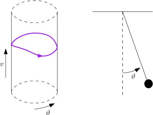
Figure 1: The natural state-space of the pendulum (left). The measure of the angle $\vartheta$ (right).

The paper is organized as follows. Section II revisits the pendulum example from a classical nonlinear control perspective, pointing to some limitations of nonlinear control that call for a differential viewpoint. Section III revisits the pendulum example from a dynamical system perspective, summarizing the main geometric properties of its limit sets. Section IV introduces the differential analysis, starting with the classical role of linearization in the local analysis of hyperbolic limit sets, and gradually moving to the differential Lyapunov framework recently advocated by the authors [24]. The section concludes on a short discussion on horizontal contraction, a property that purposely excludes specific directions in the tangent space from the contraction analysis. Section V illustrates on the pendulum example the novel concept of differential positivity [25], which is a projective form of differential contraction owing to the positivity of the linearized dynamics. We will illustrate how differential positivity provides a novel tool for the differential analysis of limit cycles and, more generally, of one-dimensional attractors.

II A nonlinear control perspective

II-A Feedback linearization and incremental dynamics

The pendulum is feedback linearizable: the control input

$$u=\sin(\vartheta)+w$$ (3)

transforms the nonlinear pendulum model into the linear system

$$\begin{array}[]{rcl}\dot{\vartheta}&=&v\\ \dot{v}&=&-kv+w\ .\end{array}$$ (4)

Achieving linearity by feedback has been a cornerstone of nonlinear control theory and is a key property for a regulation theory of nonlinear systems [33].

Exploiting linearity, it is straightforward to see that solving tracking or regulation problems on (4) become trivial tasks in comparison to the fully nonlinear case. The combination of the nonlinear cancellation in (3) with a linear stabilizing feedback and a feedforward injection would guarantee the asymptotic tracking of any suitable reference trajectory in $(\vartheta^{*}(\cdot),v^{*}(\cdot))\in{\mathbb{R}}\to\mathcal{X}$.

A key difference between the nonlinear pendulum dynamics and the linear dynamics (4) is in the incremental property: if $(\vartheta_{1}(\cdot),v_{1}(\cdot))$ and $(\vartheta_{2}(\cdot),v_{2}(\cdot))$ are two solutions of (1) for two different inputs $u_{1}(\cdot)$ and $u_{2}(\cdot)$, the increment $(\Delta\vartheta(\cdot),\Delta v(\cdot))=(\vartheta_{1}(\cdot)-\vartheta_{2}(\cdot),v_{1}(\cdot)-v_{2}(\cdot))$ satisfies

$$\Delta\Sigma:\left\{\begin{array}[]{rcl}\dot{\Delta\vartheta}&=&\Delta v\\ \dot{\Delta v}&=&-(\sin(\vartheta_{1})-\sin(\vartheta_{2}))-k\Delta v+\Delta u\end{array}\right.$$ (5)

whose right-hand side differs from the original one. Even the definition of the angular error $\Delta\vartheta$ calls for some caution because of the nonlinear nature of angular variables.

The basic observation that the dynamics and incremental dynamics are equivalent only for linear systems is a fundamental bottleneck of nonlinear systems theory. Regulation, tracking, and observer design all involve the stabilization of the incremental dynamics. Only in linear system theory is the error between two arbitrary solutions equivalent to the error between one solution and the zero equilibrium solution.

Feedback linearization makes the dynamics and the incremental dynamics equivalent. But if the compensation of nonlinear terms by feedback is not possible, regulation theory becomes challenging even for the nonlinear pendulum, and requires incremental stability properties. This is a main motivation for contraction theory, which seeks to exploit the stability properties of the linearized dynamics, that is, the incremental dynamics for infinitesimal differences, in order to infer incremental stability properties.

II-B Energy-based Lyapunov control

Inherited from classical methods from physics, methods based on the conservation/dissipation of energy are central in nonlinear control. The undamped pendulum preserves the sum of kinetic and potential energy

$$E:=\frac{v^{2}}{2}+\cos(\vartheta)$$ (6)

during its motion, while it dissipates energy when the damping is nonzero $k>0$. For open systems, dissipativity theory relates the energy dissipation to an external power supply [68, 69]: the energy is an internal storage that satisfies the balance

$$\dot{E}\leq u\dot{\vartheta}$$ (7)

meaning that its rate of growth cannot exceed the mechanical power supplied to the system. Using $y:=\dot{\vartheta}$ to denote the output of the system, dissipativity with the supply $uy$ is a passivity property. Passivity is closely related to Lyapunov stability. The static output feedback $u=-y$ adds damping in the system and is often sufficient to achieve asymptotic stability of the minimum energy equilibrium. For open systems, the supply rate measures the effect of exogenous signals on the internal energy of the system.

Passivity based control is a building block of nonlinear control theory and has led to far reaching generalizations in the theory of port-Hamiltonian systems [65, 46], leading to an interconnection theory for the energy-based stabilization of electro-mechanical systems. For instance, the fundamental interconnection property that the feedback interconnection of passive systems provides a direct solution to the PI control of passive systems because a PI controller is a passive system.

But a bottleneck of passivity theory is the generalization from stabilization to tracking control. Fundamentally, this is because the dissipativity relationship seems of no direct use to analyze the stability properties of the incremental dynamics. The energy – or the storage – provides a natural distance between an arbitrary state and the state of minimum energy but it does not provide a natural distance between two arbitrary solutions.

II-C Lure systems and Kalman conjecture

Figure 2 illustrates that the nonlinear pendulum is a Lure system, that is, it admits the feedback representation of a linear system with a static nonlinearity. The analysis of Lure systems is another building block of nonlinear system theory, allowing to exploit the frequency-domain properties of the linear system in the stability analysis of the nonlinear system.

Figure 2: The representation of the pendulum in ${\mathbb{R}}^{2}$ as the negative feedback loop of a linear system with a sector nonlinearity.

Absolute stability theory seeks to characterize sufficient conditions of the static nonlinearity to guarantee stability of the feedback system. Most conditions for absolute stability would not apply to the pendulum because they consider a static nonlinearity in a linear space, whereas the sinusoidal nonlinearity should be considered as a static map defined on the circle.

But one relevant exception is the work of Kalman, which formulates conditions on the linearization of the nonlinearity. For a static nonlinearity satisfying the condition $a\leq\sigma^{\prime}(y)\leq b$, Kalman conjectured stability of the nonlinear system if the feedback system is stable for any constant gain $k\in[a,b]$, [35].

Kalman’s conjecture is a particular case of the Markus-Yamabe conjecture [42, 16], which infers global asymptotic stability properties for the nonlinear system $\dot{x}=f(x)$ from stability of the “pointwise” linearization $\dot{\delta x}=\partial f(x)\delta x$ at any point $x$. A counter-example to Kalman conjecture eventually disproved both conjectures [27] but the attempt is a typical example of differential analysis: global properties of the nonlinear system are inferred from local analysis of the infinitesimal properties.

III A dynamical systems perspective

III-A Limits sets and bifurcations

For a fixed constant torque input, the pendulum model is a two-dimensional system that can be studied using phase portrait techniques, allowing for a complete characterization of its limit sets.

Figure 3 from [64, Section 8.5] summarizes the possible asymptotic behaviors of the model as a function of two parameters: the damping coefficient $k$ and the constant level of the torque $u$. For large values of the damping, a constant input torque $|u|\leq 1$ forces the trajectories to converge to a fixed point: either the stable downward equilibrium, or the unstable upward equilibrium for solutions initialized on the one-dimensional stable manifold of this saddle point. For a torque magnitude $|u|>1$, the unique limit set is a globally attractive limit cycle. For small damping $k$, solutions still converge either to a fixed point for small torque or to a limit cycle for large torque, but an intermediate region exists in the parameter space where the stable limit cycle behavior coexists with the stable fixed point. This bistable behavior exists if the damping parameter does not exceed a critical damping $k_{c}$. The overall behavior is summarized in Figure 3.

Figure 3: The qualitative behavior of the pendulum for large/small values of torque and damping, as reported in [64]

Specific bifurcations delineate the different types of asymptotic behavior in the parameter space. For large damping, the two fixed points existing for $u<1$ approach each other as the torque is increased to eventually merge in a single fixed point for $u=1$ in a so-called infinite-period bifurcation [64, Section 8.4].

A different bifurcation scenario gives rise to the bistable region in Figure 3. For any $k<k_{c}$ there exists a critical value $u=u_{c}(k)$ for which the pendulum encounters a homoclinic bifurcation. (see [64, Section 8.5] and Figures 8.4.3, 8.5.7 and 8.5.8 therein). For decreasing value of $u_{c}(k)<u<1$ the limit cycle gets closer to the unstable manifold of the saddle. At $u=u_{c}(k)$ the limit cycle merges with the unstable manifold of the saddle, which also coincides with the stable manifold of the saddle (see Figure 4), and disappear for $u<u_{c}(k)$. For $u_{c}(k)<u<1$, the stable manifold of the saddle is an important geometric object: it separates the basin of attraction of the stable fixed point from the basin of attraction of the limit cycle.

Figure 4: A homoclinic horbit connects the unstable manifold of the saddle with its stable manifold. The saddle point is the $\alpha$ and $\omega$ limit set of each point within the homoclinic orbit.

III-B The overdamped pendulum

For large damping, further insight on the qualitative dynamics is provided by singular perturbation analysis, which exploits the analysis of the singular behavior obtained in the limit of infinitely separated time-scales.

Time scale separation on the pendulum is dictated by the damping coefficient. In the overdamped limit, the two-dimensional behavior decouples into two one-dimensional behaviors, which is a drastic simplification. Following [64, Section 4.4], in the overdamped limit $k\to\infty$, the pendulum dynamics reduces to a first order (open gradient) dynamics represented by the (normalized) equation

$$\dot{\vartheta}=-\sin(\vartheta)+u\ .$$ (8)

For instance, in the overdamped limit the velocity component of (1) reads $kv=-\sin(\vartheta)+u$. Thus, $k\dot{\vartheta}=-\sin(\vartheta)+u$ which, by time reparameterization $k\tau=t$, gives (8).

The one-dimensional model (8) captures the qualitative behavior of the pendulum for large damping: it has two fixed points for $|u|<1$ and no fixed points, meaning a periodic behavior, for $|u|>1$. The saddle-node bifurcation at $u=1$ is the one-dimensional analog of the infinite period bifurcation of the two-dimensional pendulum. In contrast, the bistable behavior of the pendulum for smaller damping is not captured under the time-scale separation assumption.

III-C Ingredients for complex attractors

The nonlinear pendulum is especially valuable as a prototype example of dynamical systems textbooks in that it illustrates a fundamental route to hyperbolic strange attractors: the simple bistable behavior reviewed in the previous section for small damping can be turned into a complex chaotic behavior under a weak harmonic input of the type $u=\epsilon\sin(\omega t)$.

This is because the saddle homoclinic orbit that exists in the range of small damping and small torque: it allows for recurrence of the saddle point neighborhood, that is, trajectories that start close to the saddle point can return to the saddle point after a large excursion, together with sensitivity of the initial condition: a small perturbation near the saddle point can change the small or large oscillation fate of the trajectory. Such behavior is the essence of Smale’s construction of hyperbolic strange attractors [60, pp. 843-852] and the stable manifold theorem.

In that sense, the homoclinic orbit illustrated in Figure 4 is a fundamental ingredient of complex behaviors. And it has a particularly simple and concrete interpretation in the nonlinear pendulum model as the geometric object that separates small oscillations from large oscillations for small damping and small torque. The next sections will illustrate how this global property can be captured in a differential framework.

IV A differential perspective

IV-A Linearization and local analysis

Differential methods recognize that the analysis of the linearization of the system dynamics along trajectories captures important properties of the system behavior. They are the essence of local stability analysis. The simplest case is provided by Lyapunov’s first method, for the analysis of the local stability properties of fixed points. For the pendulum with zero torque, the linearization of the dynamics is given by (2) and $\delta u=0$. The eigenvalues of the state matrix

$$A(\vartheta,k)=\left[\begin{array}[]{cc}0&1\\ -\cos(\vartheta)&-k\end{array}\right]$$ (9)

at the fixed points $(\vartheta,v)\in\{(0,0),(\pi,0)\}$ reveal that the fixed point in zero is locally asymptotically stable, while the other fixed point is a saddle.

Lyapunov’s first method rests on the observation that any trajectory $(\delta\vartheta(\cdot),\delta v(\cdot))$ of (2) at the fixed point $(\vartheta,v)=(0,0)$ is an approximation of the infinitesimal mismatch between the trajectory $(\vartheta(t),v(t))=(0,0)$ at equilibrium and the trajectory $(\hat{\vartheta}(\cdot),\hat{v}(\cdot))$ arising from an infinitesimal initial variation given by $\hat{\vartheta}(t_{0})-\vartheta(t_{0})=\delta\vartheta(t_{0})$ and $\hat{v}(t_{0})-v(t_{0})=\delta v(t_{0})$. Indeed, exponential stability of the linearization implies asymptotic convergence of $(\hat{\vartheta}(\cdot),\hat{v}(\cdot))$ to the fixed point. In that sense, the linearization captures the infinitesimal incremental dynamics in the neighborhood of a particular solution.

A similar approach captures the local stability properties of limit cycles. Let $(\vartheta(\cdot),v(\cdot))$ be the periodic trajectory of the pendulum for some $u>1$. Periodicity reads: there exists a time interval $T>0$ such that $(\vartheta(t+T),v(t+T))=(\vartheta(t),v(t))$ for all $t$. The fundamental matrix solution $\Phi(\cdot)$ of the linearization (2) along the periodic trajectory $(\vartheta(\cdot),v(\cdot))$ satisfies

$$\dot{\Phi}(t)=A(\vartheta(t),k)\Phi(t)$$ (10)

that, by periodicity, leads to the identity $\Phi(t+T)=\Phi(t)$  . Considering the initial condition $\Phi(0)=I$ ($I$ is the identity matrix), the eigenvalues $\rho_{1},\dots,\rho_{n}$ of the update map

$$\Delta_{T}:=\Phi(T)$$ (11)

are the characteristic Floquet multipliers of the periodic trajectory $(\vartheta(\cdot),v(\cdot))$. These eigenvalues characterize the behavior of the nonlinear pendulum in the neighborhood of the periodic trajectory [28, Section 1.5].

Looking at Figure 5, in an infinitesimal neighborhood of the periodic trajectory, the update map captures the convergence among neighboring trajectories crossing the Poincaré section transversal to the system flows. Indeed, $n-1$ Floquet multipliers smaller than one imply local asymptotic stability of the limit cycle (by symmetry, one multiplier is necessarily equal to one).

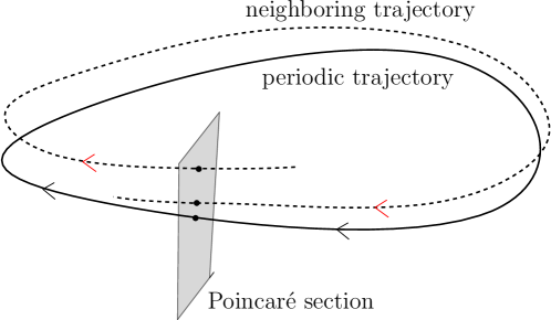
Figure 5: $n-1$ Floquet multipliers smaller than one guarantees contraction of the Poincaré map, thus local attractiveness of the limit cycle.

The study of the linearized dynamics plays a fundamental role also in the characterization of chaotic behaviors, through the notion of Lyapunov exponents, [11, 67]. The maximal Lyapunov exponent is a measure of the maximal separation rate between two infinitesimally close trajectories, which makes contact with the sensitivity of trajectories with respect to initial conditions. The maximal Lyapunov exponent is captured by the growth rate of the fundamental solution, which for the pendulum reads

$$\lim_{t\to\infty}\frac{1}{t}\ln|\Phi(t)|$$ (12)

computed along any system trajectory $(\vartheta(\cdot),v(\cdot))$ from the initial condition $\Phi(0)=I$. Clearly, the maximal Lyapunov exponent depends on the particular trajectory $(\vartheta(\cdot),v(\cdot))$ along which the linearization is computed. The limit in (12) clarifies, however, that such a dependence is related to the particular attractor to which the trajectory converge. The selection of a particular matrix norm may change the value of the maximal Lyapunov exponent. For systems with bounded trajectories, a positive maximal Lyapunov exponent is an indicator of possible chaotic behaviors.

IV-B From Kalman’s conjecture to differential Lyapunov theory

The aim of differential analysis is to exploit the properties of the linearized dynamics beyond the local stability analysis of attractors. Kalman’s conjecture and Markus-Yamabe conjecture illustrate attempts to infer global properties of the nonlinear system from the analysis of linearized dynamics.

The conditions of the Kalman’s conjecture are based on the linearized dynamics of a Lure system $\dot{x}=f(x):=Ax-B\sigma(Cx)$ where $(A,B,C)$ is a minimal state-space representation of the linear system in feedback interconnection with the static nonlinearity $\sigma(\cdot)$. Requiring that the matrix $(A-\mu BC)$ is Hurwitz for any $\mu$ is equivalent to check that the Jacobian matrix $\partial f(x)$ is Hurwitz for any $x$, showing that Kalman’s conjecture is a particular case of the Markus-Yamabe conjecture [35, 42, 16]. It is well known that a Huwitz Jacobian matrix does not guarantee stability [38, Perron Effects], [37]. In fact, within the reformulation based on the Jacobian, Kalman’s condition reads

$$\partial f(x)^{T}P(x)+P(x)\partial f(x)<0\qquad\forall x\ ,$$ (13)

where $P(x)$ is a positive and symmetric matrix for each $x$. However, the variation of $P(x)$ cannot be neglected, which requires the satisfaction of the extended condition

$$\partial f(x)^{T}P(x)+P(x)\partial f(x)+\dot{P}(x)<0\qquad\forall x\ ,$$ (14)

where $\dot{P}(x)$ represents the variation of the “metric” along the vector field $f(x)$.

The gap between the Jacobian conjecture and a sufficient condition for global asymptotic stability thus relates to analyzing the stability properties of the frozen linearized dynamics at every point instead of along a specific trajectory.

The “stability” condition (14) allows for an interesting geometric reinterpretation when the matrix $P(x)$ is the representation, in coordinates, of a Riemannian tensor. (14) provides a coordinate formulation of the contraction of the Riemannian tensor along the flow of the system. As a consequence, given a positive and symmetric matrix $P(x)$, smooth in $x$, condition (14) guarantees not only that the fixed point of the nonlinear dynamics is asymptotically stable, but also that the nonlinear dynamics is contractive, that is, any pair of solutions $x(\cdot),z(\cdot)$ of the differential equation $\dot{x}=f(x)$ satisfy

$$\lim_{t\to\infty}d(x(t),z(t))=0\ ,$$ (15)

where $d$ is the Riemannian distance provided by the Riemannian tensor by integration along geodesics. Interestingly, if the induced distance and the state space of the system define a complete metric space, the existence of a stable fixed point follows from the contraction mapping theorem. This is the essence of the contraction analysis advocated by Lohmiller and Slotine, [40].

The key observation is that the asymptotic stability of the linearized dynamics guarantees that the nonlinear system is contractive. It follows that the nonlinear dynamics may have at most one fixed point which is a global attractor for the system dynamics. Looking at Figure 6, the intuition is that the motion of neighboring trajectories is described by the linearized dynamics, and their convergence is captured by the asymptotic stability property of the linearized dynamics. By patching many neighboring trajectories, i.e. by integration along differentiable curves connecting different trajectories, the local contraction among neighboring trajectories translates into contraction among any pair of trajectories.

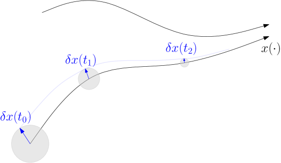
Figure 6: The convergence of infinitesimal neighboring trajectories towards each other is captured by the asymptotic stability of the linearized dynamics.

From a control-theoretic perspective, the condition (14) based on Riemannian metrics share the structure of classical Lyapunov stability with respect to quadratic Lyapunov functions. The step forward recently proposed in [24] is to view contraction analysis as a differential Lyapunov theory, allowing to consider more general (and not necessarily quadratic) Lyapunov functions in the tangent bundle.

Let $\mathcal{X}$ be the state-space of the system represented by $\dot{x}=f(x)$, and consider the prolonged system [17] represented by the pairing of the system dynamics with the linearized dynamics

$$\left\{\begin{array}[]{rcl}\dot{x}&=&f(x)\\ \dot{\delta x}&=&\partial f(x)\delta x\\ \end{array}\right.\qquad(x,\delta x)\in T\mathcal{X}\ .$$ (16)

$T\mathcal{X}$ denotes the tangent bundle of $\mathcal{X}$. In analogy with classical Lyapunov theory, a Finsler-Lyapunov function from the tangent bundle $T\mathcal{X}$ to ${\mathbb{R}}_{\geq 0}$ satisfies the bounds

$$c_{1}|\delta x|_{x}^{p}\leq V(x,\delta x)\leq c_{2}|\delta x|_{x}^{p}$$ (17)

where $c_{1},c_{2}\in{\mathbb{R}}_{>0}$, $p$ is some positive integer and $|\cdot|_{x}$ is a Finsler metric. Intuitively, $|\cdot|_{x}$ defines a Minkowski norm in each tangent space $T_{x}\mathcal{X}$, [13] From (17), a Finsler-Lyapunov function measures the length of any tangent vector $\delta x$. In other words, $V$ is a measure of the distance of $\delta x$ from $0$, providing to the linearized dynamics the equivalent of a classical Lyapunov function, typically measuring the distance of the state $x$ from the $0$ equilibrium.

The stability of the linearized dynamics along the system trajectories follows from the pointwise decay of the Finsler-Lyapunov function along the trajectories of the prolonged system. Geometrically, one has to establish

$$\dot{V}\leq-\alpha(V(x,\delta x))$$ (18)

where $\dot{V}$ reads $\partial_{x}V(x,\delta x)f(x)+\partial_{\delta x}V(x,\delta x)\partial f(x)\delta x$ and $\alpha$ is a $\mathcal{K}$ function. (17) and (18) guarantee that the nonlinear system is contractive (15) but with respect to the Finslerian distance $d$ induced by the Finsler metric $|\cdot|_{x}$, by integration, [24, Theorem 1]. A straightforward corollary is that any fixed point of the nonlinear system is necessarily unique and globally asymptotically stable.

(17) and (18) subsume many conditions for contraction available in the literature, [39, 40, 3, 1, 48, 34, 55, 59]. For a detailed comparison, please refer to [24, Section VI]. See also [2] for a discussion on the basic concepts of contraction theory.

(17) and (18) allows for the analysis of time-varying systems $\dot{x}=f(x,t)$, for which $\dot{V}$ reads $\partial_{x}V(x,\delta x)f(x,t)+\partial_{\delta x}V(x,\delta x)\partial_{x}f(x,t)\delta x$. The notion of Finsler-Lyapunov function in (17) can be further generalized to time-varying functions $V$, modifying accordingly (18). By exploiting the analogy with classical Lyapunov theory, under boundedness assumption on the trajectories of the (time-invariant) nonlinear system $\dot{x}=f(x)$, (18) can be relaxed to the LaSalle-like formulation

$$\dot{V}\leq-\alpha(x,\delta x)$$ (19)

where $\alpha:T\mathcal{X}\to{\mathbb{R}}_{\geq 0}$. Then, the contraction property (15) holds provided that the largest invariant set contained in

$$\Pi(x,\delta x):=\{(x,\delta x)\in T\mathcal{X}\,|\,\alpha(x,\delta x)=0\}$$ (20)

is given by $\mathcal{X}\times\{0\}$, [24, Theorem 2].

IV-C Differential analysis of the overdamped pendulum

The overdamped pendulum (8) is studied in [24] via differential analysis. For $u=0$, the simple choice of the Finsler-Lyapunov function $V:=\delta\vartheta^{2}$ guarantees that

$$\dot{V}=-\cos(\vartheta)\delta\vartheta^{2}<0\qquad\forall(\vartheta,\delta\vartheta)\in\left(-\frac{\pi}{2},\frac{\pi}{2}\right)\times{\mathbb{R}}.$$ (21)

The decay of the Finsler-Lyapunov function is restricted to the open lower half of the circle. Thus, the contraction (15) holds only among those trajectories of the nonlinear dynamics whose image is contained within $\left(-\frac{\pi}{2},\frac{\pi}{2}\right)$ (forward invariant region). The particular selection of a constant Finsler-Lyapunov function with respect to $\vartheta$ (in coordinates) makes the condition $\dot{V}<0$ feasible only within the region of strict monotonicity of the vector field $\dot{\vartheta}=-\sin(\vartheta)$. For instance, this is the result that one would obtain by considering the convergence to zero of the arc length $\Delta\vartheta:=\vartheta_{1}-\vartheta_{2}$, where $\vartheta_{1},\vartheta_{2}$ both satisfy the overdamped pendulum dynamics.

The Finsler-Lyapunov function $V:=\frac{\delta\vartheta^{2}}{1+\cos(\vartheta)}$ deforms the measure of the length of $\delta\vartheta$ as a function of the particular point $\vartheta$, establishing contraction beyond monotonicity of the right-hand side of overdamped pendulum equations. For this new Finsler-Lyapunov function (18) reads

$$\dot{V}=-\delta\vartheta^{2}<0\qquad\forall(\vartheta,\delta\vartheta)\in\left(-\pi,\pi\right)\times{\mathbb{R}},$$ (22)

that is, for all the points of the circle but the unstable point at $\pi$. From (15), it is clear that the exclusion of the unstable fixed point is a necessary condition to achieve the decay of the Finsler-Lyapunov function, since no trajectory converges to the steady-state trajectory $\pi$. Looking at Figure 7, the intuitive explanation for (22) is that the distance $d$ associated to the new Finsler-Lyapunov function by integration of the Finsler metric $\left(\frac{\delta x^{2}}{1+\cos(\vartheta)}\right)^{\!\frac{1}{2}}$ measures constant arc length intervals $b-a=c-b=\mathit{const}$ in a way that guarantees $d(a,b)<d(b,c)$, following a transformation similar to the one represented in Figure 7.

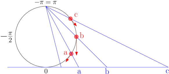
Figure 7: A representation of the geodesic distance induced by the Finsler metric $\sqrt{\frac{\delta x^{2}}{1+\cos(\vartheta)}}$ on the circle.

It is insightful to look at the overdamped pendulum under the feedforward action of the (possibly non-constant) torque $u\neq 0$, to illustrate the use of Finsler-Lyapunov functions away from the study of stability of fixed points. (2) with $\delta u=0$ characterize the linearized dynamics along any trajectory $(\vartheta(\cdot),v(\cdot))$ generated by the action of the input $u(\cdot)$. In fact, for $\delta u=0$, the linearization captures the infinitesimal mismatch between $(\vartheta(\cdot),v(\cdot))$ and any other neighboring trajectory generated by the same input $u(\cdot)$. For the pendulum, the presence of the input changes the pointwise decay (22) into

$$\dot{V}=-\delta\vartheta^{2}+w(\vartheta,\delta\vartheta,u)\qquad\forall(\vartheta,\delta\vartheta)\in\left(-\pi,\pi\right)\times{\mathbb{R}},$$ (23)

where the term $w$ is not sign definite. Indeed, not surprisingly, the trajectories along which the linearized dynamics are now modified by the action of the input $u$, and the decay of a non-constant Finsler-Lyapunov function designed by taking into account the specific nonlinearities of the system vector field is perturbed by the action of the input. To achieve the property of uniform asymptotic stability of the linearization - or uniform contraction - with respect to the input, the input action must be paired to the particular definition of the Finsler-Lyapunov function. For example, for the overdamped pendulum, taking $u=\cos(\frac{\vartheta}{2})r$ guarantees that the inequality (22) holds uniformly in $r$, that is,

$$w(\vartheta,\delta\vartheta,\cos(\vartheta/2)r)=0$$ (24)

for all $(\vartheta,\delta\vartheta)\in\left(-\pi,\pi\right)\times{\mathbb{R}}$ and all $r\in{\mathbb{R}}$, as detailed in [26, Example 1].

The uniform contraction of the overdamped pendulum is illustrated by the simulations in Figure 8, for small and large sinusoidal signals $r$. Uniform contraction with respect to the input is a powerful property, at the core of many results in contraction-based design [40, 49, 50, 47, 55, 63, 26]. A uniform contracting system behaves like a filter: it forgets the initial conditions and its trajectories asymptotically converge to the unique, globally attractive steady state compatible with the input signal, for any given input signal injected into the system.

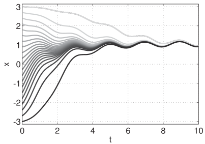
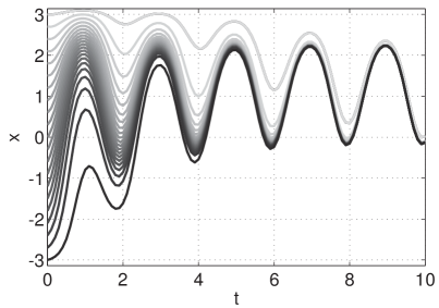
Figure 8: Entrainment of the overdamped pendulum for $u=\cos(\frac{\vartheta}{2})r$ and oscillating exogenous signal $r=1+\gamma\sin(\pi t)$, for constant gain $\gamma$ small (left) and large (right).

Uniform contraction is also at the root of several contributions on the interconnection of contractive nonlinear systems. As in classical control, the system arising from the interconnection of contractive systems is not necessarily contractive. The results available in the literature extend to the differential framework classical cascade and small gain approaches [63, 56, 59] and dissipativity theory [66, 23, 26]. For example, without entering into the details of the analysis (the reader is referred to [26, Example 1]), the overdamped pendulum with $u=\cos(\frac{\vartheta}{2})r$ is differentially passive from $r$ to the (differentially) passivating output $y:=\int_{0}^{\vartheta}\sec(\frac{s}{2})ds$, that is,

$$\dot{V}\leq\delta r\delta y\ .$$ (25)

In analogy with classical passivity in Section II-B, $V$ has the role here of differential storage whose variation is bounded by the differential supply $\delta r\delta y$.

The analogy with classical passivity goes beyond basic definitions: the negative feedback interconnection of differentially passive systems is differentially passive. Thus, for example, the closed loop of the overdamped pendulum with any strictly increasing static nonlinearity $r=-h(y)$, that is, $\delta r=\partial h(y)\delta y$ with $\partial h(y)>0$, leads to a contractive dynamics. Figure 9 illustrates the behavior of the contractive system arising from the interconnection of two overdamped pendulums.

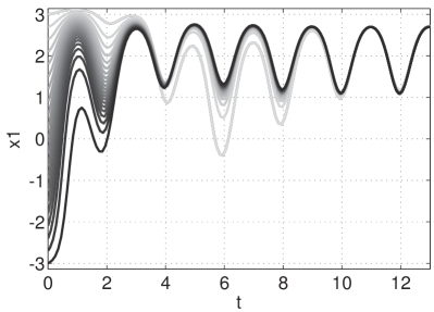
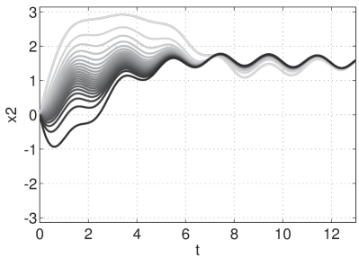
Figure 9: Feedback interconnection $r_{1}=-y_{2}+q_{1}$, $r_{2}=y_{1}+q_{2}$ of two differentially passive overdamped pendulums, where the indices $1$ and $2$ on the variables indicates respectively the variables of the first (left) and second (right) pendulum. The simulations illustrate the behavior of the interconnected dynamics for a sinusoidal exogenous signal $q_{1}=1+\gamma\sin(\pi t)$ and for a constant signal $q_{2}=0$, for different initial conditions of the first pendulum (left).

IV-D Horizontal contraction

Contraction theory shows how a differential analysis can infer global properties of the incremental dynamics from the linearized system. It opens a number of possibilities to study the incremental stability properties required by questions including nonlinear regulation, tracking, observer design, and synchronization.

It is however well recognized that the contraction property is the exception rather than the rule in most applications because a number of system properties preclude contraction along some directions of the tangent space. A system with conserved quantities or symmetries cannot be a contraction because no contraction is allowed along the symmetry directions. A system with a limit cycle cannot be a contraction because no contraction is allowed along the closed orbit of an autonomous system. Horizontal contraction generalizes the differential analysis to such situations by decomposing each tangent space into a vertical component where contraction is not required and a horizontal space where contraction is required. The recent paper [24] explores particular situations where this local decomposition can lead to a global analysis of the behavior.

Within the differential Lyapunov theory, weak forms of contraction can be easily introduced by weakening (17) to the inequalities

$$c_{1}|\pi(x)\delta x|_{x}^{p}\leq V(x,\delta x)\leq c_{2}|\pi(x)\delta x|_{x}^{p}$$ (26)

where, for every $x\in\mathcal{X}$, $\pi(x)$ is a linear projection that maps the tangent vectors of $T_{x}\mathcal{X}$ into the horizontal subspace $\mathcal{H}_{x}\subset T_{x}\mathcal{X}$. In local coordinates $\pi(x)$ is a matrix whose elements are smooth functions of $x$. Its columns provide a horizontal distribution spanning $\mathcal{H}_{x}$. The vertical space $\mathcal{V}_{x}$ is thus defined by the vectors $\delta x\in T_{x}\mathcal{X}$ such that $\pi(x)\delta x=0$.

The combination of (26) and (18) establishes a contraction property confined to the directions spanned by the horizontal distribution. It opens the way to the use of the differential Lyapunov theory in the presence of symmetry directions along which no contraction is expected, [24, Section VII]. Figure 10 provides an illustration of the approach. The transversality of the horizontal space (in blue) with respect to the motion along the limit cycle $\Omega$ (in black) allows to disregard the lack of contraction in the direction of the vector field of the system (in red). Indeed, in a small neighborhood of the limit cycle, the integral manifold of the horizontal distribution at $x\in\Omega$ is a Poincaré section (see Figure 5).

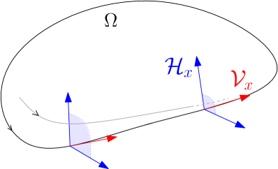
Figure 10: Horizontal contraction decomposes the tangent space into a horizontal space (blue) and a vertical space (red). Contraction is established along the horizontal directions only.

Several examples of weak contraction for limit cycle analysis and synchronization can be found in [51, 57, 56, 24, 41]. The property introduced in the next section is also a form of horizontal contraction that is relevant for the pendulum analysis.

V Differential positivity: local order and simple attractors

V-A A differential view on monotone systems

Monotone dynamical systems [61, 31] are dynamical systems whose trajectories preserve some partial order relation $\preceq_{\mathcal{K}}$ on the state space. Partial orders are usually defined from cones. Let $\mathcal{V}$ be the vector state-space of the system and consider a (pointed convex solid) cone $\mathcal{K}\subseteq\mathcal{V}$. For any given $x_{1},x_{2}\in\mathcal{V}$, the partial order $\preceq_{\mathcal{K}}\subseteq\mathcal{V}\times\mathcal{V}$ satisfies

$$x_{1}\preceq_{\mathcal{K}}x_{2}\quad\mbox{iff}\quad x_{2}-x_{1}\in\mathcal{K}\ .$$ (27)

From (27), monotonicity reads as follow. For any initial time $t_{0}$, any pair of trajectories $x_{1}(\cdot),x_{2}(\cdot)$ of a monotone system satisfies

$$x_{1}(t_{0})\preceq x_{2}(t_{0})\ \Rightarrow\ x_{1}(t)\preceq x_{2}(t)\quad\forall t\geq t_{0}$$ (28)

Through the introduction of a partial order relation on the input space, the notion of monotonicity easily extends to open systems, as illustrated in [5].

Monotone systems include the class of cooperative and competitive systems [32, 52] and play a fundamental role in chemical and biological applications [4, 19, 20, 62, 9, 10]. They enjoy important convergence properties [61, 30, 43, 7, 8, 12] and interesting interconnections properties [5, 6, 21].

A crucial observation is that monotonicity of a system $\dot{x}=f(x)$ is equivalent to the positivity of the linearized dynamics $\dot{\delta x}=\partial f(x)\delta x$. Positivity is intended here in the sense of cone invariance [15]: for any initial time $t_{0}$ the trajectories $\delta x(\cdot)$ of the linearized positive dynamics satisfy the implication

$$\delta x(t_{0})\in\mathcal{K}\ \Rightarrow\ \delta x(t)\in\mathcal{K}\quad\forall t\geq t_{0}\ .$$ (29)

An intuitive explanation of the connection between positivity and monotonicity follows from the analysis of the mismatch between infinitesimally neighboring solutions $x_{2}(\cdot):=x_{1}(\cdot)+\delta x(\cdot)$ of the nonlinear dynamics $\dot{x}=f(x)$, where $\delta x(\cdot)$ is driven by the linearized dynamics $\dot{\delta x}(t)=\partial_{x}f(x_{1}(t))\delta x(t)$. The combination of (27) and (28) gives

$$x_{2}(t_{0})-x_{1}(t_{0})\in\mathcal{K}\ \Rightarrow\ x_{2}(t)-x_{1}(t)\in\mathcal{K}\quad\forall t\geq t_{0}\$$ (30)

which leads to (29) because of the identity $\delta x(\cdot)=x_{2}(\cdot)-x_{1}(\cdot)$. The route from (28) to (29) is at the core of the equivalence between closed cooperative systems and the Kamke condition [61, Chapter 3], and of the equivalence between open cooperative systems and the notion of incrementally positive systems introduced in [5, Section VIII].

We anticipate that a suitably extended notion of positivity, detailed in the next section, is the source of several convergence properties of monotone systems. Again, a property of the linearization (positivity) underlies a property of the nonlinear system (monotonicity)

V-B Positive linearizations

Positive systems are linear behaviors that leave a cone invariant [15]. Rephrasing (29), the linear system $\dot{x}=Ax$ is positive with respect to a cone $\mathcal{K}$ if

$$e^{At}\mathcal{K}\subseteq\mathcal{K}\qquad\forall t>0\ ,$$ (31)

where $e^{At}\mathcal{K}:=\{e^{At}x\,|\,x\in\mathcal{K}\}$. Positive systems have a rich history because positivity strongly restricts the behavior of the system, as established by the Perron-Frobenius theory: under mild extra assumptions ensuring that the the transition matrix $e^{At}$ maps the boundary of the cone into the interior, any trajectory $e^{At}x$, $x\in\mathcal{K}$, converges asymptotically to a one dimensional subspace spanned by the eigenvector associated to the (real) eigenvalue of largest real part of the state matrix $A$, [15]. This convergence follows from the fact that positive systems enjoy a projective contraction property which has been exploited in a number of applications, ranging from stabilization [70, 45, 22, 18, 36, 54] to observer design [29, 14], and to distributed control [44, 53, 58].

For nonlinear dynamics, the crucial observation is that positivity of the linearization strongly restricts also the nonlinear behaviors. For dynamics on manifolds $\mathcal{X}$, positivity must be intended in a generalized sense, compatible with the fact that the prolonged system $\dot{x}=f(x)$, $\dot{\delta x}=\partial f(x)\delta x$ lives in the tangent bundle $T\mathcal{X}$. The cone of linear positivity becomes a (smooth) cone field given by a (pointed convex solid) cone $\mathcal{K}(x)\subseteq T_{x}\mathcal{X}$ attached to each $x$. The nonlinear dynamics is differentially positive if the cone field is invariant along the trajectories of the (prolonged) system, that is,

$$\partial\psi_{t}(x)\mathcal{K}(x)\subseteq\mathcal{K}(\psi_{t}(x))\qquad\forall x\in\mathcal{X},\forall t\geq 0$$ (32)

where $\psi_{t}(x)$ denotes the flow of $\dot{x}=f(x)$ at time $t$ from the initial condition $x$, and $\partial\psi_{t}(x)$ denotes the differential $\partial_{x}\psi_{t}(x)$ computed at $x$, [25, Section 5]. Note that for any initial condition $(x,\delta x)\in T\mathcal{X}$ the pair $(\psi_{t}(x),\partial\psi_{t}(x)\delta x)$ is a trajectory of the prolonged system. Differential positivity (32) reduces to positivity (31) on linear dynamics and constant cone fields.

Figure 11 illustrates three different phase portraits of differentially positive systems. One of the phase portraits is represented in two different set of coordinates. The systems in Figure 11.I and Figure 11.II are differentially positive with respect to a constant cone field on a vector space. The system on the left is a linear positive system. The one on the right is a monotone system whose partial order relation $\preceq$ is the usual element-wise order. Indeed, every differentially positive system with respect to a constant cone field on a vector space is a monotone system with respect to the order $x\preceq_{\mathcal{K}}y\mbox{ iff }y-x\in\mathcal{K}$. The harmonic oscillator in Figure 11.III is neither a positive system, nor a monotone system, but it is a differentially positive system with respect to a non constant cone field rotating with the flow. In polar coordinates, that is, on the nonlinear space ${\mathbb{R}}_{+}\times\mathbb{S}$, the coordinate representation of the cone field in each tangent space is constant.

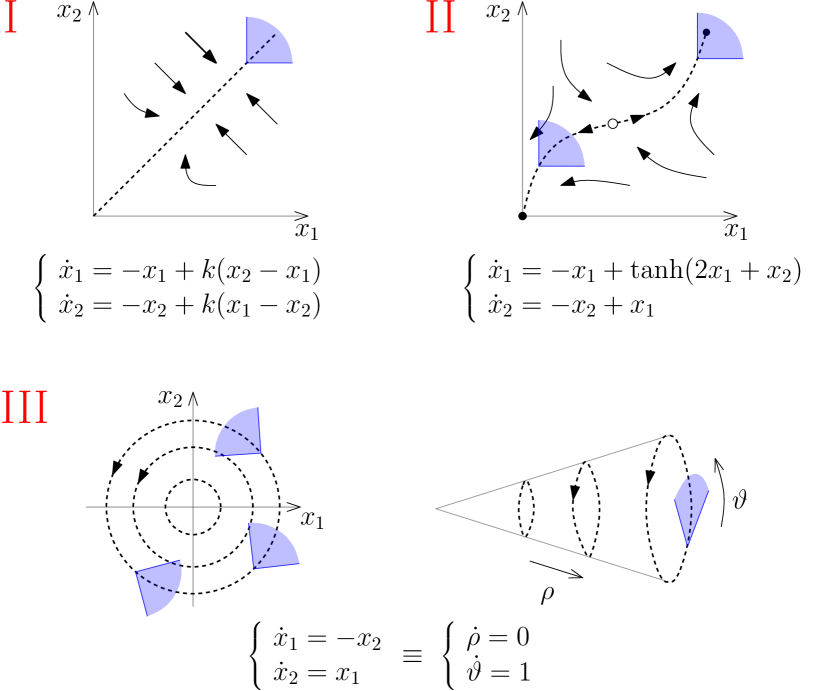
Figure 11: The phase portraits of three different planar differentially positive systems. (I) a linear consensus model. (II) a monotone bistable model. (III) the harmonic oscillator.

Differentially positive systems inherit many properties of positivity, under some mild extra conditions ensuring that the the differential $\partial\psi_{T}(x)$ maps uniformly the boundary of the cone at $x$ into the interior of the cone $\mathcal{K}(\psi_{T}(x))$ for some $T>0$ (see the notion of uniform strict differential positivity in [25]). In particular, the projective contraction of positive systems extends to differentially positive systems, leading to the definition of the so called Perron-Frobenius vector field $w(x)$ [25, Theorem 2], a continuous vector field direct generalization of the Perron-Frobenius dominant eigenvector of linear positivity. Indeed, consider the distribution $\mathcal{W}(x):=\{\lambda w(x)\,|\,\lambda\in{\mathbb{R}}\}\subset T_{x}\mathcal{X}$ spanned by the Perron-Frobenius vector field $w(x)$. For any trajectory $\psi_{t}(x)$, the distribution spanned by $\mathcal{W}(\psi_{t}(x))$ is an attractor for the linearized dynamics along the trajectory [25, Theorem 1], that is, for any $\delta x\in\mathcal{K}(x)$,

$$\partial\psi_{t}(x)\delta x\to\mathcal{W}(\psi_{t}(x))\mbox{ as }t\to\infty\ .$$ (33)

The identity $f(\psi_{t}(x))=\partial\psi_{t}(x)f(x)$, (33) guarantees that if $f(x)\in\mathcal{K}(x)$ then the system vector field along $\psi_{t}(x)$, satisfies

$$f(\psi_{t}(x))\to\mathcal{W}(\psi_{t}(x))\mbox{ as }t\to\infty\ .$$ (34)

The reader will immediately recognize that the asymptotic alignment of the vector field to the Perron-Frobenius vector field must constrain the steady-state behavior of differentially positive systems. In fact, exploiting (33) and (34) [25, Theorem 3] establishes that the limit behavior of a differentially positive system is either described by integral curves of the Perron-Frobenius vector field, or it is a pathological behavior, where the motion is transversal to the Perron-Frobenius vector field, leading possibly to chaotic attractors. Precisely, for every $x\in\mathcal{X}$, the $\omega$-limit set $\omega(x)$ satisfies one of the following two properties:

• The vector field $f(z)$ is aligned with the Perron-Frobenius vector field $w(z)$ for each $z\in\omega(x)$, and $\omega(x)$ is either a fixed point or a limit cycle or a set of fixed points and connecting arcs;

• The vector field $f(z)$ is nowhere aligned with the Perron-Frobenius vector field $w(z)$ for each $z\in\omega(x)$, and either $\liminf\nolimits\limits_{t\to\infty}|\partial\psi_{t}(z)w(z)|_{\psi_{t}(z)}=\infty$ or $\lim\nolimits\limits_{t\to\infty}f(\psi_{t}(z))=0$.

The dichotomy of the limit behaviors has interesting implications (see [25, Section VII]). For example, the characterization above allows to show that the trajectories of a differentially positive system with constant cone field on a vector space converge from almost every initial condition to a fixed point, indeed recovering the well-known property of almost global convergence of (strict) monotone dynamics, [30, 61]. Another interesting implication concerns limit cycles analysis. Any compact forward invariant region $\mathcal{C}\subseteq\mathcal{X}$ that does not contain fixed points, and such that $f(x)$ belongs to the interior of $\mathcal{K}_{\mathcal{X}}(x)$ for any $x\in\mathcal{C}$, necessarily contains a unique attractive periodic orbit, [25, Corollary 2]. See Figure 12 for an illustration. The result shows the potential of differential positivity for the analysis of limit cycles in possibly high dimensional spaces.

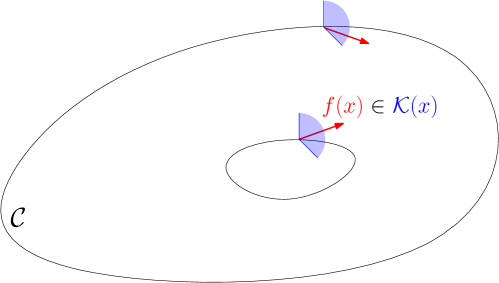
Figure 12: (Strict) Differential positivity guarantees the existence of an isolated and attractive limit cycle in every compact forward invariant region $\mathcal{C}$ that does not contain any fixed point and satisfies the condition that $f(x)$ belongs to the interior of $\mathcal{K}_{\mathcal{X}}(x)$ for any $x\in\mathcal{C}$.

V-C Differential positivity of the nonlinear pendulum

For values of the damping $k$ greater than $2$, the (strict) differential positivity of the pendulum can be established by looking at the state matrix $A(\vartheta,k)$ in (2). The invariant cone field reads

$$\mathcal{K}(\vartheta,v):=\{(\delta\vartheta,\delta v)\in T_{(\vartheta,v)}\mathcal{X}\,|\,\delta\vartheta\geq 0,\delta\vartheta+\delta v\geq 0\}\ ,$$ (35)

represented by the shaded region in Figure 13. The invariance follows from the observation that for any $\delta x=[\ \delta\vartheta\ \ \delta v\ ]^{T}$ on the boundary of the cone, the vector field of the linearized dynamics $A(\vartheta,k)\delta x$ is oriented towards the interior of the cone for any value of $\vartheta$, as represented by the black arrows attached to the boundary of the cone in Figure 13. The blue and the red lines in Figure 13 show the direction of the eigenvectors of $A(\vartheta,4)$ (left) - $A(\vartheta,3)$ (center) - $A(\vartheta,2)$ (right), for sampled values of $\vartheta\in\mathbb{S}$. The red eigenvectors are related to the largest eigenvalues and play the role of attractors for the linearized dynamics. The projective contraction holds for $k>2$ and it is lost at $k=2$, for which the state matrix $A(0,2)$ has two eigenvalues in $-1$ that makes the positivity of the linearized system on the equilibrium at $0$ (for $u=0$) non strict.

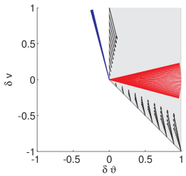
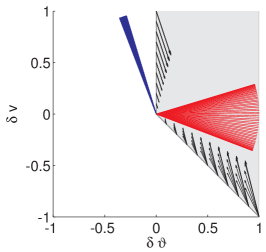
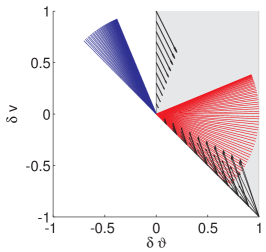
Figure 13: $\mathcal{K}(\vartheta,v)$ is shaded in gray. The two eigenvector of $A(\vartheta,k)$ for a selection $\vartheta\in\mathbb{S}$ are represented in red and blue. Red eigenvectors - largest eigenvalues. Blue eigenvectors - smallest eigenvalues. Left figure: $k=4$. Center figure: $k=3$. Right figure: $k=2$.

For $k>2$ the trajectories of the pendulum are bounded. In particular, the kinetic energy $E:=\frac{v^{2}}{2}$ satisfies $\dot{E}=-kv^{2}+v(u-\sin(\vartheta))\leq(|u|+1-k|v|)|v|<0$, which guarantees finite time convergence of the velocity component towards the set $\mathcal{V}:=\{v\in{\mathbb{R}}\,|\,-\rho\frac{|u|+1}{k}\leq v\leq\rho\frac{|u|+1}{k}\}$ for any given $\rho>1$.

The compactness of the set $\mathbb{S}\times\mathcal{V}$ opens the way to the use of the results of the previous section. For $u=1+\varepsilon$, $\varepsilon>0$, we have that $\dot{v}\geq\varepsilon-kv$ which, after a transient, guarantees that $\dot{v}>0$, thus eventually $\dot{\vartheta}>0$. Denoting by $f(\vartheta,v)$ the right-hand side in (1), it follows that, after a finite amount of time, every trajectory belongs to a forward invariant set $\mathcal{C}\subseteq\mathbb{S}\times\mathcal{V}$ such that $f(\vartheta,v)$ belongs to the interior of $\mathcal{K}(\vartheta,v)$. Thus, the region $\mathcal{C}$ contains an isolated and attractive limit cycle.

V-D Differential positivity and homoclinic orbits

Besides projective contraction, differential positivity introduces a local order on the system dynamics that is not compatible with specific behaviors, like the existence of classes of homoclinic orbits. In particular, it rules out the existence of homoclinic orbits like the one illustrated in Figure 4. In view of the discussion of Section III.C, this means that differential positivity rules out a main route to complex attractors by imposing locally a partial order on solutions. The intuitive explanation is based on the fact that the linearization along a specific trajectory is an approximation of the mismatch between the specific trajectory and the neighboring ones. Within this interpretation, the invariance property of the cone field enforces on the system state space a local order relation that must be preserved among neighboring trajectories. For instance, on vector spaces for simplicity, consider an homoclinic orbit like the one described by the dashed line in Figure 14. The red arrows represent the direction of the Perron-Frobenius vector field. We show that such a homoclinic orbit is not compatible with differential positivity. Take two initial conditions $x$ and $x+\varepsilon\delta x$, $\varepsilon>0$ small, such that $x$ and $x+\varepsilon\delta x$ belong to the unstable manifold of the saddle point, in an infinitesimal neighborhood $\mathcal{U}$ of the saddle point. For $\mathcal{U}$ sufficiently small, by continuity, $\delta x\in\mathcal{K}(x)$ since the Perron-Frobenius vector field at the saddle point is tangent to the unstable manifold of the saddle. For $\varepsilon$ sufficiently small, the trajectories $\psi_{t}(x)$ and $\psi_{t}(x+\varepsilon\delta x)$ satisfy $\psi_{t}(x+\varepsilon\delta x)-\psi_{t}(x)\simeq\varepsilon\partial\psi_{t}(x)\delta x\in\mathcal{K}(\psi_{t}(x))$ for $t\geq 0$. Moreover, because of the homoclinic orbit, for some $t>0$, $\psi_{t}(x)$ and $\psi_{t}(x+\varepsilon\delta x)$ return to the saddle point along the stable manifold, thus necessarily breaking the relation $\psi_{t}(x+\varepsilon\delta x)-\psi_{t}(x)\in\mathcal{K}(\psi_{t}(x))$. The invariance property on the cone field necessarily fails.

[25, Corollary 3] claims that under (strict) differential positivity, any homoclinic orbit of a hyperbolic fixed point cannot be tangent to the Perron-Frobenius vector field $w(x)$ for any $x$ on the orbit. The claim is well illustrated in Figure 14. The stable and unstable manifolds of the saddle have dimension 1 and 2, respectively. The homoclinic orbit on the right part of the figure (dashed line) is ruled out by the local order at the saddle point. Rephrasing the argument above, along the whole dashed orbit the vector field $f(x)$ must be parallel along the whole Perron-Frobenius vector field $w(x)$, which violates continuity of the Perron-Frobenius vector field at the saddle point. The limit set given by the homoclinic orbit on the left part of the figure (solid line) is instead compatible with differential positivity, but the Perron-Frobenius vector field is necessarily nowhere tangent to the curve.

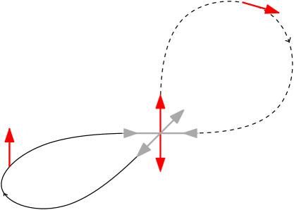
Figure 14: Two examples of homoclinic orbits. The dashed one is ruled out by (strict) differential positivity. The left one is compatible with differential positivity. The red vectors represent the direction of the Perron-Frobenius vector field.

This analysis has a direct consequence on the pendulum example. Looking at Figure 3, the differential positivity of the pendulum for $k\geq 2$ cannot be extended to values of the damping $k<k_{c}$ because of the presence of a homoclinic bifurcation for suitably selected values of the torque. Still, differential positivity might hold within the invariant subregions of the system state space separated by the homoclinic orbit.

VI Conclusion

Differential analysis aims at exploiting the (local) properties of linearized dynamics to infer (global) properties of nonlinear behaviors. It is especially relevant for the analysis of nonlinear models defined by nonlinear vector fields on nonlinear spaces. The tutorial paper has illustrated on the nonlinear pendulum example reasons why several nonlinear control problems require an analysis of the incremental dynamics and the potential of differential analysis to address such questions. Emphasis was put on recent developments by the authors in differential analysis [24, 25]. Horizontal contraction and differential positivity illustrate the potential of a differential analysis beyond the global analysis of an equilibrium solution. It is hoped that the insight provided by a differential analysis in an archetype model such as the nonlinear pendulum will stimulate the potential relevance of this approach in more challenging control applications.

References

- [1] N. Aghannan and P. Rouchon. An intrinsic observer for a class of lagrangian systems. IEEE Transactions on Automatic Control, 48(6):936 – 945, 2003.
- [2] Z. Aminzare and E.D. Sontag. Contraction methods for nonlinear systems: A brief introduction and some open problems. In 53rd IEEE Conference of Decision and Control, Los Angeles, 2014. To appear.
- [3] D. Angeli. A Lyapunov approach to incremental stability properties. IEEE Transactions on Automatic Control, 47:410–421, 2000.
- [4] D. Angeli, J.E. Ferrell, and E.D. Sontag. Detection of multistability, bifurcations, and hysteresis in a large class of biological positive-feedback systems. Proceedings of the National Academy of Sciences of the United States of America, 101(7):1822–1827, 2004.
- [5] D. Angeli and E.D. Sontag. Monotone control systems. IEEE Transactions on Automatic Control, 48(10):1684 – 1698, 2003.
- [6] D. Angeli and E.D. Sontag. Interconnections of monotone systems with steady-state characteristics. In MarcioS. Queiroz, Michael Malisoff, and Peter Wolenski, editors, Optimal Control, Stabilization and Nonsmooth Analysis, volume 301 of Lecture Notes in Control and Information Science, pages 135–154. Springer Berlin Heidelberg, 2004.
- [7] D. Angeli and E.D. Sontag. Multi-stability in monotone input/output systems. Systems & Control Letters, 51(3–4):185 – 202, 2004.
- [8] D. Angeli and E.D. Sontag. A note on monotone systems with positive translation invariance. In 14th Mediterranean Conference on Control and Automation, 2006. MED ’06., pages 1–6, 2006.
- [9] D. Angeli and E.D. Sontag. Translation-invariant monotone systems, and a global convergence result for enzymatic futile cycles. Nonlinear Analysis: Real World Applications, 9(1):128 – 140, 2008.
- [10] D. Angeli and E.D. Sontag. Remarks on the invalidation of biological models using monotone systems theory. In Proceedings of the 51st IEEE Conference on Decision and Control (CDC), pages 2989–2994, 2012.
- [11] L. Arnold and V. Wihstutz. Lyapunov Exponents. Lecture Notes in Mathematics. Springer, 1 edition, 1986.
- [12] M. Banaji and D. Angeli. Convergence in strongly monotone systems with an increasing first integral. SIAM Journal on Mathematical Analysis, 42(1):334–353, 2010.
- [13] D. Bao, S.S. Chern, and Z. Shen. An Introduction to Riemann-Finsler Geometry. Springer-Verlag New York, Inc. (2000), 2000.
- [14] S. Bonnabel, A. Astolfi, and R. Sepulchre. Contraction and observer design on cones. In Proceedings of 50th IEEE Conference on Decision and Control and European Control Conference, pages 7147–7151, 2011.
- [15] P.J. Bushell. Hilbert’s metric and positive contraction mappings in a Banach space. Archive for Rational Mechanics and Analysis, 52(4):330–338, 1973.
- [16] M. Chamberland. Global asymptotic stability, additive neural networks, and the Jacobian conjecture. Canadian applied Mathematics Quarterly, 5(4):331–339, 1997.
- [17] P.E. Crouch and A.J. van der Schaft. Variational and Hamiltonian control systems. Lecture notes in control and information sciences. Springer, 1987.
- [18] P. De Leenheer and D. Aeyels. Stabilization of positive linear systems. Systems & Control Letters, 44(4):259 – 271, 2001.
- [19] P. De Leenheer, D. Angeli, and E.D. Sontag. A tutorial on monotone systems - with an application to chemical reaction networks. In Proceedigns f the 16th International Symposium Mathematical Theory of Networks and Systems, 2004.
- [20] P. De Leenheer, D. Angeli, and E.D. Sontag. Monotone chemical reaction networks. Journal of Mathematical Chemistry, 41(3):295–314, 2007.
- [21] G. Enciso and E.D. Sontag. Monotone systems under positive feedback: multistability and a reduction theorem. Systems & Control Letters, 54(2):159 – 168, 2005.
- [22] L. Farina and S. Rinaldi. Positive linear systems: theory and applications. Pure and applied mathematics (John Wiley & Sons). Wiley, 2000.
- [23] F. Forni and R. Sepulchre. On differentially dissipative dynamical systems. In 9th IFAC Symposium on Nonlinear Control Systems, 2013.
- [24] F. Forni and R. Sepulchre. A differential Lyapunov framework for contraction analysis. IEEE Transactions on Automatic Control, 59(3):614–628, 2014.
- [25] F. Forni and R. Sepulchre. Differentially positive systems. Submitted to IEEE Transactions on Automatic Control (Available at http://arxiv.org/abs/1405.6298v1), 2014.
- [26] F. Forni, R. Sepulchre, and A.J. van der Schaft. On differential passivity of physical systems. In 52nd IEEE Conference on Decision and Control, 2013.
- [27] Leonov. G.A., N.V. Kuznetsov, and V.O. Bragin. On problems of aizerman and kalman. Vestnik St. Petersburg University: Mathematics, 43, 2010.
- [28] J. Guckenheimer and P. Holmes. Nonlinear Oscillation, Dynamical Systems and Bifurcations of Vector Fields. Applied Mathematical Sciences. Springer, second, rev, corr edition, 1983.
- [29] H.M. Hardin and J.H. van Schuppen. Observers for linear positive systems. Linear Algebra and its Applications, 425(2–3):571 – 607, 2007.
- [30] M.W. Hirsch. Stability and convergence in strongly monotone dynamical systems. Journal für die reine und angewandte Mathematik, 383:1–53, 1988.
- [31] M.W. Hirsch. Fixed points of monotone maps. Journal of Differential Equations, 123(1):171 – 179, 1995.
- [32] M.W. Hirsch and H.L. Smith. Competitive and cooperative systems: A mini-review. In L. Benvenuti, A. Santis, and L. Farina, editors, Positive Systems, volume 294 of Lecture Notes in Control and Information Science, pages 183–190. Springer Berlin Heidelberg, 2003.
- [33] A. Isidori. Nonlinear Control Systems. Number v. 1 in Communications and Control Engineering. Springer, 1995.
- [34] J. Jouffroy. Some ancestors of contraction analysis. In 44th IEEE Conference on Decision and Control, 2005 and 2005 European Control Conference. CDC-ECC ’05., pages 5450 – 5455, dec. 2005.
- [35] R.E. Kalman. Physical and mathematical mechanisms of instability in nonlinear automatic control systems. Transactions of ASME, 79(3):553–566, 1957.
- [36] F. Knorn, O. Mason, and R Shorten. On linear co-positive Lyapunov functions for sets of linear positive systems. Automatica, 45(8):1943 – 1947, 2009.
- [37] G. A. Leonov, G.A. and N.V. Kuznetsov. Time-varying linearization and the Perron effects. International Journal of Bifurcation and Chaos, 17(04):1079–1107, 2007.
- [38] G.A. Leonov. Strange attractors and classical stability theory. Nonlinear dynamics and systems theory, 8(1):49–96, 2008.
- [39] D.C. Lewis. Metric properties of differential equations. American Journal of Mathematics, 71(2):294–312, April 1949.
- [40] W. Lohmiller and J.E. Slotine. On contraction analysis for non-linear systems. Automatica, 34(6):683–696, June 1998.
- [41] I.R. Manchester and J.J. Slotine. Transverse contraction criteria for existence, stability, and robustness of a limit cycle. Systems & Control Letters, 63(0):32 – 38, 2014.
- [42] L. Markus and H. Yamabe. Global stability criteria for differential systems. Osaka Math., 21:305–317, 1960.
- [43] J. Mierczyński. Cooperative irreducibile systems of ordinary differential equations with first integral. In Proceedings of the Second Marrakesh Conference on Differential Equations, 1995.
- [44] L. Moreau. Stability of continuous-time distributed consensus algorithms. In 43rd IEEE Conference on Decision and Control, volume 4, pages 3998 – 4003, 2004.
- [45] S. Muratori and S. Rinaldi. Excitability, stability, and sign of equilibria in positive linear systems. Systems & Control Letters, 16(1):59 – 63, 1991.
- [46] R. Ortega, A.J. Van Der Schaft, I. Mareels, and B. Maschke. Putting energy back in control. Control Systems, IEEE, 21(2):18 –33, apr 2001.
- [47] A. Pavlov and L. Marconi. Incremental passivity and output regulation. Systems and Control Letters, 57(5):400 – 409, 2008.
- [48] A. Pavlov, A. Pogromsky, N. van de Wouw, and H. Nijmeijer. Convergent dynamics, a tribute to Boris Pavlovich Demidovich. Systems & Control Letters, 52(3-4):257 – 261, 2004.
- [49] A. Pavlov, N. van de van de Wouw, and H. Nijmeijer. Uniform output regulation of nonlinear systems: A convergent dynamics approach, 2005.
- [50] A. Pavlov, N. Van de Wouw, and H. Nijmeijer. Frequency response functions for nonlinear convergent systems. IEEE Transactions on Automatic Control, 52(6):1159–1165, 2007.
- [51] Q.C. Pham and J.E. Slotine. Stable concurrent synchronization in dynamic system networks. Neural Networks, 20(1):62 – 77, 2007.
- [52] C. Piccardi and S. Rinaldi. Remarks on excitability, stability and sign of equilibria in cooperative systems. Systems & Control Letters, 46(3):153 – 163, 2002.
- [53] A. Rantzer. Distributed control of positive systems. ArXiv e-prints, 2012.
- [54] B. Roszak and E.J. Davison. Necessary and sufficient conditions for stabilizability of positive LTI systems. Systems & Control Letters, 58(7):474 – 481, 2009.
- [55] G. Russo, M. Di Bernardo, and E.D. Sontag. Global entrainment of transcriptional systems to periodic inputs. PLoS Computational Biology, 6(4):e1000739, 04 2010.
- [56] G. Russo, M. di Bernardo, and E.D. Sontag. A contraction approach to the hierarchical analysis and design of networked systems. IEEE Transactions on Automatic Control, PP(99):1–1, 2013.
- [57] G. Russo and J.J. Slotine. Symmetries, stability, and control in nonlinear systems and networks. Phys. Rev. E, 84:041929, Oct 2011.
- [58] R. Sepulchre, A. Sarlette, and P. Rouchon. Consensus in non-commutative spaces. In Proceedings of the 49th IEEE Conference on Decision and Control, CDC 2010, pages 6596–6601. IEEE, 2010.
- [59] J.W. Simpson-Porco and F. Bullo. Contraction theory on Riemannian manifolds. Systems & Control Letters, 65(0):74 – 80, 2014.
- [60] S. Smale, F. Cucker, and R. Wong. The Collected Papers of Stephen Smale: Volume 2, volume 2. World Scientific, 2000.
- [61] H.L. Smith. Monotone Dynamical Systems: An Introduction to the Theory of Competitive and Cooperative Systems, volume 41 of Mathematical Surveys and Monographs. American Mathematical Society, 1995.
- [62] E.D. Sontag. Monotone and near-monotone biochemical networks. Systems and Synthetic Biology, 1(2):59–87, 2007.
- [63] E.D. Sontag. Contractive Systems with Inputs, pages 217–228. Perspectives in Mathematical System Theory, Control, and Signal Processing. Springer-verlag, 2010.
- [64] S.H. Strogatz. Nonlinear Dynamics And Chaos. Westview Press, 1994.
- [65] A.J. van der Schaft. Port-hamiltonian systems: an introductory survey. In M. Sanz-Sole, J. Soria, J.L. Varona, and J. Verdera, editors, Proceedings of the International Congress of Mathematicians Vol. III: Invited Lectures, pages 1339–1365, Madrid, Spain, 2006. European Mathematical Society Publishing House (EMS Ph).
- [66] A.J. van der Schaft. On differential passivity. In 9th IFAC Symposium on Nonlinear Control Systems, 2013.
- [67] E.W. Weisstein. Lyapunov characteristic exponent. http://mathworld.wolfram.com/LyapunovCharacteristicExponent.html, 2014.
- [68] J.C. Willems. Dissipative dynamical systems part I: General theory. Archive for Rational Mechanics and Analysis, 45:321–351, 1972.
- [69] J.C. Willems. Dissipative dynamical systems part II: Linear systems with quadratic supply rates. Archive for Rational Mechanics and Analysis, 45:352–393, 1972.
- [70] J.C. Willems. Lyapunov functions for diagonally dominant systems. Automatica, 12(5):519–523, 1976.