Nonlinear dynamics of atoms in a crossed optical dipole trap

Abstract

We explore the classical dynamics of atoms in an optical dipole trap formed by two identical Gaussian beams propagating in perpendicular directions. The phase space is a mixture of regular and chaotic orbits, the later becoming dominant as the energy of the atoms increases. The trapping capabilities of these perpendicular Gaussian beams are investigated by considering an atomic ensemble in free motion. After a sudden turn on of the dipole trap, a certain fraction of atoms in the ensemble remains trapped. The majority of these trapped atoms has energies larger than the escape channels, which can be explained by the existence of regular and chaotic orbits with very long escape times.

I Introduction

Since the seventies, it is well known that the interaction between the induced atomic dipole moment and the intensity gradient of a non-resonant light enables the optical confinement of neutral atoms ashkin ; varios ; cable ; grimm ; MetcalfStraten . Nowadays, these optical dipole traps are routinely used to confine neutral atoms in the cold and ultracold regime where quantum-engineering is required. These confined atomic ensembles allow for a wide range of applications such as single atom manipulation PhysRevA.67.033403 , Bose-Einstein condensation bec , optical atomic clocks clocks or the observation of classical and quantum chaos PhysRevLett.86.1514 ; PhysRevLett.86.1518 .

The simplest optical trap providing confinement of neutral atoms consists of a single strongly focused Gaussian laser beam ashkin ; cable . In this case, the confinement is one-dimensional and perpendicular to the propagation of the beam axis. For a tight confinement in the three spatial dimensions, the so-called crossed-beam trap is commonly used which consists of two Gaussian laser beams with orthogonal polarizations propagating along perpendicular directions MetcalfStraten ; grimm ; PhysRevLett.74.3577 . With this trap, it is possible to obtain highly isotropic atomic ensembles tightly confined in all dimensions MetcalfStraten ; grimm ; PhysRevLett.74.3577 .

Opposite to a Bose-Einstein condensate, for a thermal atomic cloud, quantum effects can be neglected and it is appropriate to describe the optical trapping mechanism via the corresponding classical dynamics of the atoms in the electromagnetic fields. Indeed, the non-linear nature of the optical trapping renders these systems very attractive for classical studies. At the same time, such classical dynamics studies are scarce in the literature. In this sense, Barker and coworkers barker used a classical one-dimensional model to explain the Stark deceleration of a cold molecular beam by a single focussed laser beam. The main goal of this paper is to perform a systematic study of the classical dynamics of optically trapped neutral atoms. We also investigate the phase space of an atomic ensemble in free motion that is exposed to a suddenly switched on crossed optical dipole trap, and show that a certain fraction of the atoms are indeed trapped. The standard procedure of trapping neutral atoms relies on adiabatic processes, meaning that one first slows or even stops a particle beam and consequently traps it. The sudden trapping mechanism investigated here represents a highly non-adiabatic and instantaneous process. However, due to its in particular experimental simplicity (there is no need of cooling techniques), this trapping procedure could be of interest.

The paper is organized as follows: In Sec. II we establish the three degree of freedom Hamiltonian governing the dynamics of an atom in a crossed-beam trap. The study of the critical points of this system and the description of the fundamental families of periodic orbits are also provided in this section. We explore the nonlinear dynamics of the system by means of a fast chaos indicator in Sec. III. In Sec. IV, we investigate the dynamics of an atomic beam in free motion which is suddenly exposed to a crossed-beam trap. The conclusions are provided in Sec. V.

II Classical Hamiltonian of a single atom in an optical dipole trap

When an atom is exposed to laser light, the electric field $\vec{E}$ of the laser induces a dipole moment $\vec{d}$ in the atom given by $\vec{d}=\alpha(\omega)\ \vec{E}$, where $\alpha(\omega)$ is the atomic polarizability which depends on the laser driving frequency $\omega$ grimm . For the non-resonant case, the frequency of the non-resonant light is assumed to be far detuned from any atomic transitions. Using the rotating wave approximation PershanPR66 , the interaction potential $U$ of the dipole $\vec{d}$ in the field $\vec{E}$ reads as grimm

$$U=-\frac{1}{2}\ \langle\vec{d}\cdot\vec{E}\rangle,$$ ((1))

where the brackets denote the time average of the terms depending on the frequency $\omega$ PershanPR66 . Here, we consider an atom exposed to two identical focused Gaussian laser beams, which propagate along the perpendicular axes $X$ and $Y$, and that are polarized along the (perpendicular) directions $Z$ and $X$, respectively. The total electric field of the two beams is

$$\vec{E}(X,Y,Z)= E_{o}\ \exp\left[-\frac{Y^{2}+Z^{2}}{\omega_{o}^{2}}\right]\cos(\omega t)\widehat{X}$$ ((2))

$$+ E_{o}\ \exp\left[-\frac{X^{2}+Z^{2}}{\omega_{o}^{2}}\right]\cos(\omega t)\widehat{Y}$$

where $E_{o}$ and $\omega_{o}$ are the electric field strength and the waist of the beams, respectively. Thence, the dipole potential (1) becomes

$$U(X,Y,Z)= - \frac{U_{o}}{2}\exp\left[-\frac{2\,(Y^{2}+Z^{2})}{\omega_{o}^{2}}\right]$$

$$- \frac{U_{o}}{2}\exp\left[-\frac{2\,(X^{2}+Z^{2})}{\omega_{o}^{2}}\right],$$

where $U_{o}=\alpha_{o}E_{o}^{2}/2$, with $\alpha_{o}$ being the average atomic polarizability. In Eq. (2)-II, we are assuming that the beam waist $\omega_{o}$ of the laser field is much larger than its wavelength $\omega_{o}\gg\lambda$ grimm . The dipole potential II has a critical point at the origin with a minimum energy $-U_{o}$, its effective depth is $U_{o}/2$ along the $X$ and $Y$ axes, and $U_{o}$ along the $Z$ direction. This is illustrated in Fig. 1, where the characteristic exchange symmetry between the coordinates $x$ and $y$ is observed.

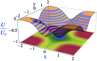
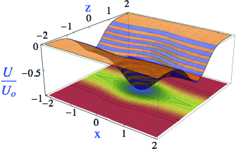
Figure 1: Upper panel: Interaction potential $u(x,y,z)$ along the $z=0$ plane. Lower panel: Interaction potential $u(x,y,z)$ along the $y=0$ plane. Dimensionless coordinates $(x=X/\omega_{o},y=Y/\omega_{o},z=Z/\omega_{o})$ are used.

The classical Hamiltonian describing the motion of an atom of mass $m$ in this cross-beam trap is given by

$${\cal H}=\frac{P_{X}^{2}+P_{Y}^{2}+P_{Z}^{2}}{2m}+U(X,Y,Z),$$ ((4))

where $V_{i}=P_{i}/m$, $i=X,Y,Z$, are the Cartesian components of the velocity of the atom. For this study, it is useful to introduce a dimensionless version of the Hamiltonian (4). To do so, we define the dimensionless coordinates $x=X/w_{o}$, $y=Y/w_{o}$ and $z=Z/w_{o}$ and the dimensionless unit of time $t^{\prime}=t\ \nu$ with the frequency $\nu=(U_{o}/w_{o}^{2}m)^{1/2}$. Applying these transformations to the Hamiltonian (4), we get the following dimensionless Hamiltonian

$$E={\cal H}=\frac{v_{x}^{2}+v_{y}^{2}+v_{z}^{2}}{2}+u(x,y,z),$$ ((5))

where $v_{i}=dx_{i}/dt$ are the corresponding velocity components of the atom and the (dimensionless) dipole potential $u(x,y,z)$ takes the form

$$u(x,y,z)= - \frac{1}{2}\exp\left[-2\,(y^{2}+z^{2})\right]$$

$$- \frac{1}{2}\exp\left[-2\,(x^{2}+z^{2})\right].$$

The coordinates and the energy $E$ are given in units of $w_{o}$ and $U_{o}$, respectively. Thence, the energy of the dipole trap at its minimum is $-1$ and its effective depth is $-1/2$ (see Fig. 1).

The classical equations of motion read

$$\dot{x} = v_{x},\qquad\dot{y}=v_{y},\qquad\dot{z}=v_{z},$$

$$\dot{v}_{x} = -2\ x\ \exp\left[-2(x^{2}+z^{2})\right],$$ ((7))

$$\dot{v}_{y} = -2\ y\ \exp\left[-2(y^{2}+z^{2})\right],$$

$$\dot{v}_{z} = -2\ z\ \left\{\exp\left[-2(y^{2}+z^{2})\right]+\exp\left[-2(x^{2}+z^{2})\right]\right\}.$$

In this system of coupled equations, there are three families of periodic orbits. The rectilinear orbits, $I_{x}$, $I_{y}$ and $I_{z}$, along the $x$, $y$ and $z$ axes, which are always particular solutions of Sec. II. Orbits $I_{x}$ and $I_{y}$ are plotted in Fig. 2. For $z=v_{z}=0$, we find the rectilinear orbits, $I_{xy}^{\pm}$, with initial conditions $x=\pm y$ and $v_{x}=\pm v_{y}$, i. e., the two bisectors of the $xy$ plane, and the elliptic-shaped trajectories, $I_{E}^{\pm}$, for the initial conditions $x=\pm y$ and $v_{x}=\mp v_{y}$ (see Fig. 2).

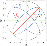
Figure 2: Examples of the periodic orbits $I_{x}$, $I_{y}$, $I_{xy}^{+}$, $I_{xy}^{-}$, $I_{E}^{+}$ and $I_{E}^{-}$ in the $xy$-plane for the energy $E=-0.9$.

In the invariant plane $z=v_{z}=0$, i. e., the trajectories with initial conditions $z(0)=v_{z}(0)=0$ always satisfy $z(t)=v_{z}(t)=0$. The degrees of freedom $(x,v_{x})$ and $(y,v_{y})$ are decoupled in the Hamiltonian ((5)) and the system is integrable. There are two more invariant planes given by $x=v_{x}=0$ and $y=v_{y}=0$ which present an equivalent dynamics with two degrees of freedom due to the symmetry between the coordinates $x$ and $y$, and between their corresponding velocities. If the motion of the atom is confined close to the trap minimum, the dipole potential (II) could be approximated by the harmonic one $U(x,y,z)\approx x^{2}+y^{2}+2z^{2}-1$, and the system becomes a harmonic oscillator in 3D which is integrable and separable.

III Nonlinear Dynamics of the trapped atom

Here, we focus on the phase space structure of an atom confined in the optical dipole trap governed by the Hamiltonian (5). The latter involves three degrees of freedom, and the corresponding phase space is six-dimensional leading to a five-dimensional energy shell. Thus, Poincaré surfaces of section poincare ; poincare1 are not useful to investigate the phase space structures. The so-called chaos indicators represent an alternative to perform such a study barrio ; barrio1 . One of the most popular is the Orthogonal Fast Lyapunov indicator (OFLI) ofli1 ; ofli2 ; ofli22 , defined as

$$\mbox{OFLI}({\bf r}_{0},\delta{\bf r}_{0},t_{f})=\sup_{0\leq t\leq t_{f}}\log||\delta{\bf r}^{\bot}(t)||$$ ((8))

where ${\bf r}(t)=(x(t),y(t),z(t))$, ${\bf r}_{o}={\bf r}(0)$, $\delta{\bf r}^{\bot}$ is the component of the variational vector $\delta{\bf y}$ orthogonal to the flow $d{\bf r}/dt$, and $t_{f}$ is the stopping time. The OFLI provides a fast way to determine if an orbit is chaotic and is able to distinguish between periodic and resonant orbits. In this way, the variational vector $\delta{\bf r}^{\bot}$ behaves linearly for regular resonant orbits and for orbits on a KAM torus; it tends to constant values for periodic ones, and it increases exponentially for chaotic ones ofli2 ; ofli22 ; ofli3 . Examples of this behavior are shown in Fig. 4 and Fig. 5.2 of references barrio and ofli33 , respectively. Note that the Lyapunov exponents are defined in the long-time limit (see e.g. Ref. friedrich ), in contrast to the OFLI definition ((8)). The main disadvantage is that the OFLI results depend on the initial conditions of the variational vector $\delta{\bf y}_{o}$. Here, we use the so-called OFLI${}^{TT}_{2}$ extension of OFLI barrio ; barrio1 , which removes the drawback of choosing $\delta{\bf y}_{o}$ by incorporating the second order variational equations in the computation of the indicator.

In the six-dimensional system ((5)), a two-dimensional OFLI${}^{TT}_{2}$ map is obtained by imposing three restrictions in addition of fixing the energy $E$. To implement the latter, we have to choose two proper two-dimensional subspaces of initial conditions. Since the $x$ and $y$ coordinates are dynamically equivalent, we choose the two planar subspaces ${\cal S}_{1}=\left\{(y,z),x=v_{y}=v_{z}=0\right\}$ and ${\cal S}_{2}=\left\{(x,y),z=v_{x}=v_{y}=0\right\}$, which are perpendicular to the $x$ and $z$-axes, respectively. For a fixed energy $E$, the energy condition ((5)) provides the initial value for the velocities

$$v_{x} = \pm\sqrt{2E+\exp[-2(y^{2}+z^{2})]+\exp[-2z^{2}]},$$ ((9))

$$v_{z} = \pm\sqrt{2E+\exp[-2x^{2}]+\exp[-2y^{2}]},$$ ((10))

in ${\cal S}_{1}$ and ${\cal S}_{2}$, respectively. For $v_{x}=0$ and $v_{z}=0$, these equations give the available regions $(y,z)$ and $(x,y)$ in the planar subspaces ${\cal S}_{1}$ and ${\cal S}_{2}$, respectively.

We have calculated the OFLI${}^{TT}_{2}$ by the numerical integration of the Hamiltonian equations of motion II using an explicit Runge-Kutta algorithm of eighth order with step size control and dense output Hairer . In our calculations, we stop the time evolution, if the OFLI${}^{TT}_{2}$ reaches the value nine that characterizes a chaotic orbit or if $t$ becomes larger than the stopping time $t_{f}=2000$. Our numerical tests have shown that this value for the stopping time is appropriate for the correct characterization of any orbit. In Fig. 3 we present the short and the long time evolution of the OFLI${}^{TT}_{2}$ for a quasiperiodic and a chaotic trajectories and for the periodic orbit $I_{z}$. The energy of these orbits is $E=-0.6$ and their initial conditions have been taken from the OFLI${}^{TT}_{2}$ map of Fig. 5 b. These time evolutions show that with a stopping time of $t_{f}=2000$ the main features of these orbits are correctly captured.

 

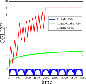
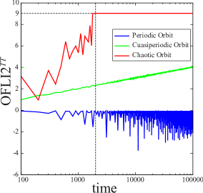
Figure 3: Sort (left panel) and long (right panel) time evolution of the OFLI${}^{TT}_{2}$ indicator for a quasiperiodic and a chaotic trajectories and for the periodic orbit $I_{z}$. Note that in the right panel a logarithmic scale has been used for the abscissa axis. Their energy is $E=-0.6$ and their initial conditions have been taken from the OFLI${}^{TT}_{2}$ map of Fig.5 b. The vertical and horizontal dashed lines indicate the stopping time $t_{f}=2000$ and the cut-off value nine of the OFLI${}^{TT}_{2}$ for chaotic orbits, respectively.

In the OFLI${}^{TT}_{2}$ maps, we have used a RGB (Red Green Blue) color code: blue and red are associated to regular and chaotic orbits, respectively; intermediate colors from dark blue to red indicate the evolution from regular to chaotic motion; finally pink and white stand for not allowed initial conditions and escape orbits, respectively.

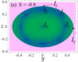
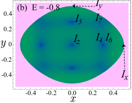
Figure 4: OFLI${}^{TT}_{2}$ indicator color maps for initial conditions in the plane ${\cal S}_{1}=\left\{(y,z),x=v_{y}=v_{z}=0\right\}$ (upper panel) and in the plane ${\cal S}_{2}=\left\{(x,y),z=v_{x}=v_{y}=0\right\}$ (lower panel) and energy $E=-0.8$. The pink color stands for energetically not allowed initial conditions.

If the energy of the atom is close to the potential well minimum, the phase space is populated with highly regular orbits having small OFLI${}^{TT}_{2}$ values. This is illustrated in Fig. 4 by the OFLI${}^{TT}_{2}$ maps for $E=-0.8$. The dark-blue points in these maps correspond to several stable periodic orbits surrounded by a set of KAM tori. The positions of the analytical periodic orbits $I_{x}$, $I_{y}$ and $I_{z}$ are shown. For these OFLI${}^{TT}_{2}$ maps, we have computed seven non-trivial periodic orbits, $I_{i},\ i=1,\dots,7$, which are indicated in the corresponding panel of Fig. 4. They are also listed in Table 1 with the resonance order $m:n:k$, which means that $w_{x}/w_{y}=m/n$ and $w_{y}/w_{z}=n/k$, with $w_{x}$, $w_{y}$ and $w_{z}$ being the frequencies of each mode, and $m,n$, and $k$ integers.

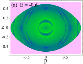
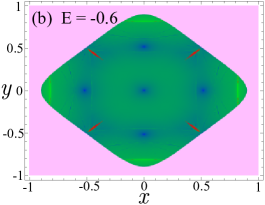
Figure 5: Same as Fig.4 but for energy $E=-0.6$.

For $E=-0.6$, the phase space still presents a predominantly regular behavior, see Fig. 5. Compared to the $E=-0.8$ case, the OFLI${}^{TT}_{2}$ maps are dominated by a lighter green color due to the existence of quasiperiodic orbits with larger values of OFLI${}^{TT}_{2}$. The evolution of the OFLI${}^{TT}_{2}$ along the $z=0$ and $y=0$ axes is presented in Fig. 6 (a) and Fig. 6 (b), respectively. These one-dimensional plots clearly show that larger values of OFLI${}^{TT}_{2}$ are achieved for $E=-0.6$. Moreover, we observe along the $z=0$ axis the major impact of the presence of the periodic orbits $I_{x}$, $I_{y}$ and $I_{1}$ (see Table 1). In Fig. 6 (b), we detect the OFLI${}^{TT}_{2}$ signature of the $I_{x}$, $I_{z}$, $I_{4}$ and $I_{6}$ periodic orbits (see Table 1). For $E=-0.6$, Fig. 6 (b) shows the presence of three new periodic orbits (resonances), namely $I_{8}$ (2:0:1), $I_{9}$ (5:0:3) and $I_{10}$ (11:0:7), which are also depicted in Table 1. The dynamics is more complex for $E=-0.6$. For instance, the inset of Fig. 6 (b) shows that the periodic orbit $I_{9}$ is embedded between two quasiperiodic orbits with high values of OFLI${}^{TT}_{2}$. The phase space in Fig. 5 (b) presents small regions of chaotic motion (in red) along the direction $x=\pm y$, in which OFLI${}^{TT}_{2}$ surpasses the chaotic limit during its evolution, cf. Fig. 6 (c). Obviously, for $E<-0.5$, all orbits are bounded.

Name	Projections	Resonance	Name	Projections	Resonance
Type		$m:n:k$	Type		$m:n:k$
$I_{1}$ 2D		1:1:0	$I_{2}$ 2D		10:0:7
$I_{3}$ 3D		10:10:7	$I_{4}$ 2D		13:0:9
$I_{5}$ 2D		0:26:17	$I_{6}$ 2D		10:0:7
$I_{7}$ 3D		7:7:5	$I_{8}$ 2D		2:0:1
$I_{9}$ 2D		5:0:3	$I_{10}$ 2D		11:0:7

Table 1: Main non-trivial periodic orbits appearing in the OFLI${}^{TT}_{2}$ maps in Fig.4. These orbits are illustrated by using the projections on the $zx$ or $yx$ planes. We provide the $m:n:k$ order of the resonance. The blue and red orbits correspond to the energies $E=-0.8$ and $E=-0.6$, respectively.

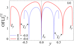
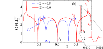
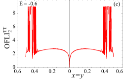
Figure 6: Evolution of the OFLI${}^{TT}_{2}$ indicator along: (a) the $z=0$ direction ($x=p_{y}=p_{z}=0$) for energies $E=-0.8$ (blue dashed line) and $E=-0.6$ (red solid line); (b) the $y=0$ direction ($z=p_{x}=p_{y}=0$) for $E=-0.8$ (blue dashed line) and $E=-0.6$ (red solid line); (c) the $x=y$ direction ($z=p_{x}=p_{y}=0$) for $E=-0.6$.

For $E>-0.5$, the $x$ and $y$ directions become escape channels by which the atoms could leave the optical trap. Thus, the available region of the OFLI${}^{TT}_{2}$ map in the planar subspaces ${\cal S}_{1}$ and ${\cal S}_{2}$ are open along the $x$ and $y$ axes, respectively; whereas the channel along $z$ remains closed for negative energies. Due to these escape channels, the computation of the OFLI${}^{TT}_{2}$ indicator is stopped if, for $t<t_{f}$, the distance of the atom from the trap center reaches a certain fixed threshold $r_{t}=5$.

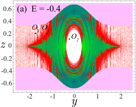
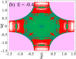
Figure 7: Same as Fig.4 but for energy $E=-0.4$.

For $E=-0.4$, the dynamics is more complex and the phase space is a mixture of chaotic and regular motion around KAM tori, see Fig. 7. Note that the initial conditions in the wide red regions of Fig. 7 give rise to chaotic orbits (in a non-strict sense) that after being trapped for some time finally escape footnote_mia . These orbits have a transient chaotic regime while the atom remains confined in the trap. Once the atom leaves the trap through one of the escape channels, it becomes a free particle and its regular motion is not affected by the potential well. In many cases, the elapsed time before the atom leaves the trap is much larger than the stopping time $t_{f}=2000$ used in this work. This is illustrated in Fig. 8 with the evolution of the escape time of chaotic orbits in Fig. 7(a) along the $z=0.2$ direction for $E=-0.4$. It is important to note that the stopping time used in the computation of Fig. 8 is $t_{f}=10^{6}$.

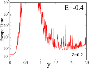
Figure 8: Evolution of the escape time of the chaotic orbits in Fig. 7 (a) along the $z=0.2$ direction for $E=-0.4$. The stopping time used to obtain these chaotic orbits is $t_{f}=10^{6}$.

For more than two-degree of freedom, KAM tori do not partition phase space. As a consequence, and due to diffusion through the Arnold’s web arnold , chaotic orbits can explore all the phase space regions not occupied by the bounded KAM orbits, in such a way that, sooner or later, the atoms leave the trap. As an example, we show in Fig. 9 (a) the long-lived escape chaotic orbit $O_{1}$ with initial conditions in Fig. 7 (a). In the maps of Fig. 7 the white zones correspond to initial conditions of orbits that escape “quickly” from the trap, i. e., the elapsed time when the atom leaves the trap is much smaller than $t_{f}$. Actually, these quick escape orbits have a regular behavior. In the white central region of the OFLI${}^{TT}_{2}$ maps in Fig. 7 (a), the regular trajectories escape along the $x$-axis, such as, e. g., the orbit $O_{2}$ plotted in Fig. 9 (b). Whereas, in the regular white areas surrounded by chaotic motion in the left and right sides of Fig. 7 (a), the atoms quickly leave the trap along the $y$ axis, e. g., the orbit $O_{3}$ depicted in Fig. 9 (c). The central region of the OFLI${}^{TT}_{2}$ maps in Fig. 7 (b) corresponds to the region around the $I_{z}$ rectilinear periodic orbit, which has no accessible escape channel for negative energies. In the right and left (upper and lower) white areas embedded between chaotic motion regions in Fig. 7 (b) there are regular trajectories that quickly leave the trap along the $x$ ($y$) -axis, these orbits are similar to those presented in Fig. 9. The orbits with initial conditions in the white regions of Fig. 7 (a) and (b) have confinement times in the trap being very short compared to the orbits within the red regions. It is worth noticing that, for a fixed energy $E$, the size of these white regions do not increase if the integration stopping time $t_{f}$ is increased.

   

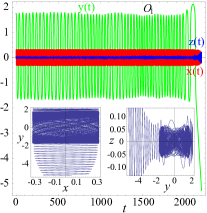
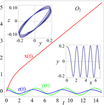
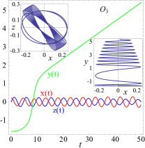
Figure 9: Examples of the time evolution of a chaotic escape orbit ($O_{1}$, left panel) and two regular escape orbits ($O_{2}$ and $O_{3}$, central and right panels). In the insets of the panels are shown the $x-y$ and the $y-z$ projections of each orbit. The three orbits have the same energy $E=-0.4$, and their positions are indicated in Fig. 7 (a).

By further increasing the atomic energy, the size of the central gap increases because the number of orbits having access to the $x$-axis escape channels is enhanced, see Fig. 10 (a), (c) and (e) for $E=-0.3$, $-0.2$ and $-0.1$, respectively. Analogously, the escape regions along the $x$ and $y$ axes become also larger. At the same time, the red chaotic escape regions increase in size whereas the green regular bounded regions shrink, see Fig. 10 (b), (d) and (f). Indeed, bounded regular motion can only be found in small regions entirely surrounded by a chaotic sea. However, even for $E=-0.1$, where most of the orbits are unbounded (whether regular or chaotic), it is still possible to find regions of trapped regular motion.

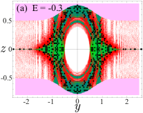
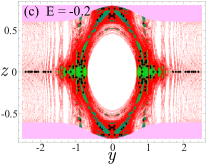
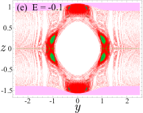
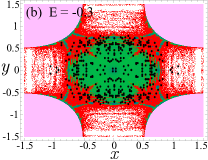
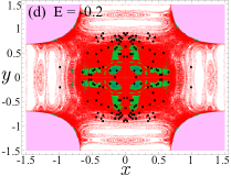
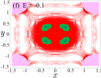
Figure 10: Same as Fig.4 but for energies $E=-0.3$ (a) and (b) panels, $E=-0.2$ (c) and (d) panels and $E=-0.1$ (e) and (f) panels. The black points in panels (a), (b), (c) and (d) indicate the initial conditions of the atomic beam propagating along the $x$ and $z$ axes which are confined when the optical trap is switched on, see Sec. IV for more details.

IV Classical sudden trapping mechanism

In the cold (and ultracold) regime, the availability of confined atomic ensembles provides major advantages as compared to atomic beams. The trapped ensemble allows to perform a wealth of interesting controlled experiments such as high-precision spectroscopy or single atom manipulation PhysRevA.67.033403 . Experimentally, the trapping of atoms requires the manipulation of their collective motion by slowing them down and requires sophisticated techniques for cooling. While the standard procedure of trapping and cooling neutral atoms and ions relies on adiabatic processes, meaning that one first slows or even stops a particle beam before one traps it, we explore here the problem of the trapping of a (finite velocity) beam of particles by a sudden switch on of a trap. Obviously, this is a highly non-adiabatic and instantaneous process but still quite interesting from an experimental point of view. Taking particles suddenly out of an atomic beam is an immediate and straightforward procedure, which would be a simple alternative to the efficient adiabatic trapping because it could be easily implemented in any experiment with cold atoms. Here, we illustrate this sudden trapping mechanism in terms of a classical phase space analysis of the atomic ensemble.

To be specific, we consider an atomic ensemble of $N=1240000$ atoms, initially in free motion, and investigate the trapping features of a crossed optical dipole trap, which is suddenly turned on. Based on the spatial dependence of the optical potential (II), we restrict the atomic ensemble spatial extension to the “prism” ${\cal P}=(-2.5\leq x\leq 2.5,-2.5\leq y\leq 2.5,-1.5\leq z\leq 1.5)$. The initial positions of the atoms are uniformly distributed in this prism ${\cal P}$. We assume that this atomic beam is in thermal equilibrium propagating along the $x$ axis ($v_{y}=v_{z}=0$), with a velocity distribution MetcalfStraten

$$f(v_{x})=\frac{4v_{x}^{3}}{v_{rms}^{4}}\exp(-\frac{2v_{x}^{2}}{v_{rms}^{2}}),$$ ((11))

where $v_{rms}$ is the root mean square beam velocity related to the mean kinetic energy $K_{rms}=v_{rms}^{2}/2$, in reduced units. For a given mean kinetic energy, and using the Monte-Carlo method, an initial positive velocity $v_{x}$ is assigned to each atom according to the velocity distribution ((11)).

Initially the optical trap is off, and the atoms move freely with only kinetic energy $E=v_{x}^{2}/2$. The optical trap is instantaneously switched on at $t=0$, and the free atomic motion is perturbed by the dipole potential. The initial energy $E=v_{x}^{2}/2$ decreases by $u(x,y,z)$, which depends on the atom position. Due to the shape of the potential, atoms around the origin should be strongly perturbed and likely trapped.

The trajectories of the atoms are computed by integrating numerically the Hamiltonian equations of motion (II). If after a convenient propagation cut-off time $t_{c}$, fixed here to $t_{c}=2\times 10^{4}$, the distance of an atom from the trap center is still below the threshold distance $r_{t}=5$, we consider that the atom is trapped. To choose $t_{c}$, we have taken into account that for $E>-0.5$, the chaotic orbits are always escape orbits, see the previous section, with an elapsed time before leaving the trap being extremely long in many cases, i. e., the diffusion is extremely slow compared to the trapping time. For instance, in a typical dipole trap for Rb atoms with beam waist $\omega_{o}=25\ \mu$m and well depth $U_{o}=1.5$ mK wieman , the frequency and time units are $\nu=(U_{o}/w_{o}^{2}m)^{1/2}\approx 1.5\times 10^{4}$ s^-1 and $t\approx 1/1.5\times 10^{-4}$ s, respectively. Since in a conventional experiment, the trap is filled in a few seconds, the cut-of time value $t_{c}=2\times 10^{4}$ seems to be appropriate. Note that we are assuming as trapped orbits the chaotic ones whose escape time is above $t_{c}=2\times 10^{4}$.

For three mean kinetic energies $K_{rms}$ of the atomic beam, we present in Fig. 11 the energy distribution histograms of the trapped orbits, indicating the number of trapped atoms $N_{trapped}$ and the ratio $n$ between the number of trapped atoms with energy larger than the threshold energy ($E>-0.5$) and $N_{trapped}$. As it should be expected, by increasing the initial mean kinetic energy $K_{rms}$ the amount of trapped atoms $N_{trapped}$ decreases. For the fast beam with $K_{rms}=0.5$, only $1.4\%$ of the initial atoms remain trapped. However, the majority of these atoms have an energy larger than the escape channels, indeed, $n$ is always larger than $0.65$, i. e., for more than $65\%$ of the trapped atoms, $E>-0.5$. This is also observed in the large tail of the histograms in Fig.11.

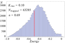
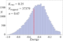
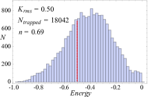
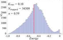
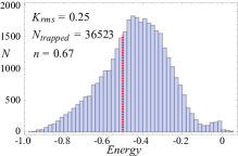
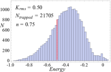
Figure 11: Energy distribution histograms of the trapped orbits for three different mean kinetic energies $K_{rms}$ of the atomic beam. $N_{trapped}$ is the number of trapped atoms and $n$ is the ratio of the number of trapped atoms with energy greater than $E=-0.5$ and $N_{trapped}$. Upper and lower row histograms correspond to the case of the atomic beam propagating along the $x$ and $z$ axes, respectively.

Now, we compare the trapping ability of the optical trap for atomic beams propagating along the $x$ and $z$ directions. We consider that the atoms move in the $z$ axis with velocity $v_{z}$ given by the distribution ((11)) and $v_{x}=v_{y}=0$. The corresponding results are presented in the histograms of the lower panels in Fig. 11, where we observe quantitatively similar results. As $K_{rms}$ is increased, $N_{trapped}$ decreases whereas $n$ increases. In particular, for $K_{rms}=0.10$ and $0.5$, the percentage of trapped atoms with $E>-0.5$ are $59\%$ and $75\%$, respectively. Hence, we can conclude that the trapping ability of the optical trap is very similar for an atomic beam propagating along the $z$ and $x$ axes.

The explanation of why such a large amount of atoms with $E>-0.5$ remains trapped can be found in the OFLI${}^{TT}_{2}$ maps. In the $E=-0.3$ OFLI${}^{TT}_{2}$ maps of Fig. 10 (a) and (b), the black points indicate the initial conditions of the atomic beam propagating along the $x$ and $z$ axes, respectively, which are confined when the optical trap is switched on. In both cases, most of the black points lay on green regions of bounded regular motion. Thus, after switching on the lasers, the confined atoms with energy $E>-0.5$ are in phase space regions where bounded motion is still possible due to the existence of persistent KAM tori. Indeed, these dynamical structures are responsible for the capture of atoms with an energy larger than the trapping energy threshold. There are also many black points in red chaotic regions, which are escape chaotic orbits that remain trapped for long periods of time. For $E=-0.2$, the initial conditions of the confined orbits are also plotted in Fig. 10 (c) and (d). In this case, most of the bounded trajectories are confined in chaotic regions because the regular KAM tori regions have shrunken.

V Conclusions

We have investigated the nonlinear dynamics of an atom in a crossed optical dipole trap formed by two identical Gaussian laser beams propagating along perpendicular directions. The evolution of the stability of the dynamics with increasing energy has been shown by a detailed analysis of the phase space in terms of two dimensional OFLI${}^{TT}_{2}$ maps. For small energies, the phase space is populated with periodic and quasi periodic orbits, but chaotic motion appears as the energy is increased. Above a certain threshold, escape in both spatial ($x$, $y$) degrees of freedom becomes possible and the dynamics is of mixed regular and chaotic character. Regular trajectories in which the atom quickly leaves the trap, and chaotic ones with very long escape times exist in this case. For energies close to zero, the threshold for escape in all three spatial directions, the phase space still presents small areas of trapped regular motion which are surrounded by a sea of chaotic scattering ott .

Furthermore, we have explored the impact of an optical dipole trap, which is suddenly turned on, on an atomic beam that moves freely. Independently of the initial direction of the atoms, we encounter that some of them remain within the trap, and the amount of trapped atoms decreases, as expected, as the initial atomic energy is increased. The majority of these trapped atoms have an energy larger than the escape channels, which can be understood in terms of the phase space structures. The OFLI${}^{TT}_{2}$ maps show that these trapped atoms are either in bounded orbits, which are possible due to the existence of KAM tori, or in chaotic ones with very long escape times.

A natural extension of this work would be to investigate the dynamics following a quench. For an atomic ensemble in an optical dipole trap, a sudden change of the trap depth or width would provoke significant changes in the phase space structure. A classical study based on OFLI${}^{TT}_{2}$ maps would then characterize the escape dynamics and trapped population.

- (1) A. Ashkin, Phys. Rev. Lett. 24, 156 (1970).
- (2) A. Ashkin, Phys. Rev. Lett. 40, 729 (1978); J. E. Bjorkholm, R. R. Freeman, A. Ashkin and D. B. Pearson, Phys. Rev. Lett. 41, 1361 (1978).
- (3) S. Chu, J. E. Bjorkholm, A. Ashkin and A. Cable, Phys. Rev. Lett. 57 314 (1986).
- (4) R. Grimm, M. Weidemüller and Y. B. Ovchinnikov, Adv. At. Mol. and Opt. Phys., 42, 95 (2000).
- (5) H. J. Metcalf and P. van der Straten, Laser Cooling and Trapping (Springer-Verlag, New York, 1999).
- (6) W. Alt, D. Schrader, S. Kuhr, M. Müller, V. Gomer, and D. Meschede, Phys. Rev. A 67, 033403 (2003).
- (7) M. H. Anderson, J. R. Ensher, M. R. Matthews, C. E. Wieman, and E. A. Cornell Science 269, 198 (1995); K. B. Davis, M. -O. Mewes, M. R. Andrews, N. J. van Druten, D. S. Durfee, D. M. Kurn, and W. Ketterle, Phys. Rev. Lett. 75, 3969 (1995); C. C. Bradley, C. A. Sackett, and R. G. Hulet, Phys. Rev. Lett. 78, 985 (1997).
- (8) N. Poli, C. W. Oates , P. Gill and G. M. Tino, Rivista del Nuovo Cimento 36, 555 (2013).
- (9) V. Milner, J. L. Hanssen, W.C. Campbell and M. G. Raizen, Phys. Rev. Lett. 86, 1514 (2001).
- (10) N. Friedman, A. Kaplan, D. Carasso and N. Davidson, Phys. Rev. Lett. 86, 1518 (2001).
- (11) C. S. Adams, H. J. Lee, N. Davidson, M. Kasevich and S. Chu, Phys. Rev. Lett. 74, 3577 (1995).
- (12) R. Fulton, A. I. Bishop, and P. F. Barker, Phys. Rev. Lett. 93, 243004 (2004); S. M. Purcell and P. F. Barker, Phys. Rev. A 82, 033433 (2010).
- (13) P. S. Pershan, J. P. van der Ziel and L. D. Malmstrom, Phys. Rev. 143, 574 (1966).
- (14) H. Poincaré, Les Méthodes Nouvelles de la Mécanique Céleste (Gauthiers-Villars, 1892).
- (15) A. J. Lichtenberg and M. A. Lieberman, Regular and Chaotic Dynamics (Springer-Verlag, New York, 1992)
- (16) R. Barrio, Chaos, Solitons and Fractals 25, 711 (2005).
- (17) R. Barrio, Int. J. Bif. and Chaos 16, 2777 (2006).
- (18) C. Froeschlé, E. Lega and R. Gonczi, Celes. Mech. Dyn. Astr. 67, 41 (1997).
- (19) C. Froeschlé and E. Lega, Celes. Mech. Dyn. Astr. 78, 167 (2000).
- (20) M. Fouchard, E. Lega and C. Froeschlé, Celes. Mech. Dyn. Astr. 83, 205 (2002).
- (21) C. Froeschlé and E. Lega, Astr. Astrophys. 334, 355 (1998).
- (22) C. Froeschlé and E. Lega, Hamiltonian Systems and Fourier Analysis: New Prospects for Gravitational Dynamics (Advances in Astronomy & Astrophysics,Cambridge Scientific Publishers, Cambridge, 2005).
- (23) H. Friedrich, Theoretical Atomic Physics (Springer-Verlag, Berlin, 2006).
- (24) S. N. E. Hairer and G. Wanner, Solving Ordinary Differential Equations I. Nonstiff Problems (Springer Series in Computational Mathematics, Springer-Verlag, New York, 1993).
- (25) Strictly speaking, an orbit is chaotic if its largest Lyapunov exponent is positive, which implies a sensitive dependence on initial conditions. A chaotic orbit in a close system is characterized by the finiteness of the Liapunov exponent, as a consequence of which the exponential sensitivity has its trace at all phases of the chaotic orbits (we exclude here, for simplicity, the case of stickiness to regular islands). In contrast, for the chaotic scattering in an open system, there is an asymptotic ballistic motion, that is distinguished from the chaotic behavior in a closed system.
- (26) V. I. Arnold, Russ. Math. Surv. 18, 9 (1963).
- (27) S. J. M. Kuppens, K. L. Corwin, K. W. Miller, T. E. Chupp, and C. E. Wieman, Phys. Rev. A 62, 013406 (2000).
- (28) E. Ott and T. Tél. Chaos 3, 417 (1993).