Continuous representation for shell models of turbulence

Abstract

In this work we construct and analyze continuous hydrodynamic models in one space dimension, which are induced by shell models of turbulence. After Fourier transformation, such continuous models split into an infinite number of uncoupled subsystems, which are all identical to the same shell model. The two shell models, which allow such a construction, are considered: the dyadic (Desnyansky–Novikov) model with the intershell ratio $\lambda=2^{3/2}$ and the Sabra model of turbulence with $\lambda=\sqrt{2+\sqrt{5}}\approx 2.058$. The continuous models allow understanding various properties of shell model solutions and provide their interpretation in physical space. We show that the asymptotic solutions of the dyadic model with Kolmogorov scaling correspond to the shocks (discontinuities) for the induced continuous solutions in physical space, and the finite-time blowup together with its viscous regularization follow the scenario similar to the Burgers equation. For the Sabra model, we provide the physical space representation for blowup solutions and intermittent turbulent dynamics.

1 Introduction

Shell models represent simplified “toy” models demonstrating various nontrivial phenomena of developed hydrodynamic turbulence, many of which are still not fully understood [11, 3]. These models consider a geometric series of wavenumbers, $k_{n}=k_{0}\lambda^{n}$ with $n\in\mathbb{Z}$ and fixed $\lambda>1$. Each shell is represented by one or several (real or complex) numbers called shell speeds, which mimic the velocity field at a given scale $\delta r\sim 2\pi/k_{n}$. The evolution of shell speeds is governed by infinite-dimensional systems of ordinary differential equations, which allow for local interaction among the shells and must share several properties like scaling invariance, quadratic nonlinearity, energy conservation etc. with the Navier-Stokes equations or other hydrodynamic models. Originating in early 70s, see e.g. [16, 13, 9], shell models became especially popular with the construction of the Gledzer–Ohkitani–Yamada (GOY) model [13, 25], which has the chaotic intermittent dynamics in the inertial interval with the statistical properties close to the Navier-Stokes developed turbulence. In this paper, we consider the following shell models: the dyadic (Desnyansky–Novikov) model [9] and the Sabra model of turbulence [17] representing a modified version of the GOY model.

The derivation of shell models is usually based of restricting the Fourier transformed hydrodynamic equations to a very limited number of modes (shells). Such simplification leads to a strongly reduced system, so that the same shell model can be derived from different original systems, e.g., Burgers or Navier-Stockes equations [26, 21]. As a result, shell model solutions generally lose their quantitative relation with the original systems, though they may retain some important qualitative properties. This leads to the problem of interpreting the results obtained for shell models in their relation with the continuous solutions in physical space.

In this paper, we construct one-dimensional continuous hydrodynamic models, from which the shell models can be derived without any simplifications, i.e., in a rigorous way. This means that the Fourier transformed continuous models split into an infinite set of uncoupled subsystem, where each subsystem is equivalent to the same shell model under consideration. Such continuous models are characterized by nonlocal quadratic nonlinearity (similarly to the nonlocal term induced by pressure in incompressible flows), conserve energy and may have some other properties like the Hamiltonian structure etc. This construction is carried out for the two cases: the dyadic model with the intershell ratio $\lambda=2^{3/2}$ and the Sabra model with $\lambda=\sqrt{2+\sqrt{5}}\approx 2.058$. Note that our approach uses the fixed values of $\lambda$, as opposed to the limiting models obtained as $\lambda\to 1$ [1].

The proposed continuous models resolve the problem of representing the shell model solutions in physical space. This allows interpreting various results for shell models by relating them with the known properties of continuous flows or, more generally, of evolutionary partial differential equations. We demonstrate this by showing that the asymptotic solution with the Kolmogorov scaling, $u_{n}\propto k_{n}^{-1/3}$, in the dyadic shell model corresponds to a shock (discontinuity) for the induced continuous solution in physical space. Furthermore, the finite-time blowup together with its viscous regularization in the dyadic model follow the scenario similar to the Burgers equation for the continuous representation. Another implication of this approach is the physical space representation of intermittent turbulent dynamics in the Sabra model.

The paper is organized as follows. Section 2 describes the properties of one-dimensional hydrodynamic models. Section 3 analyzes the continuous representation of the dyadic (Desnyansky–Novikov) shell model, and Section 4 does the same for the Sabra model of turbulence. We finish with some conclusions.

2 One-dimensional hydrodynamic models

We consider one-dimensional models for a scalar variable $u(x,t)$ in the form

$$\frac{\partial u}{\partial t}+\frac{\partial g}{\partial x}=\nu\frac{\partial^{2}u}{\partial x^{2}}+f,\quad x,t\in\mathbb{R},$$ (2.1)

where $\nu$ is a viscous coefficient, $f(x,t)$ is the forcing term and

$$g(x,t)=\frac{1}{2\pi}\iint K(y-x,z-x)u(y,t)u(z,t)dydz$$ (2.2)

is the nonlocal quadratic flux term. For hydrodynamic models, where the quadratic term originates from the convective acceleration (and pressure for inviscid flows), it is natural to assume that $K(y,z)$ is a real homogeneous function of degree $-2$. Therefore, it can be considered in the form

$$K(y,z)=\iint\varphi\left(\frac{p}{p+q}\right)e^{-i(py+qz)}dpdq,$$ (2.3)

with a real function $\varphi(\xi)$. For example, the product of Dirac delta functions $K(y,z)=\pi\delta(y)\delta(z)$ corresponds to $\varphi\equiv(4\pi)^{-1}$ and generates the Burgers equation with $g=u^{2}/2$ in Eq. (2.1).

We do not specify the functional spaces for solutions $u(x,t)$ and for the kernel $K(y,z)$, assuming that they allow the integral (Fourier) transformations used below. We will comment on this issue when considering a specific form of $K(y,z)$ in the next section. It is clear that the function $K(y,z)$ in Eq. (2.2) can always be chosen symmetric, i.e., $K(y,z)=K(z,y)$. One can check that permuting the variables $y\leftrightarrow z$ in the expression (2.3) is equivalent to permuting $p\leftrightarrow q$ and substituting $\varphi(\xi)$ by $\varphi(1-\xi)$. Thus, the symmetry of $K(y,z)$ is equivalent to the condition

$$\varphi(\xi)=\varphi(1-\xi),$$ (2.4)

which will be assumed from now on.

For the Fourier transformed function $u(k)=\int u(x)e^{-ikx}dx$, Eqs. (2.1)–(2.3) reduce to

$$\frac{\partial u(k)}{\partial t}=-ik\int\varphi\left(\frac{p}{k}\right)u(p)u(k-p)dp-\nu|k|^{2\alpha}u(k)+f(k),$$ (2.5)

where we omitted the argument $t$ for simplicity of notations. We also introduced the parameter $\alpha$, such that $\alpha=1$ corresponds to Eq. (2.1) and $\alpha>1$ determines the model with hyperviscosity. The mean value $\int u(x)dx$ is conserved by Eq. (2.1) provided that $\int f(x)dx=0$ and $g\to 0$, $\partial u/\partial x\to 0$ as $|x|\to\infty$. We will assume the vanishing mean values, leading to $f(k)=u(k)=0$ for $k=0$. Recall the reality condition $u(-k)=u^{*}(k)$ for the Fourier transformed real function, where the asterisk denotes the complex conjugation.

2.1 Energy conservation

We define the energy as

$$E=\frac{1}{2}\int u^{2}(x)dx=\frac{1}{4\pi}\int|u(k)|^{2}dk.$$ (2.6)

Let us show that the energy conservation condition in the inviscid model with zero force ($\nu=f=0$) is given by the equality

$$\varphi\left(\xi\right)-\xi\varphi\left(\frac{1}{\xi}\right)+(\xi-1)\varphi\left(\frac{1}{1-\xi}\right)=0$$ (2.7)

for all $\xi\in\mathbb{R}$. Indeed, using the reality condition $u^{*}(k)=u(-k)$ and $\nu=f=0$ in Eqs. (2.5), (2.6), we have

$$\frac{dE}{dt}=\frac{1}{2\pi}\mathrm{Re}\int u^{*}(k)\frac{\partial u(k)}{\partial t}dk=\frac{1}{2\pi}\mathrm{Im}\iint k\varphi\left(\frac{p}{k}\right)u(-k)u(p)u(k-p)dpdk.$$ (2.8)

By introducing $q=k-p$ and changing sign of $k$, we can write this expression as

$$\frac{\partial E}{\partial t}=-\frac{1}{2\pi}\mathrm{Im}\iiint k\varphi\left(-\frac{p}{k}\right)\delta(k+p+q)u(k)u(p)u(q)dkdpdq.$$ (2.9)

Due to the symmetry of the factor $u(k)u(p)u(q)$ with respect to permutations of variables $(k,p,q)$, this expression vanishes for an arbitrary function $u(k)$ if

$$k\left[\varphi\left(-\frac{p}{k}\right)+\varphi\left(-\frac{q}{k}\right)\right]+p\left[\varphi\left(-\frac{k}{p}\right)+\varphi\left(-\frac{q}{p}\right)\right]+q\left[\varphi\left(-\frac{k}{q}\right)+\varphi\left(-\frac{p}{q}\right)\right]=0$$ (2.10)

for $k+p+q=0$. Dividing by $k$ and denoting

$$\frac{p}{k}=-\xi,\quad\frac{q}{k}=\frac{-p-k}{k}=\xi-1,\quad\frac{p}{q}=\frac{\xi}{1-\xi},$$ (2.11)

we write (2.10) as

$$\varphi\left(\xi\right)+\varphi\left(1-\xi\right)-\xi\left[\varphi\left(\frac{1}{\xi}\right)+\varphi\left(1-\frac{1}{\xi}\right)\right]+(\xi-1)\left[\varphi\left(\frac{1}{1-\xi}\right)+\varphi\left(\frac{\xi}{\xi-1}\right)\right]=0.$$ (2.12)

This equation reduces to the form (2.7) using the condition (2.4).

In the presence of force, similar derivations yield the equation

$$\frac{dE}{dt}=\int f(x)u(x)dx,$$ (2.13)

where the right-hand side can be interpreted as a work done by the force $f(x)$.

Note that the above derivation of energy conservation implies convergence of all the integrals. Otherwise, the system may dissipate the energy even if the condition (2.7) is satisfied. For example, the condition (2.7) is satisfied for the Burgers equations with $\varphi\equiv(4\pi)^{-1}$, while the shock (weak discontinuous) solutions are dissipative. In this case $u(k)\sim k^{-1}$ for large $k$ and the integral in Eq. (2.8) diverges.

2.2 Hamiltonian structure

Let us show that the condition

$$\varphi\left(\frac{1}{\xi}\right)+\varphi\left(\frac{1}{1-\xi}\right)=2\varphi\left(\xi\right)$$ (2.14)

allows writing Eqs. (2.1)–(2.3) with $\nu=f=0$ in the Hamiltonian form

$$\frac{\partial u}{\partial t}=\{u,H\},$$ (2.15)

where the Hamiltonian and the Poisson bracket are

$$H=\frac{1}{6\pi}\iiint K(y-x,z-x)u(x)u(y)u(z)dxdydz,$$ (2.16)

$$\{F,G\}=-\int\frac{\delta F}{\delta u}\frac{\partial}{\partial x}\frac{\delta G}{\delta u}dx.$$ (2.17)

Here we used the Poisson bracket known for the Korteweg–de Vries (KdV) and inviscid Burgers equations [12, 24]. Note that this Poisson bracket is noncanonical and has the Casimir invariant $C=\int udx$, which we set earlier to zero.

In order to derive Eq. (2.15), we write expression (2.3) in the form

$$K(y-x,z-x)=\iiint\varphi\left(-\frac{p}{k}\right)e^{-i(kx+py+qz)}\delta(k+p+q)dpdqdk,$$ (2.18)

while similar expressions for $K(z-y,x-y)$ and $K(x-z,y-z)$ are obtained after substituting $\varphi\left(-\frac{p}{k}\right)$ by $\varphi\left(-\frac{q}{p}\right)$ and $\varphi\left(-\frac{k}{q}\right)$, respectively. Using these expressions with notations (2.11) and condition (2.4), one can see that Eq. (2.14) implies

$$K(z-y,x-y)+K(x-z,y-z)=2K(y-x,z-x).$$ (2.19)

Then, for $F=u(x^{\prime})$ and $G=H$ from Eq. (2.16), we have

$$\begin{array}[]{rcl}\displaystyle\frac{\delta F}{\delta u(x)}&=&\delta(x-x^{\prime}),\\[12.0pt] \displaystyle\frac{\delta G}{\delta u(x)}&=&\displaystyle\frac{1}{6\pi}\iint\left[K(y-x,z-x)+K(z-y,x-y)+K(x-z,y-z)\right]u(y)u(z)dydz\\[15.0pt] &=&\displaystyle\frac{1}{2\pi}\iint K(y-x,z-x)u(y)u(z)dydz,\end{array}$$ (2.20)

where the last equality follows from Eq. (2.19). Substituting these expressions into Eqs. (2.15), (2.17) yields Eqs. (2.1), (2.2) with $\nu=f=0$.

3 Continuous representation of the Desnyansky–Novikov model

Let us consider the function

$$\varphi(\xi)=\frac{1}{2}\delta\left(\xi-\frac{1}{2}\right)+2\delta(\xi+1)+2\delta(\xi-2),$$ (3.1)

which is the sum of three Dirac delta functions. For the physical space representation of model (2.1), (2.2), we should find the kernel $K(y,z)$ given by Eq. (2.3) with the function (3.1). The integrals in Eq. (2.3) can be taken explicitly using the relation

$$\delta\left(\frac{\xi-\xi_{0}}{a(\xi)}\right)=|a(\xi_{0})|\delta(\xi-\xi_{0}).$$ (3.2)

For the first term, we obtain

$$\begin{array}[]{c}\displaystyle\int\frac{1}{2}\delta\left(\frac{p}{p+q}-\frac{1}{2}\right)e^{-i(py+qz)}dpdq=\int\frac{1}{2}\delta\left(\frac{p-q}{2(p+q)}\right)e^{-i(py+qz)}dpdq\\[15.0pt] \displaystyle=2\int|q|e^{-iq(y+z)}dq=-\frac{4}{(y+z)^{2}},\end{array}$$ (3.3)

where we used that the Fourier transform of $|x|$ is the generalized function $-2k^{-2}=2\frac{d}{dk}\left[\mathrm{p.v.\left(\frac{1}{k}\right)}\right]$, see e.g. [14]. Integrating similarly the other terms in Eqs. (2.3), (3.1), yields

$$K(y,z)=-\frac{4}{(y+z)^{2}}-\frac{4}{(y-2z)^{2}}-\frac{4}{(z-2y)^{2}},$$ (3.4)

and one should consider the singular integrals in Eq. (2.2) with the Hadamard regularization.

The Fourier transformed continuous model has a simpler form. Indeed, substituting $\varphi(\xi)$ from Eq. (3.1) into Eq. (2.5) and using Eq. (3.2) yields

$$\frac{\partial u(k)}{\partial t}=-ik|k|\left[\frac{1}{2}u^{2}\left(\frac{k}{2}\right)+4u^{*}(k)u(2k)\right]-\nu|k|^{2\alpha}u(k)+f(k),$$ (3.5)

where we used the reality condition $u(-k)=u^{*}(k)$. We will show now that this equation is equivalent to an infinite set of uncoupled discrete (shell) models.

Let us define the geometric progression

$$k_{n}=k_{0}\lambda^{n},\quad\lambda=2^{3/2},\quad n\in\mathbb{Z},$$ (3.6)

and the corresponding variables

$$u_{n}=-ik_{n}^{1/3}u\left(k_{n}^{2/3}\right),\quad f_{n}=-ik_{n}^{1/3}f\left(k_{n}^{2/3}\right).$$ (3.7)

Then Eq. (3.5) taken for $k=k_{n}^{2/3}$ reduces to the form

$$\frac{\partial u_{n}}{\partial t}=k_{n}u_{n-1}^{2}-k_{n+1}u_{n}^{*}u_{n+1}-\nu_{n}u_{n}+f_{n},\quad n\in\mathbb{Z},$$ (3.8)

where introduced the viscous factors

$$\nu_{n}=\nu k_{n}^{4\alpha/3}.$$ (3.9)

Equation (3.8) is the shell model, where $k_{n}$ is the shell wavenumber (forming a geometric progression in $n$), $u_{n}\in\mathbb{C}$ is the complex shell speed, and the interaction occurs between the neighboring shells.

One may consider the real variables $u_{n}\in\mathbb{R}$. According to relation (3.7), this is the case when $u(k)$ is a purely imaginary function and, hence, the solution of the continuous model is an odd function in physical space, $u(-x)=-u(x)$. For real variables, system (3.8) becomes

$$\frac{\partial u_{n}}{\partial t}=k_{n}u_{n-1}^{2}-k_{n+1}u_{n}u_{n+1}-\nu_{n}u_{n}+f_{n},\quad n\in\mathbb{Z}.$$ (3.10)

This system is known as the Desnyansky–Novikov (DN) shell model [9], also called the dyadic shell model. Note that, due to the exponent $4\alpha/3$ in this viscous term (3.9), the conventional choice of $\nu_{n}=\nu k_{n}^{2}$ in the shell model corresponds to the continuous model (3.5) with hyperviscosity given by $\alpha=3/2$.

We have shown that the hydrodynamic model given by Eqs. (2.1)–(2.3) and (3.1) splits into a set of equivalent infinite-dimensional subsystems (3.8). Each of these subsystems corresponds to a specific value of the parameter $k_{0}$ in Eq. (3.6), which must be taken in the interval

$$1\leq k_{0}<\lambda.$$ (3.11)

For odd continuous solutions, $u(-x)=-u(x)$, these subsystems take the form of the DN shell model (3.10), where the real variables $u_{n}$ are related to $u(k)$ by Eq. (3.7).

3.1 Energy conservation and Hamiltonian form

Let us consider the shell model (3.8) in the inviscid unforced case, i.e., when $\nu_{n}=f_{n}=0$ for all $n$. Using Eq. (3.2), one can check that the function (3.1) satisfies the conditions

$$\varphi\left(\xi\right)=\varphi\left(1-\xi\right)=\varphi\left(\frac{1}{\xi}\right)=\varphi\left(\frac{1}{1-\xi}\right),$$ (3.12)

which imply the simultaneous energy conservation and Hamiltonian structure, see Eqs. (2.4), (2.7) and (2.14).

Equations (3.6) and (3.7) with $k=k_{n}^{2/3}$ yield

$$u(k)=ik_{n}^{-1/3}u_{n}(k_{0}),\quad k=k_{n}^{2/3}=k_{0}^{2/3}\lambda^{2n/3},$$ (3.13)

$$dk=dk_{n}^{2/3}=\frac{2}{3}\lambda^{2n/3}k_{0}^{-1/3}dk_{0}=\frac{2}{3}k_{n}^{2/3}k_{0}^{-1}dk_{0},$$ (3.14)

where we specified the parameter $k_{0}$ explicitly as an argument for the shell speed $u_{n}$. Using these expressions with the interval (3.11) for $k_{0}$, the energy (2.6) can be written as

$$E=\frac{1}{4\pi}\int\left|u(k)\right|^{2}dk=\frac{1}{4\pi}\int_{0}^{\lambda}\frac{2}{3}k_{0}^{-1}\sum_{n\in\mathbb{Z}}\left|u_{n}(k_{0})\right|^{2}dk_{0}=\frac{1}{6\pi}\int_{0}^{\lambda}k_{0}^{-1}E_{s}(k_{0})dk_{0},$$ (3.15)

where

$$E_{s}(k_{0})=\sum_{n\in\mathbb{Z}}\left|u_{n}(k_{0})\right|^{2}.$$ (3.16)

These expressions relate the energy $E$ of the continuous model with the energies $E_{s}$ of the shell models for all $k_{0}$ from the interval (3.11).

Note that the formal condition of energy conservation was used for derivation of the DN shell model [9]; see also [6, 5, 7] for the detailed analysis in the case of $\lambda=2^{5/2}$. If the initial condition at $t=0$ has finite norm $\sum_{n\in\mathbb{Z}}k_{n}^{2}|u_{n}|^{2}<\infty$, then the inviscid shell model has a unique solution for small times and the energy $E_{s}$ is conserved, see e.g. [8, 22]. However, this norm blows up in finite time leading to dissipative solutions, which we discuss in the next section.

The inviscid unforced continuous model has the Hamiltonian structure given by Eqs. (2.15)–(2.17). This structure induces the corresponding Hamiltonian form for shell model (3.8). The direct derivation of this Hamiltonian form from the continuous formulation is lengthy, and it is easy to find it directly taking into account that the Hamiltonian must be a cubic function of shell speeds $u_{n}$. Indeed, consider the shell model equations written in the canonical form

$$\frac{\partial a_{n}}{\partial t}=-i\frac{\partial H}{\partial a_{n}^{*}}=\frac{1}{2}k_{n}^{4/3}a_{n-1}^{2}-k_{n+1}^{4/3}a_{n}^{*}a_{n+1},$$ (3.17)

where $\{a_{n},a_{n}^{*}\}$, $n\in\mathbb{Z}$, are pairs of complex canonical variables and the real Hamiltonian is given by

$$H=\frac{i}{2}\sum_{n}k_{n}^{4/3}\left(a_{n-1}^{2}a_{n}^{*}-(a^{*}_{n-1})^{2}a_{n}\right).$$ (3.18)

It is easy to see that Eq. (3.17) reduces to Eq. (3.8) with $\nu_{n}=f_{n}=0$ for $a_{n}=k_{n}^{-1/3}u_{n}$, where one should use the relation $k_{n+1}^{2/3}=2k_{n}^{2/3}$ following from Eq. (3.6).

3.2 Shock wave solutions in the inviscid model

Let us consider real solutions of the inviscid DN model (3.10) with the specific constant forcing applied to the shell with $n=0$, i.e.,

$$\frac{\partial u_{n}}{\partial t}=k_{n}u_{n-1}^{2}-k_{n+1}u_{n}u_{n+1}+f_{n},\quad f_{n}=2k_{0}^{1/3}\delta_{n0}.$$ (3.19)

Here $\delta_{n0}$ is the Kronecker delta, which is equal to $1$ for $n=0$ and zero otherwise. We will consider initial conditions in the form

$$t=0:\quad u_{n}=u_{n}^{0}\quad\textrm{for}\quad n\geq 0;\quad u_{n}=0\quad\textrm{for}\quad n<0,$$ (3.20)

assuming no perturbation of the shells with $n<0$ corresponding to large scales. In this case, $u_{n}\equiv 0$ for $n<0$ and $t\geq 0$. Thus, the dynamics is restricted to the shells with $n\geq 0$.

One can check by direct substitution that

$$u_{n}=k_{n}^{-1/3},\quad n\geq 0,$$ (3.21)

is a fixed-point solution of Eq. (3.19), where $k_{n}=k_{0}\lambda^{n}$ with $\lambda=2^{3/2}$. This family of stationary solutions $\{u_{n}\}_{n\in\mathbb{Z}}$ defined for each $k_{0}$ from the interval (3.11) induces a stationary solution $u(x)$ of the corresponding continuous model (2.1), (2.2) and (3.4) with vanishing viscosity $\nu=0$ and specific constant forcing $f(x)$. The Fourier transformed continuous solution $u(k)$ and forcing $f(k)$ can be found using Eqs. (3.6) and (3.7) with $k=k_{n}^{2/3}$ as

$$u(k)=ik^{-1/2}u_{n},\quad f(k)=ik^{-1/2}f_{n},\quad k=k_{n}^{2/3}=k_{0}^{2/3}2^{n}.$$ (3.22)

Recall that $u(k)=0$ was assumed for $k=0$. Also, $u_{n}=0$ for negative $n$, i.e., $u(k)=0$ for $0\leq k<1$. Using $f_{n}$ from Eq. (3.19) and the solution (3.21) in Eq. (3.22), we obtain

$$u(k)=\left\{\begin{array}[]{ll}ik^{-1},&|k|\geq 1;\\[5.0pt] 0,&|k|<1;\end{array}\right.\quad f(k)=\left\{\begin{array}[]{ll}2i\,\mathrm{sgn}(k),&1\leq|k|<2;\\[5.0pt] 0,&|k|\notin[1,\,2);\end{array}\right.$$ (3.23)

where the values for negative $k$ are obtained from the reality condition $u(-k)=u^{*}(k)$. The physical space solution $u(x)$ and forcing $f(x)$ are found using the inverse Fourier transform $u(x)=\frac{1}{2\pi}\int u(k)e^{ikx}dk$ as

$$u(x)=\frac{\mathrm{si}|x|}{\pi}\,\mathrm{sgn}\,x,\quad f(x)=-\frac{4}{\pi x}\sin\frac{3x}{2}\sin\frac{x}{2},$$ (3.24)

where $\mathrm{si}(x)=-\int_{x}^{\infty}\frac{\sin t}{t}dt$ is the sine integral function. The functions (3.24) are shown in Fig. 1(a). The forcing $f(x)$ is analytic, while the solution $u(x)$ has a discontinuity at $x=0$. Thus, the stationary shell model solution (3.21) corresponds to the standing shock wave solution (3.24) for the continuous model.

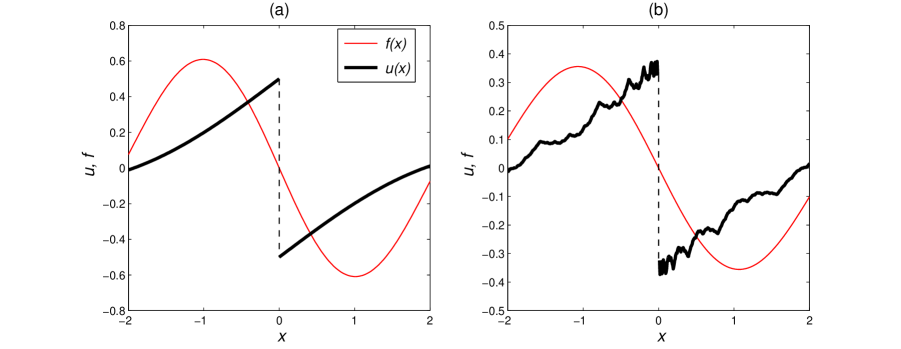
Figure 1: Stationary shock wave solution $u(x)$ (bold line) and forcing $f(x)$ (thin line) for the inviscid continuous model. This solution corresponds to the DN shell model for: (a) forcing $f_{n}=2k_{0}^{1/3}\delta_{n0}$ with the stationary solution (3.21); (b) forcing $f_{n}=2k_{0}^{-1}\delta_{n0}$ with the stationary solution (3.26).

It is instructive to consider a different forcing model, e.g.,

$$f_{n}=2k_{0}^{-1}\delta_{n0}.$$ (3.25)

The fixed-point solution of Eq. (3.19) with the new forcing term (3.25) is

$$u_{n}=k_{0}^{-2/3}k_{n}^{-1/3},\quad n\geq 0.$$ (3.26)

The Fourier transformed forcing $f(k)$ and solution $u(k)$ are given by Eq. (3.22). The corresponding functions $f(x)$ and $u(x)$ in physical space can found analytically or numerically, e.g., using the inverse Fourier transform method described in [2]. These functions are shown in Fig. 1(b). The forcing $f(x)$ is an analytic function, while the solution $u(x)$ has a discontinuity at the origin. For $x\neq 0$, the function $u(x)$ is continuous with the fractal-like shape.

The shell model solution (3.21) has the infinite norm $\sum_{n\in\mathbb{Z}}k_{n}^{2}u_{n}^{2}=\infty$ and it is dissipative [6], i.e., it does not satisfy the energy conservation relation (2.13) even though the model has no viscosity, $\nu=0$. Also, the solution (3.21) was shown (in the case of $\lambda=2^{5/2}$) to be a global attractor for finite energy initial conditions [6]. These two facts get the clear interpretation in physical space: the global attractor is a shock wave, which represents the dissipative mechanism. This mechanism is similar to that known for weak solutions (shocks) of inviscid scalar conservation laws with the flux function $g=g(u)$ in Eq. (2.1), e.g., for the inviscid Burgers equation.

As we mentioned earlier, solutions of the inviscid DN model are unique and conserve the energy (in the absence of forcing), if the norm $\sum_{n\in\mathbb{Z}}k_{n}^{2}u_{n}^{2}<\infty$. This norm becomes infinite (blows up) in finite time [10, 15, 6]. The asymptotic blowup structure is self-similar and universal, and it can be described using the renormalization technique [10, 22]. Following the derivations similar to Eqs. (3.13)–(3.16), one can relate the above norm with the integral $\int|k|^{3}|u(k)|^{2}dk$ for the Fourier transformed continuous solution. This suggests that the physical space solution $u(x,t)$ should be understood in the strong sense before the blowup and in the weak sense after the blowup similarly to the shell models [8]; these questions require further elaboration and are beyond the scope of this paper.

3.3 Viscous solutions

Now let us consider the viscous DN shell model (3.10). We assume the stationary forcing terms (3.25) and choose the viscous coefficients in the form

$$\nu_{n}=\nu k_{0}^{-4/3}k_{n}^{4/3}=\nu\lambda^{4n/3},$$ (3.27)

where $\nu>0$ is a small viscosity parameter. The viscous coefficients (3.27), whose original form was given in Eq. (3.9), are modified in order to facilitate the construction of the continuous solution $u(x,t)$. One can expect that such changes are only important at viscous scales (large $k$), leading to the same behavior in the vanishing viscosity limit $\nu\to+0$ [19].

Substituting Eqs. (3.25) and (3.27) into the DN shell model (3.10) with $k_{n}=k_{0}\lambda^{n}$, yields

$$\frac{\partial U_{n}}{\partial t}=\lambda^{n}U_{n-1}^{2}-\lambda^{n+1}U_{n}U_{n+1}-\nu\lambda^{4n/3}U_{n}+2\delta_{n0},\quad U_{n}=k_{0}u_{n},$$ (3.28)

where we multiplied both sides by $k_{0}$. This representation allows constructing particular solutions $\{u_{n}(k_{0},t)\}_{n\geq 0}$ for any value of the parameter $k_{0}$ using a single solution $\{U_{n}(t)\}_{n\geq 0}$. As the initial condition at $t=0$, we will consider vanishing shell velocities $U_{n}(0)=0$ for all shells $n$.

Due to the viscous coefficients (3.27), which grow as $\lambda^{4n/3}=2^{2n}$, the shell speeds decay rapidly for large $n$. Thus, the numerical solution can be obtained with high accuracy using a finite number of shell velocities $u_{n}$ with $n=0,\ldots,N$ and assuming vanishing velocities for other shells (for example, for $\nu=10^{-4}$, one has $u_{20}\sim 10^{-25}$). The numerical solutions are shown in Fig. 2. One can observe the special behavior near $t_{*}\approx 0.691$ in Fig. 2(a), which corresponds to the viscous coefficient $\nu=0.1$. In the vanishing viscosity limit $\nu\to+0$, the point $t_{*}$ corresponds to a finite time blowup, see Fig. 2(b). For larger times, a steady state is formed.

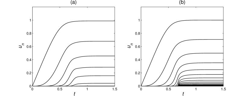
Figure 2: Solutions of the DN shell model with constant forcing (3.25) and zero initial conditions: (a) viscous coefficient $\nu=0.1$, (b) viscous coefficient $\nu=10^{-5}$.

For constructing the corresponding solution of the continuous model, we use Eqs. (3.13) and (3.28), which yield the Fourier transformed solution $u(k,t)$. The inverse Fourier transform (performed numerically as described in [2]) yields the solution $u(x,t)$ in physical space. Figure 3 shows the solution $u(x,t)$ corresponding to the DN model with two different viscous coefficients, $\nu=0.1$ and $\nu=0.01$. These solutions demonstrate the formation of a smooth standing wave. For small viscosity, this solution converges to the inviscid solution described earlier, i.e., to the finite time blowup followed by formation of a shock wave. The blowup point corresponds to $x=u=0$ and $t_{*}\approx 0.691$, as obtained from the shell model solution in Fig. 2(b). This point is shown in Fig. 3(b) by a bold red point. Also, for comparison, this figure shows the stationary solution of the inviscid model (bold blue line located at $t=1.5$), which was obtained earlier in Fig. 1(b).

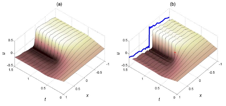
Figure 3: Physical space solutions $u(x,t)$ induced by solutions of the viscous DN shell model with constant forcing (3.25) and zero initial conditions: (a) viscous coefficient $\nu=0.1$, (b) viscous coefficient $\nu=0.01$. The red point in the right figure shows the location of blowup for the inviscid system. Also, the right figure shows the stationary solution of the inviscid model (bold blue line located at $t=1.5$), see Fig. 1(b).

We conclude that physical space solutions $u(x,t)$, which are induced by solutions of the DN shell model, are similar to solutions of scalar conservation laws: a shock wave is formed in finite time in the inviscid model, while the viscosity transforms this shock into a smooth wave solution.

4 Continuous representation of the Sabra model

In this section, we consider the one-dimensional hydrodynamic model (2.1)–(2.3) given by the function

$$\varphi(\xi)=\frac{\psi(\xi)+\psi(1-\xi)}{2},\quad\psi(\xi)=-\sigma^{3}\delta(\xi-\sigma^{2})+(1+c)\delta(\xi-\sigma)+c\sigma^{-3}\delta\left(\xi-\sigma^{-1}\right),$$ (4.1)

where $c$ is a constant real parameter and $\sigma=(1+\sqrt{5})/2\approx 1.618$ is the golden ratio satisfying the equation

$$1+\sigma=\sigma^{2}.$$ (4.2)

After substituting expression (4.1) into Eq. (2.3), the lengthy derivations similar to Eq. (3.3) with the use of Eq. (4.2) yield the kernel of the continuous model in the form

$$K(y,z)=K_{\psi}(y,z)+K_{\psi}(z,y),\quad K_{\psi}(y,z)=\frac{\sigma}{(\sigma y-z)^{2}}-\frac{(1+c)\sigma^{2}}{(\sigma^{2}y-z)^{2}}-\frac{c\sigma}{(\sigma y+z)^{2}}.$$ (4.3)

Singular integrals in Eq. (2.2) must be taken with the Hadamard regularization.

The Fourier transformed continuous model is obtained by substituting function (4.1) into Eq. (2.5). Using relations (3.2) and (4.2), this yields

$$\begin{array}[]{rcl}\displaystyle\frac{\partial u(k)}{\partial t}&=&\displaystyle-ik|k|\left(-\sigma^{3}u(\sigma^{2}k)u(-\sigma k)+(1+c)u(\sigma k)u(-\sigma^{-1}k)+c\sigma^{-3}u(\sigma^{-1}k)u(\sigma^{-2}k)\right)\\[12.0pt] &&\displaystyle-\nu|k|^{2\alpha}u(k)+f(k).\end{array}$$ (4.4)

Now let us define the geometric progression

$$k_{n}=k_{0}\lambda^{n},\quad\lambda=\sigma^{3/2}=\sqrt{2+\sqrt{5}}\approx 2.058,\quad n\in\mathbb{Z},$$ (4.5)

with $1\leq k_{0}<\lambda$, and introduce the corresponding variables

$$u_{n}=k_{n}^{1/3}u\left(k_{n}^{2/3}\right),\quad f_{n}=k_{n}^{1/3}f\left(k_{n}^{2/3}\right).$$ (4.6)

Then Eq. (4.4) taken for $k=k_{n}^{2/3}=k_{0}^{2/3}\sigma^{n}$ reduces to the form

$$\frac{\partial u_{n}}{\partial t}=i\left[k_{n+1}u_{n+2}u^{*}_{n+1}-(1+c)k_{n}u_{n+1}u^{*}_{n-1}-ck_{n-1}u_{n-1}u_{n-2}\right]-\nu_{n}u_{n}+f_{n},\quad n\in\mathbb{Z},$$ (4.7)

where we used the reality condition $u(-k)=u^{*}(k)$ for negative arguments; the viscous coefficients $\nu_{n}=\nu k_{n}^{4\alpha/3}$ are the same as in Eq. (3.9). The system (4.7) is known as the Sabra shell model of turbulence [17]. The most popular choice of the intershell ratio in the Sabra model is $\lambda=2$, which is very close to the value $\lambda\approx 2.058$ defined by the continuous model.

We have shown that the hydrodynamic model given by Eqs. (2.1)–(2.3) and (4.1) splits into infinite-dimensional subsystems (4.7). Each of these subsystems corresponds to a specific value of the parameter $k_{0}$ from the interval (3.11) and represents the Sabra shell model. Note that the conventional choice of the viscous term $\nu_{n}=\nu k_{n}^{2}$ in the Sabra model corresponds to the exponent $\alpha=3/2$, i.e., to the continuous model with hyperviscosity.

4.1 Energy conservation and Hamiltonian form

This section contains technical derivations verifying the conditions (2.7) and (2.14) for the energy conservation and Hamiltonian structure in the continuous model, leading to the analogous properties of the induced Sabra model.

Using Eqs. (4.1), (4.2) and (3.2), one can check that

$$\psi\left(1-\xi\right) = -\sigma^{3}\delta(\xi+\sigma)+(1+c)\delta(\xi+\sigma^{-1})+c\sigma^{-3}\delta(\xi-\sigma^{-2}),$$ (4.8)

$$\psi\left(\frac{1}{\xi}\right) = -\sigma^{-1}\delta(\xi-\sigma^{-2})+(1+c)\sigma^{-2}\delta(\xi-\sigma^{-1})+c\sigma^{-1}\delta(\xi-\sigma),$$ (4.9)

$$\psi\left(1-\frac{1}{\xi}\right) = -\sigma\delta(\xi+\sigma^{-1})+(1+c)\sigma^{2}\delta(\xi+\sigma)+c\sigma\delta(\xi-\sigma^{2}),$$ (4.10)

$$\psi\left(\frac{1}{1-\xi}\right) = -\sigma^{-1}\delta(\xi-\sigma^{-1})+(1+c)\sigma^{-2}\delta(\xi-\sigma^{-2})+c\sigma^{-1}\delta(\xi+\sigma^{-1}),$$ (4.11)

$$\psi\left(\frac{\xi}{\xi-1}\right) = -\sigma\delta(\xi-\sigma)+(1+c)\sigma^{2}\delta(\xi-\sigma^{2})+c\sigma\delta(\xi+\sigma),$$ (4.12)

$$-\xi\psi\left(\frac{1}{\xi}\right) = \sigma^{-3}\delta(\xi-\sigma^{-2})-(1+c)\sigma^{-3}\delta(\xi-\sigma^{-1})-c\delta(\xi-\sigma),$$ (4.13)

$$-\xi\psi\left(1-\frac{1}{\xi}\right) = -\delta(\xi+\sigma^{-1})+(1+c)\sigma^{3}\delta(\xi+\sigma)-c\sigma^{3}\delta(\xi-\sigma^{2}),$$ (4.14)

$$(\xi-1)\psi\left(\frac{1}{1-\xi}\right) = \sigma^{-3}\delta(\xi-\sigma^{-1})-(1+c)\sigma^{-3}\delta(\xi-\sigma^{-2})-c\delta(\xi+\sigma^{-1}),$$ (4.15)

$$(\xi-1)\psi\left(\frac{\xi}{\xi-1}\right) = -\delta(\xi-\sigma)+(1+c)\sigma^{3}\delta(\xi-\sigma^{2})-c\sigma^{3}\delta(\xi+\sigma).$$ (4.16)

Since $\varphi(\xi)=\frac{\psi(\xi)+\psi(1-\xi)}{2}$, the energy conservation condition (2.7) reduces to checking that the sum of expression (4.1) for $\psi(\xi)$ and Eqs. (4.8), (4.13)–(4.16) gives zero. It is straightforward to check that this condition holds indeed. The same expressions (3.15) and (3.16) hold for the energy of the continuous system $E$ and for the energy of the Sabra model $E_{s}$.

Energy conservation was one of the criteria for the construction of the Sabra shell model [17]. The unforced inviscid Sabra model (4.7) possesses another quadratic invariant

$$H_{s}=\sum_{n\in\mathbb{Z}}c^{-n}|u_{n}|^{2}.$$ (4.17)

This invariant is associated with the helicity for $c<0$ (not sign-definite invariant) and with the enstrophy for $c>0$ (sign definite invariant); these definitions are physically relevant for $0<|c|<1$.

The Hamiltonian structure condition (2.14) with the function (4.1) takes the form

$$\psi\left(\frac{1}{\xi}\right)+\psi\left(1-\frac{1}{\xi}\right)+\psi\left(\frac{1}{1-\xi}\right)+\psi\left(\frac{\xi}{\xi-1}\right)=2\psi\left(\xi\right)+2\psi\left(1-\xi\right).$$ (4.18)

Using Eqs. (4.1) and (4.8)–(4.12), it is straightforward to check that the condition (4.18) is satisfied if and only if $c=-\sigma^{2}\approx-2.618$. Indeed, using Eqs. (4.2) and (4.5), one can check that the Sabra model (4.7) with $\nu_{n}=f_{n}=0$ and $c=-\sigma^{2}$ can be written in the canonical Hamiltonian form

$$\frac{\partial a_{n}}{\partial t}=-i\frac{\partial H}{\partial a_{n}^{*}}=ik_{n}^{4/3}\left(\sigma^{2}a_{n+2}a_{n+1}^{*}+a_{n+1}a_{n-1}^{*}+\sigma^{-2}a_{n-1}a_{n-2}\right),$$ (4.19)

where $a_{n}=\sigma k_{n}^{-1/3}u_{n}$, and $\{a_{n},a_{n}^{*}\}$ are pairs of complex canonical variables with the Hamiltonian

$$H=-\sum_{n}k_{n}^{4/3}\left(a_{n-1}^{*}a_{n}^{*}a_{n+1}+a_{n-1}a_{n}a_{n+1}^{*}\right).$$ (4.20)

Note that a different Hamiltonian representation of the Sabra model was found in [18] for $c=-\sigma^{-2}\approx-0.382$. It has the form

$$\frac{\partial a_{n}}{\partial t}=-i\frac{\partial H}{\partial a_{n}^{*}},\quad a_{n}=\left\{\begin{array}[]{ll}\sigma^{-1}k_{n}^{1/3}u_{n},&\textrm{even }n;\\[3.0pt] -\sigma^{-1}k_{n}^{1/3}u_{n}^{*},&\textrm{odd }n;\end{array}\right.$$ (4.21)

with the Hamiltonian

$$H=\sum_{n}k_{n}^{2/3}\left(a_{n-1}a_{n}^{*}a_{n+1}^{*}+a_{n-1}^{*}a_{n}a_{n+1}\right).$$ (4.22)

4.2 Inviscid model

Let us consider the unforced inviscid Sabra model

$$\frac{\partial u_{n}}{\partial t}=i\left[k_{n+1}u_{n+2}u^{*}_{n+1}-(1+c)k_{n}u_{n+1}u^{*}_{n-1}-ck_{n-1}u_{n-1}u_{n-2}\right],\quad n\geq 0.$$ (4.23)

Here we assume that all shell speeds $u_{n}$ with $n<0$ vanish. This can be arranged, for example, by considering vanishing initial conditions for shells with $n<0$ and specifying the forcing terms $f_{-2}$ and $f_{-1}$ such that the right-hand sides of the equations for $u_{-2}$ and $u_{-1}$ vanish.

First let us consider the case $c=\lambda^{-2}\approx 0.236$, when the conserved quantity (4.17) is positive and can be associated with the enstrophy. For this reason, Eq. (4.23) with $c=\lambda^{-2}$ is considered to be the shell model for two-dimensional inviscid flow (2D Euler equations). This model has a unique global in time solution for initial conditions of finite energy and enstrophy [8].

Let us consider the complex initial conditions of the form

$$t=0:\quad u_{0}=ik_{0}^{-1},\quad u_{1}=2k_{0}^{-1},\quad u_{n}=0,\quad n\geq 2.$$ (4.24)

Since $k_{n}=k_{0}\lambda^{n}$, the solution of Eq. (4.23) can be written as

$$u_{n}(k_{0},t)=k_{0}^{-1}U_{n}(t),$$ (4.25)

where $U_{n}$ satisfies the equation

$$\frac{\partial U_{n}}{\partial t}=i\left[\lambda^{n+1}U_{n+2}U^{*}_{n+1}-(1+c)\lambda^{n}U_{n+1}U^{*}_{n-1}-c\lambda^{n-1}U_{n-1}U_{n-2}\right],\quad n\geq 0,$$ (4.26)

with the initial conditions

$$t=0:\quad U_{0}=i,\quad U_{1}=2,\quad U_{n}=0,\quad n\geq 2.$$ (4.27)

According to Eqs. (4.5), (4.6) and (4.25), the Fourier transformed solution $u(k,t)$ of the continuous model is given by

$$u(k,t)=k^{-1/2}u_{n}(k_{0},t)=k^{-1/2}k_{0}^{-1}U_{n}(t),\quad k=k_{n}^{2/3}=k_{0}^{2/3}\sigma^{n},$$ (4.28)

with the reality condition $u(-k)=u^{*}(k)$ for negative $k$. Recall that $u(k)=0$ for $k=0$ due to the vanishing mean value condition, $\int u\,dx=0$, assumed in Section 2. The corresponding solution $u(x,t)$ in physical space is given by the inverse Fourier transform.

The solutions can be found numerically with high accuracy by considering a finite number of shells, as it was done in Section 3.3. The numerical results are presented in Fig. 4, showing the physical space representation of the single solution $U_{n}(t)$ for the Sabra model in 2D regime. This solution is smooth as expected due to regularity of the inviscid 2D Sabra model.

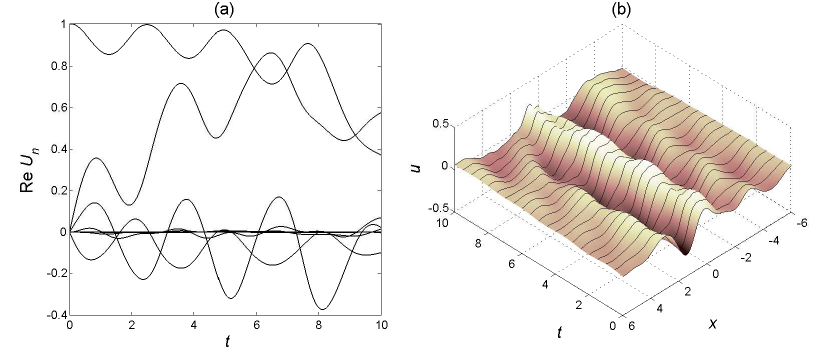
Figure 4: Inviscid Sabra model with no forcing in the 2D regime ($c=\lambda^{-2}$). (a) Evolution of complex shell velocities $U_{n}(t)$ for initial conditions (4.27). Only real parts are shown. (b) Physical space representation $u(x,t)$ of the shell model solution $U_{n}(t)$.

Now let us consider the case $c=-\lambda^{-1}\approx-0.486$. In this case the conserved quantity (4.17) is not sign definite and can be associated with the helicity. For this reason, Eq. (4.23) with $c=-\lambda^{-1}$ is considered as the shell model for three-dimensional inviscid flow (3D Euler equations). For this Sabra model, there exists a unique local in time solution if the initial conditions have the finite norm $\sum_{n}k_{n}^{2}|u_{n}|^{2}<\infty$, see [8]. In general, the solution leads to a finite-time blowup [21] characterized by the infinite norm $\sum_{n}k_{n}^{2}|u_{n}|^{2}\to\infty$ as $t\to t_{b}-0$. This blowup has the self-similar asymptotic form for large shells $n$ and $t\to t_{b}$. This form, up to system symmetries, is given by the expression $u_{n}(t)\to-ik_{n}^{-y}U(k_{n}^{1-y}(t-t_{b}))$, where $y$ and $U(t)$ are the universal real scaling exponent and real function depending only on the Sabra model parameter $c$ [23].

For numerical solution, we consider complex initial conditions (4.24) leading to the solution (4.25) of the system (4.26), (4.27) with $c=-\lambda^{-1}$. The solution $U_{n}(t)$ found numerically is presented in Fig. 5(a). The blowup occurs at $t_{b}\approx 0.716$, and one can recognize the asymptotic self-similar form of this solution developing for large $n$ near the blowup time. The corresponding physical space solution $u(x,t)$ of the continuous model is obtained using Eq. (4.28) with the inverse Fourier transform. The result is shown in Fig. 5(b). One can observe the strongly nonlocal character of the blowup; this is not surprising due to nonlocality of the continuous model (2.1), (2.2).

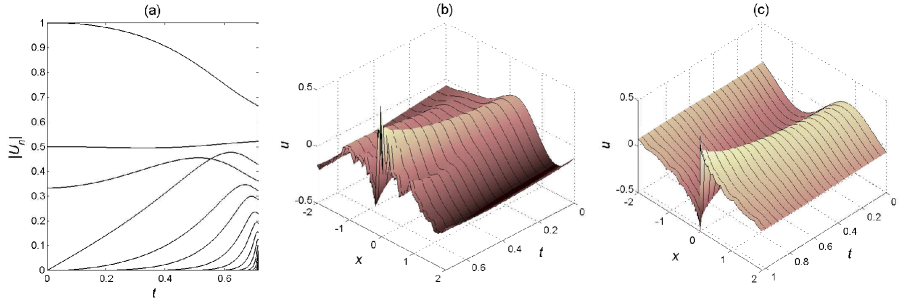
Figure 5: Finite-time blowup in inviscid Sabra model with no forcing in the 3D regime ($c=-\lambda^{-1}$). (a) Evolution of shell speed amplitudes $|U_{n}(t)|$ for complex initial conditions (4.27). (b) Physical space representation $u(x,t)$ of the shell model solution $U_{n}(t)$. (c) Physical space representation $u(x,t)$ of the purely imaginary solution $U_{n}(t)$. The last time in all the figures corresponds to the blowup point.

Despite the similarity of blowup structures for different shell models described by the renormalization method [10, 21, 22], the physical space representation of the blowup turns out to be very different; compare Fig. 5 with the blowup formation described in Figs. 2 and 3. For further insight, Fig. 5(c) shows the blowup with purely imaginary initial conditions ($U_{0}(0)=-i/2$, $U_{1}(0)=-i$, $U_{n}(0)=0$ for $n\geq 2$), which describe odd solutions $u(-x,t)=-u(x,t)$ of the continuous model. In this case, the blowup creates a discontinuity at $x=0$ exactly at the blowup time. Note the difference from Fig. 3 (and also from the Burgers equation), where the discontinuity appears only after the blowup.

4.3 Viscous solutions

In this section, we consider the viscous Sabra model (4.7) with the shells $n\geq 0$ ($u_{n}=0$ for $n<0$). We assume vanishing initial conditions, the constant forcing with two nonzero elements $f_{0}=ik_{0}^{-1}$ and $f_{1}=(1+i)k_{0}^{-1}$, and viscous coefficients $\nu_{n}=\nu\lambda^{2n}=\nu(k_{n}/k_{0})^{2}$. As we already mentioned, such choice of viscous terms corresponds to the continuous model with hyperviscosity.

The shell model solution $u_{n}(k_{0},t)$ can be written in the form (4.25), where $U_{n}$ satisfy the equations

$$\frac{\partial U_{n}}{\partial t}=i\left[\lambda^{n+1}U_{n+2}U^{*}_{n+1}-(1+c)\lambda^{n}U_{n+1}U^{*}_{n-1}-c\lambda^{n-1}U_{n-1}U_{n-2}\right]+\nu\lambda^{2n}U_{n}+F_{n}$$ (4.29)

for $n\geq 0$ with the nonzero forcing terms $F_{0}=i$, $F_{1}=1+i$ and vanishing initial conditions. Thus, a single solution $U_{n}(t)$ can be used to reconstruct the dynamics for all $k_{0}$. Then, the continuous model solution $u(k,t)$ is obtained using Eq. (4.28) for positive $k$ and using the reality condition $u(-k)=u^{*}(k)$ for negative $k$. The corresponding solution $u(x,t)$ in physical space is given by the inverse Fourier transform.

Figure 6(a) presents the results of numerical simulations for the Sabra model (4.29). The singularity occurs near $t\approx 1.27$. This singularity corresponds to blowup in the inviscid system, while it is depleted at large shell numbers in the viscous model. After the transient period around $1.27<t<2.48$, the system enters into the intermittent turbulent regime. It is known that, in this regime, the inertial interval of scales (shells) is created, where the velocity moments scale as power-laws with the anomalous scaling exponents close to those in the Navier-Stokes turbulence [17, 11]. The intermittent regime is characterized by a sequence of turbulent bursts. These bursts (also called instantons) have self-similar statistics for the Sabra model [20], directly related to the anomalous scaling [23].

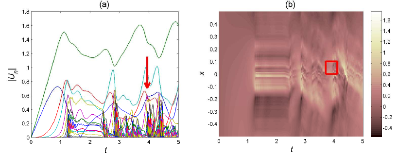
Figure 6: (a) Dynamics of velocity amplitudes $|U_{n}(t)|$ for the Sabra model in 3D regime ($c=-\lambda^{-1}$) for constant forcing and viscous coefficient $\nu=10^{-5}$. (b) Physical space representation $u(x,t)$ of the shell model solution. The red box in the right figure shows the part amplified in Fig. 7; it corresponds to the formation of a turbulent burst pointed by the arrow in the left figure.

Figure 6(b) presents the corresponding solution of the continuous model (2.1) in the physical space $(x,t)$. One can see that the turbulent behavior is localized in the region around the origin, $x=0$, due to localization of the constant forcing term $f(x)$. A sequence of turbulent bursts in physical space can be recognized, which correspond to the instantons in the Sabra shell model solution in Fig. 6(a). We have chosen a specific instanton near $t\approx 4$ and showed its detailed structure for both shell amplitudes $|U_{n}|$ and physical space function $u(x,t)$ in Fig. 7.

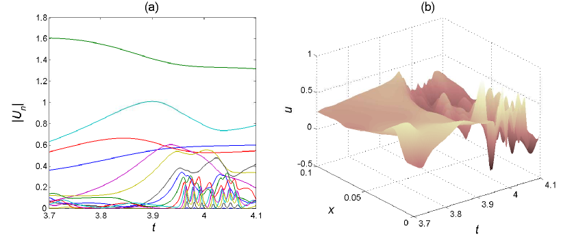
Figure 7: Dynamics of velocity amplitudes $|U_{n}(t)|$ for the Sabra model in 3D regime ($c=-\lambda^{-1}$) and the corresponding physical space representation $u(x,t)$. The presented plots correspond to the specific turbulent burst indicated in Fig. 6.

5 Conclusion

In this paper we constructed continuous hydrodynamic models, which reduce after the Fourier transformation to an infinite set of equivalent shell models. These continuous models share various properties of the Navier-Stokes equations like the scaling invariance, nonlocal quadratic term, energy conservation (for the inviscid system), etc. We also discuss their Hamiltonian representations. Such constructions are carried out for the dyadic (Desnyansky–Novikov) model with the intershell ratio $\lambda=2^{3/2}$ and for the Sabra model of turbulence with $\lambda=\sqrt{2+\sqrt{5}}\approx 2.058$. Note that the values of $\lambda$ allowing the continuous representation are fixed and no limit like $\lambda\to 1$ is necessary.

The constructed continuous models allow understanding various properties of the discrete shell models and provide their interpretation in physical space. This is especially pronounced for the dyadic shell model, where the asymptotic solution with Kolmogorov scaling, $u_{n}\propto k_{n}^{-1/3}$, is represented by a shock (discontinuity) for the induced continuous solution in physical space. Moreover, the finite-time blowup together with its viscous regularization in the continuous model follow the scenario similar to the Burgers equation. For the Sabra model, we provide the physical space representation for both blowup solution and intermittent turbulent dynamics. There is a drastic difference of these phenomena in physical space in comparison with the dyadic model.

As a future research topic, it would be interesting to study the relation between the turbulent statistics of the Sabra model solutions with physical space properties of the corresponding intermittent continuous solutions. It is reasonable to expect the formation of inertial interval in the continuous model with the anomalous scaling for velocity moments [11] driven by similar dynamics of the Sabra model [17, 3]. This relation is not expected to be simple. For example, the asymptotic solution of the dyadic shell model has the Kolmogorov scaling, while the shocks in the continuous representation should lead to the anomalous scaling similar to the Burgers equation turbulence [4].

References

- [1] K.H. Andersen, T. Bohr, M.H. Jensen, J.L. Nielsen, and P. Olesen. Pulses in the zero-spacing limit of the GOY model. Physica D, 138:44–62, 2000.
- [2] D.H. Bailey and P.N. Swarztrauber. A fast method for the numerical evaluation of continuous Fourier and Laplace transforms. SIAM Journal on Scientific Computing, 15(5):1105–1110, 1994.
- [3] L. Biferale. Shell models of energy cascade in turbulence. Annu. Rev. Fluid Mech., 35(1):441–468, 2003.
- [4] J. Cardy, G. Falkovich, and K. Gawedzki. Non-equilibrium Statistical Mechanics and Turbulence. Cambridge University Press, 2008.
- [5] A. Cheskidov. Blow-up in finite time for the dyadic model of the Navier–Stokes equations. Transactions of the American Mathematical Society, 360(10):5101–5120, 2008.
- [6] A. Cheskidov, S. Friedlander, and N. Pavlović. Inviscid dyadic model of turbulence: the fixed point and Onsager’s conjecture. Journal of Mathematical Physics, 48(6):065503, 2007.
- [7] A. Cheskidov, S. Friedlander, and N. Pavlović. An inviscid dyadic model of turbulence: The global attractor. Discrete and Continuous Dynamical Systems, 26(3):781–794, 2010.
- [8] P. Constantin, B. Levant, and E. S. Titi. Regularity of inviscid shell models of turbulence. Phys. Rev. E, 75(1):016304, 2007.
- [9] V.N. Desnyansky and E.A. Novikov. The evolution of turbulence spectra to the similarity regime. Izv. A.N. SSSR Fiz. Atmos. Okeana, 10(2):127–136, 1974.
- [10] T. Dombre and J.L. Gilson. Intermittency, chaos and singular fluctuations in the mixed Obukhov–Novikov shell model of turbulence. Physica D, 111(1–4):265–287, 1998.
- [11] U. Frisch. Turbulence: The Legacy of A.N. Kolmogorov. Cambridge University Press, 1995.
- [12] C.S. Gardner. Korteweg–de Vries equation and generalizations. IV. The Korteweg–de Vries equation as a Hamiltonian system. J. Math. Phys., 12(8):1548–1551, 1971.
- [13] E.B. Gledzer. System of hydrodynamic type admitting two quadratic integrals of motion. Sov. Phys. Doklady, 18:216, 1973.
- [14] R.P. Kanwal. Generalized functions: theory and applications. Springer, 2004.
- [15] N.H. Katz and N. Pavlovic. Finite time blow-up for a dyadic model of the Euler equations. Transactions of the American Mathematical Society, 357(2):695–708, 2005.
- [16] E.N. Lorenz. Low order models representing realizations of turbulence. Journal of Fluid Mechanics, 55:545–563, 1972.
- [17] V.S. L’vov, E. Podivilov, A. Pomyalov, I. Procaccia, and D. Vandembroucq. Improved shell model of turbulence. Phys. Rev. E, 58(2):1811, 1998.
- [18] V.S. L’vov, E. Podivilov, and I. Procaccia. Hamiltonian structure of the Sabra shell model of turbulence: exact calculation of an anomalous scaling exponent. EPL (Europhysics Letters), 46:609–612, 1999.
- [19] V.S. L’vov, I. Procaccia, and D. Vandembroucq. Universal scaling exponents in shell models of turbulence: viscous effects are finite-sized corrections to scaling. Phys. Rev. Lett., 81:802–805, 1998.
- [20] A.A. Mailybaev. Computation of anomalous scaling exponents of turbulence from self-similar instanton dynamics. Phys. Rev. E, 86(2):025301, 2012.
- [21] A.A. Mailybaev. Renormalization and universality of blowup in hydrodynamic flows. Phys. Rev. E, 85(6):066317, 2012.
- [22] A.A. Mailybaev. Bifurcations of blowup in inviscid shell models of convective turbulence. Nonlinearity, 26:1105–1124, 2013.
- [23] A.A. Mailybaev. Blowup as a driving mechanism of turbulence in shell models. Physical Review E, 87(5):053011, 2013.
- [24] P.J. Morrison. Hamiltonian description of the ideal fluid. Rev. Mod. Phys., 70:467–521, 1998.
- [25] K. Ohkitani and M. Yamada. Temporal intermittency in the energy cascade process and local Lyapunov analysis in fully developed model of turbulence. Prog. Theor. Phys., 89:329–341, 1989.
- [26] F. Waleffe. On some dyadic models of the Euler equations. Proceedings of the American Mathematical Society, 134(10):2913–2922, 2006.