Non-linear Causal Inference using Gaussianity Measures

Abstract

We provide theoretical and empirical evidence for a type of asymmetry between causes and effects that is present when these are related via linear models contaminated with additive non-Gaussian noise. Assuming that the causes and the effects have the same distribution, we show that the distribution of the residuals of a linear fit in the anti-causal direction is closer to a Gaussian than the distribution of the residuals in the causal direction. This Gaussianization effect is characterized by reduction of the magnitude of the high-order cumulants and by an increment of the differential entropy of the residuals. The problem of non-linear causal inference is addressed by performing an embedding in an expanded feature space, in which the relation between causes and effects can be assumed to be linear. The effectiveness of a method to discriminate between causes and effects based on this type of asymmetry is illustrated in a variety of experiments using different measures of Gaussianity. The proposed method is shown to be competitive with state-of-the-art techniques for causal inference.

Keywords: causal inference, Gaussianity of the residuals, cause-effect pairs

1 Introduction

The inference of causal relationships from data is one of the current areas of interest in the artificial intelligence community, e.g. (Chen et al., 2014; Janzing et al., 2012; Morales-Mombiela et al., 2013). The reason for this surge of interest is that discovering the causal structure of a complex system provides an explicit description of the mechanisms that generate the data, and allows us to understand the consequences of interventions in the system (Pearl, 2000). More precisely, automatic causal inference can be used to determine how modifications of the value of certain relevant variables (the causes) influence the values of other related variables (the effects). Therefore, understanding cause-effect relations is of paramount importance to control the behavior of complex systems and has applications in industrial processes, medicine, genetics, economics, social sciences or meteorology.

Causal relations can be determined in complex systems in three different ways. First, they can be inferred from domain knowledge provided by an expert, and incorporated in an ad-hoc manner in the description of the system. Second, they can be discovered by performing interventions in the system. These are controlled experiments in which one or several variables of the system are forced to take particular values. Interventions constitute a primary tool for identifying causal relationships. However, in many situations they are unethical, expensive, or technically infeasible. Third, they can be estimated using causal discovery algorithms that use as input purely uncontrolled and static data.

This last approach for causal discovery has recently received much attention from the machine learning community (Shimizu et al., 2006; Hoyer et al., 2009; Zhang and Hyvärinen, 2009). These methods assume a particular model for the mapping mechanisms that link causes to effects. By specifying particular conditions on the mapping mechanism and the distributions of the cause and noise variables, the causal direction becomes identifiable Chen et al. (2014). For instance, Hoyer et al. (2009) assume that the effect is a non-linear transformation of the cause plus some independent additive noise. A potential drawback of these methods is that the assumptions made by the particular model considered could be unrealistic for the data under study.

In this paper we propose a general method for causal inference that belongs to the third of the categories described above. Specifically, we assume that the cause and the effect variables have the same distribution and are linked by a linear relationship contaminated with non-Gaussian noise. For the univariate case we prove that, under these assumptions, the magnitude of the cumulants of the residuals of order higher than two is smaller for the linear fit in the anti-causal direction than in the causal one. Since the Gaussian is the only distribution whose cumulants of order higher than 2 are zero, statistical tests based on measures of Gaussianity can be used for causal inference. An antecedent of this result is the observation that, when cause and effect have the same distribution, the residuals of a fit in the anti-causal direction have higher entropy than in the causal direction (Hyvärinen and Smith, 2013; Kpotufe et al., 2014). Since the residuals of the causal and anti-causal linear models have the same variance and the Gaussian is the distribution that maximizes the entropy for a fixed variance, this means that the distribution of the latter is more Gaussian than the former.

For multivariate cause-effect pairs that have the same distribution and are related by a linear model with additive non-Gaussian noise the proof given by (Hyvärinen and Smith, 2013; Kpotufe et al., 2014) can be extended to show that the entropy of the vector of residuals of a linear fit in the anti-causal direction is larger than the corresponding residuals of a linear fit in the causal direction. We conjecture that also in this case there is a reduction of the magnitude of the tensor cumulants of the anti-causal multivariate residuals and provide some numerical evidence of this effect in two dimensions.

The problem of non-linear causal inference is addressed by embedding the original problem in an expanded feature space. We then make the assumption that the non-linear relation between causes and effects in the original space is linear in the expanded feature space. The computations required to make inference on the causal direction based on this embedding can be readily carried out using kernel methods.

In summary, the proposed method for causal inference proceeds by first making a transformation of the original variables so that causes and effects have the same distribution. Then we perform kernel ridge regression in both the causal and the anti-causal directions. The dependence between causes and effects, which is non-linear in the original space, is assumed to be linear in the kernel-induced feature space. A statistical test is then used to quantify the degree of similarity between the distributions of these residuals and a Gaussian distribution with the same variance. Finally, the direction in which the residuals are less Gaussian is identified as the causal one.

The performance of this method is evaluated in both synthetic and real-world cause-effect pairs. From the results obtained it is apparent that the anti-causal residuals of a linear fit in the expanded feature space are more Gaussian than the causal residuals. In general, it is difficult to estimate the entropy from a finite sample (Beirlant et al., 1997). Empirical estimators of high order cumulants involve high order moments, which means they often have large variance. As an alternative, we propose to use statistical tests based on the energy distance to characterize the Gaussianization effect for the residuals of linear fits in the causal and anti-causal directions. Tests based on the energy distance were analyzed in depth in (Székely and Rizzo, 2005). They have been shown to be related to homogeneity tests based on embeddings in a Reproducing Kernel Hilbert Space in (Gretton et al., 2012). An advantage of energy distance-based statistics is that they can be readily estimated from a sample by computing expectations of pairwise Euclidean distances. The energy distance generally provides better results than the entropy or cumulant-based Gaussianity measures. In the problems investigated, the accuracy of the proposed method, using the energy distance to the Gaussian, is comparable to other state-of-the-art techniques for causal discovery.

The rest of the paper is organized as follows: Section 2 illustrates that, under certain conditions, the residuals of a linear regression fit are closer to a Gaussian in the anti-causal direction than in the causal one, based on a reduction of the high-order cumulants and on an increment of the entropy. This section considers both the univariate and multivariate cases. Section 3 adopts a kernel approach to carry out a feature expansion that can be used to detect non-linear causal relationships. We also show here how to compute the residuals in the expanded feature space, and how to choose the different hyper-parameters of the proposed method. Section 4 contains a detailed description of the implementation. In section 6 we present the results of an empirical assessment of the proposed method in both synthetic and real-world cause-effect data pairs. Finally, Section 7 summarizes the conclusions and puts forth some ideas for future research.

2 Asymmetry based on the non-Gaussianity of the residuals of linear models

Let $\mathcal{X}$ and $\mathcal{Y}$ be two random variables that are causally related. The direction of the causal relation is not known. Our goal is to determine whether $\mathcal{X}$ causes $\mathcal{Y}$, i.e., $\mathcal{X}\rightarrow\mathcal{Y}$ or, alternatively $\mathcal{Y}$ causes $\mathcal{X}$, i.e., $\mathcal{Y}\rightarrow\mathcal{X}$. For this purpose, we exploit an asymmetry between causes an effects. This type of asymmetry can be uncovered using statistical tests that measure the non-Gaussianity of the residuals of linear regression models obtained from fits in the causal and in the anti-causal direction.

To motivate the methodology that we have developed, we will proceed in stepwise manner. First we analyze a special case in one dimension: We assume that $\mathcal{X}$ and $\mathcal{Y}$ have the same distribution and are related via a linear model contaminated with additive i.i.d. non-Gaussian noise. The noise is independent of the cause. Under these assumptions we show that the distribution of the residuals of a linear fit in the incorrect (anti-causal) direction is closer to a Gaussian distribution than the distribution of the residuals in the correct (causal) direction. For this, we use an argument based on the reduction of the magnitude of the cumulants of order higher than 2. The cumulants are defined as the derivatives of the logarithm of the moment-generating function evaluated at zero (Cornish and Fisher, 1938; McCullagh, 1987).

The Gaussianization effect can be characterized also in terms of an increase of the entropy. The proof is based on the results of (Hyvärinen and Smith, 2013), which are extended in this paper to the multivariate case. In particular, we show that the entropy of the residuals of a linear fit in the anti-causal direction is larger or equal than the entropy of the residuals of a linear fit in the causal direction. Since the Gaussian it the distribution that has maximum entropy, given a particular covariance matrix, an increase of the entropy of the residuals means that their distribution becomes closer to the Gaussian.

Finally, we note that it is easy to guarantee that $\mathcal{X}$ and $\mathcal{Y}$ have the same distribution in the case that these variables are unidimensional and continuous. To this end we only have to transform one of the variables (typically the cause random variable) using the probability integral transform, as described in Section 4. However, after the data have been transformed, the relation between the variables will no longer be linear in general. Thus, to address non-linear cause-effect problems involving univariate random variables the linear model is formulated in an expanded feature space, where the multivariate analysis of the Gaussianization effect is also applicable. In this feature space all the computations required for causal inference can be formulated in terms of kernels. This can be used to detect non-linear causal relations in the original input space and allows for an efficient implementation of the method. The only assumption is that the non-linear relation in the original input space is linear in the expanded feature space induced by the selected kernel.

2.1 Analysis of the univariate case based on cumulants

Let $\mathcal{X}$ and $\mathcal{Y}$ be one-dimensional random variables that have the same distribution. Without further loss of generality, we will assume that they have zero mean and unit variance. Let $\mathbf{x}=(x_{1},\ldots,x_{N})^{\text{T}}$ and $\mathbf{y}=(y_{1},\ldots,y_{N})^{\text{T}}$ be $N$ paired samples drawn i.i.d. from $P(\mathcal{X},\mathcal{Y})$. Assume that the causal direction is $\mathcal{X}\rightarrow\mathcal{Y}$ and that the measurements are related by a linear model

$$y_{i} =wx_{i}+\epsilon_{i}\,,\quad\epsilon_{i}\,\bot\,x_{i}\,,\quad\forall i\,,$$ (1)

where $w=\text{corr}(\mathcal{X},\mathcal{Y})\in[-1,1]$ and $\epsilon_{i}$ is independent i.d. non-Gaussian additive noise.

A linear model in the opposite direction, i.e., $\mathcal{Y}\rightarrow\mathcal{X}$, can be built using least squares

$$x_{i}=wy_{i}+\tilde{\epsilon}_{i},$$ (2)

where $w=\text{corr}(\mathcal{Y},\mathcal{X})$ is the same coefficient as in the previous model. The residuals of this reversed linear model are defined as $\tilde{\epsilon}_{i}=x_{i}-wy_{i}$.

Following an argument similar to that of Hernández-Lobato et al. (2011) we show that the residuals $\{\tilde{\epsilon}_{i}\}_{i=1}^{N}$ in the anti-causal direction are more Gaussian than the residuals $\{\epsilon_{i}\}_{i=1}^{N}$ in the actual causal direction $\mathcal{X}\rightarrow\mathcal{Y}$ based on a reduction of the magnitude of the cumulants. The proof is based on establishing a relation between the cumulants of the distribution of the residuals in both the causal and the anti-causal direction. First, we show that $\kappa_{n}(y_{i})$, the $n$-th order cumulant of $\mathcal{Y}$, can be expressed in terms of $\kappa_{n}(\epsilon_{i})$, the $n$-th order cumulant of the residuals:

$$\kappa_{n}(y_{i}) =w^{n}\kappa_{n}(x_{i})+\kappa_{n}(\epsilon_{i})=w^{n}\kappa_{n}(y_{i})+\kappa_{n}(\epsilon_{i})=\frac{1}{1-w^{n}}\kappa_{n}(\epsilon_{i})\,.$$ (3)

To derive this relation we have used (1), that $x_{i}$ and $y_{i}$ have the same distribution (and hence have the same cumulants), and standard properties of cumulants (Cornish and Fisher, 1938; McCullagh, 1987). Furthermore,

$$\kappa_{n}(\tilde{\epsilon}_{i}) =\kappa_{n}(x_{i}-wy_{i})=\kappa_{n}(x_{i}-w^{2}x_{i}-w\epsilon_{i})=(1-w^{2})^{n}\kappa_{n}(x_{i})+(-w)^{n}\kappa_{n}(\epsilon_{i})$$

$$=(1-w^{2})^{n}\kappa_{n}(y_{i})+(-w)^{n}\kappa_{n}(\epsilon_{i})=\frac{(1-w^{2})^{n}}{1-w^{n}}\kappa_{n}(\epsilon_{i})+(-w)^{n}\kappa_{n}(\epsilon_{i})$$

$$=c_{n}(w)\kappa_{n}(\epsilon_{i})\,,$$ (4)

where we have used the definition of $\tilde{\epsilon_{i}}$ and (3) In Figure 1 the value of

$$c_{n}(w)=\frac{(1-w^{2})^{n}}{1-w^{n}}+(-w)^{n}.$$ (5)

is displayed as a function of $w\in[-1,1]$. Note that $c_{1}(w)=c_{2}(w)=1$ independently of the value of $w$. This means that the mean and the variance of the residuals are the same in both the causal and anti-causal directions. For $n>2$, $|c_{n}(w)|\leq 1$ with equality only for $w=0$ and $w=\pm 1$. The result is that the high-order cumulants of the residuals in the anti-causal direction are smaller in magnitude that the corresponding cumulants in the causal direction. Using the observation that all the cumulants of the Gaussian distribution of order higher than two are zero (Marcinkiewicz, 1938), we conclude that the distribution of the residuals in the anti-causal direction is closer to the Gaussian distribution than in the causal direction.

Figure 1: Values of the function $c_{n}(\cdot)$ as a function of $w$ for each cumulant number $n$ (odd in the left plot, even in the right plot). All values for $c_{n}(\cdot)$ lie in the interval $[-1,1]$.

In summary, we can infer the causal direction by (i) fitting a linear model in each possible direction, i.e., $\mathcal{X}\rightarrow\mathcal{Y}$ and $\mathcal{Y}\rightarrow\mathcal{X}$, and (ii) carrying out statistical tests to detect the level of Gaussianity of the two corresponding residuals. The direction in which the residuals are less Gaussian is expected to be the correct one.

2.2 Analysis of the multivariate case based on cumulants

In this section we argue that the Gaussianization effect of the residuals in the anti-causal direction also takes place when the two random variables $\mathcal{X}$ and $\mathcal{Y}$ are multidimensional. We will assume that these variables follow the same distribution and, without further loss of generality, that they have been whitened (i.e., they have a zero mean vector and the identity matrix as the covariance matrix). Let $\mathbf{X}=(\mathbf{x}_{1},\ldots,\mathbf{x}_{N})^{\text{T}}$ and $\mathbf{Y}=(\mathbf{y}_{1},\ldots,\mathbf{y}_{N})^{\text{T}}$ be $N$ paired samples drawn i.i.d. from $P(\mathcal{X},\mathcal{Y})$. In this case, the model assumed for the actual causal relation is

$$\mathbf{y}_{i}=\mathbf{A}\mathbf{x}_{i}+\bm{\epsilon}_{i}\,,\quad\bm{\epsilon}_{i}\,\bot\,\mathbf{x}_{i}\,,\quad\forall i\,,$$ (6)

where $\mathbf{A}=\text{corr}(\mathcal{Y},\mathcal{X})$ is a $d\times d$ matrix of model coefficients and $\bm{\epsilon}_{i}$ is i.i.d. non-Gaussian additive noise. The model in the anti-causal direction is the one that results from the least squares fit:

$$\mathbf{x}_{i} =\tilde{\mathbf{A}}\mathbf{y}_{i}+\tilde{\bm{\epsilon}}_{i}\,,$$ (7)

where we have defined $\tilde{\bm{\epsilon}}_{i}=\mathbf{x}_{i}-\tilde{\mathbf{A}}\mathbf{y}_{i}$ and $\tilde{\mathbf{A}}=\text{corr}(\mathcal{X},\mathcal{Y})=\mathbf{A}^{\text{T}}$.

As in the univariate case, we start by expressing the cumulants of $\mathcal{Y}$ in terms of the cumulants of the residuals. However, the cumulants are now tensors (McCullagh, 1987):

$$\kappa_{n}(\mathbf{y}_{i}) =\kappa_{n}(\mathbf{A}\mathbf{x}_{i})+\kappa_{n}(\bm{\epsilon}_{i})\,.$$ (8)

In what follows, the notation $\text{vect}(\cdot)$ stands for the vectorization of a tensor. For example, in the case of a tensor $\mathbf{T}$ with dimensions $d\times d\times d$

$$\text{vect}(\mathbf{T})=(T_{1,1,1},T_{2,1,1},\cdots,T_{d,1,1},T_{1,2,1},\cdots,T_{d,d,d})^{\text{T}}.$$

Using this notation we obtain

$$\text{vect}(\kappa_{n}(\mathbf{y}_{i})) =\mathbf{A}^{n}\text{vect}(\kappa_{n}(\mathbf{x}_{i}))+\text{vect}(\kappa_{n}(\bm{\epsilon}))=(\mathbf{I}-\mathbf{A}^{n})^{-1}\text{vect}(\kappa_{n}(\bm{\epsilon}))\,,$$ (9)

where $\mathbf{A}^{n}=\mathbf{A}\otimes\mathbf{A}\otimes\mathbf{A}\cdots\otimes\mathbf{A}$, $n$ times, is computed using the Kronecker matrix product. To derive this expression we have used (6), the fact that $\mathcal{Y}$ and $\mathcal{X}$ are equally distributed and hence have the same cumulants. We also have used the properties of the tensor cumulants $\text{vect}(\kappa_{n}(\mathbf{A}\mathbf{x}_{i}))=\mathbf{A}^{n}\text{vect}(\kappa_{n}(\mathbf{x}_{i}))$, where the powers of the matrix $\mathbf{A}$ are computed using the Kronecker product (McCullagh, 1987).

Similarly, for the reversed linear model

$$\kappa_{n}(\tilde{\bm{\epsilon}}_{i}) =\kappa_{n}(\mathbf{x}_{i}-\mathbf{A}^{\text{T}}\mathbf{y}_{i})=\kappa_{n}(\mathbf{x}_{i}-\mathbf{A}^{\text{T}}\mathbf{A}\mathbf{x}_{i}-\mathbf{A}^{\text{T}}\bm{\epsilon}_{i})=\kappa_{n}((\mathbf{I}-\mathbf{A}^{\text{T}}\mathbf{A})\mathbf{x}_{i}-\mathbf{A}^{\text{T}}\bm{\epsilon}_{i})$$

$$=\kappa_{n}((\mathbf{I}-\mathbf{A}^{\text{T}}\mathbf{A})\mathbf{x}_{i})+\kappa_{n}(-\mathbf{A}^{\text{T}}\bm{\epsilon}_{i})\,.$$ (10)

Using again the notation for the vectorized tensor cumulants

$$\text{vect}(\kappa_{n}(\tilde{\bm{\epsilon}}_{i})) =(\mathbf{I}-\mathbf{A}^{\text{T}}\mathbf{A})^{n}\text{vect}(\kappa_{n}(\mathbf{x}_{i}))+(-1)^{n}(\mathbf{A}^{\text{T}})^{n}\text{vect}(\kappa_{n}(\bm{\epsilon}_{i}))$$

$$=(\mathbf{I}-\mathbf{A}^{\text{T}}\mathbf{A})^{n}(\mathbf{I}-\mathbf{A}^{n})^{-1}\text{vect}(\kappa_{n}(\bm{\epsilon}_{i}))+(-1)^{n}(\mathbf{A}^{\text{T}})^{n}\text{vect}(\kappa_{n}(\bm{\epsilon}_{i}))$$

$$=\left((\mathbf{I}-\mathbf{A}^{\text{T}}\mathbf{A})^{n}(\mathbf{I}-\mathbf{A}^{n})^{-1}+(-1)^{n}(\mathbf{A}^{\text{T}})^{n}\right)\text{vect}(\kappa_{n}(\bm{\epsilon}_{i}))\,,$$ (11)

where the powers of matrices are computed using the Kronecker product as well, and where we have used (9) and that $\mathcal{Y}$ and $\mathcal{X}$ are equally distributed and have the same cumulants.

We now give some evidence to support that the magnitude of $\text{vect}(\kappa_{n}(\tilde{\bm{\epsilon}}_{i}))$ is smaller than the magnitude of $\text{vect}(\kappa_{n}(\bm{\epsilon}_{i}))$ in terms of the $\ell_{2}$-norm, for cumulants of order higher than 2. That is, the tensors corresponding to high-order cumulants become closer to a tensor with all its components equal to zero. For this, we introduce the following definition:

Definition 1

The operator norm of a matrix $\mathbf{M}$ induced by the $\ell_{p}$ vector norm is $||\mathbf{M}||_{\text{op}}=\text{min}\{c\geq 0:\,||\mathbf{M}\mathbf{v}||_{p}\leq c||\mathbf{v}||_{p}\,,\forall\mathbf{v}\}$, where $||\cdot||_{p}$ denotes the $\ell_{p}$-norm for vectors.

The consequence is that $||\mathbf{M}||_{\text{op}}\geq||\mathbf{M}\mathbf{v}||_{p}/||\mathbf{v}||_{p}$, $\forall\mathbf{v}$. This means that $||\mathbf{M}||_{p}$ can be understood as a measure of the size of the matrix $\mathbf{M}$. In the case of the $\ell_{2}$-norm, the operator norm of a matrix $\mathbf{M}$ is equal to its largest singular value or, equivalently, to the square root of the largest eigenvalue of $\mathbf{M}^{\text{T}}\mathbf{M}$. Let $\mathbf{M}_{n}=(\mathbf{I}-\mathbf{A}^{\text{T}}\mathbf{A})^{n}(\mathbf{I}-\mathbf{A}^{n})^{-1}+(-1)^{n}(\mathbf{A}^{\text{T}})^{n}$. That is, $\mathbf{M}_{n}$ is the matrix that relates the cumulants of order $n$ of the residuals in the causal and anti-causal directions in (11). We now evaluate $||\mathbf{M}_{n}||_{\text{op}}$, and show that in most cases its value is smaller than one for high-order cumulants $\kappa_{n}(\cdot)$, leading to a Gaussianization of the residuals in the anti-causal direction. From (11) and the definition given above, we know that $||\mathbf{M}_{n}||_{\text{op}}\geq||\text{vect}(\kappa_{n}(\tilde{\bm{\epsilon}}_{i}))||_{2}/||\text{vect}(\kappa_{n}(\bm{\epsilon}_{i}))||_{2}$. This means that if $||\mathbf{M}_{n}||_{\text{op}}<1$ the cumulants of the residuals in the incorrect causal direction are shrunk to the origin. Because the multivariate Gaussian distribution has all cumulants of order higher than two equal to zero (McCullagh, 1987), this translates into a distribution for the residuals in the anti-causal direction that is closer to the Gaussian distribution.

In the causal direction, we have that $\mathds{E}[\mathbf{y}\mathbf{y}^{T}]=\mathds{E}[(\mathbf{A}\mathbf{x}_{i}+\bm{\epsilon}_{i})(\mathbf{A}\mathbf{x}_{i}+\bm{\epsilon}_{i})^{\text{T}}]=\mathbf{A}\mathbf{A}^{T}+\mathbf{C}=\mathbf{I}$, where $\mathbf{C}$ is the positive definite covariance matrix of the actual residuals. Thus, $\mathbf{A}\mathbf{A}^{T}=\mathbf{I}-\mathbf{C}$ and hence the singular values of $\mathbf{A}$, denoted $\sigma_{1},\ldots,\sigma_{d}$, satisfy $0\leq\sigma_{i}=\sqrt{1-\alpha_{i}}\leq 1$, where $\alpha_{i}$ is the corresponding positive eigenvalue of $\mathbf{C}$. Assume that $\mathbf{A}$ is symmetric (this also means that $\mathbf{M}_{n}$ is symmetric). Denote by $\lambda_{1},\ldots,\lambda_{d}$ to the eigenvalues of $\mathbf{A}$. That is, $\sigma_{i}=\sqrt{\lambda_{i}^{2}}$ and $0\leq\lambda_{i}^{2}\leq 1$, $i=1,\ldots,d$. For a fixed cumulant of order $n$ we have that

$$||\mathbf{M}_{n}||_{\text{op}} =\underset{\mathbf{v}\in\mathcal{S}}{\text{max}}\quad\left|\prod_{j=1}^{n}\frac{\left[1-\lambda_{v_{j}}^{2}\right]}{1-\prod_{i=1}^{n}\lambda_{v_{i}}}+(-1)^{n}\prod_{j=1}^{n}\lambda_{v_{j}}\right|\,,$$ (12)

where $\mathcal{S}=\{1,\ldots,d\}^{n}$, $|\cdot|$ denotes absolute value, and we have employed standard properties of the Kronecker product about eigenvalues and eigenvectors (Laub, 2004). Note that this expression does not depend on the eigenvectors of $\mathbf{A}$, but only on its eigenvalues.

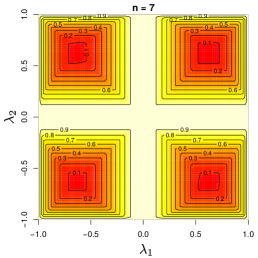
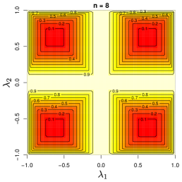
Figure 2 shows, for symmetric $\mathbf{A}$, the value of $||\mathbf{M}_{n}||_{\text{op}}$ for $n=3,\ldots,8$, and $d=2$ when the two eigenvalues of $\mathbf{A}$ range in the interval $(-1,1)$. We observe that $||\mathbf{M}_{n}||_{\text{op}}$ is always smaller than one. As described before, this will lead to a reduction in the $\ell_{2}$-norm of the cumulants in the anti-causal direction due to (11), and will in consequence produce a Gaussianization effect on the distribution of the residuals. For $n\leq 2$ it can be readily shown that $||\mathbf{M}_{1}||_{\text{op}}=||\mathbf{M}_{2}||_{\text{op}}=1$.

Figure 2: Contour curves of the values of $||\mathbf{M}_{n}||_{\text{op}}$ for $d=2$ and for $n>2$ as a function of $\lambda_{1}$ and $\lambda_{2}$, i.e., the two eigenvalues of $\mathbf{A}$. $\mathbf{A}$ is assumed to be symmetric. Similar results are obtained for higher-order cumulants.

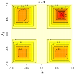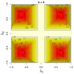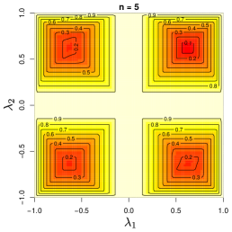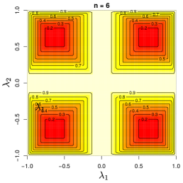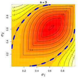
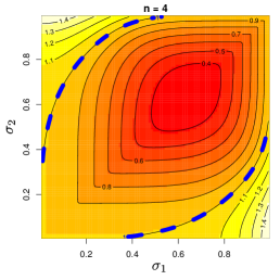
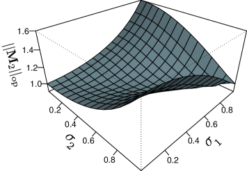
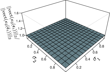
In general, the matrix $\mathbf{A}$ need not be symmetric. In this case, $||\mathbf{M}_{1}||_{\text{op}}=||\mathbf{M}_{2}||_{\text{op}}=1$ as well. However, the evaluation of $||\mathbf{M}_{n}||_{\text{op}}$ for $n>2$ is more difficult, but feasible for small $n$. Figure 3 displays the values of $||\mathbf{M}_{n}||_{\text{op}}$, for $d=2$, as the two singular values of $\mathbf{A}$, $\sigma_{1}$ and $\sigma_{2}$, vary in the interval $(0,1)$. The left singular vectors and the right singular vectors of $\mathbf{A}$ are chosen at random. In this figure a dashed blue line highlights the boundary of the region where $||\mathbf{M}_{n}||_{\text{op}}$ is strictly smaller than one. We observe that for most values of $\sigma_{1}$ and $\sigma_{2}$, $||\mathbf{M}_{n}||_{\text{op}}$ is smaller than one, leading to a Gaussianization effect in the distribution of the residuals in the anti-causal direction. However, for some singular values, $||\mathbf{M}_{n}||_{\text{op}}$ is strictly larger than one. Of course, this does not mean that there is not such a Gaussianization effect also in those cases. The definition given for $||\mathbf{M}_{n}||_{\text{op}}$ assumes that all potential vectors $\mathbf{v}$ represent valid cumulants of a probability distribution, which need not be the case in practice. For example, it is well known that cumulants exhibit some form of symmetry (McCullagh, 1987). This can be seen in the second order cumulant, which is a covariance matrix. The consequence is that $||\mathbf{M}_{n}||_{\text{op}}$ is simply an upper bound on the reduction of the $\ell_{2}$-norm of the cumulants in the anti-causal model. Thus, we also expect a Gaussianization effect to occur also for these cases. Furthermore, the numerical simulations presented in Section 6 provide evidence of this effect for asymmetric $\mathbf{A}$.

Figure 3: Contour curves of the values of $||\mathbf{M}_{n}||_{\text{op}}$ for $d=2$ and for $n>2$ as a function of $\sigma_{1}$ and $\sigma_{2}$, i.e., the two singular values of $\mathbf{A}$. $\mathbf{A}$ is not assumed to be symmetric. The singular vectors of $\mathbf{A}$ are chosen at random. A dashed blue line highlights the boundary of the region where $||\mathbf{M}_{n}||_{\text{op}}$ is strictly smaller than one.

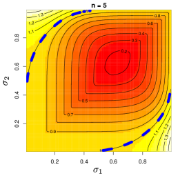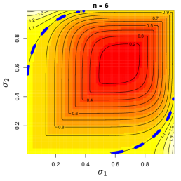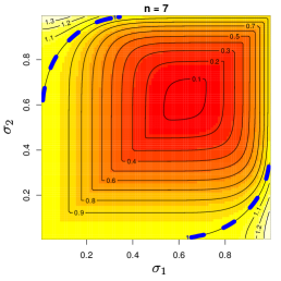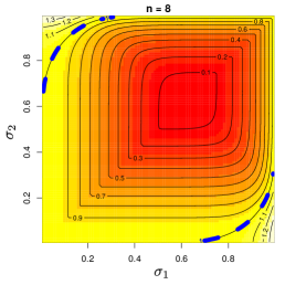The fact that $||\mathbf{M}_{n}||_{\text{op}}$ is only an upper bound is illustrated in Figure 4. This figure considers the particular case of the second cumulant $\kappa_{2}(\cdot)$, which can be analyzed in detail. On the left plot the value of $||\mathbf{M}_{2}||_{\text{op}}$ is displayed as a function of $\sigma_{1}$ and $\sigma_{2}$, the two singular values of $\mathbf{A}$. We observe that $||\mathbf{M}_{2}||_{\text{op}}$ takes values that are larger than one. In this case it is possible to evaluate in closed form the $\ell_{2}$-norm of $\text{vect}(\kappa_{2}(\bm{\epsilon}_{i}))$ and $\text{vect}(\kappa_{2}(\tilde{\bm{\epsilon}}_{i}))$, i.e., the vectors that contain the second order cumulant of the residuals in each direction. In particular, it is well known that the second order cumulant is equal to the covariance matrix (McCullagh, 1987). In the causal direction, the covariance matrix of the residuals is $\mathbf{C}=\mathbf{I}-\mathbf{A}\mathbf{A}^{\text{T}}$, as shown in the previous paragraphs. The covariance matrix of the residuals in the anti-causal direction, denoted by $\tilde{\mathbf{C}}$, can be computed similarly. Namely, $\tilde{\mathbf{C}}=\mathbf{I}-\mathbf{A}^{\text{T}}\mathbf{A}$. These two matrices, i.e., $\mathbf{C}$ and $\tilde{\mathbf{C}}$, respectively give $k_{2}(\bm{\epsilon}_{i})$ and $k_{2}(\tilde{\bm{\epsilon}}_{i})$. Furthermore, they have the same singular values. This means that $||\text{vect}(k_{2}(\bm{\epsilon}_{i}))||_{2}/||\text{vect}(k_{2}(\tilde{\bm{\epsilon}}_{i}))||_{2}=1$, as illustrated by the right plot in Figure 4. Thus, $||\mathbf{M}_{2}||_{\text{op}}$ is simply an upper bound on the actual reduction of the $\ell_{2}$-norm of the second order cumulant of the residuals in the anti-causal direction. The same behavior is expected for $||\mathbf{M}_{n}||_{\text{op}}$, with $n>2$. In consequence, one should expect that the cumulants of the distribution of the residuals of a model fitted in the anti-causal direction are smaller in magnitude. This will lead to an increased level of Gaussianity measured in terms of a reduction of the magnitude of the high-order cumulants.

Figure 4: (left) Value of $||\mathbf{M}_{2}||_{\text{op}}$, for $d=2$, as a function of $\sigma_{1}$ and $\sigma_{2}$, i.e., the two singular values of $\mathbf{A}$. (right) Actual ratio between $||\text{vect}(\kappa_{2}(\bm{\epsilon}_{i}))||_{2}$ and $||\text{vect}(\kappa_{2}(\tilde{\bm{\epsilon}}_{i}))||_{2}$, for $d=2$, as a function of $\sigma_{1}$ and $\sigma_{2}$. $\mathbf{A}$ is not assumed to be symmetric. The singular vectors of $\mathbf{A}$ are chosen at random.

2.3 Analysis of the multivariate case based on information theory

The analysis of the multivariate case carried out in the previous section is illustrative. Nevertheless, it does not prove that the distribution of the residuals in the anti-casual direction is more Gaussian based on a reduction of the magnitude of the cumulants. Further evidence of this increased level of Gaussianity can be obtained based on an increase of the entropy obtained by using information theory. In this case we also assume that the multi-dimensional variables $\mathcal{X}$ and $\mathcal{Y}$ follow the same distribution, but unlike in the previous section, they need not be whitened, only centered. In this section we closely follow (Hyvärinen and Smith, 2013, Sec. 2.4) and extend their results to the multivariate case.

Under the assumptions specified earlier, the model in the causal direction is $\mathbf{y}_{i}=\mathbf{A}\mathbf{x}_{i}+\bm{\epsilon}_{i}$, with $\mathbf{x}_{i}\bot\bm{\epsilon}_{i}$ and $\mathbf{A}=\text{Cov}(\mathcal{Y},\mathcal{X})\text{Cov}(\mathcal{X},\mathcal{X})^{-1}$. Similarly, the model in the anti-causal direction is $\mathbf{x}_{i}=\tilde{\mathbf{A}}\mathbf{y}_{i}+\tilde{\bm{\epsilon}}_{i}$ with $\tilde{\mathbf{A}}=\text{Cov}(\mathcal{X},\mathcal{Y})\text{Cov}(\mathcal{Y},\mathcal{Y})^{-1}$. By making use of the causal model it is possible to show that $\tilde{\bm{\epsilon}}_{i}=(\mathbf{I}-\tilde{\mathbf{A}}\mathbf{A})\mathbf{x}_{i}-\tilde{\mathbf{A}}\bm{\epsilon}_{i}$, where $\mathbf{I}$ is the identity matrix. Thus, the following equations are satisfied:

$$\left(\begin{array}[]{c}\mathbf{x}_{i}\\ \mathbf{y}_{i}\end{array}\right) =\mathbf{P}\left(\begin{array}[]{c}\mathbf{x}_{i}\\ \bm{\epsilon}_{i}\end{array}\right)=\left(\begin{array}[]{cc}\mathbf{I}&\mathbf{0}\\ \mathbf{A}&\mathbf{I}\end{array}\right)\left(\begin{array}[]{c}\mathbf{x}_{i}\\ \bm{\epsilon}_{i}\end{array}\right)\,,$$ (21)

and

$$\left(\begin{array}[]{c}\mathbf{y}_{i}\\ \tilde{\bm{\epsilon}}_{i}\end{array}\right) =\tilde{\mathbf{P}}\left(\begin{array}[]{c}\mathbf{x}_{i}\\ \bm{\epsilon}_{i}\end{array}\right)=\left(\begin{array}[]{cc}\mathbf{A}&\mathbf{I}\\ \mathbf{I}-\tilde{\mathbf{A}}\mathbf{A}&-\tilde{\mathbf{A}}\end{array}\right)\left(\begin{array}[]{c}\mathbf{x}_{i}\\ \bm{\epsilon}_{i}\end{array}\right)\,.$$ (30)

Let $H(\mathbf{x}_{i},\mathbf{y}_{i})$ be the entropy of the joint distribution of the two random variables associated with samples $\mathbf{x}_{i}$ and $\mathbf{y}_{i}$. Because (21) is a linear transformation, we can use the entropy transformation formula (Hyvärinen and Smith, 2013) to get that $H(\mathbf{x}_{i},\mathbf{y}_{i})$ = $H(\mathbf{x}_{i},\bm{\epsilon}_{i})+\log|\text{det}\mathbf{P}|$, where $\text{det}\mathbf{P}=\text{det}\mathbf{I}=1$. Thus, we have that $H(\mathbf{x}_{i},\mathbf{y}_{i})$ = $H(\mathbf{x}_{i},\bm{\epsilon}_{i})$. Conversely, if we use (30) we have $H(\mathbf{y}_{i},\bm{\epsilon}_{i})$ = $H(\mathbf{x}_{i},\bm{\epsilon}_{i})+\log|\text{det}\tilde{\mathbf{P}}|$, where $\text{det}\tilde{\mathbf{P}}=\text{det}\mathbf{A}\cdot\text{det}(-\tilde{\mathbf{A}}-(\mathbf{I}-\tilde{\mathbf{A}}\mathbf{A})\mathbf{A}^{-1}\mathbf{I})=-\text{det}\mathbf{I}=-1$, under the assumption that $\mathbf{A}$ is invertible. The result is that $H(\mathbf{x}_{i},\mathbf{y}_{i})=H(\mathbf{y}_{i},\bm{\epsilon}_{i})$ = $H(\mathbf{x}_{i},\bm{\epsilon}_{i})$.

Denote the mutual information between the cause and the noise with $I(\mathbf{x}_{i},\bm{\epsilon}_{i})$. Similarly, let $I(\mathbf{y}_{i},\tilde{\bm{\epsilon}}_{i})$ be the mutual information between the random variables corresponding to the observations $\mathbf{y}_{i}$ and $\tilde{\bm{\epsilon}}_{i}$. Then,

$$I(\mathbf{x}_{i},\bm{\epsilon}_{i})-I(\mathbf{y}_{i},\tilde{\bm{\epsilon}}_{i}) =H(\mathbf{x}_{i})+H(\bm{\epsilon}_{i})-H(\mathbf{x}_{i},\bm{\epsilon}_{i})-H(\mathbf{y}_{i})-H(\tilde{\bm{\epsilon}}_{i})+H(\mathbf{y}_{i},\tilde{\bm{\epsilon}}_{i})$$

$$=H(\mathbf{x}_{i})+H(\bm{\epsilon}_{i})-H(\mathbf{y}_{i})-H(\tilde{\bm{\epsilon}}_{i})\,.$$ (31)

Furthermore, from the actual causal model assumed we know that $I(\mathbf{x}_{i},\bm{\epsilon}_{i})=0$. By contrast, we have that $I(\mathbf{y}_{i},\tilde{\bm{\epsilon}}_{i})\geq 0$, since both $\mathbf{y}_{i}$ and $\tilde{\bm{\epsilon}}_{i}$ depend on $\mathbf{x}_{i}$ and $\bm{\epsilon}_{i}$. We also know that $H(\mathbf{x}_{i})=H(\mathbf{y}_{i})$ because we have made the hypothesis that both $\mathcal{X}$ and $\mathcal{Y}$ follow the same distribution. The result is that:

$$H(\bm{\epsilon}_{i})\leq H(\tilde{\bm{\epsilon}}_{i})\,,$$ (32)

with equality iff the residuals are Gaussian. We note that an alternative but equivalent way to obtain this last result is to consider a multivariate version of Lemma 1 in (Kpotufe et al., 2014), under the assumption of the same distribution for the cause and the effect. In particular, even though Kpotufe et al. (2014) assume univariate random variables, their work can be easily generalized to multiple variables.

Although the random variables corresponding to $\bm{\epsilon}_{i}$ and $\tilde{\bm{\epsilon}}_{i}$ have both zero mean, they need not have the same covariance matrix. Denote with $\text{Cov}(\bm{\epsilon}_{i})$ and $\text{Cov}(\tilde{\bm{\epsilon}}_{i})$ to these matrices and let $\hat{\bm{\epsilon}}_{i}$ and $\hat{\tilde{\bm{\epsilon}}}_{i}$ be the whitened residuals (i.e., the residuals multiplied by the Cholesky factor of the inverse of the corresponding covariance matrix). Then,

$$H(\hat{\bm{\epsilon}}_{i}) \leq H(\hat{\tilde{\bm{\epsilon}}}_{i})-\frac{1}{2}\log|\text{det}\text{Cov}(\tilde{\bm{\epsilon}}_{i})|+\frac{1}{2}\log|\text{det}\text{Cov}(\bm{\epsilon}_{i})|\,.$$ (33)

As shown in Appendix A, although not equal, the matrices $\text{Cov}(\bm{\epsilon}_{i})$ and $\text{Cov}(\tilde{\bm{\epsilon}}_{i})$ have the same determinant. Thus, the two determinants cancel in the equation above. This gives,

$$H(\hat{\bm{\epsilon}}_{i})\leq H(\hat{\tilde{\bm{\epsilon}}}_{i})\,.$$ (34)

The consequence is that the entropy of the whitened residuals in the anti-causal direction is expected to be higher or equal than the entropy of the whitened residuals in the causal direction. Because the Gaussian distribution is the continuous distribution with the highest entropy for a fixed covariance matrix, we conclude that the level of Gaussianity of the residuals in the anti-causal direction, measured in terms of differential entropy, has to be larger or equal to the level of Gaussianity of the residuals in the causal direction.

In summary, if the causal relation between the two identically distributed random variables $\mathcal{X}$ and $\mathcal{Y}$ is linear the residuals of a least squares fit in the anti-causal direction are more Gaussian than those of a linear fit in the causal direction. This Gaussianization can be characterized by a reduction of the magnitude of the corresponding high-order cumulants (although we have not formally proved this, we have provided some evidence that this is the case) and by an increase of the entropy (we have proved this in this section). A causal inference method can take advantage of this asymmetry to determine the causal direction. In particular, statistical tests based on measures of Gaussianity can be used for this purpose. However and importantly, these measures of Gaussianity need not be estimates of the differential entropy or the high-order cumulants. In particular, the entropy is a quantity that is particularly difficult to estimate in practice (Beirlant et al., 1997). The same occurs with the high-order cumulants. Their estimators involve high-order moments, and hence suffer from high variance.

When the distribution of the residuals in (6) is Gaussian, the causal direction cannot be identified. In this case, it is possible to show that the distribution of the reversed residuals $\tilde{\bm{\epsilon}}_{i}$, the cause $\mathbf{x}_{i}$, and the effect $\mathbf{y}_{i}$, is Gaussian as a consequence of (9) and (11). This non-identifiability agrees with the general result of Shimizu et al. (2006), which indicates that non-Gaussian distributions are strictly required in the disturbance variables to carry out causal inference in linear models with additive independent noise.

Finally, the fact that the Gaussianization effect is also expected in the multivariate case suggests a method to address causal inference problems in which the relationship between cause and effect is non-linear: It consists in mapping each observation $x_{i}$ and $y_{i}$ to a vector in an expanded feature space. One can them assume that the non-linear relation in the original input space is linear in the expanded feature space and compute the residuals of kernel ridge regressions in both directions. The direction in which the residuals are less Gaussian is identified as the causal one.

3 A feature expansion to address non-linear causal inference problems

We now proceed to relax the assumption that the causal relationship between the unidimensional random variables $\mathcal{X}$ and $\mathcal{Y}$ is linear. For this purpose, instead of working in the original space in which the samples $\left\{(x_{i},y_{i})\right\}_{i=1}^{N}$ are observed, we will assume that the model is linear in some expanded feature space $\left\{\left(\phi(x_{i}),\phi(y_{i})\right)\right\}_{i=1}^{N}$ for some mapping function $\phi(\cdot):\mathds{R}\rightarrow\mathds{R}^{d}$. Importantly, this map preserves the property that if $x_{i}$ and $y_{i}$ are equally distributed, so will be $\phi(x_{i})$ and $\phi(y_{i})$. According to the analysis presented in the previous section, the residuals of a linear model in the expanded space should be more Gaussian in the anti-causal direction than the residuals of a linear model in the causal direction, based on an increment of the differential entropy and on a reduction of the magnitude of the cumulants. The assumption we make is that the non-linear relation between $\mathcal{X}$ and $\mathcal{Y}$ in the original input space is linear in the expanded feature space.

In this section we focus on obtaining the normalized residuals of linear models formulated in the expanded feature space. For this purpose, we assume that a kernel function $k(\cdot,\cdot)$ can be used to evaluate dot products in the expanded feature space. In particular, $k(x_{i},x_{j})=\phi(x_{i})^{\text{T}}\phi(x_{j})$ and $k(y_{i},y_{j})=\phi(y_{i})^{\text{T}}\phi(y_{j})$ for arbitrary $x_{i}$ and $x_{j}$ and $y_{i}$ and $y_{j}$. Furthermore, we will not assume in general that $\phi(x_{i})$ and $\phi(y_{i})$ have been whitened, only centered. Whitening is a linear transformation which is not expected to affect to the level of Gaussianity of the residuals. However, once these residuals have been obtained they will be whitened in the expanded feature space. Later on we describe how to center the data in the expanded feature space. For now on, we will assume this step has already been done.

3.1 Non-linear model description and fitting process

Assume that the relation between $\mathcal{X}$ and $\mathcal{Y}$ is linear in an expanded feature space

$$\phi(y_{i})=\mathbf{A}\phi(x_{i})+\bm{\epsilon}_{i}\,,\quad\bm{\epsilon}_{i}\perp x_{i},$$ (35)

where $\bm{\epsilon}_{i}$ is i.i.d. non-Gaussian additive noise.

Given $N$ paired observations $\{(x_{i},y_{i})\}_{i=1}^{N}$ drawn i.i.d. from $P(\mathcal{X},\mathcal{Y})$, define the matrices $\bm{\Phi}_{x}=(\phi(x_{1}),\ldots,\phi(x_{N}))$ and $\bm{\Phi}_{y}=(\phi(y_{1}),\ldots,\phi(y_{N}))$ of size $d\times N$. The estimate of $\mathbf{A}$ that minimizes the sum of squared errors is $\hat{\mathbf{A}}=\bm{\Gamma}\bm{\Sigma}^{-1}$, where $\bm{\Gamma}=\bm{\Phi}_{y}\bm{\Phi}_{x}^{\text{T}}$ and $\bm{\Sigma}=\bm{\Phi}_{x}\bm{\Phi}_{x}^{\text{T}}$. Unfortunately, when $d>N$, where $d$ is the number of variables in the feature expansion, the matrix $\bm{\Sigma}^{-1}$ does not exist and $\hat{\mathbf{A}}$ is not unique. This means that there is an infinite number of solutions for $\hat{\mathbf{A}}$ with zero squared error.

To avoid the indetermination described above and also to alleviate over-fitting, we propose a regularized estimator. Namely,

$$\mathcal{L}(\mathbf{A}) =\sum_{i=1}^{N}\frac{1}{2}||\phi(y_{i})-\mathbf{A}\phi(x_{i})||_{2}^{2}+\tau\frac{1}{2}||\mathbf{A}||_{\mathcal{F}}^{2}\,,$$ (36)

where $||\cdot||_{2}$ denotes the $\ell_{2}$-norm and $||\cdot||_{\mathcal{F}}$ denotes the Frobenius norm. In this last expression $\tau>0$ is a parameter that controls the amount of regularization. The minimizer of (36) is $\hat{\mathbf{A}}=\bm{\Gamma}\bm{\Sigma}^{-1}$, where $\bm{\Gamma}=\bm{\Phi}_{y}\bm{\Phi}_{x}^{\text{T}}$ and $\bm{\Sigma}=\tau\mathbf{I}+\bm{\Phi}_{x}\bm{\Phi}_{x}^{\text{T}}$. The larger the value of $\tau$, the closer the entries of $\hat{\mathbf{A}}$ are to zero. Furthermore, using the matrix inversion lemma we have that $\bm{\Sigma}^{-1}=\tau^{-1}\mathbf{I}-\tau^{-1}\bm{\Phi}_{x}\mathbf{V}^{-1}\bm{\Phi}_{x}^{\text{T}}$, where $\mathbf{V}=\left(\tau\mathbf{I}+\mathbf{K}_{x,x}\right)^{-1}$ and $\mathbf{K}_{x,x}=\bm{\Phi}_{x}^{\text{T}}\bm{\Phi}_{x}$ is a kernel matrix whose entries are given by $k(x_{i},x_{j})$. After some algebra it is possible to show that

$$\hat{\mathbf{A}} =\bm{\Gamma}\bm{\Sigma}^{-1}=\bm{\Phi}_{y}\mathbf{V}\bm{\Phi}_{x}^{\text{T}}\,,$$ (37)

which depends only on the matrix $\mathbf{V}$. This matrix be computed with cost $\mathcal{O}(N^{3})$. We note that the estimate obtained in (37) coincides with the kernel conditional embedding operator described by Song et al. (2013) for mapping conditional distributions into infinite dimensional feature spaces using kernels.

3.2 Obtaining the matrix of inner products of the residuals

A first step towards obtaining the whitened residuals in feature space (which will be required for the estimation of their level of Gaussianity) is to compute the matrix of inner products of these residuals (kernel matrix). For this, we define $\bm{\epsilon}_{i}=\phi(y_{i})-\hat{\mathbf{A}}\phi(x_{i})$. Thus,

$$\bm{\epsilon}_{i}^{\text{T}}\bm{\epsilon}_{j} =\left[\phi(y_{i})-\hat{\mathbf{A}}\phi(x_{i})\right]^{\text{T}}\left[\phi(y_{j})-\hat{\mathbf{A}}\phi(x_{j})\right]$$

$$=\phi(y_{i})^{\text{T}}\phi(y_{j})-\phi(y_{i})^{\text{T}}\hat{\mathbf{A}}\phi(x_{j})-\phi(x_{i})^{\text{T}}\hat{\mathbf{A}}\phi(y_{j})+\phi(x_{i})^{\text{T}}\hat{\mathbf{A}}\hat{\mathbf{A}}\phi(x_{j})\,,$$ (38)

for two arbitrary residuals $\bm{\epsilon}_{i}$ and $\bm{\epsilon}_{j}$ in feature space. In general, if we denote with $\mathbf{K}_{\epsilon}$ to the matrix whose entries are given by $\bm{\epsilon}_{i}^{\text{T}}\bm{\epsilon}_{j}$ and define $\mathbf{K}_{y,y}=\bm{\Phi}_{y}^{\text{T}}\bm{\Phi}_{y}$, we have that

$$\mathbf{K}_{\epsilon} =\mathbf{K}_{y,y}-\mathbf{K}_{y,y}\mathbf{V}\mathbf{K}_{x,x}-\mathbf{K}_{x,x}\mathbf{V}\mathbf{K}_{y,y}+\mathbf{K}_{x,x}\mathbf{V}\mathbf{K}_{y,y}\mathbf{V}\mathbf{K}_{x,x}\,,$$ (39)

where we have used the definition of $\hat{\mathbf{A}}$ in (37). This expression only depends on the kernel matrices $\mathbf{K}_{x,x}$ and $\mathbf{K}_{y,y}$ and the matrix $\mathbf{V}$, and can be computed with cost $\mathcal{O}(N^{3})$.

3.3 Centering the input data and centering and whitening the residuals

An assumption made in Section 2 was that the samples of the random variables $\mathcal{X}$ and $\mathcal{Y}$ are centered, i.e., they have zero mean. In this section we show how to carry out this centering process in feature space. Furthermore, we also show how to center the residuals of the fitting process, which are also whitened. Whitening is a standard procedure in which the data are transformed to have the identity matrix as the covariance matrix. It also corresponds to projecting the data onto all the principal components, and scaling them to have unit standard deviation.

We show how to center the data in feature space. For this, we follow (Schölkopf et al., 1997) and work with:

$$\tilde{\phi}(x_{i}) =\phi(x_{i})-\frac{1}{N}\sum_{j=1}^{N}\phi(x_{j})\,, \tilde{\phi}(y_{i}) =\phi(y_{i})-\frac{1}{N}\sum_{j=1}^{N}\phi(y_{j})\,.$$ (40)

The consequence is that now the kernel matrices $\mathbf{K}_{x,x}$ and $\mathbf{K}_{y,y}$ are replaced by

$$\tilde{\mathbf{K}}_{x,x} =\mathbf{K}_{x,x}-\mathbf{1}_{N}\mathbf{K}_{x,x}-\mathbf{K}_{x,x}\mathbf{1}_{N}+\mathbf{1}_{N}\mathbf{K}_{x,x}\mathbf{1}_{N}\,,$$

$$\tilde{\mathbf{K}}_{y,y} =\mathbf{K}_{y,y}-\mathbf{1}_{N}\mathbf{K}_{y,y}-\mathbf{K}_{y,y}\mathbf{1}_{N}+\mathbf{1}_{N}\mathbf{K}_{y,y}\mathbf{1}_{N}\,,$$ (41)

where $\mathbf{1}_{N}$ is a $N\times N$ matrix with all entries equal to $1/N$. The residuals can be centered also in a similar way. Namely, $\tilde{\mathbf{K}}_{\epsilon}=\mathbf{K}_{\epsilon}-\mathbf{1}_{N}\mathbf{K}_{\epsilon}-\mathbf{K}_{\epsilon}\mathbf{1}_{N}+\mathbf{1}_{N}\mathbf{K}_{\epsilon}\mathbf{1}_{N}$.

We now explain the whitening of the residuals, which are now assumed to be centered. This process involves the computation of the eigenvalues and eigenvectors of the $d\times d$ covariance matrix $\mathbf{C}$ of the residuals. This is done as in kernel PCA (Schölkopf et al., 1997). Denote by $\tilde{\bm{\epsilon}}_{i}$ to the centered residuals. The covariance matrix is $\mathbf{C}=N^{-1}\sum_{i=1}^{N}\tilde{\bm{\epsilon}}_{i}\tilde{\bm{\epsilon}}_{i}^{\text{T}}$. The eigenvector expansion implies that $\mathbf{C}\mathbf{v}_{i}=\lambda_{i}\mathbf{v}_{i}$, where $\mathbf{v}_{i}$ denotes the $i$-th eigenvector and $\lambda_{i}$ the $i$-th eigenvalue. The consequence is that $N^{-1}\sum_{k=1}^{N}\tilde{\bm{\epsilon}}_{k}\tilde{\bm{\epsilon}}_{k}^{\text{T}}\mathbf{v}_{i}=\lambda_{i}\mathbf{v}_{i}$. Thus, the eigenvectors can be expressed as a combination of the residuals. Namely, $\mathbf{v}_{i}=\sum_{j=1}^{N}b_{i,j}\tilde{\bm{\epsilon}}_{j}$, where $b_{i,j}=N^{-1}\tilde{\bm{\epsilon}}_{j}^{\text{T}}\mathbf{v}_{i}$. Substituting this result in the previous equation we have that $N^{-1}\sum_{k=1}^{N}\tilde{\bm{\epsilon}}_{k}\tilde{\bm{\epsilon}}_{k}^{\text{T}}\sum_{j=1}^{N}b_{i,j}\tilde{\bm{\epsilon}}_{j}=\lambda_{i}\sum_{j=1}^{N}b_{i,j}\tilde{\bm{\epsilon}}_{j}$. When we multiply both sides by $\tilde{\bm{\epsilon}}_{l}^{\text{T}}$ we obtain $N^{-1}\sum_{k=1}^{N}\tilde{\bm{\epsilon}}_{l}^{\text{T}}\tilde{\bm{\epsilon}}_{k}\tilde{\bm{\epsilon}}_{k}^{\text{T}}\sum_{j=1}^{N}b_{i,j}\tilde{\bm{\epsilon}}_{j}=\lambda_{i}\sum_{j=1}^{N}b_{i,j}\tilde{\bm{\epsilon}}_{l}^{\text{T}}\tilde{\bm{\epsilon}}_{j}$, for $l=1,\ldots d$, which is written in terms of kernels as $\tilde{\mathbf{K}}_{\epsilon}\tilde{\mathbf{K}}_{\epsilon}\mathbf{b}_{i}=\lambda_{i}N\tilde{\mathbf{K}}_{\epsilon}\mathbf{b}_{i}$, where $\mathbf{b}_{i}=(b_{i,1},\ldots,b_{i,N})^{\text{T}}$. A solution to this problem is found by solving the eigenvalue problem $\tilde{\mathbf{K}}_{\epsilon}\mathbf{b}_{i}=\lambda_{i}N\mathbf{b}_{i}$. We also require that the eigenvectors have unit norm. Thus, $1=\mathbf{v}_{i}^{\text{T}}\mathbf{v}_{i}=\sum_{j=1}^{N}\sum_{k=1}^{N}b_{i,j}b_{i,k}\tilde{\bm{\epsilon}}_{j}^{\text{T}}\tilde{\bm{\epsilon}}_{k}=\mathbf{b}_{i}^{\text{T}}\tilde{\mathbf{K}}_{\epsilon}\mathbf{b}_{i}=\lambda_{i}N\mathbf{b}_{i}^{\text{T}}\mathbf{b}_{i}$, which means that $\mathbf{b}_{i}$ has norm $1/\sqrt{\lambda_{i}N}$. Consider now that $\tilde{\mathbf{b}}_{i}$ is one eigenvector of $\tilde{\mathbf{K}}_{\epsilon}$. Then, $\mathbf{b}_{i}=1/\sqrt{\lambda_{i}N}\tilde{\mathbf{b}}_{i}$. Similarly, let $\tilde{\lambda}_{i}$ be an eigenvalue of $\tilde{\mathbf{K}}_{\epsilon}$. Then $\lambda_{i}=\tilde{\lambda}_{i}/N$. In summary, $\lambda_{i}$ and $b_{i,j}$, with $i=1,\ldots,N$ and $j=1,\ldots,N$ can be found with cost $\mathcal{O}(N^{3})$ by finding the eigendecomposition of $\tilde{\mathbf{K}}_{\epsilon}$.

The whitening process is carried out by projecting each residual $\tilde{\bm{\epsilon}}_{k}$ onto each eigenvector $\mathbf{v}_{i}$ and then multiplying by $1/\sqrt{\lambda_{i}}$. The corresponding $i$-th component for the $k$-th residual, denoted by $Z_{k,i}$, is $Z_{k,i}=1/\sqrt{\lambda_{i}}\mathbf{v}_{i}^{\text{T}}\tilde{\bm{\epsilon}}_{k}=1/\sqrt{\lambda_{i}}\sum_{j=1}^{N}b_{i,j}\tilde{\bm{\epsilon}}_{j}^{\text{T}}\tilde{\bm{\epsilon}}_{k}$, and in consequence, the whitened residuals are $\mathbf{Z}=\tilde{\mathbf{K}}_{\epsilon}\mathbf{B}\mathbf{D}=N\mathbf{B}\mathbf{D}^{-1}=\sqrt{N}\tilde{\mathbf{B}}$, where $\mathbf{B}$ is a matrix whose columns contain each $\mathbf{b}_{i}$, $\tilde{\mathbf{B}}$ is a matrix whose columns contain each $\tilde{b}_{i}$ and $\mathbf{D}$ is a diagonal matrix whose entries are equal to $1/\sqrt{\lambda_{i}}$. Each row of $\mathbf{Z}$ now contains the whitened residuals.

3.4 Inferring the most likely causal direction

After having trained the model and obtained the matrix of whitened residuals $\mathbf{Z}$ in each direction, a suitable Gaussianity test can be used to determine the correct causal relation between the variables $\mathcal{X}$ and $\mathcal{Y}$. Given the theoretical results of Section 2 one may be tempted to use tests based on entropy or cumulants estimation. Such tests may perform poorly in practice due to the difficulty of estimating high-order cumulants or differential entropy. In particular, the estimators of the cumulants involve high-order moments and hence, suffer from high variance. As a consequence, in our experiments we use a statistical test for Gaussianity based on the energy distance (Székely and Rizzo, 2005), which has good power, is robust to noise, and does not have any adjustable hyper-parameters. Furthermore, in Appendix B we motivate that in the anti-causal direction one should also expect a smaller energy distance to the Gaussian distribution.

Assume $\mathcal{X}$ and $\mathcal{Y}$ are two independent random variables whose probability distribution functions are $F(\cdot)$ and $G(\cdot)$. The energy distance between these distributions is defined as

$$D^{2}(F,G) =2\mathds{E}[||\mathcal{X}-\mathcal{Y}||]-\mathds{E}[||\mathcal{X}-\mathcal{X}^{\prime}||]-\mathds{E}[||\mathcal{Y}-\mathcal{Y}^{\prime}||]\,,$$ (42)

where $||\cdot||$ denotes some norm, typically the $\ell_{2}$-norm; $\mathcal{X}$ and $\mathcal{X}^{\prime}$ are independent and identically distributed (i.i.d.); $\mathcal{Y}$ and $\mathcal{Y}^{\prime}$ are i.i.d; and $\mathds{E}$ denotes expected value. The energy distance satisfies all axioms of a metric and hence characterizes the equality of distributions. Namely, $D^{2}(F,G)=0$ if and only if $F=G$. Furthermore, in the case of univariate random variables the energy distance is twice the Cramér-von Mises distance given by $\int\left(F(x)-G(x)\right)^{2}dx$.

Assume $\mathbf{X}=(\mathbf{x}_{1},\ldots,\mathbf{x}_{N})^{\text{T}}$ is a matrix that contains $N$ random samples (one per each row of the matrix) from a $d$ dimensional random variable with probability density $f$. The statistic described for testing for Gaussianity, i.e., $\text{H}_{0}:f=\mathcal{N}(\cdot|\mathbf{0},\mathbf{I})$ vs $\text{H}_{1}:f\neq\mathcal{N}(\cdot|\mathbf{0},\mathbf{I})$, that is described in (Székely and Rizzo, 2005) is:

$$\text{Energy}(\mathbf{X}) =N\left(\frac{2}{N}\sum_{j=1}^{N}\mathds{E}[||\mathbf{x}_{j}-\mathcal{Y}||]-\mathds{E}[||\mathcal{Y}-\mathcal{Y}^{\prime}||]-\frac{1}{N^{2}}\sum_{j,k=1}^{N}||\mathbf{x}_{j}-\mathbf{x}_{k}||\right)\,,$$ (43)

where $\mathcal{Y}$ and $\mathcal{Y}^{\prime}$ are independent random variables distributed as $\mathcal{N}(\cdot|\mathbf{0},\mathbf{I})$ and $\mathds{E}$ denotes expected value. Furthermore, the required expectations with respect to the Gaussian random variables $\mathcal{Y}$ and $\mathcal{Y}^{\prime}$ can be efficiently computed as described in (Székely and Rizzo, 2005). The idea is that if $f$ is similar to a Gaussian density $\mathcal{N}(\cdot|0,\mathbf{I})$, then $\text{Energy}(\mathbf{X})$ is close to zero. Conversely, the null hypothesis $H_{0}$ is rejected for large values of $\text{Energy}(\mathbf{X})$.

The data to test for Gaussianity is in our case $\mathbf{Z}$, i.e., the matrix of whitened residuals, which has size $N\times N$. Thus, the whitened residuals have $N$ dimensions. The direct introduction of these residuals into a statistical test for Gaussianity is not expected to provide meaningful results, as a consequence of the high dimensionality. Furthermore, in our experiments we have observed that it is often the case that a large part of the total variance is explained by the first principal component (see the supplementary material for evidence supporting this). That is, $\lambda_{i}$, i.e., the eigenvalue associated to the $i$-th principal component, is almost negligible for $i\geq 2$. Additionally, we motivate in Appendix C that one should also obtain more Gaussian residuals, after projecting the data onto the first principal component, in terms of a reduction of the magnitude of the high-order cumulants. Thus, in practice, we consider only the first principal component of the estimated residuals in feature space. This is the component $i$ with the largest associated eigenvalue $\lambda_{i}$. We denote such $N$-dimensional vector by $\mathbf{z}$.

Let $\mathbf{z}_{x\rightarrow y}$ be the vector of coefficients of the first principal component of the residuals in feature space when the linear fit is performed in the direction $\mathcal{X}\rightarrow\mathcal{Y}$. Let $\mathbf{z}_{y\rightarrow x}$ be the vector of coefficients of the first principal component of the residuals in feature space when the linear fit is carried out in the direction $\mathcal{Y}\rightarrow\mathcal{X}$. We define the measure of Gaussianization of the residuals as $\mathcal{G}=\text{Energy}(\mathbf{z}_{x\rightarrow y})/N-\text{Energy}(\mathbf{z}_{y\rightarrow x})/N$, where $\text{Energy}(\cdot)$ computes the statistic of the energy distance test for Gaussianity described above. Note that we divide each statistic by $N$ to cancel the corresponding factor that is considered in (43). Since in this test larger values for the statistic corresponds to larger deviations from Gaussianity, if $\mathcal{G}>0$ the direction $\mathcal{X}\rightarrow\mathcal{Y}$ is expected to be more likely the causal direction. Otherwise, the direction $\mathcal{Y}\rightarrow\mathcal{X}$ is preferred.

The variance of $\mathcal{G}$ will depend on the sample size $N$. Thus, ideally one should use the difference between the $p$-values associated to each statistic as the confidence in the decision taken. Unfortunately, computing these $p$-values is expensive since the distribution of the statistic under the null hypothesis must be approximated via random sampling. In our experiments we measure the confidence of the decision in terms of the absolute value of $\mathcal{G}$, which is faster to obtain and we have found to perform well in practice.

3.5 Parameter tuning and error evaluation

Assume that a squared exponential kernel is employed in the method described above. This means that $k(x_{i},x_{j})=\exp\left(-\gamma(x_{i}-x_{j})^{2}\right)$, where $\gamma>0$ is the bandwidth of the kernel. The same is assumed for $k(y_{i},y_{j})$. Therefore, two hyper-parameters require adjustment in the method described. These are the ridge regression regularization parameter $\tau$ and the kernel bandwidth $\gamma$. They must be tuned in some way to produce the best possible fit in each direction. The method chosen to guarantee this is a grid search guided by a 10-fold cross-validation procedure, which requires computing the squared prediction error over unseen data. In this section we detail how to evaluate these errors.

Assume that $M$ new paired data instances are available for validation. Let the two matrices $\bm{\Phi}_{y^{\text{new}}}=(\phi(y_{1}^{\text{new}}),\ldots,\phi(y_{M}^{\text{new}}))$ and $\bm{\Phi}_{x^{\text{new}}}=(\phi(x_{1}^{\text{new}}),\ldots,\phi(x_{M}^{\text{new}}))$ summarize these data. Define $\bm{\epsilon}_{i}^{\text{new}}=\phi(y_{i}^{\text{new}})-\hat{\mathbf{A}}\phi(x_{i}^{\text{new}})$. After some algebra, it is possible to show that the sum of squared errors for the new instances is:

$$E=\sum_{i=1}^{M}(\bm{\epsilon}_{i}^{\text{new}})^{\text{T}}\bm{\epsilon}_{i}^{\text{new}} =\text{trace}\bigg{(}\mathbf{K}_{y^{\text{new}},y^{\text{new}}}-\mathbf{K}_{y^{\text{new}},y}\mathbf{V}\mathbf{K}_{x^{\text{new}},x}^{\text{T}}-$$

$$\quad\mathbf{K}_{x^{\text{new}},x}\mathbf{V}\mathbf{K}_{y^{\text{new}},y}^{\text{T}}+\mathbf{K}_{x^{\text{new}},x}\mathbf{V}\mathbf{K}_{y,y}\mathbf{V}\mathbf{K}_{x^{\text{new}},x}^{\text{T}}\bigg{)}\,.$$ (44)

where $\mathbf{K}_{y^{\text{new}},y^{\text{new}}}=\bm{\Phi}_{y^{\text{new}}}^{\text{T}}\bm{\Phi}_{y^{\text{new}}}$, $\mathbf{K}_{y^{\text{new}},y}=\bm{\Phi}_{y^{\text{new}}}^{\text{T}}\bm{\Phi}_{y}$ and $\mathbf{K}_{x,x^{\text{new}}}=\bm{\Phi}_{x}^{\text{T}}\bm{\Phi}_{x^{\text{new}}}$.

Of course, the new data must be centered before computing the error estimate. This process is similar to the one described in the previous section. In particular, centering can be simply carried out by working with the modified kernel matrices:

$$\tilde{\mathbf{K}}_{x^{\text{new}},x} =\mathbf{K}_{x^{\text{new}},x}-\mathbf{M}_{N}\mathbf{K}_{x,x}-\mathbf{K}_{x^{\text{new}},x}\mathbf{1}_{N}+\mathbf{M}_{N}\mathbf{K}_{x,x}\mathbf{1}_{N}\,,$$

$$\tilde{\mathbf{K}}_{y^{\text{new}},y} =\mathbf{K}_{y^{\text{new}},y}-\mathbf{M}_{N}\mathbf{K}_{y,y}-\mathbf{K}_{y^{\text{new}},y}\mathbf{1}_{N}+\mathbf{M}_{N}\mathbf{K}_{y,y}\mathbf{1}_{N}\,,$$

$$\tilde{\mathbf{K}}_{y^{\text{new}},y^{\text{new}}} =\mathbf{K}_{y^{\text{new}},y^{\text{new}}}-\mathbf{M}_{N}\mathbf{K}_{y,y^{\text{new}}}-\mathbf{K}_{y^{\text{new}},y}\mathbf{M}_{N}^{\text{T}}+\mathbf{M}_{N}\mathbf{K}_{y,y}\mathbf{M}_{N}^{\text{T}}\,,$$ (45)

where $\mathbf{M}_{N}$ is a matrix of size $M\times N$ with all components equal to $1/N$. In this process, the averages employed for the centering step are computed using only the observed data.

A disadvantage of the squared error is that it strongly depends on the kernel bandwidth parameter $\gamma$. This makes it difficult to choose this hyper-parameter in terms of such a performance measure. A better approach is to choose both $\gamma$ and $\tau$ in terms of the explained variance by the model. This is obtained as follows: $\text{Explained-Variance}=1-\text{E}/M\text{Var}_{\text{ynew}}$, where $E$ denotes the squared prediction error and $\text{Var}_{\text{ynew}}$ the variance of the targets. The computation of the error $E$ is done as described previously and $\text{Var}_{\text{ynew}}$ is simply the average of the diagonal entries in $\tilde{\mathbf{K}}_{y^{\text{new}},y^{\text{new}}}$.

3.6 Finding pre-images for illustrative purposes

The kernel method described above expresses its solution as feature maps of the original data points. Since the feature map $\phi(\cdot)$ is usually non-linear, we cannot guarantee the existence of a pre-image under $\phi(\cdot)$. That is, a point $y$ such that $\phi(y)=\hat{\mathbf{A}}\phi(x)$, for some input point $x$. An alternative to amend this issue is to find approximate pre-images, which can be useful to make predictions or plotting results (Schölkopf and Smola, 2002). In this section we describe how to find this approximate pre-images.

Assume that we have a new data instance $x_{\text{new}}$ for which we would like to know the associated target value $y_{\text{new}}$, after our kernel model has been fitted. The predicted value in feature space is:

$$\phi(y_{\text{new}}) =\bm{\Phi}_{y}\mathbf{V}\bm{\Phi}_{x}^{\text{T}}\phi(x_{\text{new}})=\bm{\Phi}_{y}\mathbf{V}\mathbf{k}_{x,x_{\text{new}}}=\sum_{i=1}^{n}\alpha_{i}\phi(y_{i})\,,$$ (46)

where $\mathbf{k}_{x,x_{\text{new}}}$ contains the kernel evaluations between each entry in $\mathbf{x}$ (i.e., the observed samples of the random variable $\mathcal{X}$) and the new instance. Finally, each $\alpha_{i}$ is given by a component of the vector $\mathbf{V}\mathbf{k}_{x,x_{\text{new}}}$. The approximate pre-image of $\phi(y_{\text{new}})$, $y_{\text{new}}$, is found by solving the following optimization problem:

$$y_{\text{new}} =\underset{u}{\text{arg min}}\quad||\phi(y_{\text{new}})-\phi(u)||^{2}_{2}=\underset{u}{\text{arg min}}\quad-2\bm{\alpha}^{\text{T}}\mathbf{k}_{y,u}+k(u,u)\,,$$ (47)

where $\mathbf{k}_{y,u}$ is a vector with the kernel values between each $y_{i}$ and $u$, and $k(u,u)=\phi(u)^{\text{T}}\phi(u)$. This is a non-linear optimization problem than can be solved approximately using standard techniques such as gradient descent. In particular, the computation of the gradient of $\mathbf{k}_{y,u}$ with respect to $u$ is very simple in the case of the squared exponential kernel.

4 Data transformation and detailed causal inference algorithm

The method for causal inference described in the previous section relies on the fact that both random variables $\mathcal{X}$ and $\mathcal{Y}$ are equally distributed. In particular, if this is the case, $\phi(x_{i})$ and $\phi(y_{i})$, i.e., the maps of $x_{i}$ and $y_{i}$ in the expanded feature space, will also be equally distributed. This means that under such circumstances one should expect residuals that are more Gaussian in the anti-causal direction due to a reduction of the magnitude of the high order cumulants and an increment of the differential entropy. The requirement that $\mathcal{X}$ and $\mathcal{Y}$ are equally distributed can be easily fulfilled in the case of continuous univariate data by transforming $\mathbf{x}$, the samples of $\mathcal{X}$, to have the same empirical distribution as $\mathbf{y}$, the samples of $\mathcal{Y}$.

Consider $\mathbf{x}=(x_{1},\ldots,x_{N})^{\text{T}}$ and $\mathbf{y}=(y_{1},\ldots,y_{N})^{\text{T}}$ to be $N$ paired samples of $\mathcal{X}$ and $\mathcal{Y}$, respectively. To guarantee the same distribution for these samples we only have to replace $\mathbf{x}$ by $\tilde{\mathbf{x}}$, where each component of $\tilde{\mathbf{x}}$, $\tilde{x}_{i}$, is given by $\tilde{x}_{i}=\hat{F}^{-1}_{y}(\hat{F}_{x}(x_{i}))$, with $\hat{F}_{y}^{-1}(\cdot)$ the empirical quantile distribution function of the random variable $\mathcal{Y}$, estimated using $\mathbf{y}$. Similarly, $\hat{F}_{x}(\cdot)$ is the empirical cumulative distribution function of $\mathcal{X}$, estimated using $\mathbf{x}$. This operation is known as the probability integral transform.

One may wonder why should $\mathbf{x}$ be transformed instead of $\mathbf{y}$. The reason is that by transforming $\mathbf{x}$ the additive noise hypothesis made in (1) and (6) is preserved. In particular, we have that $y_{i}=f(\hat{F}^{-1}_{x}(\hat{F}_{y}(\tilde{x}_{i})))+\epsilon_{i}$. On the other hand, if $\mathbf{y}$ is transformed instead, the additive noise model will generally not be valid anymore. More precisely, the transformation that computes $\tilde{\mathbf{y}}$ in such a way that it is distributed as $\mathbf{x}$ is $\tilde{y}_{i}=\hat{F}^{-1}_{x}(\hat{F}_{y}(y_{i}))$, $\forall i$. Thus, under this transformation we have that $\tilde{y}_{i}=\hat{F}^{-1}_{x}(\hat{F}_{y}(f(x_{i})+\epsilon_{i}))$, which will lead to the violation of the additive noise model.

Of course, transforming $\mathbf{x}$ requires the knowledge of the causal direction. In practice, we will transform both $\mathbf{x}$ and $\mathbf{y}$ and consider that the correct transformation is the one that leads to the highest level of Gaussianization of the residuals in the feature space, after fitting the model in each direction. That is, the transformation that leads to the highest value of $\mathcal{G}$ is expected to be the correct one. We expect that when $\mathbf{y}$ is transformed instead of $\mathbf{x}$, the Gaussianization effect of the residuals is not as high as when $\mathbf{x}$ is transformed, as a consequence of the violation of the additive noise model. This will allow to determine the causal direction. We do not have a theoretical result confirming this statement, but the good results obtained in Section 6.1 indicate that this is the case.

The details of the complete causal inference algorithm proposed are given in Algorithm 1. Besides a causal direction, e.g., $\mathcal{X}\rightarrow\mathcal{Y}$ or $\mathcal{Y}\rightarrow\mathcal{X}$, this algorithm also outputs a confidence level in the decision made which is defined as $\text{max}(|\mathcal{G}_{\tilde{x}}|,|\mathcal{G}_{\tilde{y}}|)$, where $\mathcal{G}_{\tilde{x}}=\text{Energy}(\mathbf{z}_{\tilde{x}\rightarrow y})/N-\text{Energy}(\mathbf{z}_{y\rightarrow\tilde{x}})/N$ denotes the estimated level of Gaussianization of the residuals when $\mathbf{x}$ is transformed to have the same distribution as $\mathbf{y}$. Similarly, $\mathcal{G}_{\tilde{y}}=\text{Energy}(\mathbf{z}_{\tilde{y}\rightarrow x})/N-\text{Energy}(\mathbf{z}_{\tilde{y}\rightarrow x})/N$ denotes the estimated level of Gaussianization of the residuals when $\mathbf{x}$ and $\mathbf{y}$ are swapped and $\mathbf{y}$ is transformed to have the same distribution as $\mathbf{x}$. Here $\mathbf{z}_{\tilde{x}\rightarrow y}$ contains the first principal component of the residuals in the expanded feature space when trying to predict $\mathbf{y}$ using $\tilde{\mathbf{x}}$. The same applies for $\mathbf{z}_{y\rightarrow\tilde{x}}$, $\mathbf{z}_{\tilde{y}\rightarrow x}$ and $\mathbf{z}_{x\rightarrow\tilde{y}}$. However, the residuals are obtained this time when trying to predict $\tilde{\mathbf{x}}$ using $\mathbf{y}$, when trying to predict $\mathbf{x}$ using $\tilde{\mathbf{y}}$ and when trying to predict $\tilde{\mathbf{y}}$ using $\mathbf{x}$, respectively. Recall that the reason for keeping only the first principal component of the residuals is described in Section 3.4.

Assume $|\mathcal{G}_{\tilde{x}}|>|\mathcal{G}_{\tilde{y}}|$. In this case we prefer the transformation of $\mathbf{x}$ to guarantee that the cause and the effect have the same distribution. The reason is that it leads to a higher level of Gaussianization of the residuals, as estimated by the energy statistical test. Now consider that $\mathcal{G}_{\tilde{x}}>0$. We prefer the direction $\mathcal{X}\rightarrow\mathcal{Y}$ because the residuals of a fit in that direction are less Gaussian and hence have a higher value of the statistic of the energy test. By contrast, if $\mathcal{G}_{\tilde{x}}<0$ we prefer the direction $\mathcal{Y}\rightarrow\mathcal{X}$ for the same reason. In the case that $|\mathcal{G}_{\tilde{x}}|<|\mathcal{G}_{\tilde{y}}|$ the reasoning is the same and we prefer the transformation of $\mathbf{y}$. However, because we have swapped $\mathbf{x}$ and $\mathbf{y}$ for computing $\mathcal{G}_{\tilde{y}}$, the decision is the opposite as the previous one. Namely, if $\mathcal{G}_{\tilde{y}}>0$ we prefer the direction $\mathcal{Y}\rightarrow\mathcal{X}$ and otherwise we prefer the direction $\mathcal{X}\rightarrow\mathcal{Y}$. The confidence in the decision (i.e., the estimated level of Gaussianization) is always measured by $\text{max}(|\mathcal{G}_{\tilde{x}}|,|\mathcal{G}_{\tilde{y}}|)$.

Data: Paired samples $\mathbf{x}$ and $\mathbf{y}$ from the random variables $\mathcal{X}$ and $\mathcal{Y}$.

Result: An estimated causal direction alongside with a confidence level.

1 Standardize $\mathbf{x}$ and $\mathbf{y}$ to have zero mean and unit variance;

Transform $\mathbf{x}$ to compute $\tilde{\mathbf{x}}$ ;

  // This guarantees that $\tilde{\mathbf{x}}$ is distributed as $\mathbf{y}$.

$\hat{\mathbf{A}}_{\tilde{x}\rightarrow y}\leftarrow\text{FitModel}(\tilde{\mathbf{x}},\mathbf{y})$ ;

  // This also finds the hyper-parameters $\tau$ and $\gamma$.

$\mathbf{z}_{\tilde{x}\rightarrow y}\leftarrow\text{ObtainResiduals}(\tilde{\mathbf{x}},\mathbf{y},\hat{\mathbf{A}}_{\tilde{x}\rightarrow y})$ ;

  // First PCA component in feature space.

$\hat{\mathbf{A}}_{y\rightarrow\tilde{x}}\leftarrow\text{FitModel}(\mathbf{y},\tilde{\mathbf{x}})$ ;

  // Fit the model in the other direction

$\mathbf{z}_{y\rightarrow\tilde{x}}\leftarrow\text{ObtainResiduals}(\mathbf{y},\tilde{\mathbf{x}},\hat{\mathbf{A}}_{y\rightarrow\tilde{x}})$ ;

  // First PCA component in feature space.

$\mathcal{G}_{\tilde{x}}\leftarrow\text{Energy}(\mathbf{z}_{\tilde{x}\rightarrow y})/N-\text{Energy}(\mathbf{z}_{y\rightarrow\tilde{x}})/N$ ;

  // Get the Gaussianization level.

2 Swap $\mathbf{x}$ and $\mathbf{y}$ and repeat lines 2-7 of the algorithm to compute $\mathcal{G}_{\tilde{y}}$. if $|\mathcal{G}_{\tilde{x}}|>|\mathcal{G}_{\tilde{y}}|$ then

3       if $\mathcal{G}_{\tilde{x}}>0$ then

4            Output: $\mathcal{X}\rightarrow\mathcal{Y}$ with confidence $|\mathcal{G}_{\tilde{x}}|$

5      else

6            Output: $\mathcal{Y}\rightarrow\mathcal{X}$ with confidence $|\mathcal{G}_{\tilde{x}}|$

7       end if

8      

9else

10       if $\mathcal{G}_{\tilde{y}}>0$ then

11            Output: $\mathcal{Y}\rightarrow\mathcal{X}$ with confidence $|\mathcal{G}_{\tilde{y}}|$

12      else

13            Output: $\mathcal{X}\rightarrow\mathcal{Y}$ with confidence $|\mathcal{G}_{\tilde{y}}|$

14       end if

15      

16 end if

Algorithm 1 Causal Inference Based on the Gaussianity of the Residuals (GR-AN)

The algorithm uses a squared exponential kernel with bandwidth parameter $\gamma$ and the actual matrices $\hat{\mathbf{A}}_{\tilde{x}\rightarrow y}$ and $\hat{\mathbf{A}}_{y\rightarrow\tilde{x}}$, of potentially infinite dimensions, need not be evaluated in closed form in practice. As indicated in Section 3, all computations are carried out efficiently with cost $\mathcal{O}(N^{3})$ using inner products, which are evaluated in terms of the corresponding kernel function. All hyper-parameters, i.e., $\tau$ and $\gamma$, are chosen using a grid search method guided by a 10-fold cross-validation process. This search maximizes the explained variance of the left-out data and 10 potential values are considered for both $\tau$ and $\gamma$.

5 Related work

The Gaussianity of residuals was first employed for causal inference by (Hernández-Lobato et al., 2011). These authors analyze auto-regressive (AR) processes and show that a similar asymmetry as the one described in this paper can be used to determine the temporal direction of a time series in the presence of non-Gaussian noise. Namely, when fitting an AR process to a reversed time series, the residuals obtained follow a distribution that is closer to a Gaussian distribution. Nevertheless, unlike the work described here, the method proposed by Hernández-Lobato et al. (2011) cannot be used to tackle multidimensional or non-linear causal inference problems. In their work, Hernández-Lobato et al. (2011) show some advantages of using statistical tests based on measures of Gaussianity to determine the temporal direction of a time series, as a practical alternative to statistical tests based on the independence of the cause and the residual. The motivation for these advantages is that the former tests are one-sample tests while the later ones are two-sample tests.

The previous paper is extended by Morales-Mombiela et al. (2013) to consider multidimensional AR processes. However, this work lacks a theoretical result that guarantees that the residuals obtained when fitting a vectorial AR process in the reversed (anti-chronological) direction will follow a distribution closer to a Gaussian distribution. In spite of this issue, extensive experiments with simulated data suggest the validity of such conjecture. Furthermore, a series of experiments show the superior results of the proposed rule to determine the direction of time, which is based on measures of Gaussianity, and compared with other state-of-the-art methods based on tests of independence.

The problem of causal inference under continuous-valued data has also been analyzed by Shimizu et al. (2006). The authors propose a method called LINGAM that can identify the causal order of several variables when assuming that (a) the data generating process is linear, (b) there are no unobserved co-founders, and (c) the disturbance variables have non-Gaussian distributions with non-zero variances. These assumptions are required because LINGAM relies on the use of Independent Component Analysis (ICA). More specifically, let $\mathbf{x}$ denote a vector that contains the variables we would like to determine the causal order of. LINGAM assumes that $\mathbf{x}=\mathbf{B}\mathbf{x}+\mathbf{e}$, where $\mathbf{B}$ is a matrix that can be permuted to strict lower triangularity if one knows the actual causal ordering in $\mathbf{x}$, and $\mathbf{e}$ is a vector of non-Gaussian independent disturbance variables. Solving for $\mathbf{x}$, one gets $\mathbf{x}=\mathbf{A}\mathbf{e}$, where $\mathbf{A}=(\mathbf{I}-\mathbf{B})^{-1}$. The $\mathbf{A}$ matrix can be inferred using ICA. Furthermore, given an estimate of $\mathbf{A}$, $\mathbf{B}$ can be obtained to find the corresponding connection strengths among the observed variables, which can then be used to determine the true causal ordering. LINGAM has been extended to consider linear relations among groups of variables in (Entner and Hoyer, 2012; Kawahara et al., 2012).

In real-world data, causal relationships tend to be non-linear, a fact that questions the usefulness of linear methods. Hoyer et al. (2009) show that a basic linear framework for causal inference can be generalized to non-linear models. For non-linear models with additive noise, almost any non-linearities (invertible or not) will typically yield identifiable models. In particular, Hoyer et al. (2009) assume that $y_{i}=f(x_{i})+\epsilon_{i}$, where $f(\cdot)$ is a possibly non-linear function, $x_{i}$ is the cause variable, and $\epsilon_{i}$ is some independent and random noise. The proposed causal inference mechanism consists in performing a non-linear regression on the data to get an estimate of $f(\cdot)$, $\hat{f}(\cdot)$, and then calculate the corresponding residuals $\hat{\epsilon}_{i}=y_{i}-\hat{f}(x_{i})$. Then, one may test whether $\hat{\epsilon}_{i}$ is independent of $x_{i}$ or not. The same process is repeated in the other direction. The direction with the highest level of independence is chosen as the causal one. In practice, the estimate $\hat{f}(\cdot)$ is obtained using Gaussian processes for regression, and the HSIC test (Gretton et al., 2008) is used as the independence criterion. This method has obtained good performance results (Janzing et al., 2012) and it has been extended in (Zhang and Hyvärinen, 2009) to address problems where the model is $y_{i}=h(f(x_{i})+\epsilon_{i})$, for some invertible function $h(\cdot)$. A practical difficulty is however that such a model is significantly harder to fit to the data.

In Mooij et al. (2010), a method for causal inference is proposed based on a latent variable model, used to incorporate the effects of un-observed noise. In this context, it is considered that the effect variable is a function of the cause variable and an independent noise term, not necessarily additive, that is, $y_{i}=f(x_{i},\epsilon_{i})$, where $x_{i}$ is the cause variable and $\epsilon_{i}$ is some independent and random noise. The causal direction is then inferred using standard Bayesian model selection. In particular, the preferred direction is the one under which the corresponding model has the largest marginal likelihood, where the marginal likelihood is understood as a proxy for the Kolmogorov complexity. This method suffers from several implementation difficulties, including the intractability of the marginal likelihood computation. However, it has shown encouraging results on synthetic and real-world data.

Janzing et al. (2010) consider the problem of inferring linear causal relations among multi-dimensional variables. The key point here is to use an asymmetry between the distributions of the cause and the effect that occurs if the covariance matrix of the cause and the matrix mapping the cause to the effect are independently chosen. This method exhibits the nice property that applies to both deterministic and stochastic causal relations, provided that the dimensionality of the involved random variables is sufficiently high. The method assumes that $\mathbf{y}_{i}=\mathbf{A}\mathbf{x}_{i}+\bm{\epsilon}_{i}$, where $\mathbf{x}_{i}$ is the cause and $\bm{\epsilon}_{i}$ is additive noise. Namely, denote with $\hat{\bm{\Sigma}}$ to the empirical covariance matrix of the variables in each $\mathbf{x}_{i}$. Given an estimate of $\mathbf{A}$, $\hat{\mathbf{A}}$, the method computes $\bm{\Delta}_{\mathbf{x}\rightarrow\mathbf{y}}=\log\text{trace}(\hat{\mathbf{A}}\hat{\bm{\Sigma}}\hat{\mathbf{A}}^{\text{T}})-\log\text{trace}(\hat{\bm{\Sigma}})+\log\text{trace}(\hat{\mathbf{A}}\hat{\mathbf{A}}^{\text{T}})+d$, where $d$ is the dimension of $\mathbf{x}_{i}$. This process is repeated to compute $\bm{\Delta}_{\mathbf{y}\rightarrow\mathbf{x}}$ where $\mathbf{x}_{i}$ and $\mathbf{y}_{i}$ are swapped. The asymmetry described states that $\bm{\Delta}_{\mathbf{x}\rightarrow\mathbf{y}}$ should be close to zero while $\bm{\Delta}_{\mathbf{y}\rightarrow\mathbf{x}}$ should not. Thus, if $|\bm{\Delta}_{\mathbf{x}\rightarrow\mathbf{y}}|>|\bm{\Delta}_{\mathbf{y}\rightarrow\mathbf{x}}|$, $\mathbf{x}_{i}$ is expected to be the cause. Otherwise, the variables in $\mathbf{y}_{i}$ are predicted to be cause instead. Finally, a kernelized version of this method is also described in Chen et al. (2013).

Most of the methods introduced in this section assume some form of noise in the generative process of the effect. Thus, their use is not justified in the case of noiseless data. Janzing et al. (2012) describe a method to deal with these situations. In particular, the method makes use of information geometry to identify an asymmetry that can be used for causal inference. The asymmetry relies on the idea that the marginal distribution of the cause variable, denoted by $p(x)$, is expected to be chosen independently from the mapping mechanism producing the effect variable, denoted by the conditional distribution $p(y|x)$. Independence is defined here as orthogonality in the information space, which allows to describe a dependence that occurs between $p(y)$ and $p(x|y)$ in the anti-causal direction. This dependence can be then used to determine the causal order. A nice property of this method is that this asymmetry between the cause and the effect becomes very simple if both random variables are deterministically related. Remarkably, the method also performs very well in noisy scenarios, although no theoretical guarantees are provided in this case.

A similar method for causal inference to the last one is described by Chen et al. (2014). These authors also consider that $p(x)$ and $p(y|x)$ fulfil some sort of independence condition, and that this independence condition does not hold for the anti-causal direction. Based on this, they define an uncorrelatedness criterion between $p(x)$ and $p(y|x)$, and show an asymmetry between the cause and the effect in terms of a certain complexity metric on $p(x)$ and $p(y|x)$, which is less than the same complexity metric on $p(y)$ and $p(x|y)$. The complexity metric is calculated in terms of a reproducing kernel Hilbert space embedding (EMD) of probability distributions. Based on the complexity metric, the authors propose an efficient kernel-based algorithm for causal discovery.

In Section 2.3 we have shown that in the multivariate case one should expect higher entropies in the anti-causal direction. Similar results have been obtained in the case of non-linear relations and the univariate data case (Hyvärinen and Smith, 2013; Kpotufe et al., 2014). Assume $x,y\in\mathds{R}$ and the actual causal model to be $y=f(x)+d$, with $x\bot d$ and $f(\cdot)$ an arbitrary function. Let $e$ be the residual of a fit performed in the anti-causal direction. (Hyvärinen and Smith, 2013, Sec. 5.2) shows that the likelihood ratio $R$ of each model (i.e., the model fitted in the causal direction and the model fitted in the anti-causal direction) converges in the presence of infinite data to the difference between the sum of the entropies of the independent variable and the residual in each direction. Namely, $R\rightarrow-H(x)-H(d/\sigma_{d})+H(y)+H(e/\sigma_{e})+\log\sigma_{d}-\log\sigma_{e}$, where $\sigma_{d}$ and $\sigma_{e}$ denote the standard deviation of the errors in each direction. If $R>0$, the causal direction is chosen. By contrast, if $R<0$ the anti-causal direction is preferred. The process of evaluating R involves the estimation of the entropies of four univariate random variables, i.e., $x$, $d$, $y$ and $e$ and the standard deviation of the errors $d$ and $e$, which need not be equal. The non-linear functions are estimated as in (Hoyer et al., 2009) using a Gaussian process. The entropies are obtained using a maximum entropy approximation under the hypothesis that the distributions of these variables are not far from Gaussian (Hyvärinen, 1998). The resulting method is called non-linear maximum entropy (NLME). A practical difficulty is however that the estimation of the entropy is a very difficult task, even in one dimension (Beirlant et al., 1997). Thus, the NLME method is adapted in an ad-hoc manner with the aim of obtaining better results in certain difficult situations with sparse residuals. More precisely, if $H(x)$ and $H(y)$ are ignored and Laplacian residuals are assumed $R\rightarrow\log\sigma_{e}-\log\sigma_{d}$. That is, the model with the minimum error is preferred. The errors are estimated however in terms of the absolute deviations (because of the Laplacian assumption). This method is called mean absolute deviation (MAD). Finally, Kpotufe et al. (2014) show the consistency of the noise additive model, give a formal proof for $R\geq 0$ (see Lemma 1), and propose to estimate $H(x)$, $H(y)$, $H(d)$ and $H(e)$ using kernel density estimators. Note that if $x$ and $y$ are equally distributed, $H(x)=H(y)$ and the condition $R\geq 0$ implies $H(e)\geq H(d)$. Nevertheless, $\sigma_{d}$ and $\sigma_{e}$ are in general different (see the supplementary material for an illustrative example). This means that in the approach of Hyvärinen and Smith (2013) and Kpotufe et al. (2014) it is not possible to make a decision directly on the basis of a Gaussianization effect on the residuals.

The proposed method GR-AN, introduced in Section 4, differs from the approaches described in the previous paragraph in that it does not have to deal with the estimation of four univariate entropies, which can be a particularly difficult task. By contrast, it relies on statistical tests of deviation from Gaussianity to infer the causal direction. Furthermore, the tests employed in our method need not be directly related to entropy estimation. This is particularly the case of the energy test suggested in Section 3.4. Not having to estimate differential entropies is an advantage of our method confirmed by the results that are obtained in the experiments section. In particular, we have empirically observed that that GR-AN performs better than the two methods for causal inference NLME and MAD that have been described in the previous paragraph. GR-AN also performs better than GR-ENT, a method that uses, instead of statistical tests of Gaussianity, a non-parametric estimator of the entropy (Singh et al., 2003).

6 Experiments

We carry out experiments to validate the method proposed in this paper, and empirically verify that the model residuals in the anti-causal direction are more Gaussian that the model residuals in the causal direction due to a reduction of the high-order cumulants and an increment of the differential entropy. From now on, we refer to our method as GR-AN (Gaussianity of the Residuals under Additive Noise). Furthermore, we compare the performance of GR-AN with four other approaches from the literature on causal inference, reviewed in Section 5. First, LINGAM (Shimizu et al., 2006), a method which assumes an additive noise model, but looks for independence between the cause and the residuals. Second, IR-AN (Independence of the Residuals under Additive Noise), by Hoyer et al. (2009). Third, a method based on information geometry, IGCI (Janzing et al., 2012). Fourth, a method based on Reproducing Kernel Hilbert Space Embeddings (EMD) of probability distributions (Chen et al., 2014). Fifth, the two methods for non-linear causal inference based on entropy estimation described in (Hyvärinen and Smith, 2013), NLME and MAD. Sixth, the same GR-AN method, but where we omit the transformation to guarantee that the random variables $\mathcal{X}$ and $\mathcal{Y}$ are equally distributed. This method is called $\text{GR-AN}^{\star}$. Last, we also compare results with two variants of GR-AN that are not based on the energy distance to measure the level of Gaussianity of the residuals. These are GR-K4, which uses the empirical estimate of the fourth cumulant (kurtosis) to determine the causal direction (it chooses the direction with the largest estimated fourth cumulant); and GR-ENT, which uses a non-parametric estimator of the entropy (Singh et al., 2003) to determine the causal direction (the direction with the smallest entropy is preferred);

The hyper-parameters of the different methods are set as follows. In LINGAM, we use the parameters recommended by the implementation provided by the authors. In IR-AN, NLME and MAD we employ a Gaussian process whose hyper-parameters are found by type-II maximum likelihood. Furthermore, in IR-AN the HSIC test is used to assess independence between the causes and the residuals. In NLME the entropy estimator is the one described in (Hyvärinen, 1998). In IGCI, we test different normalizations (uniform and Gaussian) and different criteria (entropy or integral) and report the best observed result. In EMD and synthetic data, we follow (Chen et al., 2014) to select the hyper-parameters. In EMD and real-world data, we evaluate different hyper-parameters and report the results for the best combination found. In GR-AN, GR-K4 and GR-ENT the hyper-parameters are found via cross-validation, as described in Section 4. The number of neighbors in the entropy estimator of GR-ENT is set to 10, a value that we have observed to give a good trade-off between bias and variance. Finally, in GR-AN, GR-K4, and GR-ENT we transform the data so that both variables are equally distributed, as indicated in Section 4.

The confidence in the decision is computed as indicated in (Janzing et al., 2012). More precisely, in LINGAM the confidence is given by the maximum absolute value of the entries in the connection strength matrix $\mathbf{B}$. In IGCI we employ the absolute value of the difference between the corresponding estimates (entropy or integral) in each direction. In IR-AN the confidence level is obtained as the maximum of the two $p$-values of the HSIC test. In EMD we use the absolute value of the difference between the estimates of the corresponding complexity metric in each direction, as described in (Chen et al., 2014). In NLME and MAD the confidence level is given by the absolute value of the difference between the outputs of the entropy estimators in each direction (Hyvärinen and Smith, 2013). In GR-K4 we use the absolute difference between the estimated fourth cumulants. In GR-ENT we use the absolute difference between the estimates of the entropy. Finally, in GR-AN we follow the details given in Section 4 to estimate the confidence in the decision.

To guarantee the exact reproducibility of the different experiments described in this paper, the source-code for all methods and datasets is available in the public repository https://bitbucket.org/dhernand/gr_causal_inference.

6.1 Experiments with synthetic data

We carry out a first batch of experiments on synthetic data. In these experiments, we employ the four causal mechanisms that map $\mathcal{X}$ to $\mathcal{Y}$ described by Chen et al. (2014). They involve linear and non-linear functions, and additive and multiplicative noise effects:

• $M_{1}$: $y_{i}=0.8x_{i}+\epsilon_{i}$.

• $M_{2}$: $y_{i}=x_{i}\epsilon_{i}$.

• $M_{3}$: $y_{i}=0.3x_{i}^{3}+\epsilon_{i}$.

• $M_{4}$: $y_{i}=\text{atan}(x_{i})^{3}+\epsilon_{i}$.

The noise $\epsilon_{i}$ can follow four different types of distributions: (i) A generalized Gaussian distribution with shape parameter equal to 10 (an example of a sub-Gaussian distribution); (ii) a Laplace distribution (an example of a super-Gaussian distribution); (iii) a Gaussian distribution; and (iv) a bimodal distribution with density $p(\epsilon_{i})=0.5\mathcal{N}(\epsilon_{i}|m,s)+0.5\mathcal{N}(\epsilon_{i}|-m,s)$, where $m=.63$ and $s=.1$. The Laplace distribution and the Gaussian distribution are adjusted to have the same variance as the generalized Gaussian distribution. The bimodal distribution already has the same variance as the generalized Gaussian distribution.

As indicated by Chen et al. (2014), in these experiments, the samples from the cause variable $\mathcal{X}$ are generated from three potential distributions:

• $p_{1}(x)=\frac{1}{\sqrt{2\pi}}\exp\{-x^{2}/2\}$.

• $p_{2}(x)=\frac{1}{2\sqrt{0.5\pi}}\exp\{-(x+1)^{2}/0.5\}+\frac{1}{2\sqrt{0.5\pi}}\exp\{-(x-1)^{2}/0.5\}$.

• $p_{3}(x)=\frac{1}{4\sqrt{0.5\pi}}\exp\{-(x+1.5)^{2}/0.5\}+\frac{1}{2\sqrt{0.5\pi}}\exp\{-x^{2}/0.5\}+\frac{1}{4\sqrt{0.5\pi}}\exp\{-(x-1.5)^{2}/0.5\}$.

These are unimodal, bimodal, and trimodal distributions, respectively.

Figure 5 displays a representative example of the plots of different combinations of distributions and mapping mechanisms when the noise follows a generalized Gaussian distribution with shape parameter equal to 10. The plots for Laplace, Gaussian or bimodal distributed noise look similar to these ones. The assumptions made by proposed method, i.e., GR-AN, are valid in the case of all the causal mechanisms, except for M2, which considers multiplicative noise, and in the case of all cause distributions, $p_{1}$, $p_{2}$ and $p_{3}$. The only type of noise that violates the assumptions made by GR-AN is the case of Gaussian noise. In particular, under Gaussian noise GR-AN cannot infer the causal direction using Gaussianity measures because the actual residuals are already Gaussian.

Figure 5: Plots of different distributions and mechanisms when the noise follows a generalized Gaussian distribution with shape parameter equal to 10.

The average results of each method on 100 repetitions of each potential causal mechanism, distribution for the effect, and noise distribution are displayed in Table 1. The size of each paired samples of $\mathcal{X}$ and $\mathcal{Y}$ is set to $500$ in these experiments. We observe that when the assumptions made by the proposed method, GR-AN, are satisfied, it identifies the causal direction on a very high fraction of the 100 repetitions considered. However, when these assumptions are not valid, e.g., in the case of the M2 causal mechanism, which has multiplicative noise, the performance worsens. The same happens when the distribution of the residuals is Gaussian. In these experiments, LINGAM tends to fail when the causal relation is strongly non-linear. This is the case of the causal mechanism M3. LINGAM also has problems when all the independent variables are Gaussian. Furthermore, all methods generally fail in the case of independent Gaussian variables that are linearly related. This corresponds to the causal mechanism M1, the distribution $p_{1}(x)$ for the cause, and the Gaussian distribution for the noise. The reason for this is that in this particular scenario the causal direction is not identifiable (Shimizu et al., 2006). IGCI and EMD sometimes fail in the case of the causal mechanism M1 and M4. However, they typically correctly identify the causal direction in the case of the mechanism M2, which has non-additive noise, and where the other methods tend to fail. Finally, IR-AN performs slightly better than GR-AN, especially in the case of additive Gaussian noise, where GR-AN is unable to identify the causal direction. MAD provides very bad results for some of the mechanism considered, i.e., M1 and M4. Surprisingly this is the case even for Laplacian additive noise, which is the hypothesis made by MAD. This bad behavior is probably a consequence of ignoring the entropies of $\mathcal{X}$ and $\mathcal{Y}$ in this method. NLME and GR-ENT give worse results than GR-AN in some particular cases, e.g., $p1$ and the causal mechanism M3. We believe this is related to the difficulty of estimating differential entropies in practice. $\text{GR-AN}^{\star}$ performs very similar to GR-AN. This indicates that in practice one may ignore the transformation that guarantees that $\mathcal{X}$ and $\mathcal{Y}$ are equally distributed. GR-K4 also gives similar results to GR-AN, probably because in these experiments the tails of the residuals are not very heavy.

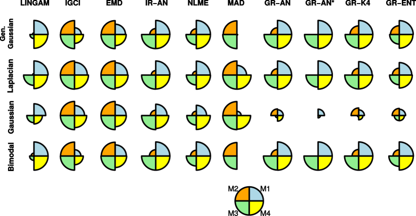
An overall comparison of the different methods evaluated is shown in Figure 6. This figure displays several radar charts that indicate the average accuracy of each method for the different types of noise considered and for each mechanism M1, M2, M3 and M4. In particular, for a given method and a given type of noise, the radius of each portion of the pie is proportional to the corresponding average accuracy of the method across the distributions $p_{1}$, $p_{2}$ and $p_{3}$ for the cause. The pie at the bottom corresponds to 100% accuracy for each causal mechanism. The conclusions derived from this figure are similar to the ones obtained from Table 1. In particular, IR-AN performs very well, except for multiplicative noise (M3), closely followed by GR-AN, $\text{GR-AN}^{\star}$, and GR-K4, which give similar results. The methods perform very poorly in the case of additive Gaussian noise, since they cannot infer the actual causal direction in that situation. NLME and GR-ENT have problems in the case of the causal mechanism M3 and MAD in the case of the mechanisms M1 and M4. LINGAM also performs bad in the case of M3 and IGCI and EMD have problems in the case of the mechanisms M1 and M4. IGCI, EMD and MAD are the only methods performing well in the case of M2, the mechanism with non-additive noise.

We have repeated these experiments for other samples sizes, e.g., 100, 200 300 and 1000. The results obtained are very similar to the ones reported here, except when the number of samples is small and equal to 100. In that case NLME performs slightly better than the proposed approach GR-AN, probably because with 100 samples it is very difficult to accurately estimate the non-linear transformation that is required to guarantee that $\mathcal{X}$ and $\mathcal{Y}$ are equally distributed. These results of these additional experiments are found in the supplementary material.

In summary, the good results provided by GR-AN and its variants in the experiments described indicate that (i) when the assumptions made by GR-AN are valid, the method has a good performance and (ii) there is indeed a Gaussianization effect in the residuals when the model is fitted under the anti-causal direction. Because $\text{GR-AN}^{\star}$ also performs well in these experiments, this indicates that a Gaussianization of the residuals may happen even when $\mathcal{X}$ and $\mathcal{Y}$ do not follow the same distribution.

Table 1: Accuracy on the synthetic data for each method, causal mechanisms and type of noise.

Noise	Generalized Gaussian				Laplacian				Gaussian				Bimodal
Algorithm	Mechanism				Mechanism				Mechanism				Mechanism
	M1	M2	M3	M4	M1	M2	M3	M4	M1	M2	M3	M4	M1	M2	M3	M4
$p_{1}(x)$
LINGAM	100%	1%	7%	93%	100%	0%	26%	89%	58%	0%	11%	12%	100%	0%	3%	100%
IGCI	28%	100%	100%	34%	73%	100%	100%	96%	49%	100%	100%	63%	29%	98%	100%	44%
EMD	34%	96%	100%	43%	70%	100%	100%	77%	48%	100%	100%	50%	50%	99%	100%	55%
IR-AN	100%	31%	100%	99%	99%	26%	100%	97%	45%	34%	100%	75%	100%	46%	100%	100%
NLME	100%	31%	22%	100%	100%	20%	15%	100%	45%	22%	8%	96%	100%	42%	17%	100%
MAD	0%	94%	100%	0%	100%	99%	100%	100%	50%	99%	100%	97%	0%	92%	97%	0%
GR-AN	100%	46%	95%	100%	100%	44%	80%	100%	48%	47%	6%	20%	100%	51%	100%	100%
$\text{GR-AN}^{\star}$	100%	0%	94%	100%	100%	0%	94%	100%	45%	0%	1%	17%	100%	0%	100%	100%
GR-K4	100%	70%	94%	100%	99%	51%	96%	100%	52%	56%	2%	19%	100%	53%	100%	100%
GR-ENT	100%	71%	76%	97%	93%	52%	51%	93%	41%	58%	26%	29%	100%	50%	84%	99%
$p_{2}(x)$
LINGAM	100%	32%	68%	100%	100%	30%	99%	100%	100%	13%	91%	100%	100%	53%	91%	100%
IGCI	40%	97%	100%	71%	98%	100%	100%	99%	72%	100%	100%	97%	39%	99%	100%	54%
EMD	96%	99%	100%	98%	96%	100%	100%	98%	94%	100%	100%	90%	92%	95%	100%	95%
IR-AN	100%	55%	100%	100%	100%	42%	100%	100%	100%	44%	100%	100%	100%	43%	100%	100%
NLME	100%	47%	100%	100%	95%	36%	100%	100%	99%	36%	100%	100%	100%	38%	100%	100%
MAD	0%	100%	100%	13%	5%	100%	100%	100%	2%	100%	100%	95%	0%	100%	85%	0%
GR-AN	100%	46%	100%	100%	98%	32%	96%	100%	29%	40%	16%	54%	100%	32%	100%	100%
$\text{GR-AN}^{\star}$	100%	0%	94%	100%	100%	0%	65%	100%	39%	0%	0%	6%	100%	0%	100%	100%
GR-K4	100%	50%	100%	100%	87%	44%	100%	98%	26%	51%	23%	47%	100%	30%	100%	100%
GR-ENT	96%	56%	90%	98%	78%	40%	73%	92%	46%	45%	42%	48%	100%	36%	97%	100%
$p_{3}(x)$
LINGAM	100%	0%	19%	100%	100%	0%	98%	100%	92%	0%	56%	67%	100%	8%	7%	100%
IGCI	76%	100%	100%	83%	100%	100%	100%	100%	92%	100%	100%	97%	67%	100%	100%	87%
EMD	90%	100%	100%	94%	98%	100%	100%	100%	92%	100%	100%	97%	96%	100%	100%	94%
IR-AN	100%	40%	100%	100%	100%	26%	100%	100%	96%	35%	100%	100%	100%	45%	100%	100%
NLME	100%	44%	100%	100%	100%	26%	100%	100%	74%	34%	98%	100%	100%	43%	99%	100%
MAD	0%	97%	100%	1%	100%	100%	100%	100%	38%	98%	100%	98%	0%	95%	99%	0%
GR-AN	100%	52%	90%	100%	100%	58%	100%	100%	46%	53%	36%	45%	100%	54%	98%	100%
$\text{GR-AN}^{\star}$	100%	0%	100%	100%	100%	0%	100%	100%	51%	0%	12%	26%	100%	0%	100%	100%
GR-K4	100%	64%	94%	100%	99%	47%	100%	97%	43%	54%	15%	24%	100%	57%	100%	100%
GR-ENT	100%	60%	42%	95%	94%	54%	86%	91%	47%	48%	48%	32%	100%	47%	43%	99%

Figure 6: Radar charts showing the average accuracy of each method for the different types of noise considered and for each mechanism M1, M2, M3 and M4. For a particular method and type of noise, the radius of each portion of the pie is proportional to the corresponding average accuracy of the method across the distributions $p_{1}$, $p_{2}$ and $p_{3}$ for the cause. The pie at the bottom corresponds to 100% accuracy for each mechanism.

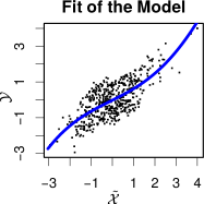
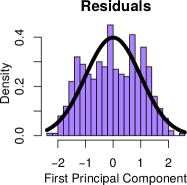
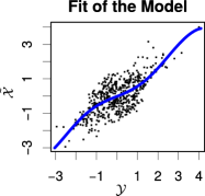
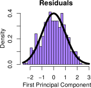
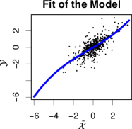
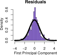
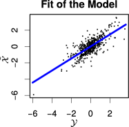
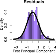
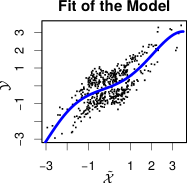
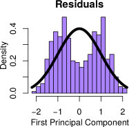
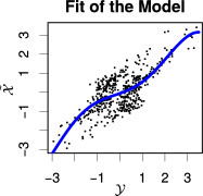
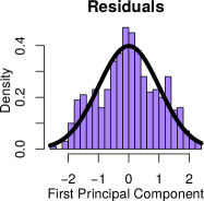
We give further evidence of the Gaussianization of the distribution of the residuals obtained when fitting the model under the anti-causal direction. For this, we analyze in detail three particular cases of GR-AN corresponding to the causal mechanism M3, the distribution $p_{2}(x)$ for the cause and each of the three types of additive noise considered. Namely, generalized Gaussian noise, Laplacian noise and bimodal noise. Figure 7 shows the predicted pre-images for new data instances when the model has been fitted in the causal ($\tilde{\mathcal{X}}\rightarrow\mathcal{Y}$) and the anti-causal ($\mathcal{Y}\rightarrow\tilde{\mathcal{X}}$) direction alongside with a histogram of the first principal component of the residuals in feature space. A Gaussian approximation is also displayed as a solid black line on top of the histogram. In this case $\mathbf{x}$, i.e., the samples of $\mathcal{X}$, have been transformed to be equally distributed to $\mathbf{y}$, i.e., the samples from $\mathcal{Y}$. We observe that the distribution of the residuals in the anti-causal direction ($\mathcal{Y}\rightarrow\tilde{\mathcal{X}}$) is more similar to a Gaussian distribution. Furthermore, for the direction $\tilde{\mathcal{X}}\rightarrow\mathcal{Y}$ the statistic of the energy based Gaussianity test for the first principal component of the residuals is respectively $4.02$, $4.64$ and $11.46$, for generalized Gaussian, Laplacian and bimodal noise. Recall that the larger the value the larger the deviation from Gaussianity. In the case of the direction $\mathcal{Y}\rightarrow\tilde{\mathcal{X}}$, the energy statistic associated to the residuals is $0.97$, $0.68$ and $1.31$, respectively. When $\mathbf{y}$ is transformed to have the same distribution as $\mathbf{x}$ similar results are observed (results not shown). However, the Gaussianization effect is not as strong as in this case, probably because it leads to the violation of the additive noise assumption. In summary, the figure displayed illustrates in detail the Gaussianization effect of the residuals when fitting the model in the anti-causal direction.

	Causal Direction ($\tilde{\mathcal{X}}\rightarrow\mathcal{Y})$		Anti-causal Direction ($\mathcal{Y}\rightarrow\tilde{\mathcal{X}})$
Gen. Gaussian
Laplacian
Bimodal

Figure 7: (left column) Predicted pre-images obtained in the casual direction $\tilde{\mathcal{X}}\rightarrow\mathcal{Y}$ alongside with a histogram of the first principal component of the residuals in feature space. A Gaussian fit is displayed as a solid black line. Results are shown for each type of additive noise considered. (right column) Same plots for the anti-causal direction $\mathcal{Y}\rightarrow\tilde{\mathcal{X}}$.

6.2 Experiments with real cause-effect pairs

A second batch of experiments is performed on the cause-effect pairs from the ChaLearn challenge. This challenge contains 8073 cause-effect data pairs with a labeled causal direction. From these pairs, we consider a subset for our experiments. In particular, we select the 184 pairs that have (i) at least $500$ samples, and (ii) a fraction of repeated instances for each random variable of at most $1\%$. The first criterion guarantees that there is enough data to make a decision with high confidence. The second criterion removes the pairs with discrete random variables, motivated by the transformation required by the GR-AN method to guarantee the equal distribution of $\mathcal{X}$ and $\mathcal{Y}$. In particular, this transformation cannot be carried out on discrete data. Another advantage is that this filtering process of the data facilitates the experiments since several of the methods considered in the comparison (i.e., GR-AN, GR-ENT, GR-K4, IR-AN, NLME, MAD and EMD) are computationally very expensive. More precisely, they have a cubic cost with respect to the number of samples and they require tuning several hyper-parameters. The consequence is that evaluating these methods on the 8073 pairs available is therefore not feasible.

Using these 184 pairs we evaluate each of the methods considered in the previous section and report the corresponding accuracy as a function of the decisions made. In these experiments we sample at random $500$ instances from each cause-effect pair. This is a standard number of samples that has been previously employed by other authors in their experiments with cause-effect pairs (Janzing et al., 2012). Furthermore, a threshold value is fixed and the obtained confidence in the decision by each method is compared to such threshold. Only if the confidence is above the threshold value, the cause-effect pair is considered in the evaluation of the accuracy of the corresponding method. A summary of the results is displayed in Figure 8. This figure shows for each method, as a fraction of the decisions made, the accuracy on the filtered datasets on which the confidence on the decision is above the threshold value. A gray area has been drawn to indicate accuracy values that are not statistically different from random guessing (accuracy equal to 50%) using a binomial test (p-value above 5%). We observe that IR-AN obtains the best results, followed by GR-AN, $\text{GR-AN}^{\star}$, GR-K4, GR-ENT, IGCI, NLME and EMD. NLME, IGCI and EMD perform worse than GR-AN and $\text{GR-AN}^{\star}$ when a high number of decisions are made. The differences in performance between IR-AN and GR-AN, when 100% of the decisions are made, are not statistically significant (a paired t-test returns a $p$-value equal to $25\%$). The fact that the performance of $\text{GR-AN}^{\star}$ is similar to the performance of GR-AN also indicates that there is some Gaussianization of the residuals even though the two random variables $\mathcal{X}$ and $\mathcal{Y}$ are not equally distributed. We observe that the results of LINGAM and MAD are not statistically different from random guessing. This remarks the importance of non-linear models and questions the practical utility of the MAD method. In these experiments, GR-ENT and GR-K4 perform worse than GR-AN, which remarks the benefits of using the energy distance to estimate the deviation from the Gaussian distribution, as a practical alternative to entropy or cumulant based measures.

In summary, the results displayed in Figure 8 confirm that the level of Gaussianity of the residuals, estimated using statistical tests, is a useful metric that can be used to identify the causal order of two random variables. Furthermore, this figure also validates the theoretical results obtained in Section 2 which state that one should expect residuals whose distribution is closer to the Gaussian distribution when performing a fit in the anti-causal direction.

In the supplementary material we include additional results for other sample sizes. Namely, $100$, $200$ and $300$ samples. The results obtained are similar to the ones reported in Figure 8. However, the differences between GR-ENT, NLME, GR-AN and $\text{GR-AN}^{\star}$ are smaller. Furthermore, when the number of samples is small (i.e., equal to $100$) GR-AN performs worse than NLME, probably because with such a small number of samples it is difficult to estimate the non-linear transformation that guarantees that $\mathcal{X}$ and $\mathcal{Y}$ are equality distributed.

Figure 8: Accuracy of each method, as a fraction of the decisions made, on the 184 filtered cause-effect pairs extracted from the ChaLearn challenge. The number of samples of each pair is equal to 500. Best seen in color.

Figure 9: Accuracy of each method, as a fraction of the decisions made, on the 82 cause-effect pairs extracted from the Tuebingen database. Best seen in color.

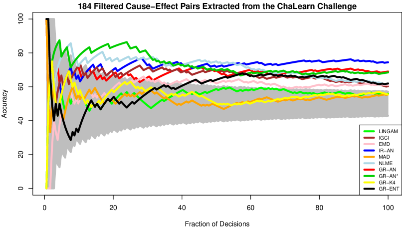
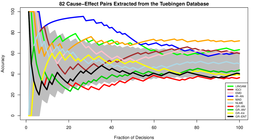
In this section we have also evaluated the different methods compared in the previous experiments on a random subset of 184 cause-effect pairs chosen across the 8073 pairs of the ChaLearn challenge (results not shown). In this case, the ranking of the curves obtained looks similar to the ranking displayed in Figure 8, i.e., IR-AN performs best followed by GR-AN, $\text{GR-AN}^{\star}$, NLME and EMD. However, all methods obtain worse results in general and none of them, except IR-AN, perform significantly different from random guessing.

Finally, we also have evaluated the different methods in a subset of 82 cause-effect pairs extracted from the Tübingen cause-effect pairs. We only considered those pairs with scalar cause and effect. The results obtained are displayed in Figure 9. In this case, the performance of the different methods is worse than the one displayed in Figure 8. Only IR-AN, IGCI and MAD perform significantly better than random guessing. Furthermore, GR-AN and $\text{GR-AN}^{\star}$ do not perform well in this set of cause-effect pairs. This is also the case of NLME. We believe that the reason for this bad performance is that in most of these pairs some of the variables take discrete or repeated values. In the case of GR-AN this makes infeasible to transform the two random variables, $\mathcal{X}$ and $\mathcal{Y}$, so that they are equally distributed. Furthermore, the discrete random variables may have a strong impact in the tests for Gaussianity and in the estimation of the differential entropy. This could explain the bad performance of $\text{GR-AN}^{\star}$, NLME and GR-ENT.

In summary, the results reported in this section have shown that in some cause-effect pairs, when the assumptions made by the proposed method are satisfied, there is indeed a Gaussianization effect in the residuals obtained when fitting the model in the anti-causal direction, and this asymmetry is useful to carry out causal inference on both synthetic and real inference problems. Our experiments also show that the transformation employed to guarantee that $\mathcal{X}$ and $\mathcal{Y}$ are equally distributed can be ignored in some cases without decreasing the performance. This indicates that our statement about the increased level of Gaussianity of the residuals, in terms of the increase of the entropy and the reduction of the high-order cumulants, may be true under more general assumptions.

7 Conclusions

In this paper we have shown that in the case of cause-effect pairs with additive non-Gaussian noise there is an asymmetry that can be used for causal inference. In particular, assuming that the cause and the effect are equally distributed random variables, that are linearly related, the residuals of a least squares fit in the anti-causal direction are more Gaussian than the residuals of a linear fit in the causal direction due a reduction of the magnitude of the high-order cumulants. Furthermore, by extending the results of Hyvärinen and Smith (2013) based on information theory, we have shown that this Gaussianization effect is also present when the two random variables are multivariate due to an increment of the differential entropy. This motivates the use of kernel methods to work in an expanded feature space. This enables addressing non-linear cause-effect inference problems using simple techniques. Specifically, kernel methods allow to fit a linear model in an expanded feature space which will be non-linear in the original input space.

Taking advantage of the asymmetry described, we have designed a method for non-linear causal inference, GR-AN (Gaussianity of the Residuals under Additive Noise). The method consists in computing the residuals of a linear model in an expanded feature space in both directions, i.e., $\mathcal{X}\rightarrow\mathcal{Y}$ and $\mathcal{Y}\rightarrow\mathcal{X}$. The expected causal direction is the one in which the residuals appear to be more Gaussian (i.e., the magnitude of the high-order cumulants is reduced and the entropy is increased). Thus, a suitable statistical test that measures the level of non-Gaussianity of the residuals can be used to determine the causal direction. In principle, one may be tempted to use statistical tests based on entropy or cumulant estimation. However, our experiments show that one can obtain better results by using a test based on an energy distance to quantify the Gaussianity of the residuals. In particular, entropy estimation is an arguably difficult task and the estimators of the cumulants involve high-order moments which can lead to high variance.

The effectiveness of the proposed method GR-AN has been illustrated in both synthetic and real-world causal inference problems. We have shown that in certain problems GR-AN is competitive with state-of-the-art methods and that it performs better than related methods based on entropy estimation (Hyvärinen and Smith, 2013). The entropy can be understood as a measure of non-Gaussianity. Nevertheless, it is very difficult to estimate in practice. By contrast, the statistical test employed by GR-AR is not directly related to entropy estimation. This may explain the improvements observed. A limitation of the current formulation of GR-AN is that the distributions of the cause and the effect have to be equal. In the case of continuous univariate variables finding a transformation to make this possible is straightforward. Additionally, our experiments show that such a transformation can be side-stepped in some cases without a deterioration in performance. In any case, further research is needed to extend this analysis to remove this restriction.

Finally, the performance of GR-AN on cause-effect pairs with discretized values is rather poor. We believe this is due to the fact that in this case, finding a transformation so that the cause and the effect are equally distributed is infeasible. Furthermore, the discretization process probably has a strong impact on the Gaussianity tests. Further evidence that make these observations more plausible is the fact that discretization has also a strong negative impact in the performance of the methods based on entropy estimation.

A

In this appendix we show that if $\mathcal{X}$ and $\mathcal{Y}$ follow the same distribution and they have been centered, then the determinant of the covariance matrix of the random variable corresponding to $\bm{\epsilon}_{i}$, denoted with $\text{Cov}(\bm{\epsilon}_{i})$, coincides with the determinant of the covariance matrix corresponding to the random variable $\tilde{\bm{\epsilon}}_{i}$, denoted with $\text{Cov}(\tilde{\bm{\epsilon}}_{i})$.

From the causal model, i.e., $\mathbf{y}_{i}=\mathbf{A}\mathbf{x}_{i}+\bm{\epsilon}_{i}$, we have that:

$$\text{Cov}(\mathcal{Y}) =\mathbf{A}\text{Cov}(\mathcal{X})\mathbf{A}^{\text{T}}+\text{Cov}(\bm{\epsilon}_{i})\,.$$ (48)

Since $\mathcal{X}$ and $\mathcal{Y}$ follow the same distribution we have that $\text{Cov}(\mathcal{Y})=\text{Cov}(\mathcal{X})$. Furthermore, we know from the causal model that $\mathbf{A}=\text{Cov}(\mathcal{Y},\mathcal{X})\text{Cov}(\mathcal{X})^{-1}$. Then,

$$\text{Cov}(\bm{\epsilon}_{i}) =\text{Cov}(\mathcal{X})-\text{Cov}(\mathcal{Y},\mathcal{X})\text{Cov}(\mathcal{X})^{-1}\text{Cov}(\mathcal{X},\mathcal{Y})\,.$$ (49)

In the case of $\tilde{\bm{\epsilon}}_{i}$ we know that the relation $\tilde{\bm{\epsilon}}_{i}=(\mathbf{I}-\tilde{\mathbf{A}}\mathbf{A})\mathbf{x}_{i}-\tilde{\mathbf{A}}\bm{\epsilon}_{i}$ must be satisfied, where $\tilde{\mathbf{A}}=\text{Cov}(\mathcal{X},\mathcal{Y})\text{Cov}(\mathcal{Y})^{-1}=\text{Cov}(\mathcal{X},\mathcal{Y})\text{Cov}(\mathcal{X})^{-1}$. Thus, we have that:

$$\text{Cov}(\tilde{\bm{\epsilon}}_{i}) =(\mathbf{I}-\tilde{\mathbf{A}}\mathbf{A})\text{Cov}(\mathcal{X})(\mathbf{I}-\mathbf{A}^{\text{T}}\tilde{\mathbf{A}}^{\text{T}})+\tilde{\mathbf{A}}\text{Cov}(\bm{\epsilon}_{i})\tilde{\mathbf{A}}^{\text{T}}$$

$$=\text{Cov}(\mathcal{X})-\text{Cov}(\mathcal{X})\mathbf{A}^{\text{T}}\tilde{\mathbf{A}}^{\text{T}}-\tilde{\mathbf{A}}\mathbf{A}\text{Cov}(\mathcal{X})+\tilde{\mathbf{A}}\mathbf{A}\text{Cov}(\mathcal{X})\mathbf{A}^{\text{T}}\tilde{\mathbf{A}}^{\text{T}}$$

$$\quad+\tilde{\mathbf{A}}\text{Cov}(\mathcal{X})\tilde{\mathbf{A}}^{\text{T}}-\tilde{\mathbf{A}}\text{Cov}(\mathcal{Y},\mathcal{X})\text{Cov}(\mathcal{X})^{-1}\text{Cov}(\mathcal{X},\mathcal{Y})\tilde{\mathbf{A}}^{\text{T}}$$

$$=\text{Cov}(\mathcal{X})-\text{Cov}(\mathcal{X})\mathbf{A}^{\text{T}}\tilde{\mathbf{A}}^{\text{T}}-\tilde{\mathbf{A}}\mathbf{A}\text{Cov}(\mathcal{X})+\tilde{\mathbf{A}}\text{Cov}(\mathcal{X})\tilde{\mathbf{A}}^{\text{T}}$$

$$=\text{Cov}(\mathcal{X})-\text{Cov}(\mathcal{X},\mathcal{Y})\text{Cov}{\mathcal{X}}^{-1}\text{Cov}(\mathcal{Y},\mathcal{X})-\text{Cov}(\mathcal{X},\mathcal{Y})\text{Cov}{\mathcal{X}}^{-1}\text{Cov}(\mathcal{Y},\mathcal{X})$$

$$\quad+\text{Cov}(\mathcal{X},\mathcal{Y})\text{Cov}{\mathcal{X}}^{-1}\text{Cov}(\mathcal{Y},\mathcal{X})$$

$$=\text{Cov}(\mathcal{X})-\text{Cov}(\mathcal{X},\mathcal{Y})\text{Cov}(\mathcal{X})^{-1}\text{Cov}(\mathcal{Y},\mathcal{X})\,.$$ (50)

By the matrix determinant theorem we have that $\text{det}\text{Cov}(\tilde{\bm{\epsilon}}_{i})=\text{det}\text{Cov}(\bm{\epsilon}_{i})$. See (Murphy, 2012, p. 117) for further details.

B

In this Appendix we motivate that, if the distribution of the residuals is not Gaussian, but is close to Gaussian, one should also expected more Gaussian residuals in the anti-causal direction in terms of the energy distance described in Section 3.4. For simplicity we will consider the univariate case. We use the fact that the energy distance in the one-dimensional case is the squared distance between the cumulative distribution functions of the residuals and a Gaussian distribution (Székely and Rizzo, 2013). Thus,

$$\tilde{D}^{2} =\int_{-\infty}^{\infty}\left[\tilde{F}(x)-\Phi(x)\right]^{2}dx\,, D^{2} =\int_{-\infty}^{\infty}\left[F(x)-\Phi(x)\right]^{2}dx\,,$$ (51)

where $\tilde{D}^{2}$ and $D^{2}$ are the energy distances to the Gaussian distribution in the anti-causal and the causal direction respectively; $\tilde{F}(x)$ and $F(x)$ are the c.d.f. of the residuals in the anti-causal and the causal direction, respectively; and finally, $\Phi(x)$ is the c.d.f. of a standard Gaussian.

One should expect that $\tilde{D}^{2}\leq D^{2}$. To motivate this, we use the Gram-Charlier series and compute an expansion of $\tilde{F}(x)$ and $F(x)$ around the standard Gaussian distribution (Patel and Read, 1996). Such an expansion only converges in the case of distributions that are close to be Gaussian (see Section 17.6.6a of (Cramér, 1946) for further details). Namely,

$$\tilde{F}(x) =\Phi(x)-\phi(x)\left(\frac{\tilde{a}_{3}}{3!}H_{2}(x)+\frac{\tilde{a}_{4}}{4!}H_{3}(x)+\cdots\right)\,,$$

$$F(x) =\Phi(x)-\phi(x)\left(\frac{a_{3}}{3!}H_{2}(x)+\frac{a_{4}}{4!}H_{3}(x)+\cdots\right)\,,$$ (52)

where $\phi(x)$ is the p.d.f. of a standard Gaussian, $H_{n}(x)$ are Hermite polynomials and $\tilde{a}_{n}$ and $a_{n}$ are coefficients that depend on the cumulants, e.g., $a_{3}=\kappa_{3}$, $a_{4}=\kappa_{4}$, $\tilde{a}_{3}=\tilde{\kappa}_{3}$, $\tilde{a}_{4}=\tilde{\kappa}_{4}$. Note, however, that coefficients $a_{n}$ and $\tilde{a}_{n}$ for $n>5$ depend on combinations of the cumulants. Using such an expansion we find:

$$\tilde{D}^{2} =\int_{-\infty}^{\infty}\phi(x)^{2}\left[-\sum_{n=3}^{\infty}\frac{\tilde{a}_{n}}{n!}H_{n-1}(x)\right]^{2}dx\approx\int_{-\infty}^{\infty}\phi(x)^{2}\left[-\sum_{n=3}^{4}\frac{\tilde{\kappa}_{n}}{n!}H_{n-1}(x)\right]^{2}dx$$

$$\approx\frac{\tilde{\kappa}_{3}^{2}}{36}\mathds{E}[H_{2}(x)^{2}\phi(x)]+\frac{\tilde{\kappa}_{4}^{2}}{576}\mathds{E}[H_{3}(x)^{2}\phi(x)]\,,$$ (53)

where $\mathds{E}[\cdot]$ denotes expectation with respect to a standard Gaussian and we have truncated the Gram-Charlier expansion after $n=4$. Truncation of the Gram-Charlier expansion after $n=4$ is a standard procedure that is often done in the ICA literature for entropy approximation. See for example Section 5.5.1 of (Hyvärinen et al., 2004). We have also used the fact that $\mathds{E}[H_{3}(x)H_{2}(x)\phi(x)]=0$. The same approach can be followed in the case of $D^{2}$, the energy distance in the causal direction. The consequence is that $D^{2}\approx\kappa_{3}^{2}/36\cdot\mathds{E}[H_{2}(x)^{2}\phi(x)]+\kappa_{4}^{2}/576\cdot\mathds{E}[H_{3}(x)^{2}\phi(x)]$. Finally, the fact that one should expect $\tilde{D}^{2}\leq D^{2}$ is obtained by noting that $\tilde{\kappa}_{n}=c_{n}\kappa_{n}$, where $c_{n}$ is some constant that lies in the interval $(-1,1)$, as indicated in Section 2.1. We expect that this result extends to the multivariate case.

C

In this Appendix we motivate that one should expect also more Gaussian residuals in the anti-causal direction, based on a reduction of the cumulants, when the residuals in feature space are projected onto the first principal component. That is, when they are multiplied by the first eigenvector of the covariance matrix of the residuals, and scaled by the corresponding eigenvalue. Recall from Section 2.2 that these covariance matrices are $\mathbf{C}=\mathbf{I}-\mathbf{A}\mathbf{A}^{\text{T}}$ and $\tilde{\mathbf{C}}=\mathbf{I}-\mathbf{A}^{\text{T}}\mathbf{A}$, in the causal and anti-causal direction respectively. Note that both matrices have the same eigenvalues.

If $\mathbf{A}$ is symmetric we have that both $\mathbf{C}$ and $\tilde{\mathbf{C}}$ have the same matrix of eigenvectors $\mathbf{P}$. Let $\mathbf{p}_{1}^{n}$ be the first eigenvector multiplied $n$ times using the Kronecker product. The cumulants in the anti-causal and the causal direction, after projecting the data onto the first eigenvector are $\tilde{\kappa}_{n}^{\text{proj}}=(\mathbf{p}_{1}^{\text{n}})^{\text{T}}\mathbf{M}_{n}\text{vect}(\tilde{\kappa}_{n})=c(\mathbf{p}_{1}^{\text{n}})^{\text{T}}\text{vect}(\tilde{\kappa}_{n})$ and $\kappa_{n}^{\text{proj}}=(\mathbf{p}_{1}^{\text{n}})^{\text{T}}\text{vect}(\kappa_{n})$, respectively, where $\mathbf{M}_{n}$ is the matrix that relates the cumulants in the causal and the anti-causal direction (see Section 2.2) and $c$ is one of the eigenvalues of $\mathbf{M}_{n}$. In particular, if $\mathbf{A}$ is symmetric, it is not difficult to show that $\mathbf{p}_{1}^{\text{n}}$ is one of the eigenvectors of $\mathbf{M}_{n}$. Furthermore, we also showed in that case that $||\mathbf{M}_{n}||_{\text{op}}<1$ for $n\geq 3$ (see Section 2.2). The consequence is that $c\in(-1,1)$, which combined with the fact that $||\mathbf{p}_{1}^{n}||=1$ leads to smaller cumulants in magnitude in the case of the projected residuals in the anti-causal direction.

If $\mathbf{A}$ is not symmetric we motivate that one should also expect more Gaussian residuals in the anti-causal direction due to a reduction in the magnitude of the cumulants. For this, we derive a smaller upper bound on their magnitude. This smaller upper bound is based on an argument that uses the operator norm of vectors.

Definition 2

The operator norm of a vector $\mathbf{w}$ induced by the $\ell_{p}$ norm is $||\mathbf{w}||_{\text{op}}=\text{min}\{c\geq 0:||\mathbf{w}^{\text{T}}\mathbf{v}||_{p}\leq c||\mathbf{v}||_{p},\forall\mathbf{v}\}$.

The consequence is that $||\mathbf{w}||_{\text{op}}\geq||\mathbf{w}^{\text{T}}\mathbf{v}||_{p}/||\mathbf{v}||_{p}$, $\forall\mathbf{v}$. Thus, the smallest the operator norm of $\mathbf{w}$, the smallest the expected value obtained when multiplying any vector by the vector $\mathbf{w}$. Furthermore, it is clear that $||\mathbf{w}||_{\text{op}}=||\mathbf{w}||_{2}$, in the case of the $\ell_{2}$-norm. From the previous paragraph, in the anti-causal direction we have $||\tilde{\kappa}_{n}^{\text{proj}}||_{2}=||(\tilde{\mathbf{p}}_{1}^{n})^{\text{T}}\mathbf{M}_{n}\text{vect}(\kappa_{n})||_{2}$, where $\tilde{\mathbf{p}}_{1}$ is the first eigenvector of $\tilde{\mathbf{C}}$, while in the causal direction we have $||\kappa_{n}^{\text{proj}}||_{2}=||(\mathbf{p}_{1}^{n})^{\text{T}}\text{vect}(\kappa_{n})||_{2}$, where $\mathbf{p}_{1}$ is the first eigenvector of $\mathbf{C}$. Thus, because the norm of each vector $\tilde{\mathbf{p}}_{1}^{n}$ and $\mathbf{p}_{1}^{n}$ is one, we have that $||\mathbf{p}_{1}^{n}||_{\text{op}}=1$. However, because we expect $\mathbf{M}_{n}$, to reduce the norm of $(\tilde{\mathbf{p}}_{1}^{n})^{\text{T}}$, as motivated in Section 2.2, $||(\tilde{\mathbf{p}}_{1}^{n})^{\text{T}}\mathbf{M}_{n}||_{\text{op}}<1$ should follow. This is expected to lead to smaller cumulants in magnitude in the anti-causal direction.

References

- Beirlant et al. (1997) J. Beirlant, E. J. Dudewicz, L. Györfi, and E. C. Van Der Meulen. Nonparametric entropy estimation: An overview. International Journal of Mathematical and Statistical Sciences, 6(1):17–39, 1997.
- Chen et al. (2013) Zhitang Chen, Kun Zhang, and Laiwan Chan. Nonlinear causal discovery for high dimensional data: A kernelized trace method. In IEEE 13th International Conference on Data Mining, pages 1003–1008, 2013.
- Chen et al. (2014) Zhitang Chen, Kun Zhang, Laiwan Chan, and Bernhard Schölkopf. Causal discovery via reproducing kernel Hilbert space embeddings. Neural Computation, 26(7):1484–1517, 2014.
- Cornish and Fisher (1938) E. A. Cornish and R. A. Fisher. Moments and cumulants in the specification of distributions. Revue de l’Institut International de Statistique / Review of the International Statistical Institute, 5(4):307–320, 1938.
- Cramér (1946) Harald Cramér. Mathematical methods of statistics. PhD thesis, 1946.
- Entner and Hoyer (2012) Doris Entner and PatrikO. Hoyer. Estimating a causal order among groups of variables in linear models. In Artificial Neural Networks and Machine Learning – ICANN 2012, pages 84–91. 2012.
- Gretton et al. (2008) Arthur Gretton, Kenji Fukumizu, Choon H. Teo, Le Song, Bernhard Schölkopf, and Alex J. Smola. A kernel statistical test of independence. In J.C. Platt, D. Koller, Y. Singer, and S.T. Roweis, editors, Advances in Neural Information Processing Systems 20, pages 585–592. 2008.
- Gretton et al. (2012) Arthur Gretton, Karsten M. Borgwardt, Malte J. Rasch, Bernhard Schölkopf, and Alexander Smola. A kernel two-sample test. Journal of Machine Learning Research, 13:723–773, 2012.
- Hernández-Lobato et al. (2011) José Miguel Hernández-Lobato, Pablo Morales-Mombiela, and Alberto Suárez. Gaussianity measures for detecting the direction of causal time series. In Proceedings of the 22nd International Joint Conference on Artificial Intelligence, pages 1318–1323, 2011.
- Hoyer et al. (2009) Patrik O. Hoyer, Dominik Janzing, Joris M. Mooij, Jonas Peters, and Bernhard Schölkopf. Nonlinear causal discovery with additive noise models. In D. Koller, D. Schuurmans, Y. Bengio, and L. Bottou, editors, Advances in Neural Information Processing Systems 21, pages 689–696, 2009.
- Hyvärinen (1998) Aapo Hyvärinen. New approximations of differential entropy for independent component analysis and projection pursuit. In Proceedings of the 1997 Conference on Advances in Neural Information Processing Systems 10, pages 273–279. MIT Press, 1998.
- Hyvärinen and Smith (2013) Aapo Hyvärinen and Stephen M. Smith. Pairwise likelihood ratios for estimation of non-gaussian structural equation models. Journal of Machine Learning Research, 14(1):111–152, 2013.
- Hyvärinen et al. (2004) Aapo Hyvärinen, Juha Karhunen, and Erkki Oja. Independent component analysis, volume 46. John Wiley & Sons, 2004.
- Janzing et al. (2010) Dominik Janzing, Patrik O. Hoyer, and Bernhard Schölkopf. Telling cause from effect based on high-dimensional observations. In Johannes Fürnkranz and Thorsten Joachims, editors, Proceedings of the 27th International Conference on Machine Learning (ICML-10), pages 479–486, 2010.
- Janzing et al. (2012) Dominik Janzing, Joris M. Mooij, Kun Zhang, Jan Lemeire, Jacob Zscheischler, Povilas Daniušis, Bastian Steudel, and Bernhard Schölkopf. Information-geometric approach to inferring causal directions. Artificial Intelligence, 182-183:1–31, 2012.
- Kawahara et al. (2012) Yoshinobu Kawahara, Kenneth Bollen, Shohei Shimizu, and Takashi Washio. GroupLiNGAM: Linear non-gaussian acyclic models for sets of variables. 2012. arXiv:1006.5041.
- Kpotufe et al. (2014) Samory Kpotufe, Eleni Sgouritsa, Dominik Janzing, and Bernhard Schölkopf. Consistency of causal inference under the additive noise model. In Proceedings of the 31th International Conference on Machine Learning, ICML 2014, Beijing, China, 21-26 June 2014, pages 478–486, 2014.
- Laub (2004) Alan J. Laub. Matrix Analysis For Scientists And Engineers. Society for Industrial and Applied Mathematics, Philadelphia, PA, USA, 2004. ISBN 0898715768.
- Marcinkiewicz (1938) J. T. Marcinkiewicz. Sur une propriété de la loi de gauss. Mathematische Zeitschrift, 44:612–618, 1938.
- McCullagh (1987) Peter McCullagh. Tensor methods in statistics. Chapman and Hall, 1987.
- Mooij et al. (2010) Joris M. Mooij, Oliver Stegle, Dominik Janzing, Kun Zhang, and Bernhard Schölkopf. Probabilistic latent variable models for distinguishing between cause and effect. In J.D. Lafferty, C.K.I. Williams, J. Shawe-Taylor, R.S. Zemel, and A. Culotta, editors, Advances in Neural Information Processing Systems 23, pages 1687–1695. 2010.
- Morales-Mombiela et al. (2013) Pablo Morales-Mombiela, Daniel Hernández-Lobato, and Alberto Suárez. Statistical tests for the detection of the arrow of time in vector autoregressive models. In Proceedings of the 23rd International Joint Conference on Artificial Intelligence, 2013.
- Murphy (2012) Kevin Murphy. Machine Learning: a Probabilistic Perspective. The MIT Press, 2012.
- Patel and Read (1996) Jagdish K Patel and Campbell B Read. Handbook of the normal distribution, volume 150. CRC Press, 1996.
- Pearl (2000) Judea Pearl. Causality: Models, Reasoning, and Inference. Cambridge University Press, New York, NY, USA, 2000. ISBN 0-521-77362-8.
- Schölkopf and Smola (2002) Bernhard Schölkopf and Alexander J. Smola. Learning with Kernels: Support Vector Machines, Regularization, Optimization, and Beyond. MIT Press, Cambridge, MA, USA, 2002. ISBN 0262194759.
- Schölkopf et al. (1997) Bernhard Schölkopf, Alexander Smola, and Klaus-Robert Müller. Kernel principal component analysis. In International Conference on Artificial Neural Networks, pages 583–588. Springer, 1997.
- Shimizu et al. (2006) Shohei Shimizu, Patrik O. Hoyer, Aapo Hyvärinen, and Antti Kerminen. A linear non-gaussian acyclic model for causal discovery. Journal of Machine Learning Research, 7:2003–2030, 2006.
- Singh et al. (2003) Harshinder Singh, Neeraj Misra, Vladimir Hnizdo, Adam Fedorowicz, and Eugene Demchuk. Nearest neighbor estimates of entropy. American journal of mathematical and management sciences, 23(3-4):301–321, 2003.
- Song et al. (2013) Le Song, K. Fukumizu, and A Gretton. Kernel embeddings of conditional distributions: A unified kernel framework for nonparametric inference in graphical models. Signal Processing Magazine, IEEE, 30:98–111, 2013.
- Székely and Rizzo (2005) Gábor J. Székely and Maria L. Rizzo. A new test for multivariate normality. Journal of Multivariate Analysis, 93(1):58–80, 2005.
- Székely and Rizzo (2013) Gábor J Székely and Maria L Rizzo. Energy statistics: A class of statistics based on distances. Journal of Statistical Planning and Inference, 143(8):1249–1272, 2013.
- Zhang and Hyvärinen (2009) Kun Zhang and Aapo Hyvärinen. On the identifiability of the post-nonlinear causal model. In Proceedings of the International Conference on Uncertainty in Artificial Intelligence, pages 647–655, 2009.