\addtokomafont

caption

FLAVOUR(267104)-ERC-80

𝑩𝑲()𝝂𝝂¯bold-→𝑩superscript𝑲𝝂bold-¯𝝂\bm{\mathsfit{B\to K^{(*)}\nu\bar{\nu}}} decays in the Standard Model and beyond

Andrzej J. Buras a,b, Jennifer Girrbach-Noe a,b, Christoph Niehoff c, and David M. Straub c
aTUM Institute for Advanced Study, Lichtenbergstr. 2a, 85748 Garching, Germany
bPhysik Department, TUM, James-Franck-Straße, 85748 Garching, Germany
cExcellence Cluster Universe, TUM, Boltzmannstr. 2, 85748 Garching, Germany

E-Mail: andrzej.buras@tum.de, jennifer.girrbach@tum.de, christoph.niehoff@tum.de, david.straub@tum.de

Abstract

We present an analysis of the rare exclusive B𝐵B decays BKνν¯𝐵𝐾𝜈¯𝜈B\to K\nu\bar{\nu} and BKνν¯𝐵superscript𝐾𝜈¯𝜈B\to K^{*}\nu\bar{\nu} within the Standard Model (SM), in a model-independent manner, and in a number of new physics (NP) models. Combining new form factor determinations from lattice QCD with light-cone sum rule results and including complete two-loop electroweak corrections to the SM Wilson coefficient, we obtain the SM predictions BR(B+K+νν¯)=(4.0±0.5)×106BRsuperscript𝐵superscript𝐾𝜈¯𝜈plus-or-minus4.00.5superscript106\text{BR}(B^{+}\to K^{+}\nu\bar{\nu})=(4.0\pm 0.5)\times 10^{-6} and BR(B0K0νν¯)=(9.2±1.0)×106BRsuperscript𝐵0superscript𝐾absent0𝜈¯𝜈plus-or-minus9.21.0superscript106\text{BR}(B^{0}\to K^{*0}\nu\bar{\nu})=(9.2\pm 1.0)\times 10^{-6}, more precise and more robust than previous estimates. Beyond the SM, we make use of an effective theory with dimension-six operators invariant under the SM gauge symmetries to relate NP effects in bsνν¯𝑏𝑠𝜈¯𝜈b\to s\nu\bar{\nu} transitions to bs+𝑏𝑠superscriptsuperscriptb\to s\ell^{+}\ell^{-} transitions and use the wealth of experimental data on BK()+𝐵superscript𝐾superscriptsuperscriptB\to K^{(*)}\ell^{+}\ell^{-} and related modes to constrain NP effects in BK()νν¯𝐵superscript𝐾𝜈¯𝜈B\to K^{(*)}\nu\bar{\nu}. We then consider several specific NP models, including Zsuperscript𝑍Z^{\prime} models, the MSSM, models with partial compositeness, and leptoquark models, demonstrating that the correlations between bsνν¯𝑏𝑠𝜈¯𝜈b\to s\nu\bar{\nu} observables among themselves and with Bsμ+μsubscript𝐵𝑠superscript𝜇superscript𝜇B_{s}\to\mu^{+}\mu^{-} and bs+𝑏𝑠superscriptsuperscriptb\to s\ell^{+}\ell^{-} transitions offer powerful tests of NP with new right-handed couplings and non-MFV interactions.

1 Introduction

Rare K𝐾K and B𝐵B decays with a neutrino pair in the final state, belonging to the theoretically cleanest in the field of flavour-changing neutral current (FCNC) processes, should soon play an important role in the tests of the Standard Model (SM) and its extensions111Recent reviews can be found in [1, 2]. This is due to a number of experiments being either planned or in preparation. Provided the rates of these decays are not significantly smaller than predicted within the SM, at the end of this decade we should have rather precise measurements of their branching ratios at our disposal.

As the search for new physics (NP) through these decays is based on possible deviations from SM predictions, it is crucial that the latter are as precise as possible. In the case of the decays K+π+νν¯superscript𝐾superscript𝜋𝜈¯𝜈K^{+}\rightarrow\pi^{+}\nu\bar{\nu} and KLπ0νν¯subscript𝐾𝐿superscript𝜋0𝜈¯𝜈K_{L}\rightarrow\pi^{0}\nu\bar{\nu}, the hadronic uncertainties are very small as the relevant hadronic matrix elements can be extracted from the leading semi-leptonic K+superscript𝐾K^{+} and KLsubscript𝐾𝐿K_{L} decays using isospin symmetry. For the decays BKνν¯𝐵superscript𝐾𝜈¯𝜈B\to K^{*}\nu\bar{\nu} and BKνν¯𝐵𝐾𝜈¯𝜈B\to K\nu\bar{\nu}, this is not possible, so studying them requires the evaluation of the relevant form factors by means of non-perturbative methods. The corresponding perturbative, short distance QCD and electroweak effects are also important but as we will summarize below they are by now fully under control. Most importantly, the decays based on the bsνν¯𝑏𝑠𝜈¯𝜈b\to s\nu\bar{\nu} transition do not suffer from hadronic uncertainties beyond the form factors, that plague the bs+𝑏𝑠superscriptsuperscriptb\to s\ell^{+}\ell^{-} transitions due to the breaking of factorization caused by photon exchange. For the BK()νν¯𝐵superscript𝐾𝜈¯𝜈B\to K^{(*)}\nu\bar{\nu} transitions, factorization is exact, so a measurement of the decay rates would allow in principle to measure the form factors. In the last two years, lattice computations of BK𝐵𝐾B\to K and BK𝐵superscript𝐾B\to K^{*} form factors have become available [3, 4] that are valid at large q2superscript𝑞2q^{2} of the neutrino pair and which complement the existing results within light-cone sum rules (LCSR) [5, 6, 7], valid at low and intermediate q2superscript𝑞2q^{2}. Combining these two sources of information, we will give SM predictions for the observables valid in the entire kinematic range, not relying on model-dependent extrapolations.

The relation between bsνν¯𝑏𝑠𝜈¯𝜈b\to s\nu\bar{\nu} and bs+𝑏𝑠superscriptsuperscriptb\to s\ell^{+}\ell^{-} processes is not just relevant in the SM, where they are governed by the same form factors, but also beyond the SM, since the SU(2)L𝑆𝑈subscript2𝐿SU(2)_{L} gauge symmetry relates neutrinos to left-handed charged leptons. The absence of any direct NP signal close to the electroweak scale at the LHC implies that this symmetry should still be reflected approximately in low-energy observables. This fact can be exploited by considering dimension-6 operators of SM fields invariant under the SM gauge symmetry222Such EFT approach has received increasing interest in the context of flavour physics recently, see e.g. [8, 9, 10]., some of which contribute to bsνν¯𝑏𝑠𝜈¯𝜈b\to s\nu\bar{\nu} and bs+𝑏𝑠superscriptsuperscriptb\to s\ell^{+}\ell^{-} processes simultaneously. This correlation is particularly interesting in view of various tensions with the SM recently observed in exclusive bs+𝑏𝑠superscriptsuperscriptb\to s\ell^{+}\ell^{-} decays [11, 12, 13, 14, 15, 16] that, if due to NP, might also leave an imprint in bsνν¯𝑏𝑠𝜈¯𝜈b\to s\nu\bar{\nu} decays. Although on a completely model-independent basis, no general conclusions can be drawn, it turns out that in specific NP models, often only a subset of these operators are present and we will demonstrate for several models that clear-cut predictions for the size of the effects and various correlations can be obtained.

In 2009, a detailed analysis of BKνν¯𝐵superscript𝐾𝜈¯𝜈B\to K^{*}\nu\bar{\nu}, BKνν¯𝐵𝐾𝜈¯𝜈B\to K\nu\bar{\nu} and BXsνν¯𝐵subscript𝑋𝑠𝜈¯𝜈B\to X_{s}\nu\bar{\nu} has been presented [17], giving the SM predictions and studying correlations among these decays as well as with sdνν¯𝑠𝑑𝜈¯𝜈s\to d\nu\bar{\nu} and bs+𝑏𝑠superscriptsuperscriptb\to s\ell^{+}\ell^{-} processes. Most importantly, it has been pointed out that these correlations offer powerful tests of NP with new right-handed couplings and non-MFV interactions. Several of the formulae presented in that paper have been used since then in the study of a number of NP models [18, 19, 20, 21, 22, 23, 24, 25]. For earlier studies of bsνν¯𝑏𝑠𝜈¯𝜈b\to s\nu\bar{\nu} transitions, see in particular [26, 27].

As the flavour precision era will certainly be one of the frontiers of particle physics in the second half of this decade, it is the right time to have a closer look at these decays with the goal to improve the accuracy of SM predictions and to generalize the NP study beyond the one presented in [17]. Here we summarize the main novelties in our present paper.

  • We update the SM predictions for the BK()νν¯𝐵superscript𝐾𝜈¯𝜈B\to K^{(*)}\nu\bar{\nu} branching ratios and the angular observable FLsubscript𝐹𝐿F_{L} in BKνν¯𝐵superscript𝐾𝜈¯𝜈B\to K^{*}\nu\bar{\nu}, using a combined fit of the BK𝐵𝐾B\to K and BK𝐵superscript𝐾B\to K^{*} form factors to LCSR and lattice calculations, making the SM predictions not only more precise, but also more reliable;

  • We include the complete two-loop electroweak corrections to the SM Wilson coefficient;

  • We discuss the model-independent implications of the precise measurements of BKμ+μ𝐵superscript𝐾superscript𝜇superscript𝜇B\to K^{*}\mu^{+}\mu^{-} and BKμ+μ𝐵𝐾superscript𝜇superscript𝜇B\to K\mu^{+}\mu^{-} observables at LHCb on BK()νν¯𝐵superscript𝐾𝜈¯𝜈B\to K^{(*)}\nu\bar{\nu}, using dimension-6 operators invariant under the SM gauge symmetry;

  • We investigate the impact of departing from lepton flavour universality;

  • We discuss predictions for BK()νν¯𝐵superscript𝐾𝜈¯𝜈B\to K^{(*)}\nu\bar{\nu} in several NP models, including Zsuperscript𝑍Z^{\prime} models, the MSSM, and models with scalar or vector leptoquarks;

  • We stress and demonstrate both in the model-independent approach and in the context of general Zsuperscript𝑍Z^{\prime} models that the correlations of the recently measured rate for Bsμ+μsubscript𝐵𝑠superscript𝜇superscript𝜇B_{s}\to\mu^{+}\mu^{-} with the rates for BK()νν¯𝐵superscript𝐾𝜈¯𝜈B\to K^{(*)}\nu\bar{\nu} and BK()μ+μ𝐵superscript𝐾superscript𝜇superscript𝜇B\to K^{(*)}\mu^{+}\mu^{-} offer particularly powerful tests of the presence of right-handed currents.

  • We point out that the decays BK()νν¯𝐵superscript𝐾𝜈¯𝜈B\to K^{(*)}\nu\bar{\nu} allow to distinguish between Z𝑍Z and Zsuperscript𝑍Z^{\prime} explanations of the present departures of the data from SM predictions for Bsμ+μsubscript𝐵𝑠superscript𝜇superscript𝜇B_{s}\to\mu^{+}\mu^{-}, BKμ+μ𝐵superscript𝐾superscript𝜇superscript𝜇B\to K^{*}\mu^{+}\mu^{-} and BKμ+μ𝐵𝐾superscript𝜇superscript𝜇B\to K\mu^{+}\mu^{-} that is rather hard on the basis of these three decays alone.

Our paper is organized as follows. In section 2 we define most important observables and present improved results for them within the SM. In section 3 we present a general discussion of NP in the framework of effective theories. In section 4 we will present the results in a number of concrete NP models stressing the importance of correlations between various observables that allow to distinguish between these models. We summarize the main results of our paper and conclude in section 5. The detailed information on form factors and various definitions are relegated to appendix A.

2 Standard Model

2.1 Effective Hamiltonian and observables

The effective Hamiltonian for bsνν¯𝑏𝑠𝜈¯𝜈b\to s\nu\bar{\nu} transitions in the SM reads

effSM=4GF2VtbVtsCLSM𝒪L+h.c.,superscriptsubscripteffSM4subscript𝐺𝐹2subscript𝑉𝑡𝑏superscriptsubscript𝑉𝑡𝑠superscriptsubscript𝐶𝐿SMsubscript𝒪𝐿h.c.{\mathcal{H}}_{\text{eff}}^{\text{SM}}=-\frac{4\,G_{F}}{\sqrt{2}}V_{tb}V_{ts}^{*}C_{L}^{\text{SM}}\mathcal{O}_{L}\leavevmode\nobreak\ +\leavevmode\nobreak\ \text{h.c.}\,, (1)

where

𝒪Lsubscript𝒪𝐿\displaystyle\mathcal{O}_{L} =e216π2(s¯γμPLb)(ν¯γμ(1γ5)ν).absentsuperscript𝑒216superscript𝜋2¯𝑠subscript𝛾𝜇subscript𝑃𝐿𝑏¯𝜈superscript𝛾𝜇1subscript𝛾5𝜈\displaystyle=\frac{e^{2}}{16\pi^{2}}(\bar{s}\gamma_{\mu}P_{L}b)(\bar{\nu}\gamma^{\mu}(1-\gamma_{5})\nu)\,. (2)

The Wilson coefficient CLSMsuperscriptsubscript𝐶𝐿SMC_{L}^{\text{SM}} is known with a high accuracy, including NLO QCD corrections [28, 29, 30] and two-loop electroweak contributions [31], resulting in

CLSMsuperscriptsubscript𝐶𝐿SM\displaystyle C_{L}^{\text{SM}} =Xt/sw2,absentsubscript𝑋𝑡superscriptsubscript𝑠𝑤2\displaystyle=-X_{t}/s_{w}^{2}\,, Xtsubscript𝑋𝑡\displaystyle X_{t} =1.469±0.017.absentplus-or-minus1.4690.017\displaystyle=1.469\pm 0.017\,. (3)

Since the neutrinos escape the detector unmeasured, there are three observables that can be measured in the decays BK()νν¯𝐵superscript𝐾𝜈¯𝜈B\to K^{(*)}\nu\bar{\nu} as functions of q2superscript𝑞2q^{2}: the two differential branching ratios and the Ksuperscript𝐾K^{*} longitudinal polarization fraction FLsubscript𝐹𝐿F_{L} in BKνν¯𝐵superscript𝐾𝜈¯𝜈B\to K^{*}\nu\bar{\nu}, first suggested in [17]. In the SM, they can be written as

dBR(B+K+νν¯)SMdq2𝑑BRsubscriptsuperscript𝐵superscript𝐾𝜈¯𝜈SM𝑑superscript𝑞2\displaystyle\frac{d\text{BR}(B^{+}\to K^{+}\nu\bar{\nu})_{\text{SM}}}{dq^{2}} KSM(q2)=τB+3|N|2Xt2sw4ρK(q2),absentsuperscriptsubscript𝐾SMsuperscript𝑞2subscript𝜏superscript𝐵3superscript𝑁2superscriptsubscript𝑋𝑡2superscriptsubscript𝑠𝑤4subscript𝜌𝐾superscript𝑞2\displaystyle\equiv\mathcal{B}_{K}^{\text{SM}}(q^{2})=\tau_{B^{+}}3|N|^{2}\frac{X_{t}^{2}}{s_{w}^{4}}\rho_{K}(q^{2}), (4)
dBR(B0K0νν¯)SMdq2𝑑BRsubscriptsuperscript𝐵0superscript𝐾absent0𝜈¯𝜈SM𝑑superscript𝑞2\displaystyle\frac{d\text{BR}(B^{0}\to K^{*0}\nu\bar{\nu})_{\text{SM}}}{dq^{2}} KSM(q2)=τB03|N|2Xt2sw4[ρA1(q2)+ρA12(q2)+ρV(q2)],absentsuperscriptsubscriptsuperscript𝐾SMsuperscript𝑞2subscript𝜏superscript𝐵03superscript𝑁2superscriptsubscript𝑋𝑡2superscriptsubscript𝑠𝑤4delimited-[]subscript𝜌subscript𝐴1superscript𝑞2subscript𝜌subscript𝐴12superscript𝑞2subscript𝜌𝑉superscript𝑞2\displaystyle\equiv\mathcal{B}_{K^{*}}^{\text{SM}}(q^{2})=\tau_{B^{0}}3|N|^{2}\frac{X_{t}^{2}}{s_{w}^{4}}\left[\rho_{A_{1}}(q^{2})+\rho_{A_{12}}(q^{2})+\rho_{V}(q^{2})\right], (5)
FL(BKνν¯)SMsubscript𝐹𝐿subscript𝐵superscript𝐾𝜈¯𝜈SM\displaystyle F_{L}(B\to K^{*}\nu\bar{\nu})_{\text{SM}} FLSM(q2)=ρA12(q2)ρA1(q2)+ρA12(q2)+ρV(q2),absentsuperscriptsubscript𝐹𝐿SMsuperscript𝑞2subscript𝜌subscript𝐴12superscript𝑞2subscript𝜌subscript𝐴1superscript𝑞2subscript𝜌subscript𝐴12superscript𝑞2subscript𝜌𝑉superscript𝑞2\displaystyle\equiv F_{L}^{\text{SM}}(q^{2})=\frac{\rho_{A_{12}}(q^{2})}{\rho_{A_{1}}(q^{2})+\rho_{A_{12}}(q^{2})+\rho_{V}(q^{2})}, (6)

where the factor of 3 stems from the sum over neutrino flavours,

N=VtbVtsGFα16π2mB3π,𝑁subscript𝑉𝑡𝑏superscriptsubscript𝑉𝑡𝑠subscript𝐺𝐹𝛼16superscript𝜋2subscript𝑚𝐵3𝜋N=V_{tb}V_{ts}^{*}\,\frac{G_{F}\alpha}{16\pi^{2}}\sqrt{\frac{m_{B}}{3\pi}}\,, (7)

is a normalization factor and the ρisubscript𝜌𝑖\rho_{i} are rescaled form factors defined in appendix A. In contrast to BK()+𝐵superscript𝐾superscriptsuperscriptB\to K^{(*)}\ell^{+}\ell^{-} decays, the isospin asymmetries of the decays with neutrinos in the final state vanish identically, so the branching ratio of the B0superscript𝐵0B^{0} and B±superscript𝐵plus-or-minusB^{\pm} decays only differ due to the lifetime difference. FLsubscript𝐹𝐿F_{L} is equal for charged and neutral B𝐵B decay.

We also define q2superscript𝑞2q^{2}-binned observables

K()SM[a,b]subscriptdelimited-⟨⟩superscriptsubscriptsuperscript𝐾SM𝑎𝑏\displaystyle\left\langle\mathcal{B}_{K^{(*)}}^{\text{SM}}\right\rangle_{[a,b]} ab𝑑q2dBR(BK()νν¯)SMdq2,absentsuperscriptsubscript𝑎𝑏differential-dsuperscript𝑞2𝑑BRsubscript𝐵superscript𝐾𝜈¯𝜈SM𝑑superscript𝑞2\displaystyle\equiv\int_{a}^{b}dq^{2}\leavevmode\nobreak\ \frac{d\text{BR}(B\to K^{(*)}\nu\bar{\nu})_{\text{SM}}}{dq^{2}}\,, (8)
FLSM[a,b]subscriptdelimited-⟨⟩superscriptsubscript𝐹𝐿SM𝑎𝑏\displaystyle\left\langle F_{L}^{\text{SM}}\right\rangle_{[a,b]} ab𝑑q2ρA12(q2)ab𝑑q2[ρA1(q2)+ρA12(q2)+ρV(q2)].absentsuperscriptsubscript𝑎𝑏differential-dsuperscript𝑞2subscript𝜌subscript𝐴12superscript𝑞2superscriptsubscript𝑎𝑏differential-dsuperscript𝑞2delimited-[]subscript𝜌subscript𝐴1superscript𝑞2subscript𝜌subscript𝐴12superscript𝑞2subscript𝜌𝑉superscript𝑞2\displaystyle\equiv\frac{\int_{a}^{b}dq^{2}\rho_{A_{12}}(q^{2})}{\int_{a}^{b}dq^{2}\left[\rho_{A_{1}}(q^{2})+\rho_{A_{12}}(q^{2})+\rho_{V}(q^{2})\right]}\,. (9)

2.2 Numerical analysis

The numerical prediction of the observables within the SM requires the calculation of the hadronic form factors. Both for BK𝐵𝐾B\to K and BK𝐵superscript𝐾B\to K^{*}, lattice computations have become available recently [3, 4], that are valid at large q2superscript𝑞2q^{2}. At low q2superscript𝑞2q^{2}, we make use of the results from light-cone sum rules [5, 6]. Since the form factors have to be smooth functions of q2superscript𝑞2q^{2}, one can obtain expressions valid in the whole kinematical range relevant for BK()νν¯𝐵superscript𝐾𝜈¯𝜈B\to K^{(*)}\nu\bar{\nu} by performing a combined fit to lattice and LCSR results. Since this approach makes use of theoretical input on both ends of the kinematical range, the results will be very weakly dependent on the parametrization chosen for the form factors. In the case of BK𝐵superscript𝐾B\to K^{*}, such combined fit has been performed recently in [32]. For BK𝐵𝐾B\to K, we have performed our own fit that we discuss in detail in appendix A.

sw2superscriptsubscript𝑠𝑤2s_{w}^{2} 0.23126(5)0.2312650.23126(5) [33, 31] τB0subscript𝜏superscript𝐵0\tau_{B^{0}} 1.519(5)1.51951.519(5) ps [33]
α𝛼\alpha 127.925(16)127.92516127.925(16) [33, 31] τB+subscript𝜏superscript𝐵\tau_{B^{+}} 1.638(4)1.63841.638(4) ps [33]
|VtbVts|subscript𝑉𝑡𝑏superscriptsubscript𝑉𝑡𝑠|V_{tb}V_{ts}^{*}| 0.0401(10)0.0401100.0401(10) [34, 35] mb1Ssuperscriptsubscript𝑚𝑏1Sm_{b}^{\text{1S}} 4.66(3)4.6634.66(3) GeV [33]
Table 1: Input parameters used for the SM predictions.

Our numerical results for the differential branching ratios and FLsubscript𝐹𝐿F_{L} are given in table 2 for different bins of q2superscript𝑞2q^{2} and for the whole kinematical region. The total branching ratios in the SM are shown in the last row, as the results of integrating over the whole kinematically allowed region,

BR(B+K+νν¯)SMBRsubscriptsuperscript𝐵superscript𝐾𝜈¯𝜈SM\displaystyle\text{BR}(B^{+}\to K^{+}\nu\bar{\nu})_{\text{SM}} =(3.98±0.43±0.19)×106,absentplus-or-minus3.980.430.19superscript106\displaystyle=(3.98\pm 0.43\pm 0.19)\times 10^{-6}, (10)
BR(B0K0νν¯)SMBRsubscriptsuperscript𝐵0superscript𝐾absent0𝜈¯𝜈SM\displaystyle\text{BR}(B^{0}\to K^{*0}\nu\bar{\nu})_{\text{SM}} =(9.19±0.86±0.50)×106,absentplus-or-minus9.190.860.50superscript106\displaystyle=(9.19\pm 0.86\pm 0.50)\times 10^{-6}, (11)
FLSMsubscriptsuperscript𝐹SM𝐿\displaystyle F^{\text{SM}}_{L} =0.47±0.03,absentplus-or-minus0.470.03\displaystyle=0.47\pm 0.03\,, (12)

where the first error is due to the form factors and the second one parametric. From table 1, summarizing the numerical input used for these predictions, one can see that the parametric error is completely dominated by CKM elements. We note that, when determined from tree-level decays, the uncertainty on the CKM combination |VtbVts|subscript𝑉𝑡𝑏superscriptsubscript𝑉𝑡𝑠|V_{tb}V_{ts}^{*}| is dominated by the uncertainty on |Vcb|subscript𝑉𝑐𝑏|V_{cb}| and our value corresponds to |Vcb|=0.0409(10)subscript𝑉𝑐𝑏0.040910|V_{cb}|=0.0409(10). Using instead the PDG averages of the inclusive or exlusive determinations, respectively, which are at a 2.5σ2.5𝜎2.5\sigma tension with each other [33], the central values of the branching ratios would shift by 7% up or down, respectively [16].

As seen from (6), in FLsubscript𝐹𝐿F_{L} all these parametric uncertainties cancel, so we only quote the form factor uncertainty. Note that the value of FLsubscript𝐹𝐿F_{L} at the kinematical endpoints is fixed [17, 36].

q2superscript𝑞2q^{2} [GeV]2 106KSMsuperscript106delimited-⟨⟩superscriptsubscriptsuperscript𝐾SM10^{6}\left\langle\mathcal{B}_{K^{*}}^{\text{SM}}\right\rangle κηsubscript𝜅𝜂\kappa_{\eta} FLSMdelimited-⟨⟩superscriptsubscript𝐹𝐿SM\left\langle F_{L}^{\text{SM}}\right\rangle 106KSMsuperscript106delimited-⟨⟩superscriptsubscript𝐾SM10^{6}\left\langle\mathcal{B}_{K}^{\text{SM}}\right\rangle
04040-4 1.38±0.21±0.07plus-or-minus1.380.210.071.38\pm 0.21\pm 0.07 1.64±0.04plus-or-minus1.640.041.64\pm 0.04 0.79±0.03plus-or-minus0.790.030.79\pm 0.03 0.93±0.14±0.05plus-or-minus0.930.140.050.93\pm 0.14\pm 0.05
48484-8 1.88±0.22±0.10plus-or-minus1.880.220.101.88\pm 0.22\pm 0.10 1.28±0.05plus-or-minus1.280.051.28\pm 0.05 0.56±0.03plus-or-minus0.560.030.56\pm 0.03 0.92±0.11±0.04plus-or-minus0.920.110.040.92\pm 0.11\pm 0.04
8128128-12 2.27±0.22±0.12plus-or-minus2.270.220.122.27\pm 0.22\pm 0.12 1.16±0.05plus-or-minus1.160.051.16\pm 0.05 0.43±0.03plus-or-minus0.430.030.43\pm 0.03 0.86±0.09±0.04plus-or-minus0.860.090.040.86\pm 0.09\pm 0.04
1216121612-16 2.36±0.18±0.13plus-or-minus2.360.180.132.36\pm 0.18\pm 0.13 1.24±0.05plus-or-minus1.240.051.24\pm 0.05 0.35±0.02plus-or-minus0.350.020.35\pm 0.02 0.71±0.07±0.03plus-or-minus0.710.070.030.71\pm 0.07\pm 0.03
16qmax216subscriptsuperscript𝑞2max16-q^{2}_{\text{max}} 1.30±0.10±0.07plus-or-minus1.300.100.071.30\pm 0.10\pm 0.07 1.57±0.05plus-or-minus1.570.051.57\pm 0.05 0.32±0.03plus-or-minus0.320.030.32\pm 0.03 0.55±0.05±0.04plus-or-minus0.550.050.040.55\pm 0.05\pm 0.04
0qmax20subscriptsuperscript𝑞2max0-q^{2}_{\text{max}} 9.19±0.86±0.50plus-or-minus9.190.860.509.19\pm 0.86\pm 0.50 1.34±0.04plus-or-minus1.340.041.34\pm 0.04 0.47±0.03plus-or-minus0.470.030.47\pm 0.03 3.98±0.43±0.19plus-or-minus3.980.430.193.98\pm 0.43\pm 0.19
Table 2: Results for various quantities as defined in the text. qmax2subscriptsuperscript𝑞2maxq^{2}_{\text{max}} is the kinematic limit of 22.9 GeV in the case of BKνν¯𝐵𝐾𝜈¯𝜈B\to K\nu\bar{\nu} and 19.2 GeV for BKνν¯𝐵superscript𝐾𝜈¯𝜈B\to K^{*}\nu\bar{\nu}. For the differential branching ratios, the first error is due to the form factors and the second one due to parametric uncertainties (including the parameters in table 1 as well as Xtsubscript𝑋𝑡X_{t}). For the other quantities, parametric uncertainties are negligible.

Our result for the B+K+νν¯superscript𝐵superscript𝐾𝜈¯𝜈B^{+}\to K^{+}\nu\bar{\nu} branching ratio is compatible with – but significantly more precise than – earlier determinations [17, 37]. In the case of the BKνν¯𝐵superscript𝐾𝜈¯𝜈B\to K^{*}\nu\bar{\nu} branching ratio, our new prediction is roughly 35% higher than the one of [17]. There are two main sources for this difference. First, we use the electromagnetic fine structure constant αemsubscript𝛼em\alpha_{\text{em}} in the MS¯¯MS\overline{\text{MS}} scheme at the scale MZsubscript𝑀𝑍M_{Z} rather than at zero momentum transfer. This is the correct choice to be used with the Wilson coefficient including NLO electroweak corrections in (3). In 2009, these corrections were not known yet, so the scheme and scale choice of αemsubscript𝛼em\alpha_{\text{em}} was a higher order effect. Second, the normalization of our form factors is fixed by the predictions of LCSR combined with the lattice predictions (which are in very good agreement). In [17], the LCSR prediction for the form factors was only used for the form factor shape and the relative normalization, while the overall normalization was extracted from the experimental measurement of BR(BKγ)BR𝐵superscript𝐾𝛾\text{BR}(B\to K^{*}\gamma), following [38, 39]. We do not follow this approach because it assumes the absence of NP in BKγ𝐵superscript𝐾𝛾B\to K^{*}\gamma. We also note that up-to-date experimental and theoretical predictions for BKγ𝐵superscript𝐾𝛾B\to K^{*}\gamma are in good agreement [32]. Finally, we note that the error estimates of [17] did not include the uncertainty due to the model dependence of the extrapolation of the LCSR form factors to high q2superscript𝑞2q^{2}. Our new predictions include this uncertainty (which is much reduced by the addition of the lattice data) and so they are not only more precise, but are also put on a more firm footing.

Our predictions should be compared with the present experimental upper bounds. Combining two analyses with hadronic or semi-leptonic tagging as well as charged and neutral B𝐵B decays, the BaBar collaboration finds [40]

BR(B+K+νν¯)BRsuperscript𝐵superscript𝐾𝜈¯𝜈\displaystyle\text{BR}(B^{+}\to K^{+}\nu\bar{\nu}) <1.7×10⁵(90%  CL).absent1.7superscript105(90%  CL)\displaystyle<1.7\times 10^{-5}\ \text{(90\%\, CL)}. (13)

The strongest bound on the BKνν¯𝐵superscript𝐾𝜈¯𝜈B\to K^{*}\nu\bar{\nu} decay was set by the Belle collaboration, [41]

BR(B0K0νν¯)BRsuperscript𝐵0superscript𝐾absent0𝜈¯𝜈\displaystyle\text{BR}(B^{0}\to K^{*0}\nu\bar{\nu}) <5.5×10⁵(90%  CL),absent5.5superscript105(90%  CL)\displaystyle<5.5\times 10^{-5}\ \text{(90\%\, CL)}, (14)
BR(B+K+νν¯)BRsuperscript𝐵superscript𝐾absent𝜈¯𝜈\displaystyle\text{BR}(B^{+}\to K^{*+}\nu\bar{\nu}) <4.0×10⁵(90%  CL).absent4.0superscript105(90%  CL)\displaystyle<4.0\times 10^{-5}\ \text{(90\%\, CL)}. (15)

Since BR(B+K()+νν¯)/BR(B0K()0νν¯)=τB+/τB0BRsuperscript𝐵superscript𝐾limit-from𝜈¯𝜈BRsuperscript𝐵0superscript𝐾0𝜈¯𝜈subscript𝜏superscript𝐵subscript𝜏superscript𝐵0\text{BR}(B^{+}\to K^{(*)+}\nu\bar{\nu})/\text{BR}(B^{0}\to K^{(*)0}\nu\bar{\nu})=\tau_{B^{+}}/\tau_{B^{0}} holds in the SM and beyond, we can use the stronger of these bounds and obtain

KKKSMsubscript𝐾subscript𝐾superscriptsubscript𝐾SM\displaystyle\mathcal{R}_{K}\equiv\frac{\mathcal{B}_{K}}{\mathcal{B}_{K}^{\text{SM}}} <4.3,absent4.3\displaystyle<4.3\,, KKKSMsubscriptsuperscript𝐾subscriptsuperscript𝐾superscriptsubscriptsuperscript𝐾SM\displaystyle\mathcal{R}_{K^{*}}\equiv\frac{\mathcal{B}_{K^{*}}}{\mathcal{B}_{K^{*}}^{\text{SM}}} <4.4,absent4.4\displaystyle<4.4\,, (16)

at 90% C.L., where we have neglected the theory uncertainty.

At the Belle-II experiment, a conservative estimate of the sensitivity with 50 ab-1, that is expected to be collected by 2023, envisages a measurement of the SM branching ratios with 30% precision [42] based on the predictions of [17]. Since we predict a significantly higher branching ratio for BKνν¯𝐵superscript𝐾𝜈¯𝜈B\to K^{*}\nu\bar{\nu} as discussed above, a better relative precision could be reached in turn. Moreover, already with 20 ab-1, that is expected to be collected by 2020, first signs of NP could in principle be seen. Indeed, we will see in sections 3 and 4 that in several NP models, the experimental upper bounds can be saturated. In this case, a 5σ5𝜎5\sigma discovery should be definitely possible at Belle-II.

3 Model-independent new physics analysis

3.1 Low-energy effective theory

Beyond the SM (but assuming no NP lighter than the B𝐵B meson), a second operator can appear in the effective low-energy Hamiltonian for bsνν¯𝑏𝑠𝜈¯𝜈b\to s\nu\bar{\nu} transitions,

eff=4GF2VtbVts(CL𝒪L+CR𝒪R)+h.c.,subscripteff4subscript𝐺𝐹2subscript𝑉𝑡𝑏superscriptsubscript𝑉𝑡𝑠subscript𝐶𝐿subscript𝒪𝐿subscript𝐶𝑅subscript𝒪𝑅h.c.{\mathcal{H}}_{\text{eff}}=-\frac{4\,G_{F}}{\sqrt{2}}V_{tb}V_{ts}^{*}\left(C_{L}\mathcal{O}_{L}+C_{R}\mathcal{O}_{R}\right)\leavevmode\nobreak\ +\leavevmode\nobreak\ \text{h.c.}\,, (17)

where

𝒪Lsubscript𝒪𝐿\displaystyle\mathcal{O}_{L} =e216π2(s¯γμPLb)(ν¯γμ(1γ5)ν),absentsuperscript𝑒216superscript𝜋2¯𝑠subscript𝛾𝜇subscript𝑃𝐿𝑏¯𝜈superscript𝛾𝜇1subscript𝛾5𝜈\displaystyle=\frac{e^{2}}{16\pi^{2}}(\bar{s}\gamma_{\mu}P_{L}b)(\bar{\nu}\gamma^{\mu}(1-\gamma_{5})\nu)\,, 𝒪Rsubscript𝒪𝑅\displaystyle\mathcal{O}_{R} =e216π2(s¯γμPRb)(ν¯γμ(1γ5)ν).absentsuperscript𝑒216superscript𝜋2¯𝑠subscript𝛾𝜇subscript𝑃𝑅𝑏¯𝜈superscript𝛾𝜇1subscript𝛾5𝜈\displaystyle=\frac{e^{2}}{16\pi^{2}}(\bar{s}\gamma_{\mu}P_{R}b)(\bar{\nu}\gamma^{\mu}(1-\gamma_{5})\nu)\,. (18)

In writing this effective Hamiltonian, we have explicitly assumed lepton flavour universality (LFU), i.e. that NP couples to all three neutrino flavours in the same manner. The implications of relaxing this assumption will be discussed in general terms at the end of this section and in section 4 in the context of leptoquark models.

In spite of the presence of two complex Wilson coefficients, the modification of the three observables can be described in terms of two real quantities ϵ>0italic-ϵ0\epsilon>0 and η[12,12]𝜂1212\eta\in[-\frac{1}{2},\frac{1}{2}], defined as

ϵ=|CL|2+|CR|2|CLSM|,η=Re(CLCR)|CL|2+|CR|2,formulae-sequenceitalic-ϵsuperscriptsubscript𝐶𝐿2superscriptsubscript𝐶𝑅2superscriptsubscript𝐶𝐿SM𝜂Resubscript𝐶𝐿superscriptsubscript𝐶𝑅superscriptsubscript𝐶𝐿2superscriptsubscript𝐶𝑅2\epsilon=\frac{\sqrt{|C_{L}|^{2}+|C_{R}|^{2}}}{|C_{L}^{\text{SM}}|}\leavevmode\nobreak\ ,\qquad\eta=\frac{-\text{Re}\left(C_{L}C_{R}^{*}\right)}{|C_{L}|^{2}+|C_{R}|^{2}}\leavevmode\nobreak\ , (19)

such that ϵ=1italic-ϵ1\epsilon=1 in the SM and η0𝜂0\eta\neq 0 signals the presence of right-handed currents. One finds

Ksubscript𝐾\displaystyle\mathcal{R}_{K} =(12η)ϵ2,absent12𝜂superscriptitalic-ϵ2\displaystyle=(1-2\,\eta)\epsilon^{2}\,, Ksubscriptsuperscript𝐾\displaystyle\mathcal{R}_{K^{*}} =(1+κηη)ϵ2,absent1subscript𝜅𝜂𝜂superscriptitalic-ϵ2\displaystyle=(1+\kappa_{\eta}\eta)\epsilon^{2}\,, FLFLFLSMsubscriptsubscript𝐹𝐿subscript𝐹𝐿superscriptsubscript𝐹𝐿SM\displaystyle\mathcal{R}_{F_{L}}\equiv\frac{F_{L}}{F_{L}^{\text{SM}}} =1+2η1+κηη.absent12𝜂1subscript𝜅𝜂𝜂\displaystyle=\frac{1+2\eta}{1+\kappa_{\eta}\eta}\,. (20)

The parameter κηsubscript𝜅𝜂\kappa_{\eta} depends on the form factors and its explicit form is given in appendix A. Its numerical value is listed in the last row of table 2.

Since the three observables in (20) only depend on two combinations of Wilson coefficients, there is a model-independent prediction,

FL=FLSM((κη2)K+4K(κη+2)K).subscript𝐹𝐿superscriptsubscript𝐹𝐿SMsubscript𝜅𝜂2subscript𝐾4subscriptsuperscript𝐾subscript𝜅𝜂2subscriptsuperscript𝐾F_{L}=F_{L}^{\text{SM}}\left(\frac{(\kappa_{\eta}-2)\mathcal{R}_{K}+4\,\mathcal{R}_{K^{*}}}{(\kappa_{\eta}+2)\mathcal{R}_{K^{*}}}\right)\,. (21)

In principle, this relation can be tested experimentally (also on a bin-by-bin basis). A similar relation can be obtained for the modification of the inclusive BXsνν¯𝐵subscript𝑋𝑠𝜈¯𝜈B\to X_{s}\nu\bar{\nu} branching ratio,

BR(BXsνν¯)BR(BXsνν¯)SM(κηK+2Kκη+2),BR𝐵subscript𝑋𝑠𝜈¯𝜈BRsubscript𝐵subscript𝑋𝑠𝜈¯𝜈SMsubscript𝜅𝜂subscript𝐾2subscriptsuperscript𝐾subscript𝜅𝜂2\text{BR}(B\to X_{s}\nu\bar{\nu})\approx\text{BR}(B\to X_{s}\nu\bar{\nu})_{\text{SM}}\left(\frac{\kappa_{\eta}\mathcal{R}_{K}+2\,\mathcal{R}_{K^{*}}}{\kappa_{\eta}+2}\right)\,, (22)

where we have neglected a contribution proportional to η𝜂\eta of at most ±5%plus-or-minuspercent5\pm 5\% to the inclusive branching ratio [17]. Following [17] and using our updated numerical input, we obtain

BR(BXsνν¯)SM=(2.9±0.3)×105.BRsubscript𝐵subscript𝑋𝑠𝜈¯𝜈SMplus-or-minus2.90.3superscript105\text{BR}(B\to X_{s}\nu\bar{\nu})_{\text{SM}}=(2.9\pm 0.3)\times 10^{-5}\,. (23)

In section 3.4, we will show that the relations (21) and (22) hold even in the case of lepton flavour non-universality and lepton flavour violation. Consequently, a violation of either of them unambiguously signals the presence of particles other than neutrinos in the final state (as discussed e.g. in [17, 43]).

3.2 Standard Model gauge-invariant effective theory

As mentioned in the introduction, the bsνν¯𝑏𝑠𝜈¯𝜈b\to s\nu\bar{\nu} transition is closely related to the bs+𝑏𝑠superscriptsuperscriptb\to s\ell^{+}\ell^{-} transition, on which there is a wealth of experimental data from exclusive and inclusive B𝐵B decays. The reason for this correlation is that the neutrinos and left-handed charged leptons are related by SU(2)L𝑆𝑈subscript2𝐿SU(2)_{L} symmetry. To study these correlations in a model-independent manner, one can consider an operator product expansion with dimension-six operators invariant under the full SM gauge symmetry. This corresponds to an effective theory where all the SM degrees of freedom are kept as dynamical degrees of freedom and only the NP is integrated out, and we will refer to this EFT as SM-EFT in the following. This approach is meaningful if there is a separation of scales between the electroweak scale v𝑣v and the NP scale ΛΛ\Lambda, as is suggested by the absence of any new particles close to the electroweak scale in LHC searches so far. In fact, even when there are relatively light new particles, such as few-hundred GeV neutralinos and charginos in the MSSM, this effective theory turns out to be well-behaved since the operators are additionally suppressed by small couplings.

Among all the operators present in the effective Lagrangian at dimension six

(6)=iciΛ2Qi,superscript6subscript𝑖subscript𝑐𝑖superscriptΛ2subscript𝑄𝑖\mathcal{L}^{(6)}=\sum_{i}\frac{c_{i}}{\Lambda^{2}}Q_{i}\,, (24)

that have been classified in [44, 45], the ones contributing to both bsνν¯𝑏𝑠𝜈¯𝜈b\to s\nu\bar{\nu} and bs+𝑏𝑠superscriptsuperscriptb\to s\ell^{+}\ell^{-} transitions are (omitting flavour indices)333Throughout, we use the notation lLsubscript𝑙𝐿l_{L} to refer to the lepton doublet and \ell (=e,μ,τabsent𝑒𝜇𝜏=e,\mu,\tau) to refer to the lepton flavour in the basis where the charged lepton mass matrix is diagonal.,

QHq(1)superscriptsubscript𝑄𝐻𝑞1\displaystyle Q_{Hq}^{(1)} =i(q¯LγμqL)HDμH,absent𝑖subscript¯𝑞𝐿subscript𝛾𝜇subscript𝑞𝐿superscript𝐻superscript𝐷𝜇𝐻\displaystyle=i(\bar{q}_{L}\gamma_{\mu}q_{L})H^{\dagger}D^{\mu}H\,, Qql(1)superscriptsubscript𝑄𝑞𝑙1\displaystyle Q_{ql}^{(1)} =(q¯LγμqL)(l¯LγμlL),absentsubscript¯𝑞𝐿subscript𝛾𝜇subscript𝑞𝐿subscript¯𝑙𝐿superscript𝛾𝜇subscript𝑙𝐿\displaystyle=(\bar{q}_{L}\gamma_{\mu}q_{L})(\bar{l}_{L}\gamma^{\mu}l_{L})\,,
QHq(3)superscriptsubscript𝑄𝐻𝑞3\displaystyle Q_{Hq}^{(3)} =i(q¯LγμτaqL)HDμτaH,absent𝑖subscript¯𝑞𝐿subscript𝛾𝜇superscript𝜏𝑎subscript𝑞𝐿superscript𝐻superscript𝐷𝜇subscript𝜏𝑎𝐻\displaystyle=i(\bar{q}_{L}\gamma_{\mu}\tau^{a}q_{L})H^{\dagger}D^{\mu}\tau_{a}H\,, Qql(3)superscriptsubscript𝑄𝑞𝑙3\displaystyle Q_{ql}^{(3)} =(q¯LγμτaqL)(l¯LγμτalL),absentsubscript¯𝑞𝐿subscript𝛾𝜇superscript𝜏𝑎subscript𝑞𝐿subscript¯𝑙𝐿superscript𝛾𝜇subscript𝜏𝑎subscript𝑙𝐿\displaystyle=(\bar{q}_{L}\gamma_{\mu}\tau^{a}q_{L})(\bar{l}_{L}\gamma^{\mu}\tau_{a}l_{L})\,,
QHdsubscript𝑄𝐻𝑑\displaystyle Q_{Hd} =i(d¯RγμdR)HDμH,absent𝑖subscript¯𝑑𝑅subscript𝛾𝜇subscript𝑑𝑅superscript𝐻superscript𝐷𝜇𝐻\displaystyle=i(\bar{d}_{R}\gamma_{\mu}d_{R})H^{\dagger}D^{\mu}H\,, Qdlsubscript𝑄𝑑𝑙\displaystyle Q_{dl} =(d¯RγμdR)(l¯LγμlL)absentsubscript¯𝑑𝑅subscript𝛾𝜇subscript𝑑𝑅subscript¯𝑙𝐿superscript𝛾𝜇subscript𝑙𝐿\displaystyle=(\bar{d}_{R}\gamma_{\mu}d_{R})(\bar{l}_{L}\gamma^{\mu}l_{L}) (25)

and the ones contributing to bs+𝑏𝑠superscriptsuperscriptb\to s\ell^{+}\ell^{-} but not to bsνν¯𝑏𝑠𝜈¯𝜈b\to s\nu\bar{\nu} are

Qdesubscript𝑄𝑑𝑒\displaystyle Q_{de} =(d¯RγμdR)(e¯RγμeR),absentsubscript¯𝑑𝑅subscript𝛾𝜇subscript𝑑𝑅subscript¯𝑒𝑅superscript𝛾𝜇subscript𝑒𝑅\displaystyle=(\bar{d}_{R}\gamma_{\mu}d_{R})(\bar{e}_{R}\gamma^{\mu}e_{R})\,, Qqesubscript𝑄𝑞𝑒\displaystyle Q_{qe} =(q¯LγμqL)(e¯RγμeR).absentsubscript¯𝑞𝐿subscript𝛾𝜇subscript𝑞𝐿subscript¯𝑒𝑅superscript𝛾𝜇subscript𝑒𝑅\displaystyle=(\bar{q}_{L}\gamma_{\mu}q_{L})(\bar{e}_{R}\gamma^{\mu}e_{R})\,. (26)

For simplicity, we have omitted dipole operators, that are only relevant in semi-leptonic bs+𝑏𝑠superscriptsuperscriptb\to s\ell^{+}\ell^{-} processes at low dilepton invariant mass and in radiative decays, as well as scalar operators, that are only relevant in the Bsμ+μsubscript𝐵𝑠superscript𝜇superscript𝜇B_{s}\to\mu^{+}\mu^{-} decay (see also [9]).

At low energies, after EWSB, the Wilson coefficients of these operators can be mapped onto the basis of the usual ΔF=1Δ𝐹1\Delta F=1 operators,

effΔF=1=4GF2VtbVtse216π2iCi𝒪i,superscriptsubscripteffΔ𝐹14subscript𝐺𝐹2subscript𝑉𝑡𝑏superscriptsubscript𝑉𝑡𝑠superscript𝑒216superscript𝜋2subscript𝑖subscript𝐶𝑖subscript𝒪𝑖\mathcal{H}_{\text{eff}}^{\Delta F=1}=-\frac{4G_{F}}{\sqrt{2}}V_{tb}V_{ts}^{*}\frac{e^{2}}{16\pi^{2}}\sum_{i}C_{i}\mathcal{O}_{i}, (27)

where the sum includes the operators 𝒪L,Rsubscript𝒪𝐿𝑅\mathcal{O}_{L,R} contributing to bsνν¯𝑏𝑠𝜈¯𝜈b\to s\nu\bar{\nu} transitions as well as the following operators relevant for bs+𝑏𝑠superscriptsuperscriptb\to s\ell^{+}\ell^{-} transitions,

𝒪9()superscriptsubscript𝒪9\displaystyle\mathcal{O}_{9}^{(\prime)} =(s¯γμPL(R)b)(¯γμ),absent¯𝑠subscript𝛾𝜇subscript𝑃𝐿𝑅𝑏¯superscript𝛾𝜇\displaystyle=(\bar{s}\gamma_{\mu}P_{L(R)}b)(\bar{\ell}\gamma^{\mu}\ell)\,, 𝒪10()superscriptsubscript𝒪10\displaystyle\mathcal{O}_{10}^{(\prime)} =(s¯γμPL(R)b)(¯γμγ5).absent¯𝑠subscript𝛾𝜇subscript𝑃𝐿𝑅𝑏¯superscript𝛾𝜇subscript𝛾5\displaystyle=(\bar{s}\gamma_{\mu}P_{L(R)}b)(\bar{\ell}\gamma^{\mu}\gamma_{5}\ell)\,. (28)

Restoring flavour indices, working in the basis where the down-type quark mass matrix is diagonal and defining

c~k=(ck)23Λ2π2GFαVtbVts(ck)23VtbVts(5TeVΛ)2,subscript~𝑐𝑘subscriptsubscript𝑐𝑘23superscriptΛ2𝜋2subscript𝐺𝐹𝛼subscript𝑉𝑡𝑏superscriptsubscript𝑉𝑡𝑠subscriptsubscript𝑐𝑘23subscript𝑉𝑡𝑏superscriptsubscript𝑉𝑡𝑠superscript5TeVΛ2\widetilde{c}_{k}=\frac{(c_{k})_{23}}{\Lambda^{2}}\frac{\pi}{\sqrt{2}G_{F}\alpha V_{tb}V_{ts}^{*}}\approx\frac{(c_{k})_{23}}{V_{tb}V_{ts}^{*}}\left(\frac{5\,\text{TeV}}{\Lambda}\right)^{2}, (29)

one can write

CLsubscript𝐶𝐿\displaystyle C_{L} =CLSM+c~ql(1)c~ql(3)+c~Z,absentsuperscriptsubscript𝐶𝐿SMsuperscriptsubscript~𝑐𝑞𝑙1superscriptsubscript~𝑐𝑞𝑙3subscript~𝑐𝑍\displaystyle=C_{L}^{\text{SM}}+\widetilde{c}_{ql}^{(1)}-\widetilde{c}_{ql}^{(3)}+\widetilde{c}_{Z}\,, CRsubscript𝐶𝑅\displaystyle C_{R} =c~dl+c~Z,absentsubscript~𝑐𝑑𝑙superscriptsubscript~𝑐𝑍\displaystyle=\widetilde{c}_{dl}+\widetilde{c}_{Z}^{\prime}\,, (30)
C9subscript𝐶9\displaystyle C_{9} =C9SM+c~qe+c~ql(1)+c~ql(3)ζc~Z,absentsuperscriptsubscript𝐶9SMsubscript~𝑐𝑞𝑒superscriptsubscript~𝑐𝑞𝑙1superscriptsubscript~𝑐𝑞𝑙3𝜁subscript~𝑐𝑍\displaystyle=C_{9}^{\text{SM}}+{\widetilde{c}_{qe}}+\widetilde{c}_{ql}^{(1)}+\widetilde{c}_{ql}^{(3)}-\zeta\,\widetilde{c}_{Z}\,, C9superscriptsubscript𝐶9\displaystyle C_{9}^{\prime} =c~de+c~dlζc~Z,absentsubscript~𝑐𝑑𝑒subscript~𝑐𝑑𝑙𝜁superscriptsubscript~𝑐𝑍\displaystyle={\widetilde{c}_{de}}+\widetilde{c}_{dl}-\zeta\,\widetilde{c}_{Z}^{\prime}\,, (31)
C10subscript𝐶10\displaystyle C_{10} =C10SM+c~qec~ql(1)c~ql(3)+c~Z,absentsuperscriptsubscript𝐶10SMsubscript~𝑐𝑞𝑒superscriptsubscript~𝑐𝑞𝑙1superscriptsubscript~𝑐𝑞𝑙3subscript~𝑐𝑍\displaystyle=C_{10}^{\text{SM}}+{\widetilde{c}_{qe}}-\widetilde{c}_{ql}^{(1)}-\widetilde{c}_{ql}^{(3)}+\widetilde{c}_{Z}\,, C10superscriptsubscript𝐶10\displaystyle C_{10}^{\prime} =c~dec~dl+c~Z,absentsubscript~𝑐𝑑𝑒subscript~𝑐𝑑𝑙superscriptsubscript~𝑐𝑍\displaystyle={\widetilde{c}_{de}}-\widetilde{c}_{dl}+\widetilde{c}_{Z}^{\prime}\,, (32)

where

c~Zsubscript~𝑐𝑍\displaystyle\widetilde{c}_{Z} =12(c~Hq(1)+c~Hq(3)),absent12superscriptsubscript~𝑐𝐻𝑞1superscriptsubscript~𝑐𝐻𝑞3\displaystyle=\tfrac{1}{2}(\widetilde{c}_{Hq}^{(1)}+\widetilde{c}_{Hq}^{(3)})\,, c~Zsuperscriptsubscript~𝑐𝑍\displaystyle\widetilde{c}_{Z}^{\prime} =12c~Hd,absent12subscript~𝑐𝐻𝑑\displaystyle=\tfrac{1}{2}\widetilde{c}_{Hd}\,, (33)

and ζ=14sw20.08𝜁14superscriptsubscript𝑠𝑤20.08\zeta=1-4s_{w}^{2}\approx 0.08 is the accidentally small vector coupling of the Z𝑍Z to charged leptons. The operators with left-handed quarks also contribute to up-type FCNCs, but the constraints are weak in all cases. The operators QHq(3)superscriptsubscript𝑄𝐻𝑞3Q_{Hq}^{(3)} and Qql(3)superscriptsubscript𝑄𝑞𝑙3Q_{ql}^{(3)} also contribute to flavour-changing charged currents, potentially modifying the the extraction of CKM elements from tree-level decays. We have checked that the constraints from FCNCs are stronger, barring cancellations.

We observe that the number of operators in the SM-EFT is in general larger than in the low-energy effective Hamiltonian, so on a completely model-independent basis, no general correlations can be derived. But in certain classes of NP scenarios, only a particular subset of operators is relevant and in this case correlations characteristic for this NP scenario are obtained.

While explicit models will be considered in the next section we illustrate general correlations on two examples. We consider first the general case of Zsuperscript𝑍Z^{\prime} models in which a single Zsuperscript𝑍Z^{\prime} gauge boson dominates the scene. In this case, only the coefficients c~ql(1)superscriptsubscript~𝑐𝑞𝑙1\widetilde{c}_{ql}^{(1)}, c~qesubscript~𝑐𝑞𝑒\widetilde{c}_{qe}, c~desubscript~𝑐𝑑𝑒\widetilde{c}_{de} and c~dlsubscript~𝑐𝑑𝑙\widetilde{c}_{dl} are non-vanishing and we find

CLNP=C9NPC10NP2,CR=C9C102,formulae-sequencesuperscriptsubscript𝐶𝐿NPsuperscriptsubscript𝐶9NPsuperscriptsubscript𝐶10NP2subscript𝐶𝑅superscriptsubscript𝐶9superscriptsubscript𝐶102C_{L}^{\text{NP}}=\frac{C_{9}^{\text{NP}}-C_{10}^{\text{NP}}}{2},\qquad C_{R}=\frac{C_{9}^{\prime}-C_{10}^{\prime}}{2}, (34)

where with superscript NP we indicate the shift in Wilson coefficients due to new physics.

If NP contributions to the processes considered are fully dominated by induced FCNC couplings of the SM Z𝑍Z boson – this is the case e.g. in the MSSM and in models with partial compositeness – then only the couplings c~Zsubscript~𝑐𝑍\widetilde{c}_{Z} and c~Zsuperscriptsubscript~𝑐𝑍\widetilde{c}_{Z}^{\prime} are non-vanishing. We find then

CL=C10NP,C9NP=ζC10NPformulae-sequencesubscript𝐶𝐿superscriptsubscript𝐶10NPsuperscriptsubscript𝐶9NP𝜁superscriptsubscript𝐶10NPC_{L}=C_{10}^{\text{NP}},\qquad C_{9}^{\text{NP}}=-\zeta C_{10}^{\text{NP}} (35)

and

CR=C10,C9=ζC10.formulae-sequencesubscript𝐶𝑅superscriptsubscript𝐶10superscriptsubscript𝐶9𝜁superscriptsubscript𝐶10C_{R}=C_{10}^{\prime},\qquad C_{9}^{\prime}=-\zeta C_{10}^{\prime}\,. (36)

The important difference from the Zsuperscript𝑍Z^{\prime} models is the flip of the sign in front of C10NPsuperscriptsubscript𝐶10NPC_{10}^{\text{NP}} in CLsubscript𝐶𝐿C_{L} and similarly for C10superscriptsubscript𝐶10C_{10}^{\prime} in CRsubscript𝐶𝑅C_{R}.

Finally if the presence of Zsuperscript𝑍Z^{\prime} induces FCNC couplings of Z𝑍Z through ZZ𝑍superscript𝑍Z-Z^{\prime} mixing, the relations in (34) are modified as follows

CLNP=C9NPC10NP2+(3+ζ)c~Z2,CR=C9C102+(3+ζ)c~Z2.formulae-sequencesuperscriptsubscript𝐶𝐿NPsuperscriptsubscript𝐶9NPsuperscriptsubscript𝐶10NP23𝜁subscript~𝑐𝑍2subscript𝐶𝑅superscriptsubscript𝐶9superscriptsubscript𝐶1023𝜁superscriptsubscript~𝑐𝑍2C_{L}^{\text{NP}}=\frac{C_{9}^{\text{NP}}-C_{10}^{\text{NP}}}{2}+(3+\zeta)\frac{\widetilde{c}_{Z}}{2},\qquad C_{R}=\frac{C_{9}^{\prime}-C_{10}^{\prime}}{2}+(3+\zeta)\frac{\widetilde{c}_{Z}^{\prime}}{2}. (37)

We observe that now the relations between CL,Rsubscript𝐶𝐿𝑅C_{L,R} and the Wilson coefficients relevant for bs𝑏𝑠b\to s\ell\ell depend on the size of ZZ𝑍superscript𝑍Z-Z^{\prime} mixing that generated non-vanishing coefficients c~Zsubscript~𝑐𝑍\widetilde{c}_{Z} and c~Zsuperscriptsubscript~𝑐𝑍\widetilde{c}_{Z}^{\prime}. This mixing is clearly model dependent and the resulting correlations can vary from model to model. We will illustrate this case in the next section by using the 331 models studied recently in [24].

3.3 Model-independent numerical analysis

3.3.1 General considerations

The bs+𝑏𝑠superscriptsuperscriptb\to s\ell^{+}\ell^{-} Wilson coefficients C9,10()superscriptsubscript𝐶910C_{9,10}^{(\prime)} are constrained by various experimental measurements, all of which are in agreement with the SM within uncertainties to date. In this section, we use these measurements to derive numerical bounds on the Wilson coefficients. We make use of a global numerical analysis of NP in bsμ+μ𝑏𝑠superscript𝜇superscript𝜇b\to s\mu^{+}\mu^{-} transitions [46, 47, 13, 16], including in particular

  • branching ratios of B+,0K+,0μμsuperscript𝐵0superscript𝐾0𝜇𝜇B^{+,0}\to K^{+,0}\mu\mu, B+,0K+,0μ+μsuperscript𝐵0superscript𝐾absent0superscript𝜇superscript𝜇B^{+,0}\to K^{*+,0}\mu^{+}\mu^{-}, Bsϕμ+μsubscript𝐵𝑠italic-ϕsuperscript𝜇superscript𝜇B_{s}\to\phi\mu^{+}\mu^{-} and Bsμ+μsubscript𝐵𝑠superscript𝜇superscript𝜇B_{s}\to\mu^{+}\mu^{-};

  • the B0K0μ+μsuperscript𝐵0superscript𝐾absent0superscript𝜇superscript𝜇B^{0}\to K^{*0}\mu^{+}\mu^{-} angular observables AFBsubscript𝐴FBA_{\text{FB}}, FLsubscript𝐹𝐿F_{L}, S3,4,5subscript𝑆345S_{3,4,5}, and A9subscript𝐴9A_{9}.

Similar global analyses have been performed in [12, 14].

From (30)–(32), it is clear that in complete generality, the size of NP effects in bsνν¯𝑏𝑠𝜈¯𝜈b\to s\nu\bar{\nu} is not constrained by the bs+𝑏𝑠superscriptsuperscriptb\to s\ell^{+}\ell^{-} measurements. First, the decays with charged leptons are only sensitive to the combination (c~ql(1)+c~ql(3))superscriptsubscript~𝑐𝑞𝑙1superscriptsubscript~𝑐𝑞𝑙3(\widetilde{c}_{ql}^{(1)}+\widetilde{c}_{ql}^{(3)}), while the decays with neutrinos in the final state probe (c~ql(1)c~ql(3))superscriptsubscript~𝑐𝑞𝑙1superscriptsubscript~𝑐𝑞𝑙3(\widetilde{c}_{ql}^{(1)}-\widetilde{c}_{ql}^{(3)}). Second, even if the Wilson coefficient c~ql(3)superscriptsubscript~𝑐𝑞𝑙3\widetilde{c}_{ql}^{(3)} vanishes, cancellations between the operators with left- and right-handed charged leptons can lead to small deviations from the SM in bs+𝑏𝑠superscriptsuperscriptb\to s\ell^{+}\ell^{-} transitions even when large effects are present in bsνν¯𝑏𝑠𝜈¯𝜈b\to s\nu\bar{\nu}. However, in concrete NP models, often only a subset of the operators are generated and the cancellations might happen only in fine-tuned corners of the parameter space. Therefore, we find it instructive to first look at the constraints on individual Wilson coefficients.

3.3.2 Constraints on individual Wilson coefficients

To this end, we construct a χ2superscript𝜒2\chi^{2} function in terms of the SM-EFT Wilson coefficients, including all the abovementioned observables. Varying the real or imaginary part of the individual Wilson coefficients, we obtain the following 2σ2𝜎2\sigma (Δχ2=4Δsuperscript𝜒24\Delta\chi^{2}=4) ranges,

Re(c~ql(1)+c~ql(3))Resuperscriptsubscript~𝑐𝑞𝑙1superscriptsubscript~𝑐𝑞𝑙3\displaystyle\text{Re}(\tilde{c}_{ql}^{(1)}+\tilde{c}_{ql}^{(3)}) [0.84,0.12],absent0.840.12\displaystyle\in[-0.84,-0.12]\,, Im(c~ql(1)+c~ql(3))Imsuperscriptsubscript~𝑐𝑞𝑙1superscriptsubscript~𝑐𝑞𝑙3\displaystyle\text{Im}(\tilde{c}_{ql}^{(1)}+\tilde{c}_{ql}^{(3)}) [0.91,+0.89],absent0.910.89\displaystyle\in[-0.91,+0.89]\,,
Rec~dlResubscript~𝑐𝑑𝑙\displaystyle\text{Re}\,\tilde{c}_{dl} [0.19,+0.33],absent0.190.33\displaystyle\in[-0.19,+0.33]\,, Imc~dlImsubscript~𝑐𝑑𝑙\displaystyle\text{Im}\,\tilde{c}_{dl} [0.92,+0.89],absent0.920.89\displaystyle\in[-0.92,+0.89]\,,
Rec~ZResubscript~𝑐𝑍\displaystyle\text{Re}\,\tilde{c}_{Z} [0.02,+1.03],absent0.021.03\displaystyle\in[-0.02,+1.03]\,, Imc~ZImsubscript~𝑐𝑍\displaystyle\text{Im}\,\tilde{c}_{Z} [1.3,+1.3],absent1.31.3\displaystyle\in[-1.3,+1.3]\,,
Rec~ZResuperscriptsubscript~𝑐𝑍\displaystyle\text{Re}\,\tilde{c}_{Z}^{\prime} [0.53,+0.28],absent0.530.28\displaystyle\in[-0.53,+0.28]\,, Imc~ZImsuperscriptsubscript~𝑐𝑍\displaystyle\text{Im}\,\tilde{c}_{Z}^{\prime} [1.1,+1.3].absent1.11.3\displaystyle\in[-1.1,+1.3]\,. (38)

We observe good agreement with the SM point c~i=0subscript~𝑐𝑖0\tilde{c}_{i}=0, except for the combination Re(c~ql(1)+c~ql(3))Resuperscriptsubscript~𝑐𝑞𝑙1superscriptsubscript~𝑐𝑞𝑙3\text{Re}(\tilde{c}_{ql}^{(1)}+\tilde{c}_{ql}^{(3)}). This is due to the tensions recently observed in BKμ+μ𝐵superscript𝐾superscript𝜇superscript𝜇B\to K^{*}\mu^{+}\mu^{-} angular observables and branching ratios of exclusive bs𝑏𝑠b\to s transitions (cf. [11, 12, 13, 14, 15, 16]). We will see that, if due to NP, this tensions have an important impact on bsνν¯𝑏𝑠𝜈¯𝜈b\to s\nu\bar{\nu} transitions.

Although the constraints on the imaginary parts of the Wilson coefficients are weaker than on the real parts, it can be easily seen from (19) and (20) that the impact of the imaginary parts on Ksubscript𝐾\mathcal{R}_{K} and Ksubscriptsuperscript𝐾\mathcal{R}_{K^{*}} is very small, as they do not interfere with the SM Wilson coefficient.
Refer to caption
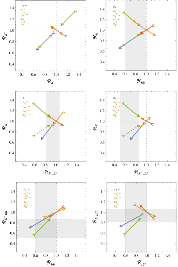
Figure 1: Impact of the Wilson coefficients of the SM-EFT varied within their 2σ2𝜎2\sigma ranges allowed by the global fit to bsμμ𝑏𝑠𝜇𝜇b\to s\mu\mu data. Blue: 𝒄~𝒁subscriptbold-~𝒄𝒁\tilde{c}_{Z}, yellow: 𝒄~𝒁superscriptsubscriptbold-~𝒄𝒁bold-′\tilde{c}_{Z}^{\prime}, green: 𝒄~𝒒𝒍(𝟏)superscriptsubscriptbold-~𝒄𝒒𝒍1\tilde{c}_{ql}^{(1)} (solid) or 𝒄~𝒒𝒍(𝟑)superscriptsubscriptbold-~𝒄𝒒𝒍3\tilde{c}_{ql}^{(3)} (dashed), red: 𝒄~𝒅𝒍subscriptbold-~𝒄𝒅𝒍\tilde{c}_{dl}. The arrows point from negative to positive (real) values of the Wilson coefficients. The shaded bands are the 1σ1𝜎1\sigma experimental measurements.

The impact of the real parts of the Wilson coefficients on the observables is visualized in figure 1. The colored arrows in these plots correspond to the 2σ2𝜎2\sigma allowed ranges of the individual Wilson coefficients as in (38), with the direction of the arrow pointing from negative to positive values for the c~isubscript~𝑐𝑖\tilde{c}_{i}. The blue arrows correspond to c~Zsubscript~𝑐𝑍\tilde{c}_{Z}, the yellow ones to c~Zsuperscriptsubscript~𝑐𝑍\tilde{c}_{Z}^{\prime}, the green ones to c~ql(1)superscriptsubscript~𝑐𝑞𝑙1\tilde{c}_{ql}^{(1)} (solid) or c~ql(3)superscriptsubscript~𝑐𝑞𝑙3\tilde{c}_{ql}^{(3)} (dashed), and the red ones to c~dlsubscript~𝑐𝑑𝑙\tilde{c}_{dl}. Apart from Ksubscript𝐾\mathcal{R}_{K} and Ksubscriptsuperscript𝐾\mathcal{R}_{K^{*}}, we also show the impact on the branching ratios of Bsμ+μsubscript𝐵𝑠superscript𝜇superscript𝜇B_{s}\to\mu^{+}\mu^{-} as well as of BKμ+μ𝐵𝐾superscript𝜇superscript𝜇B\to K\mu^{+}\mu^{-} and BKμ+μ𝐵superscript𝐾superscript𝜇superscript𝜇B\to K^{*}\mu^{+}\mu^{-} at high q2superscript𝑞2q^{2}, defined as

μμsubscript𝜇𝜇\displaystyle\mathcal{R}_{\mu\mu} =BR(Bsμ+μ)BR(Bsμ+μ)SM,absentBRsubscript𝐵𝑠superscript𝜇superscript𝜇BRsubscriptsubscript𝐵𝑠superscript𝜇superscript𝜇SM\displaystyle=\frac{\text{BR}(B_{s}\to\mu^{+}\mu^{-})}{\text{BR}(B_{s}\to\mu^{+}\mu^{-})_{\text{SM}}}\,, (39)
Kμμsubscript𝐾𝜇𝜇\displaystyle\mathcal{R}_{K\mu\mu} =BR(B+K+μ+μ)[15,22]BR(B+K+μ+μ)SM[15,22],absentBRsuperscriptsuperscript𝐵superscript𝐾superscript𝜇superscript𝜇1522BRsubscriptsuperscriptsuperscript𝐵superscript𝐾superscript𝜇superscript𝜇1522SM\displaystyle=\frac{\text{BR}(B^{+}\to K^{+}\mu^{+}\mu^{-})^{[15,22]}}{\text{BR}(B^{+}\to K^{+}\mu^{+}\mu^{-})^{[15,22]}_{\text{SM}}}\,, (40)
Kμμsubscriptsuperscript𝐾𝜇𝜇\displaystyle\mathcal{R}_{K^{*}\mu\mu} =BR(B0K0μ+μ)[15,19]BR(B0K0μ+μ)SM[15,19],absentBRsuperscriptsuperscript𝐵0superscript𝐾absent0superscript𝜇superscript𝜇1519BRsubscriptsuperscriptsuperscript𝐵0superscript𝐾absent0superscript𝜇superscript𝜇1519SM\displaystyle=\frac{\text{BR}(B^{0}\to K^{*0}\mu^{+}\mu^{-})^{[15,19]}}{\text{BR}(B^{0}\to K^{*0}\mu^{+}\mu^{-})^{[15,19]}_{\text{SM}}}\,, (41)

where the superscripts refer to the range in q2superscript𝑞2q^{2} in GeV2. The shaded regions show the values allowed by direct experimental measurements at 1σ1𝜎1\sigma. We make the following observations.

  • The current data on bsμ+μ𝑏𝑠superscript𝜇superscript𝜇b\to s\mu^{+}\mu^{-} processes favour a negative c~ql(1)superscriptsubscript~𝑐𝑞𝑙1\tilde{c}_{ql}^{(1)}, which implies an enhancement of BKνν¯𝐵𝐾𝜈¯𝜈B\to K\nu\bar{\nu} and BKνν¯𝐵superscript𝐾𝜈¯𝜈B\to K^{*}\nu\bar{\nu} by up to 30% and a suppression of Bsμ+μsubscript𝐵𝑠superscript𝜇superscript𝜇B_{s}\to\mu^{+}\mu^{-}, BKμ+μ𝐵𝐾superscript𝜇superscript𝜇B\to K\mu^{+}\mu^{-}, and BKμ+μ𝐵superscript𝐾superscript𝜇superscript𝜇B\to K^{*}\mu^{+}\mu^{-}.

  • If there is NP in left-handed Z𝑍Z penguins (i.e. in c~Zsubscript~𝑐𝑍\tilde{c}_{Z}), current data imply a suppression of BKνν¯𝐵𝐾𝜈¯𝜈B\to K\nu\bar{\nu} and BKνν¯𝐵superscript𝐾𝜈¯𝜈B\to K^{*}\nu\bar{\nu} by up to 40%.

  • With NP in right-handed currents, i.e. in c~dlsubscript~𝑐𝑑𝑙\tilde{c}_{dl} or c~Zsuperscriptsubscript~𝑐𝑍\tilde{c}_{Z}^{\prime}, BKνν¯𝐵𝐾𝜈¯𝜈B\to K\nu\bar{\nu} and BKνν¯𝐵superscript𝐾𝜈¯𝜈B\to K^{*}\nu\bar{\nu} can only be modified at the level of ±10%plus-or-minuspercent10\pm 10\%.

Refer to caption
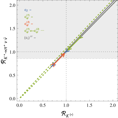
Figure 2: Impact of the Wilson coefficients of the SM-EFT on BK()νν¯𝐵superscript𝐾𝜈¯𝜈B\to K^{(*)}\nu\bar{\nu} vs. K+π+νν¯superscript𝐾superscript𝜋𝜈¯𝜈K^{+}\to\pi^{+}\nu\bar{\nu}, assuming MFV and LFU, varied within their 2σ2𝜎2\sigma ranges allowed by the global fit to bsμμ𝑏𝑠𝜇𝜇b\to s\mu\mu data. Blue: 𝒄~𝒁subscriptbold-~𝒄𝒁\tilde{c}_{Z}, green: 𝒄~𝒒𝒍(𝟏)superscriptsubscriptbold-~𝒄𝒒𝒍1\tilde{c}_{ql}^{(1)}, red: 𝒄~𝒒𝒍(𝟑)superscriptsubscriptbold-~𝒄𝒒𝒍3\tilde{c}_{ql}^{(3)}. The dashed green line shows the case c~ql(1)=c~ql(3)superscriptsubscript~𝑐𝑞𝑙1superscriptsubscript~𝑐𝑞𝑙3\tilde{c}_{ql}^{(1)}=-\tilde{c}_{ql}^{(3)}, where bsμμ𝑏𝑠𝜇𝜇b\to s\mu\mu constraints are ineffective. The gray line corresponds to NP in operators with tau neutrinos only, where K()>2/3superscriptsubscript𝐾23\mathcal{R}_{K}^{(*)}>2/3 (see section 3.4). The shaded band is the 1σ1𝜎1\sigma experimental measurement [48].

3.3.3 The case of Minimal Flavour Violation (MFV)

An interesting special case is MFV, where only the Wilson coefficients c~ql(1,3)superscriptsubscript~𝑐𝑞𝑙13\tilde{c}_{ql}^{(1,3)}, c~qesubscript~𝑐𝑞𝑒\tilde{c}_{qe}, and c~Zsubscript~𝑐𝑍\tilde{c}_{Z} are allowed and are real. Moreover, the same Wilson coefficients c~isubscript~𝑐𝑖\tilde{c}_{i} also enter sdνν¯𝑠𝑑𝜈¯𝜈s\to d\nu\bar{\nu} transitions implying strict correlations between the latter processes and the ones considered here [49]. As the precise rate for K+π+νν¯superscript𝐾superscript𝜋𝜈¯𝜈K^{+}\to\pi^{+}\nu\bar{\nu} is expected to be known before the ones for BK()νν¯𝐵superscript𝐾𝜈¯𝜈B\to K^{(*)}\nu\bar{\nu}, additional constraints on the latter decays will follow in addition to the ones from bs+𝑏𝑠superscriptsuperscriptb\to s\ell^{+}\ell^{-} processes considered by us. In figure 2, we show the correlation between BKνν¯𝐵𝐾𝜈¯𝜈B\to K\nu\bar{\nu} and K+π+νν¯superscript𝐾superscript𝜋𝜈¯𝜈K^{+}\to\pi^{+}\nu\bar{\nu}, normalized to their SM values. As K=Ksubscriptsuperscript𝐾subscript𝐾\mathcal{R}_{K^{*}}=\mathcal{R}_{K} in this framework, the same correlation applies to BKνν¯𝐵superscript𝐾𝜈¯𝜈B\to K^{*}\nu\bar{\nu}.

When varied separately, with bs+𝑏𝑠superscriptsuperscriptb\to s\ell^{+}\ell^{-} constraints taken into account, the above Wilson coefficients lead to deviations of up to ±30%plus-or-minuspercent30\pm 30\% from the SM branching ratios. Very large effects can be obtained in principle in models where c~ql(1)=c~ql(3)superscriptsubscript~𝑐𝑞𝑙1superscriptsubscript~𝑐𝑞𝑙3\tilde{c}_{ql}^{(1)}=-\tilde{c}_{ql}^{(3)}, so contributions to bs+𝑏𝑠superscriptsuperscriptb\to s\ell^{+}\ell^{-} processes vanish and only present weak constraint from K+π+νν¯superscript𝐾superscript𝜋𝜈¯𝜈K^{+}\to\pi^{+}\nu\bar{\nu} play a role. Once the rate for K+π+νν¯superscript𝐾superscript𝜋𝜈¯𝜈K^{+}\to\pi^{+}\nu\bar{\nu} will be experimentally known with a high precision, it will be possible to obtain the allowed region for K=Ksubscriptsuperscript𝐾subscript𝐾\mathcal{R}_{K^{*}}=\mathcal{R}_{K} with the same precision under the assumption of MFV, thereby selecting the favourite MFV models. Eventually one would hope to find the experimental allowed region in the plot in figure 2 to be outside the straight line. This would be an important signal of non-MFV interactions at work, in particular in view of the fact that all processes involved belong to the theoretically cleanest in the field of rare decays. Additional important information will come from CP-violating decay KLπ0νν¯subscript𝐾𝐿superscript𝜋0𝜈¯𝜈K_{L}\to\pi^{0}\nu\bar{\nu} but this will take more time.

3.3.4 Z contributions vs. 4-fermion operators
Refer to caption
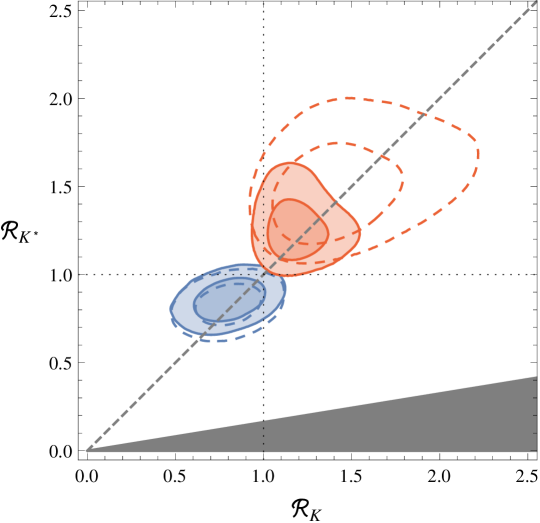
Figure 3: Constraints on the branching ratios of BKνν¯𝐵𝐾𝜈¯𝜈B\to K\nu\bar{\nu} and BKνν¯𝐵superscript𝐾𝜈¯𝜈B\to K^{*}\nu\bar{\nu} normalized to their SM values from a global analysis of bsμ+μ𝑏𝑠superscript𝜇superscript𝜇b\to s\mu^{+}\mu^{-} processes. Blue: assuming NP in in flavour-changing Z𝑍Z couplings only, with real (solid) or complex (dashed) Wilson coefficients. Red: assuming NP in 4-fermion operators only (as happens if the NP contributions are dominated by a SM-singlet Zsuperscript𝑍Z^{\prime}, see sec. 4.1.), with real (solid) or complex (dashed) Wilson coefficients, assuming LFU.

Even if NP contributes to more than one coefficient, there are scenarios in which the NP effects in bsνν¯𝑏𝑠𝜈¯𝜈b\to s\nu\bar{\nu} are quite limited. We now consider the case where NP contributes only through (tree-level or loop-induced) flavour-changing Z𝑍Z couplings, i.e. through c~Zsubscript~𝑐𝑍\tilde{c}_{Z} and c~Zsuperscriptsubscript~𝑐𝑍\tilde{c}_{Z}^{\prime}. To determine the allowed size of the observables, we performed a Markov Chain Monte Carlo scan of the Wilson coefficients c~Zsubscript~𝑐𝑍\tilde{c}_{Z} and c~Zsuperscriptsubscript~𝑐𝑍\tilde{c}_{Z}^{\prime}, assuming flat priors for them. The resulting allowed region in the Ksubscript𝐾\mathcal{R}_{K}-Ksubscriptsuperscript𝐾\mathcal{R}_{K^{*}} plane is shown in figure 3 for real Wilson coefficients (solid blue contours, corresponding to contributions aligned in phase with the SM) as well as for complex Wilson coefficients (dashed blue contours, corresponding to new sources of CP violation).

An orthogonal possibility is to have NP contributions only in Wilson coefficients of 4-fermion operators444Using this terminology we distinguish these contributions from the ones coming from Z𝑍Z contributions even if the latter ones generate at low energies 4-fermion operators., i.e. in c~ql(1)superscriptsubscript~𝑐𝑞𝑙1\tilde{c}_{ql}^{(1)}, c~qesubscript~𝑐𝑞𝑒\tilde{c}_{qe}, c~dlsubscript~𝑐𝑑𝑙\tilde{c}_{dl}, and c~desubscript~𝑐𝑑𝑒\tilde{c}_{de} (but not c~ql(3)superscriptsubscript~𝑐𝑞𝑙3\tilde{c}_{ql}^{(3)}, which is unconstrained as discussed above), which is what happens if the new physics contributions are dominated by a single SM-singlet Zsuperscript𝑍Z^{\prime} gauge boson, as will be discussed in section 4.1. Again, we show the allowed region in the Ksubscript𝐾\mathcal{R}_{K}-Ksubscriptsuperscript𝐾\mathcal{R}_{K^{*}} plane for real or complex Wilson coefficients as solid and dashed red contours in figure 3.

The striking feature of figure 3 is that the current data on bsμ+μ𝑏𝑠superscript𝜇superscript𝜇b\to s\mu^{+}\mu^{-} transitions show some tension with the SM predictions; solving these tensions via Z𝑍Z penguins or via four-fermion operators in the SM-EFT leads to very different predictions for BKνν¯𝐵𝐾𝜈¯𝜈B\to K\nu\bar{\nu} and BKνν¯𝐵superscript𝐾𝜈¯𝜈B\to K^{*}\nu\bar{\nu}. In the former case, a suppression is predicted, in the latter an enhancement (that, for complex coefficients, even comes close to saturating the current experimental bound of K<4.3subscript𝐾4.3\mathcal{R}_{K}<4.3). Needless to say, the tensions in bsμ+μ𝑏𝑠superscript𝜇superscript𝜇b\to s\mu^{+}\mu^{-} data might be due to statistical fluctuations or underestimated uncertainties, but we find it interesting that a measurement of BKνν¯𝐵𝐾𝜈¯𝜈B\to K\nu\bar{\nu} and BKνν¯𝐵superscript𝐾𝜈¯𝜈B\to K^{*}\nu\bar{\nu} could help pin down the source of NP contributions.

3.4 Beyond lepton flavour universality

So far, we have assumed the Wilson coefficients to be independent of the lepton flavour. In general however, they could be different for different lepton flavours while still being lepton flavour conserving – we call this lepton flavour non-universality (LFNU) – and there could even be lepton flavour violation (LFV). In this section, we discuss the implications of these two scenarios for bsνν¯𝑏𝑠𝜈¯𝜈b\to s\nu\bar{\nu}.

3.4.1 LFNU

In the case of LFNU, the Wilson coefficients in the low-energy effective theory get an index =e,μ,τ𝑒𝜇𝜏\ell=e,\mu,\tau distinguishing the neutrino flavour,

𝒪Lsuperscriptsubscript𝒪𝐿\displaystyle\mathcal{O}_{L}^{\ell} =e216π2(s¯γμPLb)(ν¯γμ(1γ5)ν),absentsuperscript𝑒216superscript𝜋2¯𝑠subscript𝛾𝜇subscript𝑃𝐿𝑏¯subscript𝜈superscript𝛾𝜇1subscript𝛾5subscript𝜈\displaystyle=\frac{e^{2}}{16\pi^{2}}(\bar{s}\gamma_{\mu}P_{L}b)(\bar{\nu_{\ell}}\gamma^{\mu}(1-\gamma_{5})\nu_{\ell})\,, 𝒪Rsuperscriptsubscript𝒪𝑅\displaystyle\mathcal{O}_{R}^{\ell} =e216π2(s¯γμPRb)(ν¯γμ(1γ5)ν).absentsuperscript𝑒216superscript𝜋2¯𝑠subscript𝛾𝜇subscript𝑃𝑅𝑏¯subscript𝜈superscript𝛾𝜇1subscript𝛾5subscript𝜈\displaystyle=\frac{e^{2}}{16\pi^{2}}(\bar{s}\gamma_{\mu}P_{R}b)(\bar{\nu_{\ell}}\gamma^{\mu}(1-\gamma_{5})\nu_{\ell})\,. (42)

Defining

ϵ=|CL|2+|CR|2|CLSM|,η=Re(CLCR)|CL|2+|CR|2,formulae-sequencesubscriptitalic-ϵsuperscriptsuperscriptsubscript𝐶𝐿2superscriptsuperscriptsubscript𝐶𝑅2superscriptsubscript𝐶𝐿SMsubscript𝜂Resuperscriptsubscript𝐶𝐿superscriptsubscript𝐶𝑅superscriptsuperscriptsubscript𝐶𝐿2superscriptsuperscriptsubscript𝐶𝑅2\epsilon_{\ell}=\frac{\sqrt{|C_{L}^{\ell}|^{2}+|C_{R}^{\ell}|^{2}}}{|C_{L}^{\text{SM}}|}\leavevmode\nobreak\ ,\qquad\eta_{\ell}=\frac{-\text{Re}\left(C_{L}^{\ell}C_{R}^{\ell*}\right)}{|C_{L}^{\ell}|^{2}+|C_{R}^{\ell}|^{2}}\leavevmode\nobreak\ , (43)

in analogy to (43), the generalization of (20) reads

KKKSMsubscript𝐾subscript𝐾superscriptsubscript𝐾SM\displaystyle\mathcal{R}_{K}\equiv\frac{\mathcal{B}_{K}}{\mathcal{B}_{K}^{\text{SM}}} =13(12η)ϵ2,absent13subscript12subscript𝜂superscriptsubscriptitalic-ϵ2\displaystyle=\frac{1}{3}\sum_{\ell}(1-2\,\eta_{\ell})\epsilon_{\ell}^{2}\,, (44)
KKKSMsubscriptsuperscript𝐾subscriptsuperscript𝐾superscriptsubscriptsuperscript𝐾SM\displaystyle\mathcal{R}_{K^{*}}\equiv\frac{\mathcal{B}_{K^{*}}}{\mathcal{B}_{K^{*}}^{\text{SM}}} =13(1+κηη)ϵ2,absent13subscript1subscript𝜅𝜂subscript𝜂superscriptsubscriptitalic-ϵ2\displaystyle=\frac{1}{3}\sum_{\ell}(1+\kappa_{\eta}\eta_{\ell})\epsilon_{\ell}^{2}\,, (45)
FLFLFLSMsubscriptsubscript𝐹𝐿subscript𝐹𝐿superscriptsubscript𝐹𝐿SM\displaystyle\mathcal{R}_{F_{L}}\equiv\frac{F_{L}}{F_{L}^{\text{SM}}} =ϵ2(1+2η)ϵ2(1+κηη).absentsubscriptsuperscriptsubscriptitalic-ϵ212subscript𝜂subscriptsuperscriptsubscriptitalic-ϵ21subscript𝜅𝜂subscript𝜂\displaystyle=\frac{\sum_{\ell}\epsilon_{\ell}^{2}(1+2\,\eta_{\ell})}{\sum_{\ell}\epsilon_{\ell}^{2}(1+\kappa_{\eta}\eta_{\ell})}\,. (46)

One can check that the model-independent relations (21) and (22) still hold. If NP only contributes to operators involving one of the three lepton flavours, one obtains model-independent lower bounds K>2/3subscript𝐾23\mathcal{R}_{K}>2/3, K>2/3subscriptsuperscript𝐾23\mathcal{R}_{K^{*}}>2/3.

Also the SM-EFT analysis of section 3.2 can be generalized to the case of LFNU. Since the effective Wilson coefficients c~Z()superscriptsubscript~𝑐𝑍\tilde{c}_{Z}^{(\prime)} arise from operators not involving lepton fields at all, their effects are always lepton flavour universal and the bounds in (38) still apply.

The Wilson coefficient of the four-fermion operators instead become lepton flavour dependent and we discuss effects due to operators only involving electrons, muons or taus (and their respective neutrinos) in turn.555As in the LFU case, NP entering the combination (c~ql(1))(c~ql(3))superscriptsuperscriptsubscript~𝑐𝑞𝑙1superscriptsuperscriptsubscript~𝑐𝑞𝑙3(\widetilde{c}_{ql}^{(1)})^{\ell}-(\widetilde{c}_{ql}^{(3)})^{\ell} but not (c~ql(1))+(c~ql(3))superscriptsuperscriptsubscript~𝑐𝑞𝑙1superscriptsuperscriptsubscript~𝑐𝑞𝑙3(\widetilde{c}_{ql}^{(1)})^{\ell}+(\widetilde{c}_{ql}^{(3)})^{\ell} is unconstrained by bs+𝑏𝑠superscriptsuperscriptb\to s\ell^{+}\ell^{-} processes and can in principle give rise to large effects in bsνν¯𝑏𝑠𝜈¯𝜈b\to s\nu\bar{\nu}.

=𝝁bold-ℓ𝝁\ell=\mu

The constraints on the Wilson coefficients of the four-fermion operators involving muon fields, (c~ql(1))μ+(c~ql(3))μsuperscriptsuperscriptsubscript~𝑐𝑞𝑙1𝜇superscriptsuperscriptsubscript~𝑐𝑞𝑙3𝜇(\widetilde{c}_{ql}^{(1)})^{\mu}+(\widetilde{c}_{ql}^{(3)})^{\mu}, (cqe)μsuperscriptsubscript𝑐𝑞𝑒𝜇(c_{qe})^{\mu}, (cdl)μsuperscriptsubscript𝑐𝑑𝑙𝜇(c_{dl})^{\mu}, and (cde)μsuperscriptsubscript𝑐𝑑𝑒𝜇(c_{de})^{\mu}, are the same as the LFU scenario considered in section 3.3, since we considered only constraints from decays involving muons in the final state. However, the deviations from the SM in BK()νν¯𝐵superscript𝐾𝜈¯𝜈B\to K^{(*)}\nu\bar{\nu} are now a factor of 1313\frac{1}{3} smaller, since only muon neutrinos contribute. The allowed region in the Ksubscript𝐾\mathcal{R}_{K}-Ksubscriptsuperscript𝐾\mathcal{R}_{K^{*}} plane in figure 3, shown in red, would thus shrink by this factor (in a geometrically similar way, i.e. without changing its shape). We note that the case with NP in =μ𝜇\ell=\mu only is particularly interesting in view of the recent measurement by LHCb of the ratio of the BKe+e𝐵𝐾superscript𝑒superscript𝑒B\to Ke^{+}e^{-} to BKμ+μ𝐵𝐾superscript𝜇superscript𝜇B\to K\mu^{+}\mu^{-} branching ratios at low q2superscript𝑞2q^{2}, found to deviate from LFU by 2.6σ2.6𝜎2.6\sigma [50] (see also [10]).

=𝝉bold-ℓ𝝉\ell=\tau

For four-fermion operators involving taus, constraints from semi-leptonic FCNCs are more than two orders of magnitude weaker than for muons [51]. Consequently, the effects in bsνν¯𝑏𝑠𝜈¯𝜈b\to s\nu\bar{\nu} decays could easily saturate the experimental upper bounds. In fact, the current upper bounds on the BK()νν¯𝐵superscript𝐾𝜈¯𝜈B\to K^{(*)}\nu\bar{\nu} branching ratios represent the most stringent bounds on FCNC operators in the SM-EFT involving left-handed tau leptons and limit the size of NP effects that can be generated in bsτ+τ𝑏𝑠superscript𝜏superscript𝜏b\to s\tau^{+}\tau^{-} decays from these operators.

=𝒆bold-ℓ𝒆\ell=e

In the case of four-fermion operators involving electron fields, the only constraints at present are the branching ratio of the inclusive BXse+e𝐵subscript𝑋𝑠superscript𝑒superscript𝑒B\to X_{s}e^{+}e^{-} decay measured by BaBar [52] as well the branching ratio of B+K+e+esuperscript𝐵superscript𝐾superscript𝑒superscript𝑒B^{+}\to K^{+}e^{+}e^{-} measured recently by LHCb [50]. Using these measurements, we obtain the following 2σ2𝜎2\sigma allowed ranges for the Wilson coefficients,

Re(c~ql(1)+c~ql(3))Resuperscriptsubscript~𝑐𝑞𝑙1superscriptsubscript~𝑐𝑞𝑙3\displaystyle\text{Re}(\tilde{c}_{ql}^{(1)}+\tilde{c}_{ql}^{(3)}) [0.42,+0.92]absent0.420.92\displaystyle\in[-0.42,+0.92] Im(c~ql(1)+c~ql(3))Imsuperscriptsubscript~𝑐𝑞𝑙1superscriptsubscript~𝑐𝑞𝑙3\displaystyle\text{Im}(\tilde{c}_{ql}^{(1)}+\tilde{c}_{ql}^{(3)}) [2.9,+2.9]absent2.92.9\displaystyle\in[-2.9,+2.9] (47)
Rec~dlResubscript~𝑐𝑑𝑙\displaystyle\text{Re}\,\tilde{c}_{dl} [0.83,+0.91]absent0.830.91\displaystyle\in[-0.83,+0.91] Imc~dlImsubscript~𝑐𝑑𝑙\displaystyle\text{Im}\,\tilde{c}_{dl} [2.9,+2.9]absent2.92.9\displaystyle\in[-2.9,+2.9] (48)
Rec~ZResubscript~𝑐𝑍\displaystyle\text{Re}\,\tilde{c}_{Z} [1.6,+0.8]absent1.60.8\displaystyle\in[-1.6,+0.8] Imc~ZImsubscript~𝑐𝑍\displaystyle\text{Im}\,\tilde{c}_{Z} [4.0,+4.0]absent4.04.0\displaystyle\in[-4.0,+4.0] (49)
Rec~ZResuperscriptsubscript~𝑐𝑍\displaystyle\text{Re}\,\tilde{c}_{Z}^{\prime} [1.6,+1.8]absent1.61.8\displaystyle\in[-1.6,+1.8] Imc~ZImsuperscriptsubscript~𝑐𝑍\displaystyle\text{Im}\,\tilde{c}_{Z}^{\prime} [4.0,+4.0]absent4.04.0\displaystyle\in[-4.0,+4.0] (50)

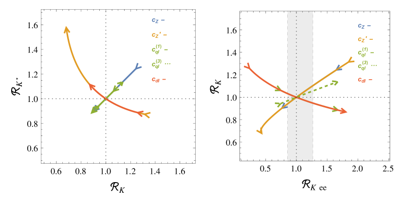
These bounds are significantly looser than in the LFU case (38), so in spite of the fact that the effects in the BK()νν¯𝐵superscript𝐾𝜈¯𝜈B\to K^{(*)}\nu\bar{\nu} branching ratios are a factor of 3 smaller, since only one neutrino flavour contributes, the allowed effects can be bigger. This is visualized in figure 4, showing in analogy to figure 1 the correlation between Ksubscript𝐾\mathcal{R}_{K} and Ksubscriptsuperscript𝐾\mathcal{R}_{K^{*}} as well as between Ksubscript𝐾\mathcal{R}_{K} and the low-q2superscript𝑞2q^{2} branching ratio

Kee=BR(B+K+e+e)[1,6]BR(B+K+e+e)SM[1,6].subscript𝐾𝑒𝑒BRsuperscriptsuperscript𝐵superscript𝐾superscript𝑒superscript𝑒16BRsubscriptsuperscriptsuperscript𝐵superscript𝐾superscript𝑒superscript𝑒16SM\mathcal{R}_{Kee}=\frac{\text{BR}(B^{+}\to K^{+}e^{+}e^{-})^{[1,6]}}{\text{BR}(B^{+}\to K^{+}e^{+}e^{-})^{[1,6]}_{\text{SM}}}\,. (51)
Refer to caption
Figure 4: Impact of the Wilson coefficients of the SM-EFT varied within their 2σ2𝜎2\sigma ranges, assuming coefficients with electrons only, as allowed by a fit to bse+e𝑏𝑠superscript𝑒superscript𝑒b\to se^{+}e^{-} data. Colors as in figure 1.

3.4.2 LFV

In general, the operators in the low-energy Hamiltonian could violate lepton flavour,

𝒪Lijsuperscriptsubscript𝒪𝐿𝑖𝑗\displaystyle\mathcal{O}_{L}^{ij} =e216π2(s¯γμPLb)(νi¯γμ(1γ5)νj),absentsuperscript𝑒216superscript𝜋2¯𝑠subscript𝛾𝜇subscript𝑃𝐿𝑏¯subscript𝜈𝑖superscript𝛾𝜇1subscript𝛾5subscript𝜈𝑗\displaystyle=\frac{e^{2}}{16\pi^{2}}(\bar{s}\gamma_{\mu}P_{L}b)(\bar{\nu_{i}}\gamma^{\mu}(1-\gamma_{5})\nu_{j})\,, 𝒪Rijsuperscriptsubscript𝒪𝑅𝑖𝑗\displaystyle\mathcal{O}_{R}^{ij} =e216π2(s¯γμPRb)(νi¯γμ(1γ5)νj),absentsuperscript𝑒216superscript𝜋2¯𝑠subscript𝛾𝜇subscript𝑃𝑅𝑏¯subscript𝜈𝑖superscript𝛾𝜇1subscript𝛾5subscript𝜈𝑗\displaystyle=\frac{e^{2}}{16\pi^{2}}(\bar{s}\gamma_{\mu}P_{R}b)(\bar{\nu_{i}}\gamma^{\mu}(1-\gamma_{5})\nu_{j})\,, (52)

with ij𝑖𝑗i\neq j. In analogy to the case of LFNU, one can now define

ϵij=|CLij|2+|CRij|2|CLSM|,ηij=Re(CLijCRij)|CLij|2+|CRij|2,formulae-sequencesubscriptitalic-ϵ𝑖𝑗superscriptsuperscriptsubscript𝐶𝐿𝑖𝑗2superscriptsuperscriptsubscript𝐶𝑅𝑖𝑗2superscriptsubscript𝐶𝐿SMsubscript𝜂𝑖𝑗Resuperscriptsubscript𝐶𝐿𝑖𝑗superscriptsubscript𝐶𝑅𝑖𝑗superscriptsuperscriptsubscript𝐶𝐿𝑖𝑗2superscriptsuperscriptsubscript𝐶𝑅𝑖𝑗2\epsilon_{ij}=\frac{\sqrt{|C_{L}^{ij}|^{2}+|C_{R}^{ij}|^{2}}}{|C_{L}^{\text{SM}}|}\leavevmode\nobreak\ ,\qquad\eta_{ij}=\frac{-\text{Re}\left(C_{L}^{ij}C_{R}^{{ij}*}\right)}{|C_{L}^{ij}|^{2}+|C_{R}^{ij}|^{2}}\leavevmode\nobreak\ , (53)

and (46) still hold with the replacements ϵ,ηsubscriptitalic-ϵsubscript𝜂\epsilon_{\ell},\eta_{\ell} \to ϵij,ηijsubscriptitalic-ϵ𝑖𝑗subscript𝜂𝑖𝑗\epsilon_{ij},\eta_{ij}. Note that in the SM, ϵij=0subscriptitalic-ϵ𝑖𝑗0\epsilon_{ij}=0 for ij𝑖𝑗i\neq j. It is now easy to see that the model-independent relations (21) and (22) still hold.

Only few searches for LFV B𝐵B decays exist. The most stringent bound on LFV operators in the SM-EFT comes from the recent search for Bseμsubscript𝐵𝑠𝑒𝜇B_{s}\to e\mu by the LHCb collaboration [53], finding

BR(Bse±μ)<1.4×10⁸BRsubscript𝐵𝑠superscript𝑒plus-or-minussuperscript𝜇minus-or-plus1.4superscript108\text{BR}(B_{s}\to e^{\pm}\mu^{\mp})<1.4\times 10^{-8} (54)

at 95% confidence level. This implies

|(C9)μe(C9)μe|2+|(C10)μe(C10)μe|2<16.62superscriptsuperscriptsubscript𝐶9𝜇𝑒superscriptsuperscriptsubscript𝐶9𝜇𝑒2superscriptsuperscriptsubscript𝐶10𝜇𝑒superscriptsuperscriptsubscript𝐶10𝜇𝑒2superscript16.62|(C_{9})^{\mu e}-(C_{9}^{\prime})^{\mu e}|^{2}+|(C_{10})^{\mu e}-(C_{10}^{\prime})^{\mu e}|^{2}<16.6^{2} (55)

and likewise for the (Ci())eμsuperscriptsuperscriptsubscript𝐶𝑖𝑒𝜇(C_{i}^{(\prime)})^{e\mu}. These Wilson coefficients are the obvious generalizations of (31) and (32) for the LFV case and they vanish in the SM. We are not aware of any existing bounds on LFV operators involving tau leptons.

We can now consider as an example a NP effect only in (c~ql(1))eμsuperscriptsuperscriptsubscript~𝑐𝑞𝑙1𝑒𝜇(\widetilde{c}_{ql}^{(1)})^{e\mu}. As there is no interference between the SM and NP contribution in this case, we obtain

K=K=1+13|(c~ql(1))eμ|2|CLSM|2.subscript𝐾subscriptsuperscript𝐾113superscriptsuperscriptsuperscriptsubscript~𝑐𝑞𝑙1𝑒𝜇2superscriptsuperscriptsubscript𝐶𝐿SM2\mathcal{R}_{K}=\mathcal{R}_{K^{*}}=1+\frac{1}{3}\frac{|(\widetilde{c}_{ql}^{(1)})^{e\mu}|^{2}}{|C_{L}^{\text{SM}}|^{2}}\,. (56)

Using next

CLSM=6.35,|(c~ql(1))eμ|11.7,formulae-sequencesuperscriptsubscript𝐶𝐿SM6.35superscriptsuperscriptsubscript~𝑐𝑞𝑙1𝑒𝜇11.7C_{L}^{\text{SM}}=-6.35,\qquad|(\widetilde{c}_{ql}^{(1)})^{e\mu}|\leq 11.7\,, (57)

with the latter bound following from (55), we find

1K=K2.14.1subscript𝐾subscriptsuperscript𝐾2.141\leq\mathcal{R}_{K}=\mathcal{R}_{K^{*}}\leq 2.14\,. (58)

To summarize, a NP contribution to BK()νν¯𝐵superscript𝐾𝜈¯𝜈B\to K^{(*)}\nu\bar{\nu} that is purely LFV

  • always leads to an enhancement of the branching ratios,

  • can lead to a factor of 2 enhancement of K()subscriptsuperscript𝐾\mathcal{R}_{K^{(*)}} for ij=eμ𝑖𝑗𝑒𝜇ij=e\mu, constrained by the search for Bse±μsubscript𝐵𝑠superscript𝑒plus-or-minussuperscript𝜇minus-or-plusB_{s}\to e^{\pm}\mu^{\mp},

  • can saturate the experimental bounds if tau neutrinos are involved.

4 Specific new physics models

4.1 General 𝒁superscript𝒁bold-′\bm{\mathsfit{Z^{\prime}}} Models

We will next consider general Zsuperscript𝑍Z^{\prime} models assuming that NP contributions are dominated by the tree-level exchange of a heavy neutral gauge boson with mass MZsubscript𝑀superscript𝑍M_{Z^{\prime}} that transforms as a singlet under SU(2)L𝑆𝑈subscript2𝐿SU(2)_{L}. The recent detailed analyses of FCNCs in these models can be found in [19, 20, 54]. We will follow the notation of Zsuperscript𝑍Z^{\prime} couplings in these papers,

f¯iγμ[ΔLfifj(Z)PL+ΔRfifj(Z)PR]fjZμ,subscript¯𝑓𝑖superscript𝛾𝜇delimited-[]subscriptsuperscriptΔsubscript𝑓𝑖subscript𝑓𝑗𝐿superscript𝑍subscript𝑃𝐿subscriptsuperscriptΔsubscript𝑓𝑖subscript𝑓𝑗𝑅superscript𝑍subscript𝑃𝑅subscript𝑓𝑗subscriptsuperscript𝑍𝜇\mathcal{L}\supset\bar{f}_{i}\gamma^{\mu}\left[\Delta^{f_{i}f_{j}}_{L}(Z^{\prime})P_{L}+\Delta^{f_{i}f_{j}}_{R}(Z^{\prime})P_{R}\right]f_{j}\,Z^{\prime}_{\mu}\,, (59)

and recall that SU(2)L𝑆𝑈subscript2𝐿SU(2)_{L} symmetry implies ΔLνν¯(Z)=ΔL(Z)superscriptsubscriptΔ𝐿𝜈¯𝜈superscript𝑍superscriptsubscriptΔ𝐿superscript𝑍\Delta_{L}^{\nu\bar{\nu}}(Z^{\prime})=\Delta_{L}^{\ell\ell}(Z^{\prime}). The quark couplings are in general complex whereas the leptonic ones are assumed to be real. This results in the following tree-level contributions to the Wilson coefficients in the SM-EFT,

c~ql(1)superscriptsubscript~𝑐𝑞𝑙1\displaystyle\tilde{c}_{ql}^{(1)} =ΔLsbΔLVtbVts[5TeVMZ]2,absentsubscriptsuperscriptΔ𝑠𝑏𝐿subscriptsuperscriptΔ𝐿subscript𝑉𝑡𝑏superscriptsubscript𝑉𝑡𝑠superscriptdelimited-[]5TeVsubscript𝑀superscript𝑍2\displaystyle=-\frac{\Delta^{sb}_{L}\Delta^{\ell\ell}_{L}}{V_{tb}V_{ts}^{*}}\left[\frac{5\,\text{TeV}}{M_{Z^{\prime}}}\right]^{2}\,, c~dlsubscript~𝑐𝑑𝑙\displaystyle\tilde{c}_{dl} =ΔRsbΔLVtbVts[5TeVMZ]2,absentsubscriptsuperscriptΔ𝑠𝑏𝑅subscriptsuperscriptΔ𝐿subscript𝑉𝑡𝑏superscriptsubscript𝑉𝑡𝑠superscriptdelimited-[]5TeVsubscript𝑀superscript𝑍2\displaystyle=-\frac{\Delta^{sb}_{R}\Delta^{\ell\ell}_{L}}{V_{tb}V_{ts}^{*}}\left[\frac{5\,\text{TeV}}{M_{Z^{\prime}}}\right]^{2}\,, (60)
c~qesubscript~𝑐𝑞𝑒\displaystyle\tilde{c}_{qe} =ΔLsbΔRVtbVts[5TeVMZ]2,absentsubscriptsuperscriptΔ𝑠𝑏𝐿subscriptsuperscriptΔ𝑅subscript𝑉𝑡𝑏superscriptsubscript𝑉𝑡𝑠superscriptdelimited-[]5TeVsubscript𝑀superscript𝑍2\displaystyle=-\frac{\Delta^{sb}_{L}\Delta^{\ell\ell}_{R}}{V_{tb}V_{ts}^{*}}\left[\frac{5\,\text{TeV}}{M_{Z^{\prime}}}\right]^{2}\,, c~desubscript~𝑐𝑑𝑒\displaystyle\tilde{c}_{de} =ΔRsbΔRVtbVts[5TeVMZ]2,absentsubscriptsuperscriptΔ𝑠𝑏𝑅subscriptsuperscriptΔ𝑅subscript𝑉𝑡𝑏superscriptsubscript𝑉𝑡𝑠superscriptdelimited-[]5TeVsubscript𝑀superscript𝑍2\displaystyle=-\frac{\Delta^{sb}_{R}\Delta^{\ell\ell}_{R}}{V_{tb}V_{ts}^{*}}\left[\frac{5\,\text{TeV}}{M_{Z^{\prime}}}\right]^{2}\,, (61)

where the 5 TeV stem from (29). Here we have again assumed LFU. In that case, the lepton couplings are constrained from LEP2 searches for contact interactions [55, 56],

|ΔL|MZsubscriptsuperscriptΔ𝐿subscript𝑀superscript𝑍\displaystyle\frac{|\Delta^{\ell\ell}_{L}|}{M_{Z^{\prime}}} <0.41TeV,absent0.41TeV\displaystyle<\frac{0.41}{\text{TeV}}\,, |ΔR|MZsubscriptsuperscriptΔ𝑅subscript𝑀superscript𝑍\displaystyle\frac{|\Delta^{\ell\ell}_{R}|}{M_{Z^{\prime}}} <0.44TeV.absent0.44TeV\displaystyle<\frac{0.44}{\text{TeV}}\,. (62)

The quark couplings are in general complex. The mass difference in Bssubscript𝐵𝑠B_{s}-B¯ssubscript¯𝐵𝑠\bar{B}_{s} mixing leads to the constraint

1MZ2|(ΔLbs)2+(ΔRbs)28.6ΔLbsΔRbs|<(0.004TeV)2,1superscriptsubscript𝑀superscript𝑍2superscriptsubscriptsuperscriptΔ𝑏𝑠𝐿2superscriptsubscriptsuperscriptΔ𝑏𝑠𝑅28.6subscriptsuperscriptΔ𝑏𝑠𝐿subscriptsuperscriptΔ𝑏𝑠𝑅superscript0.004TeV2\displaystyle\frac{1}{M_{Z^{\prime}}^{2}}\left|(\Delta^{bs}_{L})^{2}+(\Delta^{bs}_{R})^{2}-8.6\,\Delta^{bs}_{L}\Delta^{bs}_{R}\right|<\left(\frac{0.004}{\text{TeV}}\right)^{2}\,, (63)

where the numerical factor 8.68.68.6 corresponds to MZ=5TeVsubscript𝑀superscript𝑍5TeVM_{Z^{\prime}}=5\,\text{TeV}. It increases logarithmically with MZsubscript𝑀superscript𝑍M_{Z^{\prime}} reaching 10.010.010.0 for MZ=20TeVsubscript𝑀superscript𝑍20TeVM_{Z^{\prime}}=20\,\text{TeV}. Details can be found in [54]. Similarly, the measurement of the Bssubscript𝐵𝑠B_{s} mixing phase constrains the argument of the combination of couplings. Since we do not specify the flavour-conserving couplings to first and second generation quarks, we do not need to consider direct LHC bounds or bounds from atomic parity violation.

Allowing the flavour-violating couplings to quarks to be complex, in principle one can arrange for cancellations in the Bssubscript𝐵𝑠B_{s} mixing constraints and obtain large effects in BK()νν¯𝐵superscript𝐾𝜈¯𝜈B\to K^{(*)}\nu\bar{\nu}. Barring such fine-tuned scenarios, it is more instructive to consider several cases for the ratio between left- and right-handed flavour-changing couplings. We will consider four cases: the scenario in which only LH quark couplings are present (LHS), the one with only RH couplings (RHS), the one with LH and RH couplings being equal (LRS) and one with these couplings differing by sign (ALR). We will use the following colour coding for them

LHS=(red),RHS=(blue),LRS=(green),ALRS=(yellow).formulae-sequenceLHS(red)formulae-sequenceRHS(blue)formulae-sequenceLRS(green)ALRS(yellow)\text{LHS}=\text{(red)},\quad\text{RHS}=\text{(blue)},\quad\text{LRS}=\text{(green)},\quad\text{ALRS}=\text{(yellow)}. (64)

Since we are mainly interested in bsνν¯𝑏𝑠𝜈¯𝜈b\to s\nu\bar{\nu} transitions, we consider only Zsuperscript𝑍Z^{\prime} couplings to left-handed leptons,

ΔRνν¯(Z)=ΔR(Z)=0.superscriptsubscriptΔ𝑅𝜈¯𝜈superscript𝑍superscriptsubscriptΔ𝑅superscript𝑍0\Delta_{R}^{\nu\bar{\nu}}(Z^{\prime})=\Delta_{R}^{\ell\ell}(Z^{\prime})=0\,. (65)

The relevant formulae for processes of interest in terms of these couplings are collected in [19, 20] and we will not repeat them here. The ΔF=2Δ𝐹2\Delta F=2 constraint has been incorporated through the conditions

0.14Sψϕ0.14,0.9CBsΔMsΔMsSM1.1.formulae-sequence0.14subscript𝑆𝜓italic-ϕ0.140.9subscript𝐶subscript𝐵𝑠Δsubscript𝑀𝑠Δsuperscriptsubscript𝑀𝑠SM1.1-0.14\leq S_{\psi\phi}\leq 0.14,\qquad 0.9\leq C_{B_{s}}\equiv\frac{\Delta M_{s}}{\Delta M_{s}^{\text{SM}}}\leq 1.1\,. (66)
Refer to caption
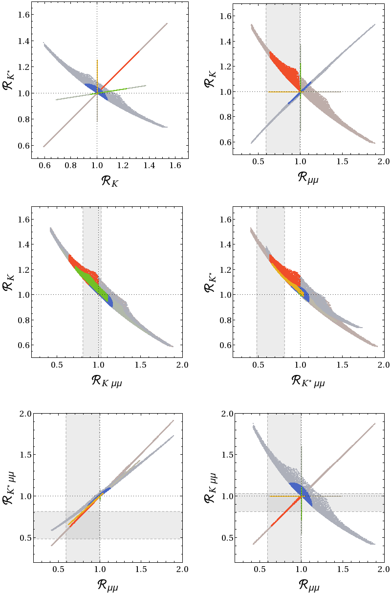
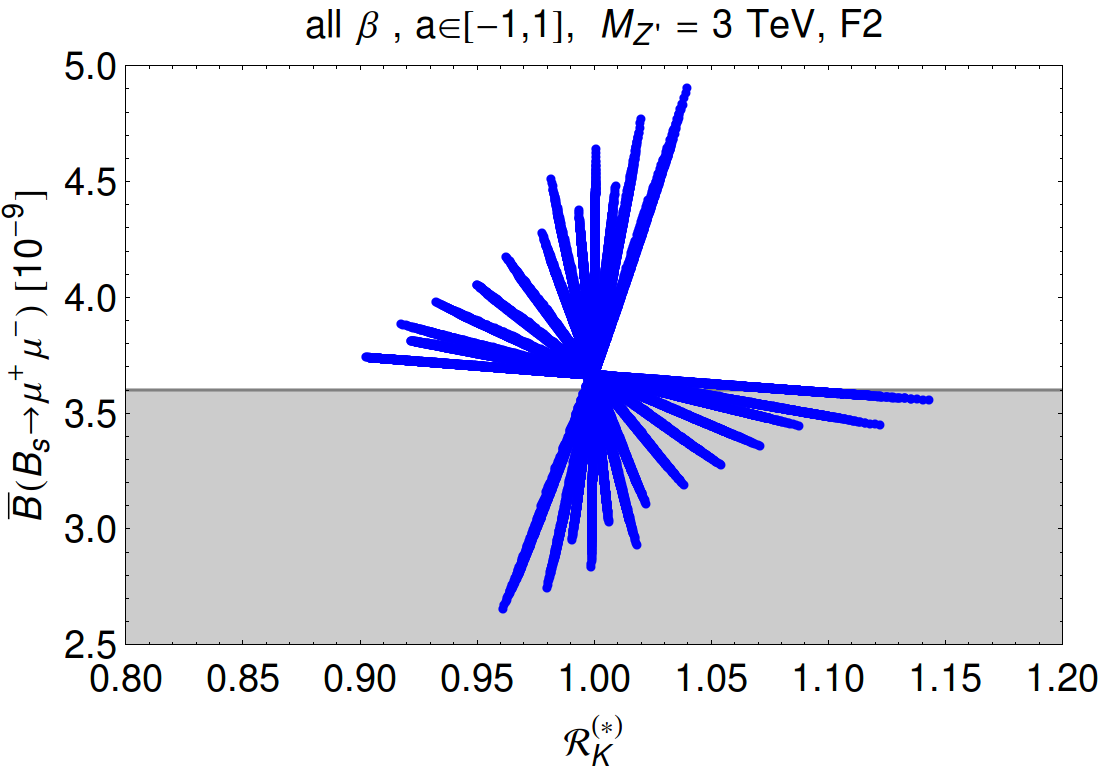
Figure 5: Various correlations between observables in LHS (red), RHS (blue), LRS (green), ALRS (yellow), assuming LFU and ΔRνν=ΔR=0superscriptsubscriptΔ𝑅𝜈𝜈superscriptsubscriptΔ𝑅0\Delta_{R}^{\nu\nu}=\Delta_{R}^{\ell\ell}=0. All points satisfy 0.9CBs1.10.9subscript𝐶subscript𝐵𝑠1.10.9\leq C_{B_{s}}\leq 1.1, 0.14Sψϕ0.140.14subscript𝑆𝜓italic-ϕ0.14-0.14\leq S_{\psi\phi}\leq 0.14. Grey regions are disfavoured at 2σ2𝜎2\sigma by bsμ+μ𝑏𝑠superscript𝜇superscript𝜇b\to s\mu^{+}\mu^{-} constraints.

In figure 5 we show the correlations between the same observables as in figure 1. All points fulfill the ΔF=2Δ𝐹2\Delta F=2 constraints. Some of the points passing ΔF=2Δ𝐹2\Delta F=2 constraints are disfavoured by the global analysis of bsμ+μ𝑏𝑠superscript𝜇superscript𝜇b\to s\mu^{+}\mu^{-} data. These are shown as grey regions in the figure. These plots show in a spectacular manner how different scenarios for couplings can be distinguished through correlations. Qualitative understanding of these plots can be gained by inspecting DNA charts in [1] paying attention to the signs of the leptonic couplings as explained there.

Here we just want to emphasize most important points. The choice of the couplings in (65) corresponds to a very simple structure of the Wilson coefficients in the effective theory approach

CLsubscript𝐶𝐿\displaystyle C_{L} =CLSM+c~ql(1),absentsuperscriptsubscript𝐶𝐿SMsuperscriptsubscript~𝑐𝑞𝑙1\displaystyle=C_{L}^{\text{SM}}+\widetilde{c}_{ql}^{(1)}\,, CRsubscript𝐶𝑅\displaystyle C_{R} =c~dl,absentsubscript~𝑐𝑑𝑙\displaystyle=\widetilde{c}_{dl}\,, (67)
C9subscript𝐶9\displaystyle C_{9} =C9SM+c~ql(1),absentsuperscriptsubscript𝐶9SMsuperscriptsubscript~𝑐𝑞𝑙1\displaystyle=C_{9}^{\text{SM}}+\widetilde{c}_{ql}^{(1)}\,, C9superscriptsubscript𝐶9\displaystyle C_{9}^{\prime} =c~dl,absentsubscript~𝑐𝑑𝑙\displaystyle=\widetilde{c}_{dl}\,, (68)
C10subscript𝐶10\displaystyle C_{10} =C10SMc~ql(1),absentsuperscriptsubscript𝐶10SMsuperscriptsubscript~𝑐𝑞𝑙1\displaystyle=C_{10}^{\text{SM}}-\widetilde{c}_{ql}^{(1)}\,, C10superscriptsubscript𝐶10\displaystyle C_{10}^{\prime} =c~dl,absentsubscript~𝑐𝑑𝑙\displaystyle=-\widetilde{c}_{dl}\,, (69)

implying correlations between Wilson coefficients

CLNP=C9NP=C10NP,CR=C9=C10.formulae-sequencesuperscriptsubscript𝐶𝐿NPsuperscriptsubscript𝐶9NPsuperscriptsubscript𝐶10NPsubscript𝐶𝑅superscriptsubscript𝐶9superscriptsubscript𝐶10C_{L}^{\text{NP}}=C_{9}^{\text{NP}}=-C_{10}^{\text{NP}},\qquad C_{R}=C_{9}^{\prime}=-C_{10}^{\prime}. (70)

The relation C9NP=C10NP<0superscriptsubscript𝐶9NPsuperscriptsubscript𝐶10NP0C_{9}^{\text{NP}}=-C_{10}^{\text{NP}}<0 has been recently advocated in [10] as a simple description of the present data on bsμ+μ𝑏𝑠superscript𝜇superscript𝜇b\to s\mu^{+}\mu^{-} transitions.

As a result of these correlations we have the following unique predictions seen in figure 5:

  • In the LHS Ksubscript𝐾\mathcal{R}_{K} and Ksuperscriptsubscript𝐾\mathcal{R}_{K}^{*} are correlated with each other, whereas in the RHS they are anti-correlated.

  • The suppression of the rate for Bsμ+μsubscript𝐵𝑠superscript𝜇superscript𝜇B_{s}\to\mu^{+}\mu^{-} (μμ<1subscript𝜇𝜇1\mathcal{R}_{\mu\mu}<1) relative to its SM value implies the enhancement of Ksubscript𝐾\mathcal{R}_{K} in the LHS and its suppression in the RHS.

  • Ksubscript𝐾\mathcal{R}_{K} is anti-correlated with Kμμsubscript𝐾𝜇𝜇\mathcal{R}_{K\mu\mu} independently of scenario considered. The same applies to the relation between Ksuperscriptsubscript𝐾\mathcal{R}_{K}^{*} and Kμμsubscriptsuperscript𝐾𝜇𝜇\mathcal{R}_{K^{*}\mu\mu}.

  • In accordance with the present data, μμ<1subscript𝜇𝜇1\mathcal{R}_{\mu\mu}<1 implies Kμμ<1subscriptsuperscript𝐾𝜇𝜇1\mathcal{R}_{K^{*}\mu\mu}<1 in all scenarios considered.

  • On the other hand the simultaneous suppression of μμ<1subscript𝜇𝜇1\mathcal{R}_{\mu\mu}<1 and Kμμ<1subscript𝐾𝜇𝜇1\mathcal{R}_{K\mu\mu}<1 observed in the data favours the LHS and strongly disfavours the RHS.

So far, we have assumed LFU. Here, we briefly comment on the Zsuperscript𝑍Z^{\prime} model with gauged muon minus tau lepton number (LμLτ)subscript𝐿𝜇subscript𝐿𝜏(L_{\mu}-L_{\tau}) proposed recently in [57] to address a number of tensions observed in bsμ+μ𝑏𝑠superscript𝜇superscript𝜇b\to s\mu^{+}\mu^{-} transitions. In this model, one has

(c~qe)μμsuperscriptsubscript~𝑐𝑞𝑒𝜇𝜇\displaystyle(\tilde{c}_{qe})^{\mu\mu} =(c~ql(1))μμ=(c~qe)ττ=(c~ql(1))ττ,absentsuperscriptsuperscriptsubscript~𝑐𝑞𝑙1𝜇𝜇superscriptsubscript~𝑐𝑞𝑒𝜏𝜏superscriptsuperscriptsubscript~𝑐𝑞𝑙1𝜏𝜏\displaystyle=(\tilde{c}_{ql}^{(1)})^{\mu\mu}=-(\tilde{c}_{qe})^{\tau\tau}=-(\tilde{c}_{ql}^{(1)})^{\tau\tau}\,, (71)
(c~de)μμsuperscriptsubscript~𝑐𝑑𝑒𝜇𝜇\displaystyle(\tilde{c}_{de})^{\mu\mu} =(c~dl)μμ=(c~de)ττ=(c~dl)ττ.absentsuperscriptsubscript~𝑐𝑑𝑙𝜇𝜇superscriptsubscript~𝑐𝑑𝑒𝜏𝜏superscriptsubscript~𝑐𝑑𝑙𝜏𝜏\displaystyle=(\tilde{c}_{dl})^{\mu\mu}=-(\tilde{c}_{de})^{\tau\tau}=-(\tilde{c}_{dl})^{\tau\tau}\,. (72)

Consequently, the enhancement of the muon neutrino contribution to BK()νν¯𝐵superscript𝐾𝜈¯𝜈B\to K^{(*)}\nu\bar{\nu} is cancelled almost exactly by the suppression of the tau neutrino contribution and the final effect is unobservably small [57].

4.2 331 Models

In the so-called 331 models based on the gauge group SU(3)C×SU(3)L×U(1)X𝑆𝑈subscript3𝐶𝑆𝑈subscript3𝐿𝑈subscript1𝑋SU(3)_{C}\times SU(3)_{L}\times U(1)_{X} FCNC processes receive tree-level contributions from a new heavy neutral gauge boson Zsuperscript𝑍Z^{\prime} and through ZZ𝑍superscript𝑍Z-Z^{\prime} mixing also from tree-level SM Z𝑍Z boson exchanges. In this model, only left-handed quark currents are present so that CRsubscript𝐶𝑅C_{R}, C9superscriptsubscript𝐶9C_{9}^{\prime}, and C10superscriptsubscript𝐶10C_{10}^{\prime} vanish. Moreover, c~ql(3)=0superscriptsubscript~𝑐𝑞𝑙30\widetilde{c}_{ql}^{(3)}=0. For the remaining coefficients of the effective theory, we find:

sin2θWc~ql(1)=[ΔLνν(Z)gSM2MZ2]ΔLqb(Z)VtqVtb,superscript2subscript𝜃𝑊superscriptsubscript~𝑐𝑞𝑙1delimited-[]superscriptsubscriptΔ𝐿𝜈𝜈superscript𝑍subscriptsuperscript𝑔2SMsuperscriptsubscript𝑀superscript𝑍2superscriptsubscriptΔ𝐿𝑞𝑏superscript𝑍superscriptsubscript𝑉𝑡𝑞subscript𝑉𝑡𝑏\sin^{2}\theta_{W}\widetilde{c}_{ql}^{(1)}=-\left[\frac{\Delta_{L}^{\nu\nu}(Z^{\prime})}{g^{2}_{\text{SM}}M_{Z^{\prime}}^{2}}\right]\frac{\Delta_{L}^{qb}(Z^{\prime})}{V_{tq}^{\ast}V_{tb}}\,, (73)
c~Z=RννLc~ql(1),subscript~𝑐𝑍subscriptsuperscript𝑅𝐿𝜈𝜈superscriptsubscript~𝑐𝑞𝑙1\widetilde{c}_{Z}=R^{L}_{\nu\nu}\widetilde{c}_{ql}^{(1)}\,, (74)
sin2θWc~qe=[ΔRμμ(Z)gSM2MZ2]ΔLqb(Z)VtqVtb.superscript2subscript𝜃𝑊subscript~𝑐𝑞𝑒delimited-[]superscriptsubscriptΔ𝑅𝜇𝜇superscript𝑍subscriptsuperscript𝑔2SMsuperscriptsubscript𝑀superscript𝑍2superscriptsubscriptΔ𝐿𝑞𝑏superscript𝑍superscriptsubscript𝑉𝑡𝑞subscript𝑉𝑡𝑏\sin^{2}\theta_{W}\widetilde{c}_{qe}=-\left[\frac{\Delta_{R}^{\mu\mu}(Z^{\prime})}{g^{2}_{\text{SM}}M_{Z^{\prime}}^{2}}\right]\frac{\Delta_{L}^{qb}(Z^{\prime})}{V_{tq}^{\ast}V_{tb}}\,. (75)

where ΔL,Rij(Z)superscriptsubscriptΔ𝐿𝑅𝑖𝑗superscript𝑍\Delta_{L,R}^{ij}(Z^{\prime}) are the couplings defined in [24],

gSM2=4GF2α2πsin2θW=1.78137×10⁷GeV2,superscriptsubscript𝑔SM24subscript𝐺𝐹2𝛼2𝜋superscript2subscript𝜃𝑊1.78137superscript107superscriptGeV2g_{\text{SM}}^{2}=4\frac{G_{F}}{\sqrt{2}}\frac{\alpha}{2\pi\sin^{2}\theta_{W}}=1.78137\times 10^{-7}\,\text{GeV}^{-2}\,, (76)

and

RννL=sinξ[MZ2MZ2][ΔLνν(Z)ΔLνν(Z)]=B(β,a)[ΔLνν(Z)ΔLνν(Z)].R^{L}_{\nu\nu}=\sin\xi\left[\frac{M_{Z\prime}^{2}}{M_{Z}^{2}}\right]\left[\frac{\Delta^{\nu\nu}_{L}(Z)}{\Delta^{\nu\nu}_{L}(Z^{\prime})}\right]=B(\beta,a)\left[\frac{\Delta^{\nu\nu}_{L}(Z)}{\Delta^{\nu\nu}_{L}(Z^{\prime})}\right]. (77)

Here sinξ𝜉\sin\xi describes the ZZ𝑍superscript𝑍Z-Z^{\prime} mixing which depends on two parameters β𝛽\beta and a=(1tanβ¯)/(1+tanβ¯)𝑎1¯𝛽1¯𝛽a=\left(1-\tan\bar{\beta}\right)/\left(1+\tan\bar{\beta}\right) and MZsubscript𝑀superscript𝑍M_{Z^{\prime}}. An explicit formula for sinξ𝜉\sin\xi can be found in [24].

The remarkable property of the formula (77) for RννLsubscriptsuperscript𝑅𝐿𝜈𝜈R^{L}_{\nu\nu} is its independence of MZsubscript𝑀superscript𝑍M_{Z^{\prime}} and this therefore also applies to the correlation between the coefficients c~Zsubscript~𝑐𝑍\widetilde{c}_{Z} and c~ql(1)superscriptsubscript~𝑐𝑞𝑙1\widetilde{c}_{ql}^{(1)}, even if the range of the values of these coefficients depends on MZsubscript𝑀superscript𝑍M_{Z^{\prime}}. This correlation depends on β𝛽\beta and tanβ¯¯𝛽\tan\bar{\beta} and on the fermion representations through Zsuperscript𝑍Z^{\prime} couplings. In [24], 24 versions of 331 models have been considered, characterized by four values of β𝛽\beta, three values of tanβ¯=0.2, 1.0, 5.0¯𝛽0.21.05.0\tan\bar{\beta}=0.2,\leavevmode\nobreak\ 1.0,\leavevmode\nobreak\ 5.0, and two fermion representations F1subscript𝐹1F_{1} and F2subscript𝐹2F_{2}. Among these 24 possibilities, seven are favoured by electroweak precision tests.

Refer to caption
Refer to caption
Refer to caption
Refer to caption
Refer to caption
Refer to caption
Refer to caption
Refer to caption
Refer to caption
Figure 6: Correlation between the Wilson coefficients c~Zsubscript~𝑐𝑍\widetilde{c}_{Z} and c~ql(1)superscriptsubscript~𝑐𝑞𝑙1\widetilde{c}_{ql}^{(1)} in three concrete versions of the 331 model for MZ=3subscript𝑀superscript𝑍3M_{Z^{\prime}}=3\leavevmode\nobreak\ TeV (M8: fermion representation F1, β=2/3𝛽23\beta=2/\sqrt{3}, tanβ¯=5¯𝛽5\tan\bar{\beta}=5, M9: fermion representation F2, β=2/3𝛽23\beta=-2/\sqrt{3}, tanβ¯=1¯𝛽1\tan\bar{\beta}=1, M17: fermion representation F1, β=2/3𝛽23\beta=-2/\sqrt{3}, tanβ¯=0.2¯𝛽0.2\tan\bar{\beta}=0.2). Constraints from bsμ+μ𝑏𝑠superscript𝜇superscript𝜇b\to s\mu^{+}\mu^{-} transitions are included (2σ2𝜎2\sigma range).

In figure 6, we show exemplarily the correlation between the coefficients c~Zsubscript~𝑐𝑍\widetilde{c}_{Z} and c~ql(1)superscriptsubscript~𝑐𝑞𝑙1\widetilde{c}_{ql}^{(1)} for three cases (M8, M9 and M17) that are defined in the caption of this figure. M8 and M9 are the leaders among the seven models that pass electroweak precision tests. M17 can only be accepted if the LEPII result for the asymmetry Alsubscript𝐴𝑙A_{l} is declared to be correct and the SLD result ignored. We show this case as it features different pattern of flavour violation than M8 and M9 cases. The following comments should be made.

  • The results of the other favoured models look similar in shape to the ones for M8 and M9 but differ a bit in magnitude. In particular in all seven favoured cases there is an anticorrelation between c~Zsubscript~𝑐𝑍\widetilde{c}_{Z} and c~ql(1)superscriptsubscript~𝑐𝑞𝑙1\widetilde{c}_{ql}^{(1)} implying significant cancellation between Zsuperscript𝑍Z^{\prime} and Z𝑍Z contribution to bsνν¯𝑏𝑠𝜈¯𝜈b\to s\nu\bar{\nu} channels. This cancellation can only be seen in a concrete model and cannot be predicted within an effective theory approach.

  • As NP contributions to C10subscript𝐶10C_{10} are governed in these models by the term c~Zc~ql(1)subscript~𝑐𝑍superscriptsubscript~𝑐𝑞𝑙1\widetilde{c}_{Z}-\widetilde{c}_{ql}^{(1)}, the anticorrelation between these two coefficients implies constructive interference between Zsuperscript𝑍Z^{\prime} and Z𝑍Z contributions to Bsμ+μsubscript𝐵𝑠superscript𝜇superscript𝜇B_{s}\to\mu^{+}\mu^{-}. This means for instance that Z𝑍Z and Zsuperscript𝑍Z^{\prime} can jointly suppress the rate of Bsμ+μsubscript𝐵𝑠superscript𝜇superscript𝜇B_{s}\to\mu^{+}\mu^{-} as appears to be required by the data.

  • In the case of M17, c~Zsubscript~𝑐𝑍\widetilde{c}_{Z} and c~ql(1)superscriptsubscript~𝑐𝑞𝑙1\widetilde{c}_{ql}^{(1)} are however correlated implying larger contributions to bsνν¯𝑏𝑠𝜈¯𝜈b\to s\nu\bar{\nu} channels but enhancing the rate of Bsμ+μsubscript𝐵𝑠superscript𝜇superscript𝜇B_{s}\to\mu^{+}\mu^{-} which is disfavoured by the data.

Due to the absence of right-handed currents, an important prediction of these models is

K=K.subscript𝐾superscriptsubscript𝐾\mathcal{R}_{K}=\mathcal{R}_{K}^{*}\,. (78)

As this relation is also valid in models with MFV, 331 models having new sources of flavour and CP violation can be best distinguished from MFV models through CP-violating quantities and other correlations presented in [24].

One can also understand the pattern of NP effects in these models in terms of the SM-EFT, as confirmed in [24]:

  • Z𝑍Z contributions to C9subscript𝐶9C_{9} are strongly suppressed because of ζ𝜁\zeta being small.

  • The fact that the sum c~qe+c~ql(1)subscript~𝑐𝑞𝑒superscriptsubscript~𝑐𝑞𝑙1\widetilde{c}_{qe}+\widetilde{c}_{ql}^{(1)} enters C9subscript𝐶9C_{9}, while the difference c~qec~ql(1)subscript~𝑐𝑞𝑒superscriptsubscript~𝑐𝑞𝑙1\widetilde{c}_{qe}-\widetilde{c}_{ql}^{(1)} enters C10subscript𝐶10C_{10}, shows that it is not easy to get simultaneously significant NP contributions to BKμ+μ𝐵superscript𝐾superscript𝜇superscript𝜇B\to K^{*}\mu^{+}\mu^{-} and Bsμ+μsubscript𝐵𝑠superscript𝜇superscript𝜇B_{s}\to\mu^{+}\mu^{-}. This is also found in numerous plots in [24].
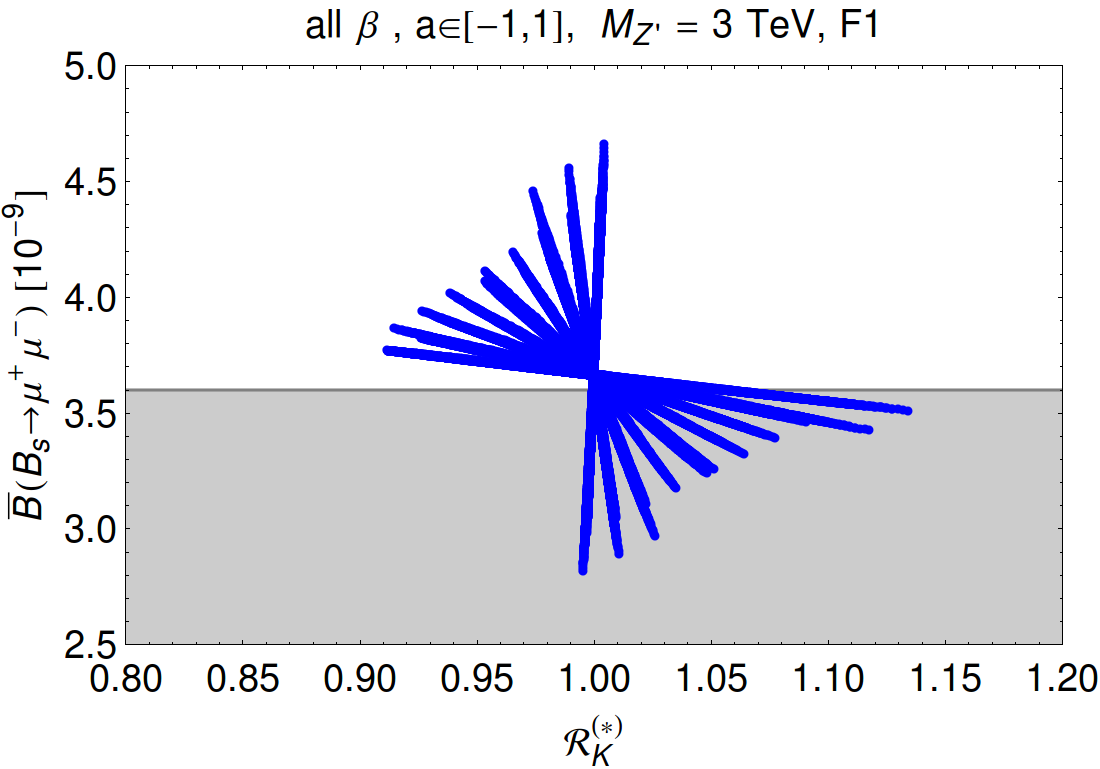
Refer to caption
Refer to caption
Figure 7: Correlation BR¯(Bsμ+μ)¯BRsubscript𝐵𝑠superscript𝜇superscript𝜇\overline{\text{BR}}(B_{s}\to\mu^{+}\mu^{-}) versus K()superscriptsubscript𝐾\mathcal{R}_{K}^{(*)} in the 331 model for MZ=3subscript𝑀superscript𝑍3M_{Z^{\prime}}=3\leavevmode\nobreak\ TeV for fermion representations F1 (left) and F2 (right).

In figure 7, we show the correlation between BR¯(Bsμ+μ)¯BRsubscript𝐵𝑠superscript𝜇superscript𝜇\overline{\text{BR}}(B_{s}\to\mu^{+}\mu^{-}) and K()superscriptsubscript𝐾\mathcal{R}_{K}^{(*)} for both fermion representations. In contrast to [24], where we considered in total 24 versions of the model, we study here an even larger set, since we do not fix the model parameter a𝑎a to three different values. Here we set MZ=3subscript𝑀superscript𝑍3M_{Z^{\prime}}=3\leavevmode\nobreak\ TeV, scanned over a[1,1]𝑎11a\in[-1,1] (corresponding to tanβ¯=[0,]¯𝛽0\tan\bar{\beta}=[0,\infty]) and over β=±2/3,±1/3𝛽plus-or-minus23plus-or-minus13\beta=\pm 2/\sqrt{3},\pm 1/\sqrt{3}. Constraints from bs+𝑏𝑠superscriptsuperscriptb\to s\ell^{+}\ell^{-} transitions (2σ2𝜎2\sigma range) and electroweak observables as in [24] (Ω33116superscriptΩ33116\Omega^{331}\leq 16) are included. One can see that even when combining all models a suppression of Bsμ+μsubscript𝐵𝑠superscript𝜇superscript𝜇B_{s}\to\mu^{+}\mu^{-}, as favoured by present data, almost always implies an enhancement of bsνν¯𝑏𝑠𝜈¯𝜈b\to s\nu\bar{\nu}. Models where both are enhanced or suppressed simultaneously are excluded due to electroweak observables constraints.

On the whole, 331 models are an example that specific NP models can be much more predictive than a generic EFT approach. The size of the NP effects in bsνν¯𝑏𝑠𝜈¯𝜈b\to s\nu\bar{\nu} in 331 models turn out to be small, typically below 15%percent1515\% at the level of the branching ratios.

4.3 Partial Compositeness

Partial quark compositeness is a feature of composite Higgs models and of the four-dimensional Kaluza-Klein picture of models with extra dimensions. Rare B𝐵B decays in a simple 4D partial compositeness model with different choices for the flavour structure and the representations of composite fermions have been considered in [22]. The dominant contributions to bsνν¯𝑏𝑠𝜈¯𝜈b\to s\nu\bar{\nu} transitions in these models come from tree-level flavour-changing Z𝑍Z couplings, i.e. contributions to the operators c~Zsubscript~𝑐𝑍\widetilde{c}_{Z} (in the “bidoublet model”) or c~Zsuperscriptsubscript~𝑐𝑍\widetilde{c}_{Z}^{\prime} (in the “triplet model”). Consequently, the bounds in (38) apply and limit the size of NP effects in BK()νν¯𝐵superscript𝐾𝜈¯𝜈B\to K^{(*)}\nu\bar{\nu}. The accessible range for Ksubscript𝐾\mathcal{R}_{K} and Ksubscriptsuperscript𝐾\mathcal{R}_{K^{*}} is shown in figure 8. The blue points correspond to the bidoublet model, the yellow points to the triplet model. The lighter points are disfavoured at 2σ2𝜎2\sigma by bsμ+μ𝑏𝑠superscript𝜇superscript𝜇b\to s\mu^{+}\mu^{-} data.

Refer to caption
Figure 8: Allowed ranges for the BKνν¯𝐵𝐾𝜈¯𝜈B\to K\nu\bar{\nu} and BKνν¯𝐵superscript𝐾𝜈¯𝜈B\to K^{*}\nu\bar{\nu} branching ratios in models with partial compositeness, normalized to the SM values, for two different choices of fermion representations: bidoublet model (blue), triplet model (yellow). Light points are disfavoured at 2σ2𝜎2\sigma by bsμ+μ𝑏𝑠superscript𝜇superscript𝜇b\to s\mu^{+}\mu^{-} data. Plot adapted from [22].

This can be compared to the Randall-Sundrum model with custodial protection (RSc) studied in [58, 25]. The fermion representations chosen in this model are similar to the triplet model of [22] and the NP effects in bνν¯𝑏𝜈¯𝜈b\to\nu\bar{\nu} are dominated by c~Zsuperscriptsubscript~𝑐𝑍\widetilde{c}_{Z}^{\prime}. However, since the extra dimensional model is much more restrictive, linking e.g. the scale of fermion resonances to that of the vector resonances, which are more strongly constrained experimentally, the maximal allowed effects in the RSc are significantly smaller. Larger effects were found in the Randall-Sundrum model without custodial protection [59], however in that case it is difficult to fulfill electroweak precision constraints, in particular from the T𝑇T parameter.

Effects in Wilson coefficients other than c~Zsubscript~𝑐𝑍\tilde{c}_{Z} and c~Zsuperscriptsubscript~𝑐𝑍\tilde{c}_{Z}^{\prime} could be generated in models with partial compositeness by heavy vector resonance exchange if any of the leptons has a sizable degree of compositeness for its left-handed chirality (the products of degrees of compositeness of both chiralities have to be small because of the leptons’ lightness). Depending on the representations of the composite fermions, one can then generate contributions to the Wilson coefficients (c~ql(1))superscriptsuperscriptsubscript~𝑐𝑞𝑙1(\tilde{c}_{ql}^{(1)})^{\ell\ell}, (c~ql(3))superscriptsuperscriptsubscript~𝑐𝑞𝑙3(\tilde{c}_{ql}^{(3)})^{\ell\ell}, and (c~dl)superscriptsubscript~𝑐𝑑𝑙(\tilde{c}_{dl})^{\ell\ell}, where =e,μ𝑒𝜇\ell=e,\mu, or τ𝜏\tau. Up to model-dependent (complex) O(1)𝑂1O(1) factors, the Wilson coefficients are parametrically given by

(c~ql(1,3))superscriptsuperscriptsubscript~𝑐𝑞𝑙13\displaystyle(\tilde{c}_{ql}^{(1,3)})^{\ell\ell} gρ2VtbVtssLbsLssL2[5TeVmρ]2,similar-toabsentsuperscriptsubscript𝑔𝜌2subscript𝑉𝑡𝑏superscriptsubscript𝑉𝑡𝑠subscript𝑠𝐿𝑏subscript𝑠𝐿𝑠superscriptsubscript𝑠𝐿2superscriptdelimited-[]5TeVsubscript𝑚𝜌2\displaystyle\sim\frac{g_{\rho}^{2}}{V_{tb}V_{ts}^{*}}s_{Lb}s_{Ls}s_{L\ell}^{2}\left[\frac{5\,\text{TeV}}{m_{\rho}}\right]^{2}\,, (c~dl)superscriptsubscript~𝑐𝑑𝑙\displaystyle(\tilde{c}_{dl})^{\ell\ell} gρ2VtbVtssRbsRssL2[5TeVmρ]2,similar-toabsentsuperscriptsubscript𝑔𝜌2subscript𝑉𝑡𝑏superscriptsubscript𝑉𝑡𝑠subscript𝑠𝑅𝑏subscript𝑠𝑅𝑠superscriptsubscript𝑠𝐿2superscriptdelimited-[]5TeVsubscript𝑚𝜌2\displaystyle\sim\frac{g_{\rho}^{2}}{V_{tb}V_{ts}^{*}}s_{Rb}s_{Rs}s_{L\ell}^{2}\left[\frac{5\,\text{TeV}}{m_{\rho}}\right]^{2}\,, (79)

where gρsubscript𝑔𝜌g_{\rho} and mρsubscript𝑚𝜌m_{\rho} are a typical coupling and mass scale of the vector resonances and sLf,Rfsubscript𝑠𝐿𝑓𝑅𝑓s_{Lf,Rf} is the degree of compositeness of the left-handed or right-handed fermion. As an example, we can consider models with flavour anarchy, where one expects sLbsLsVtbVts0.04similar-tosubscript𝑠𝐿𝑏subscript𝑠𝐿𝑠subscript𝑉𝑡𝑏superscriptsubscript𝑉𝑡𝑠similar-to0.04s_{Lb}s_{Ls}\sim V_{tb}V_{ts}^{*}\sim 0.04 and sRbsRsmdms/v2/(VtbVts)0.01similar-tosubscript𝑠𝑅𝑏subscript𝑠𝑅𝑠subscript𝑚𝑑subscript𝑚𝑠superscript𝑣2subscript𝑉𝑡𝑏superscriptsubscript𝑉𝑡𝑠similar-to0.01s_{Rb}s_{Rs}\sim m_{d}m_{s}/v^{2}/(V_{tb}V_{ts}^{*})\sim 0.01. For mρ/gρ1similar-tosubscript𝑚𝜌subscript𝑔𝜌1m_{\rho}/g_{\rho}\sim 1\,TeV, we see that, barring an additional enhancement, visible effects in the 4-fermion operators require an O(1)𝑂1O(1) degree of lepton compositeness. In general, one then also expects corrections to ZLL𝑍subscript𝐿subscript𝐿Z\ell_{L}\ell_{L} couplings of order sL2gρ2/mρ2superscriptsubscript𝑠𝐿2superscriptsubscript𝑔𝜌2superscriptsubscript𝑚𝜌2s_{L\ell}^{2}g_{\rho}^{2}/m_{\rho}^{2} that are excluded by LEP precision measurements at the Z𝑍Z pole for sLsubscript𝑠𝐿s_{L\ell} of O(1)𝑂1O(1). However, in models where the ZLL𝑍subscript𝐿subscript𝐿Z\ell_{L}\ell_{L} couplings are protected by a custodial symmetry (see e.g. [60]), such scenario could still be viable. An exhaustive analysis of this scenario is beyond the scope of our analysis.

4.4 MSSM

In the MSSM, the dominant NP effects in bsνν¯𝑏𝑠𝜈¯𝜈b\to s\nu\bar{\nu} arise from Z𝑍Z penguins, i.e. through c~Zsubscript~𝑐𝑍\widetilde{c}_{Z} and c~Zsuperscriptsubscript~𝑐𝑍\widetilde{c}_{Z}^{\prime}. While the former can be generated in the MSSM with MFV, the latter requires non-minimal flavour violation. However, it has been shown already in [17] that c~Zsuperscriptsubscript~𝑐𝑍\widetilde{c}_{Z}^{\prime} is very small throughout the MSSM parameter space once constraints from other flavour observables (notably Bsμ+μsubscript𝐵𝑠superscript𝜇superscript𝜇B_{s}\to\mu^{+}\mu^{-}) are taken into account and that sizable effects in c~Zsubscript~𝑐𝑍\widetilde{c}_{Z} are only possible beyond MFV, in particular in the presence of a flavour-changing trilinear coupling in the up-type squark sector.

In view of the improved constraints on both ΔF=1Δ𝐹1\Delta F=1 and ΔF=2Δ𝐹2\Delta F=2 observables in the bs𝑏𝑠b\to s sector as well as improved direct bounds on sparticle masses, we have performed a numerical analysis of the MSSM parameter space to asses the maximal size of NP effects in bsνν¯𝑏𝑠𝜈¯𝜈b\to s\nu\bar{\nu} still allowed in the MSSM. Our starting point is the 24-parameter phenomenological MSSM, to which we add all off-diagonal terms in the squark mass matrices and trilinear couplings relevant for bs𝑏𝑠b\to s transitions. The flavour diagonal parameters are scanned in the following ranges,

M1subscript𝑀1\displaystyle M_{1} [1,1500]GeV,absent11500GeV\displaystyle\in[1,1500]\,\text{GeV}, mQ~1,mU~1,mD~1subscript𝑚subscript~𝑄1subscript𝑚subscript~𝑈1subscript𝑚subscript~𝐷1\displaystyle m_{\tilde{Q}_{1}},m_{\tilde{U}_{1}},m_{\tilde{D}_{1}} [400,3000]GeV,absent4003000GeV\displaystyle\in[400,3000]\,\text{GeV}, (80)
M2subscript𝑀2\displaystyle M_{2} [100,1500]GeV,absent1001500GeV\displaystyle\in[100,1500]\,\text{GeV}, mQ~3,mU~3,mD~3subscript𝑚subscript~𝑄3subscript𝑚subscript~𝑈3subscript𝑚subscript~𝐷3\displaystyle m_{\tilde{Q}_{3}},m_{\tilde{U}_{3}},m_{\tilde{D}_{3}} [400,3000]GeV,absent4003000GeV\displaystyle\in[400,3000]\,\text{GeV}, (81)
M3subscript𝑀3\displaystyle M_{3} [400,3000]GeV,absent4003000GeV\displaystyle\in[400,3000]\,\text{GeV}, mL~1,mν~1subscript𝑚subscript~𝐿1subscript𝑚subscript~𝜈1\displaystyle m_{\tilde{L}_{1}},m_{\tilde{\nu}_{1}} [100,3000]GeV,absent1003000GeV\displaystyle\in[100,3000]\,\text{GeV}, (82)
|μ|𝜇\displaystyle|\mu| [100,1500]GeV,absent1001500GeV\displaystyle\in[100,1500]\,\text{GeV}, mL~3,mν~3subscript𝑚subscript~𝐿3subscript𝑚subscript~𝜈3\displaystyle m_{\tilde{L}_{3}},m_{\tilde{\nu}_{3}} [100,1500]GeV,absent1001500GeV\displaystyle\in[100,1500]\,\text{GeV}, (83)
MAsubscript𝑀𝐴\displaystyle M_{A} [100,1500]GeVabsent1001500GeV\displaystyle\in[100,1500]\,\text{GeV} Au,d,lsubscript𝐴𝑢𝑑𝑙\displaystyle A_{u,d,l} [3000,3000]GeV,absent30003000GeV\displaystyle\in[-3000,3000]\,\text{GeV}, (84)

where the trilinear parameters are scanned linearly and all others logarithmically. The gaugino masses and the μ𝜇\mu term are assumed to be real; both signs are allowed for μ𝜇\mu. We define the mass insertions as

(δLL)ijsubscriptsuperscript𝛿𝐿𝐿𝑖𝑗\displaystyle(\delta^{LL})_{ij} =(mQ2)ij(mQ2)ii(mQ2)jj,absentsubscriptsuperscriptsubscript𝑚𝑄2𝑖𝑗subscriptsuperscriptsubscript𝑚𝑄2𝑖𝑖subscriptsuperscriptsubscript𝑚𝑄2𝑗𝑗\displaystyle=\frac{(m_{Q}^{2})_{ij}}{\sqrt{(m_{Q}^{2})_{ii}(m_{Q}^{2})_{jj}}}\,, (δu,dRR)ijsubscriptsubscriptsuperscript𝛿𝑅𝑅𝑢𝑑𝑖𝑗\displaystyle(\delta^{RR}_{u,d})_{ij} =(mU,D2)ij(mU,D2)ii(mU,D2)jj,absentsubscriptsuperscriptsubscript𝑚𝑈𝐷2𝑖𝑗subscriptsuperscriptsubscript𝑚𝑈𝐷2𝑖𝑖subscriptsuperscriptsubscript𝑚𝑈𝐷2𝑗𝑗\displaystyle=\frac{(m_{U,D}^{2})_{ij}}{\sqrt{(m_{U,D}^{2})_{ii}(m_{U,D}^{2})_{jj}}}\,, (85)
(δu,dLR)ijsubscriptsubscriptsuperscript𝛿𝐿𝑅𝑢𝑑𝑖𝑗\displaystyle(\delta^{LR}_{u,d})_{ij} =(TU,D)ij(mQ2)ii(mU,D2)jj,absentsubscriptsubscript𝑇𝑈𝐷𝑖𝑗subscriptsuperscriptsubscript𝑚𝑄2𝑖𝑖subscriptsuperscriptsubscript𝑚𝑈𝐷2𝑗𝑗\displaystyle=\frac{(T_{U,D})_{ij}}{\sqrt{(m_{Q}^{2})_{ii}(m_{U,D}^{2})_{jj}}}\,, (86)

and scan |(δu,dLR)23,32|subscriptsubscriptsuperscript𝛿𝐿𝑅𝑢𝑑2332|(\delta^{LR}_{u,d})_{23,32}|, |(δu,dRR)23|subscriptsubscriptsuperscript𝛿𝑅𝑅𝑢𝑑23|(\delta^{RR}_{u,d})_{23}|, and |(δLL)23|subscriptsuperscript𝛿𝐿𝐿23|(\delta^{LL})_{23}| logarithmically between 104superscript10410^{-4} and 1, allowing for an arbitrary phase. Finally, we require the lightest neutralino to be the LSP and use FastLim 1.0 [61] to impose LHC bounds on sparticle masses and SUSY_FLAVOR 2.11 [62] to compute the bsνν¯𝑏𝑠𝜈¯𝜈b\to s\nu\bar{\nu} Wilson coefficients and impose FCNC constraints, in particular BR(BXsγ𝐵subscript𝑋𝑠𝛾B\to X_{s}\gamma), BR(Bsμ+μsubscript𝐵𝑠superscript𝜇superscript𝜇B_{s}\to\mu^{+}\mu^{-}), ΔMsΔsubscript𝑀𝑠\Delta M_{s}, and ϕssubscriptitalic-ϕ𝑠\phi_{s}.

Refer to caption
Figure 9: Allowed ranges for the BKνν¯𝐵𝐾𝜈¯𝜈B\to K\nu\bar{\nu} and BK()νν¯𝐵superscript𝐾𝜈¯𝜈B\to K^{(*)}\nu\bar{\nu} branching ratios in the MSSM, normalized to the SM values. All dark points pass flavour and collider constraints; black points have the corrected lightest Higgs mass.

The result of the parameter scan is shown in figure 9. All points shown are allowed by flavour constraints. Light gray points are ruled out by direct LHC bounds. Among the allowed points, we distinguish the black ones that have a lightest Higgs mass (computed with SPheno 3.3.2 [63, 64]) within 4 GeV of the true value of 125 GeV from the light blue ones, that have a too light or too heavy lightest Higgs. Our rationale for showing these points as well is that they might be realized in extensions of the MSSM raising the tree-level Higgs mass.

The numerical results confirm the findings of [17] that right-handed current contributions to bsνν¯𝑏𝑠𝜈¯𝜈b\to s\nu\bar{\nu} are small in the MSSM, so the relation K=Ksubscript𝐾subscriptsuperscript𝐾\mathcal{R}_{K}=\mathcal{R}_{K^{*}}, indicated by a dashed line in figure 9, is approximately fulfilled. The BKνν¯𝐵𝐾𝜈¯𝜈B\to K\nu\bar{\nu} and BK()νν¯𝐵superscript𝐾𝜈¯𝜈B\to K^{(*)}\nu\bar{\nu} can be enhanced or suppressed by at most 30% relative to the SM. This conclusion is not changed by the existing LHC direct bounds on sparticle masses, which have been taken into account in our scan as described above.

4.5 Leptoquarks

In models with leptoquarks one assumes the presence of heavy (scalar or vector) particles which carry colour and, thus, lead to interactions connecting leptons and quarks. This generically happens in GUTs or in SUSY theories with R-parity violation. As a consequence, the four-fermion operators (25) relevant for bsνν¯𝑏𝑠𝜈¯𝜈b\rightarrow s\nu\bar{\nu} and bs+𝑏𝑠superscriptsuperscriptb\rightarrow s\ell^{+}\ell^{-} processes can be generated by a tree-level exchange of the heavy leptoquark.

Spin GSMsubscript𝐺SMG_{\mathrm{SM}} interaction term generated Wilson coefficients
S1subscript𝑆1S_{1} 0 (𝟑¯,𝟏)13subscript¯3113\left(\overline{\mathbf{3}},\mathbf{1}\right)_{\frac{1}{3}} λij(qLic¯ϵlLj)ϕsubscript𝜆𝑖𝑗¯subscriptsuperscript𝑞𝑐𝐿𝑖italic-ϵsubscript𝑙𝐿𝑗italic-ϕ\lambda_{ij}\,\left(\overline{q^{c}_{{L}i}}\cdot\epsilon\cdot l_{{L}j}\right)\,\phi [cql(1)]ij;klΛ2=[cql(3)]ij;klΛ2=14λjlλikmϕ2subscriptdelimited-[]superscriptsubscript𝑐𝑞𝑙1𝑖𝑗𝑘𝑙superscriptΛ2subscriptdelimited-[]superscriptsubscript𝑐𝑞𝑙3𝑖𝑗𝑘𝑙superscriptΛ214subscript𝜆𝑗𝑙subscriptsuperscript𝜆𝑖𝑘superscriptsubscript𝑚italic-ϕ2\frac{\left[c_{ql}^{(1)}\right]_{ij;kl}}{\Lambda^{2}}=-\frac{\left[c_{ql}^{(3)}\right]_{ij;kl}}{\Lambda^{2}}=-\frac{1}{4}\frac{\lambda_{jl}\lambda^{*}_{ik}}{m_{\phi}^{2}}
S3subscript𝑆3S_{3} 0 (𝟑¯,𝟑)13subscript¯3313\left(\overline{\mathbf{3}},\mathbf{3}\right)_{\frac{1}{3}} λij(qLic¯ϵτalLj)ϕasubscript𝜆𝑖𝑗¯subscriptsuperscript𝑞𝑐𝐿𝑖italic-ϵsuperscript𝜏𝑎subscript𝑙𝐿𝑗superscriptitalic-ϕ𝑎\lambda_{ij}\,\left(\overline{q^{c}_{{L}i}}\cdot\epsilon\cdot\tau^{a}\cdot l_{{L}j}\right)\,\phi^{a} [cql(1)]ij;klΛ2=3[cql(3)]ij;klΛ2=34λjlλikmϕ2subscriptdelimited-[]superscriptsubscript𝑐𝑞𝑙1𝑖𝑗𝑘𝑙superscriptΛ23subscriptdelimited-[]superscriptsubscript𝑐𝑞𝑙3𝑖𝑗𝑘𝑙superscriptΛ234subscript𝜆𝑗𝑙subscriptsuperscript𝜆𝑖𝑘superscriptsubscript𝑚italic-ϕ2\frac{\left[c_{ql}^{(1)}\right]_{ij;kl}}{\Lambda^{2}}=3\frac{\left[c_{ql}^{(3)}\right]_{ij;kl}}{\Lambda^{2}}=\frac{3}{4}\frac{\lambda_{jl}\lambda^{*}_{ik}}{m_{\phi}^{2}}
R~2subscript~𝑅2\widetilde{R}_{2} 0 (𝟑,𝟐)16subscript3216\left(\mathbf{3},\mathbf{2}\right)_{\frac{1}{6}} λijdRi¯(lLjϵϕ)subscript𝜆𝑖𝑗¯subscript𝑑𝑅𝑖subscript𝑙𝐿𝑗italic-ϵitalic-ϕ\lambda_{ij}\,\overline{d_{{R}i}}\left(l_{{L}j}\cdot\epsilon\cdot\phi\right) [cdl]ij;klΛ2=12λilλjkmϕ2subscriptdelimited-[]subscript𝑐𝑑𝑙𝑖𝑗𝑘𝑙superscriptΛ212subscript𝜆𝑖𝑙subscriptsuperscript𝜆𝑗𝑘superscriptsubscript𝑚italic-ϕ2\frac{\left[c_{dl}\right]_{ij;kl}}{\Lambda^{2}}=-\frac{1}{2}\frac{\lambda_{il}\lambda^{*}_{jk}}{m_{\phi}^{2}}
U1subscript𝑈1U_{1} 1 (𝟑,𝟏)23subscript3123\left(\mathbf{3},\mathbf{1}\right)_{\frac{2}{3}} λij(qLi¯γμlLj)ϕμsubscript𝜆𝑖𝑗¯subscript𝑞𝐿𝑖superscript𝛾𝜇subscript𝑙𝐿𝑗subscriptitalic-ϕ𝜇\lambda_{ij}\,\left(\overline{q_{{L}i}}\,\gamma^{\mu}\,l_{{L}j}\right)\,\phi_{\mu} [cql(1)]ij;klΛ2=[cql(3)]ij;klΛ2=12λilλjkmϕ2subscriptdelimited-[]superscriptsubscript𝑐𝑞𝑙1𝑖𝑗𝑘𝑙superscriptΛ2subscriptdelimited-[]superscriptsubscript𝑐𝑞𝑙3𝑖𝑗𝑘𝑙superscriptΛ212subscript𝜆𝑖𝑙subscriptsuperscript𝜆𝑗𝑘superscriptsubscript𝑚italic-ϕ2\frac{\left[c_{ql}^{(1)}\right]_{ij;kl}}{\Lambda^{2}}=\frac{\left[c_{ql}^{(3)}\right]_{ij;kl}}{\Lambda^{2}}=\frac{1}{2}\frac{\lambda_{il}\lambda^{*}_{jk}}{m_{\phi}^{2}}
U3subscript𝑈3U_{3} 1 (𝟑,𝟑)23subscript3323\left(\mathbf{3},\mathbf{3}\right)_{\frac{2}{3}} λij(qLi¯γμτalLj)ϕμasubscript𝜆𝑖𝑗¯subscript𝑞𝐿𝑖superscript𝛾𝜇superscript𝜏𝑎subscript𝑙𝐿𝑗subscriptsuperscriptitalic-ϕ𝑎𝜇\lambda_{ij}\,\left(\overline{q_{{L}i}}\,\gamma^{\mu}\,\tau^{a}\,l_{{L}j}\right)\,\phi^{a}_{\mu} [cql(1)]ij;klΛ2=3[cql(3)]ij;klΛ2=32λilλjkmϕ2subscriptdelimited-[]superscriptsubscript𝑐𝑞𝑙1𝑖𝑗𝑘𝑙superscriptΛ23subscriptdelimited-[]superscriptsubscript𝑐𝑞𝑙3𝑖𝑗𝑘𝑙superscriptΛ232subscript𝜆𝑖𝑙subscriptsuperscript𝜆𝑗𝑘superscriptsubscript𝑚italic-ϕ2\frac{\left[c_{ql}^{(1)}\right]_{ij;kl}}{\Lambda^{2}}=-3\frac{\left[c_{ql}^{(3)}\right]_{ij;kl}}{\Lambda^{2}}=-\frac{3}{2}\frac{\lambda_{il}\lambda^{*}_{jk}}{m_{\phi}^{2}}
V2subscript𝑉2V_{2} 1 (𝟑¯,𝟐)56subscript¯3256\left(\overline{\mathbf{3}},\mathbf{2}\right)_{\frac{5}{6}} λijdRic¯γμ(lLjϵϕμ)subscript𝜆𝑖𝑗¯superscriptsubscript𝑑𝑅𝑖𝑐superscript𝛾𝜇subscript𝑙𝐿𝑗italic-ϵsubscriptitalic-ϕ𝜇\lambda_{ij}\,\overline{d_{{R}i}^{c}}\,\gamma^{\mu}\left(l_{{L}j}\cdot\epsilon\cdot\phi_{\mu}\right) [cdl]ij;klΛ2=λilλjkmϕ2subscriptdelimited-[]subscript𝑐𝑑𝑙𝑖𝑗𝑘𝑙superscriptΛ2subscript𝜆𝑖𝑙subscriptsuperscript𝜆𝑗𝑘superscriptsubscript𝑚italic-ϕ2\frac{\left[c_{dl}\right]_{ij;kl}}{\Lambda^{2}}=\frac{\lambda_{il}\lambda^{*}_{jk}}{m_{\phi}^{2}}
Table 3: Possible leptoquark scenarios relevant for bsνν¯𝑏𝑠𝜈¯𝜈b\rightarrow s\nu\bar{\nu} decays. In the first columns, the spin and gauge quantum numbers are given as well as the relevant interaction term. In the last column, we give expressions for the Wilson coefficients of the generated four-fermion operators. The SM left-handed quark and lepton doublets are denoted by QLsubscript𝑄𝐿Q_{L} and LLsubscript𝐿𝐿L_{L}, respectively, while the leptoquark is written as ϕ(μ)subscriptitalic-ϕ𝜇\phi_{(\mu)}. We explicitly showed the flavour indices here.

The number of leptoquark models is strongly restricted by the assumption of SM gauge invariance. An extensive investigation of the viable scenarios is given in [65]. However, not all possible scenarios lead to bsνν¯𝑏𝑠𝜈¯𝜈b\rightarrow s\nu\bar{\nu} transitions. We summarize the viable options in Table 3 and give expressions for the Wilson coefficients of the generated operators. Generally, these models are not lepton flavour universal and even flavour violating. For the time being we assume that the leptoquarks only couple to one lepton flavour.

We find that the Wilson coefficients are strongly correlated. In models in which the leptoquark is an SU(2)SU2\mathrm{SU}(2) singlet or triplet only the operators Qql(1)superscriptsubscript𝑄𝑞𝑙1Q_{ql}^{(1)} and Qql(3)superscriptsubscript𝑄𝑞𝑙3Q_{ql}^{(3)} are generated, but predicted to obey the relation

c~ql(1)=nc~ql(3),superscriptsubscript~𝑐𝑞𝑙1𝑛superscriptsubscript~𝑐𝑞𝑙3\tilde{c}_{ql}^{(1)}=n\cdot\tilde{c}_{ql}^{(3)}, (87)

where n𝑛n is some model-dependent real constant. From (30)–(32) we then find that, for a given n𝑛n, the low-energy Wilson coefficients only depend on one parameter,

CLNPsuperscriptsubscript𝐶𝐿NP\displaystyle C_{L}^{\mathrm{NP}} =c~ql(1)c~ql(3)=(n1)c~ql(3),absentsuperscriptsubscript~𝑐𝑞𝑙1superscriptsubscript~𝑐𝑞𝑙3𝑛1superscriptsubscript~𝑐𝑞𝑙3\displaystyle=\tilde{c}_{ql}^{(1)}-\tilde{c}_{ql}^{(3)}=(n-1)\tilde{c}_{ql}^{(3)}, (88)
C9NP=C10NPsuperscriptsubscript𝐶9NPsuperscriptsubscript𝐶10NP\displaystyle C_{9}^{\mathrm{NP}}=-C_{10}^{\mathrm{NP}} =c~ql(1)+c~ql(3)=(n+1)c~ql(3),absentsuperscriptsubscript~𝑐𝑞𝑙1superscriptsubscript~𝑐𝑞𝑙3𝑛1superscriptsubscript~𝑐𝑞𝑙3\displaystyle=\tilde{c}_{ql}^{(1)}+\tilde{c}_{ql}^{(3)}=(n+1)\tilde{c}_{ql}^{(3)}, (89)
CR=C9=C10subscript𝐶𝑅superscriptsubscript𝐶9superscriptsubscript𝐶10\displaystyle C_{R}=C_{9}^{\prime}=C_{10}^{\prime} =0.absent0\displaystyle=0. (90)

Hence, we can write the corrections to the bsνν¯𝑏𝑠𝜈¯𝜈b\rightarrow s\nu\bar{\nu} branching ratios in the following way,

FL=1,K=K=23+13|CLSM+(n1)[c~ql(3)]|2|CLSM|2.formulae-sequencesubscriptsubscript𝐹𝐿1subscript𝐾subscriptsuperscript𝐾2313superscriptsuperscriptsubscript𝐶𝐿SM𝑛1subscriptdelimited-[]superscriptsubscript~𝑐𝑞𝑙32superscriptsuperscriptsubscript𝐶𝐿SM2\mathcal{R}_{F_{L}}=1,\qquad\mathcal{R}_{K}=\mathcal{R}_{K^{*}}=\frac{2}{3}+\frac{1}{3}\frac{\left|C_{L}^{\mathrm{SM}}+(n-1)\left[\tilde{c}_{ql}^{(3)}\right]_{\ell}\right|^{2}}{\left|C_{L}^{\mathrm{SM}}\right|^{2}}. (91)

In the case of a doublet leptoquark, only Qdlsubscript𝑄𝑑𝑙Q_{dl} is present. So again, we expect only a dependence on one parameter,

CLNP=C9NP=C10NPsuperscriptsubscript𝐶𝐿NPsuperscriptsubscript𝐶9NPsuperscriptsubscript𝐶10NP\displaystyle C_{L}^{\mathrm{NP}}=C_{9}^{\mathrm{NP}}=C_{10}^{\mathrm{NP}} =0,absent0\displaystyle=0, (92)
CR=C9=C10subscript𝐶𝑅superscriptsubscript𝐶9superscriptsubscript𝐶10\displaystyle C_{R}=C_{9}^{\prime}=-C_{10}^{\prime} =c~dl.absentsubscript~𝑐𝑑𝑙\displaystyle=\tilde{c}_{dl}. (93)

In this case, we find a contribution to η0𝜂0\eta\neq 0 such that also KKsubscript𝐾subscriptsuperscript𝐾\mathcal{R}_{K}\neq\mathcal{R}_{K^{*}},

Ksubscript𝐾\displaystyle\mathcal{R}_{K} =23+13(1+2CLSMRe([c~dl])|CLSM|2+|[c~dl]|2)(1+|[c~dl]|2|CLSM|2),absent231312superscriptsubscript𝐶𝐿SMResubscriptdelimited-[]subscript~𝑐𝑑𝑙superscriptsuperscriptsubscript𝐶𝐿SM2superscriptsubscriptdelimited-[]subscript~𝑐𝑑𝑙21superscriptsubscriptdelimited-[]subscript~𝑐𝑑𝑙2superscriptsuperscriptsubscript𝐶𝐿SM2\displaystyle=\frac{2}{3}+\frac{1}{3}\left(1+2\frac{C_{L}^{\mathrm{SM}}\,\mathrm{Re}\left(\left[\tilde{c}_{dl}\right]_{\ell}\right)}{|C_{L}^{\mathrm{SM}}|^{2}+|\left[\tilde{c}_{dl}\right]_{\ell}|^{2}}\right)\left(1+\frac{\left|\left[\tilde{c}_{dl}\right]_{\ell}\right|^{2}}{\left|C_{L}^{\mathrm{SM}}\right|^{2}}\right), (94)
Ksubscriptsuperscript𝐾\displaystyle\mathcal{R}_{K^{*}} =23+13(1κηCLSMRe([c~dl])|CLSM|2+|[c~dl]|2)(1+|[c~dl]|2|CLSM|2).absent23131subscript𝜅𝜂superscriptsubscript𝐶𝐿SMResubscriptdelimited-[]subscript~𝑐𝑑𝑙superscriptsuperscriptsubscript𝐶𝐿SM2superscriptsubscriptdelimited-[]subscript~𝑐𝑑𝑙21superscriptsubscriptdelimited-[]subscript~𝑐𝑑𝑙2superscriptsuperscriptsubscript𝐶𝐿SM2\displaystyle=\frac{2}{3}+\frac{1}{3}\left(1-\kappa_{\eta}\frac{C_{L}^{\mathrm{SM}}\,\mathrm{Re}\left(\left[\tilde{c}_{dl}\right]_{\ell}\right)}{|C_{L}^{\mathrm{SM}}|^{2}+|\left[\tilde{c}_{dl}\right]_{\ell}|^{2}}\right)\left(1+\frac{\left|\left[\tilde{c}_{dl}\right]_{\ell}\right|^{2}}{\left|C_{L}^{\mathrm{SM}}\right|^{2}}\right). (95)

From table 3, we can already see two special cases. In scenario U1subscript𝑈1U_{1} there is n=1𝑛1n=1 which implies that all contributions to K=Ksubscript𝐾subscriptsuperscript𝐾\mathcal{R}_{K}=\mathcal{R}_{K^{*}} vanish such that we do not expect any deviation from the SM values in this model. In the scenario S1subscript𝑆1S_{1}, on the other hand, we find n=1𝑛1n=-1, which means that this scenario does not give any contribution to the decay into charged leptons. Hence, the effects in Ksubscript𝐾\mathcal{R}_{K} and Ksubscriptsuperscript𝐾\mathcal{R}_{K^{*}} are unconstrained from these decays.

We can use the results of section 3 to set constraints on the different leptoquark scenarios. This very much depends on the lepton generation the leptoquark couples to.
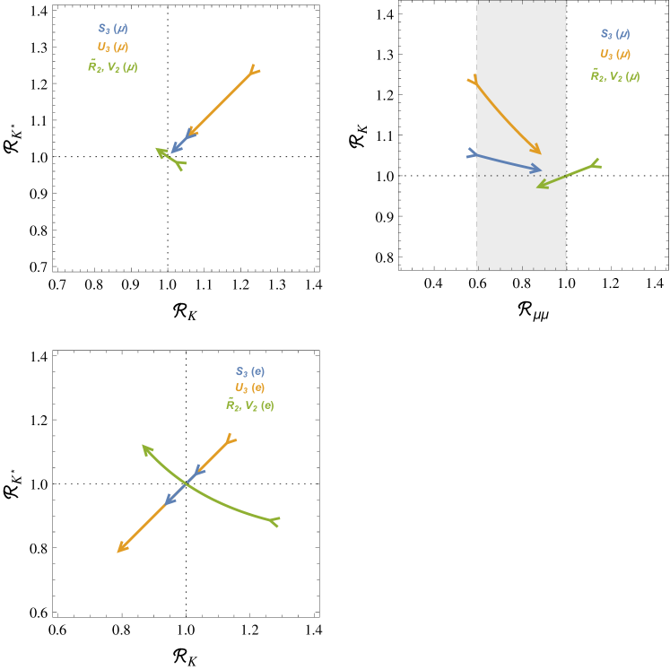
Refer to caption
Figure 10: Correlation between the branching fractions BKνν¯𝐵𝐾𝜈¯𝜈B\rightarrow K\nu\bar{\nu}, BKνν¯𝐵superscript𝐾𝜈¯𝜈B\rightarrow K^{*}\nu\bar{\nu} and Bsμμsubscript𝐵𝑠𝜇𝜇B_{s}\rightarrow\mu\mu for the different leptoquark models. We did not show the scenarios S1subscript𝑆1S_{1} and U1subscript𝑈1U_{1}, since in the first case K=Ksubscript𝐾subscriptsuperscript𝐾\mathcal{R}_{K}=\mathcal{R}_{K^{*}} is in principle unbounded and in the second case we do not expect a deviation from the SM value. First line: Only couplings to second generation leptons are allowed. Second line: Only couplings to first generation leptons are allowed.
=𝝁bold-ℓ𝝁\ell=\mu

If we assume that the leptoquarks only couple to second generation leptons, all the bounds from bsμ+μ𝑏𝑠superscript𝜇superscript𝜇b\rightarrow s\mu^{+}\mu^{-} decays apply, but they have to be rescaled by an appropriate factor depending on n𝑛n. A slight complication arises for the scenario V2subscript𝑉2V_{2}, since for this case the quantum numbers of the leptoquark also allow for a second interaction term, such that additionally the operator Qqesubscript𝑄𝑞𝑒Q_{qe} is generated. This operator then carries completely independent Wilson coefficients, which do not contribute to the decay into neutrinos but potentially affect the bounds from the decay into charged leptons. Fortunately, this additional operator only contributes to the unprimed operators C9subscript𝐶9C_{9} and C10subscript𝐶10C_{10} such that the bounds on c~dlsubscript~𝑐𝑑𝑙\tilde{c}_{dl} and c~qesubscript~𝑐𝑞𝑒\tilde{c}_{qe} are only weakly correlated. So, bounds from section 3 are only weakly modified.

The allowed values for the branching ratios are shown in figure 10.

=𝒆bold-ℓ𝒆\ell=e

If the leptoquarks only couple to first generation leptons then the bounds from section 3 apply. These are significantly weaker than for the case =μ𝜇\ell=\mu. The resulting bounds on the branching ratios are also shown in figure 10.

=𝝉bold-ℓ𝝉\ell=\tau

As already mentioned in section 3, the bounds on the decays into taus are very weak. This means that effectively there are no bounds for this case.

Until now, we assumed that the leptoquarks only couple to one generation of leptons. If we loosen this assumption we immediately get LFV. For the case of a coupling to third generation leptons we cannot find reasonable bounds due to the weak constraints from LFV processes involving taus. Thus, we only consider the case of non-vanishing couplings to the first two generations of leptons. For this we find that the following pattern of operators is generated schematically,

Csb;ee[Q]sb;ee+Csb;μμ[Q]sb;μμ+Csb;eμ[Q]sb;eμ+Csb;μe[Q]sb;μe+h.c.,formulae-sequencesubscript𝐶𝑠𝑏𝑒𝑒subscriptdelimited-[]𝑄𝑠𝑏𝑒𝑒subscript𝐶𝑠𝑏𝜇𝜇subscriptdelimited-[]𝑄𝑠𝑏𝜇𝜇subscript𝐶𝑠𝑏𝑒𝜇subscriptdelimited-[]𝑄𝑠𝑏𝑒𝜇subscript𝐶𝑠𝑏𝜇𝑒subscriptdelimited-[]𝑄𝑠𝑏𝜇𝑒hc\mathcal{L}\supset C_{sb;ee}\left[Q\right]_{sb;ee}+C_{sb;\mu\mu}\left[Q\right]_{sb;\mu\mu}+C_{sb;e\mu}\left[Q\right]_{sb;e\mu}+C_{sb;\mu e}\left[Q\right]_{sb;\mu e}\,\,+\,\,\mathrm{h.c.}, (96)

where the Wilson coefficients obey the relation

Csb;eeCsb;μμ=Csb;eμCsb;μe.subscript𝐶𝑠𝑏𝑒𝑒subscript𝐶𝑠𝑏𝜇𝜇subscript𝐶𝑠𝑏𝑒𝜇subscript𝐶𝑠𝑏𝜇𝑒C_{sb;ee}C_{sb;\mu\mu}=C_{sb;e\mu}C_{sb;\mu e}. (97)

We see that we can use the constraints on the flavour conserving Wilson coefficients to put constraints on the flavour violating ones, which are only weakly bounded. Except for some fine-tuned corners of parameter space, we find that one cannot expect large effects in the flavour-violating Wilson coefficients, implying that charged LFV decays like Bse±μsubscript𝐵𝑠superscript𝑒plus-or-minussuperscript𝜇minus-or-plusB_{s}\to e^{\pm}\mu^{\mp} are unlikely to be observable and that the contribution of the bsνeν¯μ𝑏𝑠subscript𝜈𝑒subscript¯𝜈𝜇b\to s\nu_{e}\bar{\nu}_{\mu} transition to the BK()νν¯𝐵superscript𝐾𝜈¯𝜈B\to K^{(*)}\nu\bar{\nu} signal should be small.

Summarizing the results on leptoquarks, we can say that in the case of coupling to muons (and muon neutrinos), the effects in K()subscriptsuperscript𝐾\mathcal{R}_{K^{(*)}} can at most be of the order of 25% for left-handed and 5% for right-handed quarks. For couplings to electrons (and electron neutrinos), also right-handed currents can lead to deviations at the level of 20% from the SM.

The exception to this is the scenario S1subscript𝑆1S_{1} where the effects can in principle be very large, since this model is not constrained by bs+𝑏𝑠superscriptsuperscriptb\rightarrow s\ell^{+}\ell^{-} data at all. In all leptoquark models, if the leptoquark only couples to taus (and tau neutrinos), the effects in K()subscriptsuperscript𝐾\mathcal{R}_{K^{(*)}} can be very large as well.

5 Summary and conclusions

In this paper, we have taken a close look at bsνν¯𝑏𝑠𝜈¯𝜈b\to s\nu\bar{\nu} transitions, in view of the reduced form factor uncertainties, calculation of complete NLO electroweak corrections and new constraints from other decays, in particular bsμ+μ𝑏𝑠superscript𝜇superscript𝜇b\to s\mu^{+}\mu^{-} transitions. In addition to presenting improved SM predictions, we have analyzed these decays in an effective field theory approach and in a number of explicit NP models. The numerous plots that exhibit the correlations between various observables demonstrate that these decays constitute a useful tool in constraining these models.
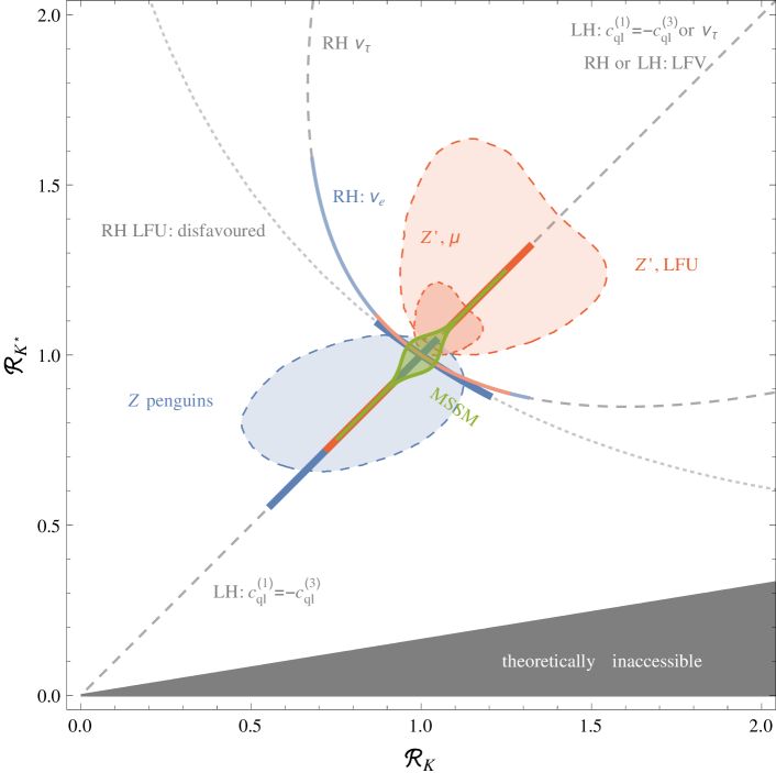
Refer to caption
Figure 11: Summary of allowed effects in the plane of BKνν¯𝐵𝐾𝜈¯𝜈B\to K\nu\bar{\nu} vs. BKνν¯𝐵superscript𝐾𝜈¯𝜈B\to K^{*}\nu\bar{\nu} normalized to their SM values for various NP scenarios. For details see text.

Of particular interest is the correlation between Ksubscript𝐾\mathcal{R}_{K} and Ksuperscriptsubscript𝐾\mathcal{R}_{K}^{*}. In figure 11, we collect the results for this correlation as obtained in several models:

  • The gray dashed line with K=Ksubscript𝐾superscriptsubscript𝐾\mathcal{R}_{K}=\mathcal{R}_{K}^{*} is the MFV relation. The violation of this relation in future data would signal non-MFV interactions and in particular right-handed currents at work. Staying on this line, there are three ways to obtain large deviations from the SM while avoiding bs+𝑏𝑠superscriptsuperscriptb\to s\ell^{+}\ell^{-} constraints:

    • Models generating the Wilson coefficients c~ql(1)=c~ql(3)superscriptsubscript~𝑐𝑞𝑙1superscriptsubscript~𝑐𝑞𝑙3\tilde{c}_{ql}^{(1)}=-\tilde{c}_{ql}^{(3)}, e.g. the leptoquark model S1subscript𝑆1S_{1} discussed in section 4.5, can in principle lead to arbitrarily small or large effects;

    • Models contributing only to operators with tau leptons and tau neutrinos can arbitrarily enhance the branching ratios, but there is a lower bound, K=K>2/3subscript𝐾superscriptsubscript𝐾23\mathcal{R}_{K}=\mathcal{R}_{K}^{*}>2/3;

    • Models contributing only to lepton flavour violating operators can only enhance the branching ratios. Interestingly, if NP only contributes to one LFV operator, the relation K=K>1subscript𝐾superscriptsubscript𝐾1\mathcal{R}_{K}=\mathcal{R}_{K}^{*}>1 holds for left- and right-handed operators.

  • The gray dashed line labeled “RH ντsubscript𝜈𝜏\nu_{\tau}” is accessible in models contributing only to (c~dl)ττsuperscriptsubscript~𝑐𝑑𝑙𝜏𝜏(\tilde{c}_{dl})^{\tau\tau}, i.e. right-handed currents with taus or tau neutrinos.

  • The gray dotted line corresponds to models with right-handed currents only and with LFU. However, in the case of LFU, the bs+𝑏𝑠superscriptsuperscriptb\to s\ell^{+}\ell^{-} bounds apply, so large deviations from the SM are disfavoured.

  • The coloured dark blue and red lines correspond to allowed effects when a single operator in the SM-EFT is varied. For details, see figure 1.

  • The light blue and red lines correspond to right-handed operators with electrons only. For details, see figure 4.

  • The blue area corresponds to simultaneous effects in left- and right-handed Z𝑍Z penguins (see figure 3).

  • The large red area corresponds to simultaneous effects in c~ql(1)superscriptsubscript~𝑐𝑞𝑙1\tilde{c}_{ql}^{(1)}, c~dlsubscript~𝑐𝑑𝑙\tilde{c}_{dl}, c~qesubscript~𝑐𝑞𝑒\tilde{c}_{qe}, and c~desubscript~𝑐𝑑𝑒\tilde{c}_{de} (see figure 3), assuming LFU, as happens in the presence of a single SU(2)L𝑆𝑈subscript2𝐿SU(2)_{L} singlet Zsuperscript𝑍Z^{\prime} gauge boson dominating the scene (cf. sec. 4.1).

  • The small red area corresponds to the same operators as above, but assuming NP contributions only to operators with muons or muon neutrinos.

  • The green area corresponds to the MSSM (see figure 9).


The main messages from this analysis are as follows:

  • The uncertainties in SM predictions for the branching ratios for BK()νν¯𝐵superscript𝐾𝜈¯𝜈B\to K^{(*)}\nu\bar{\nu} have been reduced down to 10%percent1010\%.

  • The SM branching ratio for BKνν¯𝐵superscript𝐾𝜈¯𝜈B\to K^{*}\nu\bar{\nu} is found to be by 40%percent4040\% larger than previous estimates which could allow to observe this decay earlier than expected until now if we assume that NP contributions do not significantly suppress its rate.

  • The precise measurements of decays based on the bsμ+μ𝑏𝑠superscript𝜇superscript𝜇b\to s\mu^{+}\mu^{-} transition can be used to put constraints on the size of effects in the BK()νν¯𝐵superscript𝐾𝜈¯𝜈B\to K^{(*)}\nu\bar{\nu} decays, barring cancellations. Assuming LFU, this limits the relative deviations from the SM to roughly ±60%plus-or-minuspercent60\pm 60\%. If NP is assumed to affect only muons (and muon neutrinos), the effects are at most ±20%plus-or-minuspercent20\pm 20\%.

  • We have emphasized that bsνν¯𝑏𝑠𝜈¯𝜈b\to s\nu\bar{\nu} transitions could help to disentangle possible NP dynamics behind the anomalies presently observed in BK()μ+μ𝐵superscript𝐾superscript𝜇superscript𝜇B\to K^{(*)}\mu^{+}\mu^{-} decays. This is seen in several plots presented by us, in particular in figures 1 and 3.

  • In the presence of flavour non-universality in the lepton couplings, NP effects in bsνν¯𝑏𝑠𝜈¯𝜈b\to s\nu\bar{\nu} could be large, in particular if NP only couples to taus (and tau neutrinos). In fact, the BK()νν¯𝐵superscript𝐾𝜈¯𝜈B\to K^{(*)}\nu\bar{\nu} decays can be used to put indirect bounds on bsτ+τ𝑏𝑠superscript𝜏superscript𝜏b\to s\tau^{+}\tau^{-} transitions. Some of the leptoquark models discussed by us represent concrete realizations of such a NP scenario. This shows that, without any dynamical assumptions, finding small NP effects in bsμ+μ𝑏𝑠superscript𝜇superscript𝜇b\to s\mu^{+}\mu^{-} transitions would not necessarily imply that in bsνν¯𝑏𝑠𝜈¯𝜈b\to s\nu\bar{\nu} transitions these effects should also be small.

  • In several NP scenarios, like the MSSM, 331 models, models with partial compositeness and models with MFV, NP contributions to the branching ratios are not found larger than 30%percent3030\% relative to their SM values.

In summary, our analysis demonstrates that the simultaneous study of the decays BK()νν¯𝐵superscript𝐾𝜈¯𝜈B\to K^{(*)}\nu\bar{\nu}, BK()μ+μ𝐵superscript𝐾superscript𝜇superscript𝜇B\to K^{(*)}\mu^{+}\mu^{-}, and Bsμ+μsubscript𝐵𝑠superscript𝜇superscript𝜇B_{s}\to\mu^{+}\mu^{-} in the coming years will teach us a lot about the structure of possible new dynamics at the short distance scales in the reach of the LHC and even at much short distance scales. The measurement of the rate for K+π+νν¯superscript𝐾superscript𝜋𝜈¯𝜈K^{+}\to\pi^{+}\nu\bar{\nu} by NA62 in the coming years should also contribute in an important manner to these studies, possibly signalling the presence of non-MFV interactions.

Acknowledgments

It is a pleasure to thank Wolfgang Altmannshofer for useful discussions. We are indebted to Aoife Bharucha and Roman Zwicky for sharing preliminary results on BK𝐵superscript𝐾B\to K^{*} form factors. The research of A.B. and J.G.-N. was done and financed in the context of the ERC Advanced Grant project “FLAVOUR” (267104). C.N. and D.S. were supported by the DFG cluster of excellence “Origin and Structure of the Universe”.

Appendix A Form factors

For the BK𝐵superscript𝐾B\to K^{*} form factors, we use the combined fit to lattice and LCSR results recently performed in [32]. The ρ𝜌\rho and κ𝜅\kappa parameters used in section 2 are defined in terms of BK𝐵superscript𝐾B\to K^{*} form factors as

ρV(q2)subscript𝜌𝑉superscript𝑞2\displaystyle\rho_{V}(q^{2}) =2q2λK3/2(q2)(mB+mK)2mB4[V(q2)]2,absent2superscript𝑞2subscriptsuperscript𝜆32superscript𝐾superscript𝑞2superscriptsubscript𝑚𝐵subscript𝑚superscript𝐾2superscriptsubscript𝑚𝐵4superscriptdelimited-[]𝑉superscript𝑞22\displaystyle=\frac{2q^{2}\lambda^{3/2}_{K^{*}}(q^{2})}{(m_{B}+{m}_{K^{*}})^{2}m_{B}^{4}}\left[V(q^{2})\right]^{2}\,, (98)
ρA1(q2)subscript𝜌subscript𝐴1superscript𝑞2\displaystyle\rho_{A_{1}}(q^{2}) =2q2λK1/2(q2)(mB+mK)2mB4[A1(q2)]2,absent2superscript𝑞2subscriptsuperscript𝜆12superscript𝐾superscript𝑞2superscriptsubscript𝑚𝐵subscript𝑚superscript𝐾2superscriptsubscript𝑚𝐵4superscriptdelimited-[]subscript𝐴1superscript𝑞22\displaystyle=\frac{2q^{2}\lambda^{1/2}_{K^{*}}(q^{2})(m_{B}+{m}_{K^{*}})^{2}}{m_{B}^{4}}\left[A_{1}(q^{2})\right]^{2}\,, (99)
ρA12(q2)subscript𝜌subscript𝐴12superscript𝑞2\displaystyle\rho_{A_{12}}(q^{2}) =64mK2λK1/2(q2)mB2[A12(q2)]2,absent64superscriptsubscript𝑚superscript𝐾2subscriptsuperscript𝜆12superscript𝐾superscript𝑞2superscriptsubscript𝑚𝐵2superscriptdelimited-[]subscript𝐴12superscript𝑞22\displaystyle=\frac{64{m}_{K^{*}}^{2}\lambda^{1/2}_{K^{*}}(q^{2})}{m_{B}^{2}}\left[A_{12}(q^{2})\right]^{2}\,, (100)
κη(q2)subscript𝜅𝜂superscript𝑞2\displaystyle\kappa_{\eta}(q^{2}) =2ρA1(q2)+ρA12(q2)ρV(q2)ρA1(q2)+ρA12(q2)+ρV(q2),absent2subscript𝜌subscript𝐴1superscript𝑞2subscript𝜌subscript𝐴12superscript𝑞2subscript𝜌𝑉superscript𝑞2subscript𝜌subscript𝐴1superscript𝑞2subscript𝜌subscript𝐴12superscript𝑞2subscript𝜌𝑉superscript𝑞2\displaystyle=2\,\frac{\rho_{A_{1}}(q^{2})+\rho_{A_{12}}(q^{2})-\rho_{V}(q^{2})}{\rho_{A_{1}}(q^{2})+\rho_{A_{12}}(q^{2})+\rho_{V}(q^{2})}\,, (101)

where

λ(a,b,c)𝜆𝑎𝑏𝑐\displaystyle\lambda(a,b,c) =a2+b2+c22(ab+bc+ac),absentsuperscript𝑎2superscript𝑏2superscript𝑐22𝑎𝑏𝑏𝑐𝑎𝑐\displaystyle=a^{2}+b^{2}+c^{2}-2(ab+bc+ac)\,, λK()(q2)λ(mB2,mK()2,q2).subscript𝜆superscript𝐾superscript𝑞2𝜆superscriptsubscript𝑚𝐵2superscriptsubscript𝑚superscript𝐾2superscript𝑞2\displaystyle\lambda_{K^{(*)}}(q^{2})\equiv\lambda(m_{B}^{2},m_{K^{(*)}}^{2},q^{2})\,. (102)

In the case of binned observables, the correct definition of κηsubscript𝜅𝜂\kappa_{\eta} to be used reads

κη|[a,b]evaluated-atsubscript𝜅𝜂𝑎𝑏\displaystyle\kappa_{\eta}|_{[a,b]} =2ab𝑑q2(ρA1(q2)+ρA12(q2)ρV(q2))ab𝑑q2(ρA1(q2)+ρA12(q2)+ρV(q2)).absent2superscriptsubscript𝑎𝑏differential-dsuperscript𝑞2subscript𝜌subscript𝐴1superscript𝑞2subscript𝜌subscript𝐴12superscript𝑞2subscript𝜌𝑉superscript𝑞2superscriptsubscript𝑎𝑏differential-dsuperscript𝑞2subscript𝜌subscript𝐴1superscript𝑞2subscript𝜌subscript𝐴12superscript𝑞2subscript𝜌𝑉superscript𝑞2\displaystyle=2\,\frac{\int_{a}^{b}dq^{2}\leavevmode\nobreak\ (\rho_{A_{1}}(q^{2})+\rho_{A_{12}}(q^{2})-\rho_{V}(q^{2}))}{\int_{a}^{b}dq^{2}\leavevmode\nobreak\ (\rho_{A_{1}}(q^{2})+\rho_{A_{12}}(q^{2})+\rho_{V}(q^{2}))}\,. (103)

For the BK𝐵𝐾B\to K form factors, we proceed in a similar way. We consider the z𝑧z expansion of the form factor f+subscript𝑓f_{+},

f+(q2)=11q2/m+2[α0+α1z(q2)+α2z2(q2)+z3(q2)3(α1+2α2)],subscript𝑓superscript𝑞211superscript𝑞2superscriptsubscript𝑚2delimited-[]subscript𝛼0subscript𝛼1𝑧superscript𝑞2subscript𝛼2superscript𝑧2superscript𝑞2superscript𝑧3superscript𝑞23subscript𝛼12subscript𝛼2f_{+}(q^{2})=\frac{1}{1-q^{2}/m_{+}^{2}}\left[\alpha_{0}+\alpha_{1}z(q^{2})+\alpha_{2}z^{2}(q^{2})+\frac{z^{3}(q^{2})}{3}(-\alpha_{1}+2\alpha_{2})\right], (104)

where

z(t)=t+tt+t0t+t+t+t0,𝑧𝑡subscript𝑡𝑡subscript𝑡subscript𝑡0subscript𝑡𝑡subscript𝑡subscript𝑡0z(t)=\frac{\sqrt{t_{+}-t}-\sqrt{t_{+}-t_{0}}}{\sqrt{t_{+}-t}+\sqrt{t_{+}-t_{0}}}\,, (105)

with t±=(mB±mK)2subscript𝑡plus-or-minussuperscriptplus-or-minussubscript𝑚𝐵subscript𝑚𝐾2t_{\pm}=(m_{B}\pm m_{K})^{2} and t0=t+(11t/t+)subscript𝑡0subscript𝑡11subscript𝑡subscript𝑡t_{0}=t_{+}(1-\sqrt{1-t_{-}/t_{+}}). The resonance mass is m+=mB+0.046subscript𝑚subscript𝑚𝐵0.046m_{+}=m_{B}+0.046 GeV. Results for the parameters α0subscript𝛼0\alpha_{0}, α1subscript𝛼1\alpha_{1}, and α2subscript𝛼2\alpha_{2} have been presented in [3] based on a lattice computation valid at high q2superscript𝑞2q^{2}. Since we are interested in the full kinematical region, we add the additional information from LCSR that [5, 37]

f+(0)=0.304±0.042,subscript𝑓0plus-or-minus0.3040.042f_{+}(0)=0.304\pm 0.042\,, (106)

where we have used the updated value for the Gegenbauer moment in the Ksuperscript𝐾K^{*} distribution amplitude, a1K=0.06±0.03superscriptsubscript𝑎1𝐾plus-or-minus0.060.03a_{1}^{K}=0.06\pm 0.03 [66, 67]. We then construct a χ2superscript𝜒2\chi^{2} function depending on the input from the lattice and the form factors (including fTsubscript𝑓𝑇f_{T} and f0subscript𝑓0f_{0}) at q2=0superscript𝑞20q^{2}=0, retaining all known correlations. We determine the best-fit central values and (correlated) uncertainties of the z𝑧z expansion coefficients by marginalizing this χ2superscript𝜒2\chi^{2} function with a Markov Chain Monte Carlo algorithm. We find

α0subscript𝛼0\displaystyle\alpha_{0} =0.432±0.011,absentplus-or-minus0.4320.011\displaystyle=0.432\pm 0.011\,, α1subscript𝛼1\displaystyle\alpha_{1} =0.664±0.096,absentplus-or-minus0.6640.096\displaystyle=-0.664\pm 0.096\,, α2subscript𝛼2\displaystyle\alpha_{2} =1.20±0.69,absentplus-or-minus1.200.69\displaystyle=-1.20\pm 0.69\,, (107)

and the following correlation matrix,

corr(αi,αj)=(1+0.320.37+0.321+0.260.37+0.261).corrsubscript𝛼𝑖subscript𝛼𝑗matrix10.320.370.3210.260.370.261\text{corr}(\alpha_{i},\alpha_{j})=\begin{pmatrix}1&+0.32&-0.37\\ +0.32&1&+0.26\\ -0.37&+0.26&1\end{pmatrix}. (108)

The parameter ρKsubscript𝜌𝐾\rho_{K} of section 2 is defined as

ρK(q2)=λK3/2(q2)mB4[f+K(q2)]2,subscript𝜌𝐾superscript𝑞2subscriptsuperscript𝜆32𝐾superscript𝑞2superscriptsubscript𝑚𝐵4superscriptdelimited-[]subscriptsuperscript𝑓𝐾superscript𝑞22\rho_{K}(q^{2})=\frac{\lambda^{3/2}_{K}(q^{2})}{m_{B}^{4}}\left[f^{K}_{+}(q^{2})\right]^{2}, (109)

where λKsubscript𝜆𝐾\lambda_{K} has been defined in (102).

References

  • [1] A. J. Buras and J. Girrbach, Towards the Identification of New Physics through Quark Flavour Violating Processes, Rept.Prog.Phys. 77 (2014) 086201, [arXiv:1306.3775].
  • [2] G. Isidori and F. Teubert, Status of indirect searches for New Physics with heavy flavour decays after the initial LHC run, Eur.Phys.J.Plus 129 (2014) 40, [arXiv:1402.2844].
  • [3] C. Bouchard, G. P. Lepage, C. Monahan, H. Na, and J. Shigemitsu, Rare decay BKll𝐵𝐾𝑙𝑙B\to Kll form factors from lattice QCD, Phys. Rev. D 88, 054509 (2013) 054509, [arXiv:1306.2384].
  • [4] R. R. Horgan, Z. Liu, S. Meinel, and M. Wingate, Lattice QCD calculation of form factors describing the rare decays BK+𝐵superscript𝐾superscriptsuperscriptB\to K^{*}\ell^{+}\ell^{-} and Bsϕ+subscript𝐵𝑠italic-ϕsuperscriptsuperscriptB_{s}\to\phi\ell^{+}\ell^{-}, Phys.Rev. D89 (2014) 094501, [arXiv:1310.3722].
  • [5] P. Ball and R. Zwicky, New results on Bπ,K,η𝐵𝜋𝐾𝜂B\to\pi,K,\eta decay formfactors from light-cone sum rules, Phys.Rev. D71 (2005) 014015, [hep-ph/0406232].
  • [6] P. Ball and R. Zwicky, B(D,S)ρ,ω,K,ϕ𝐵𝐷𝑆𝜌𝜔superscript𝐾italic-ϕB(D,S)\to\rho,\omega,K^{*},\phi decay form-factors from light-cone sum rules revisited, Phys.Rev. D71 (2005) 014029, [hep-ph/0412079].
  • [7] A. Khodjamirian, T. Mannel, A. Pivovarov, and Y.-M. Wang, Charm-loop effect in BK()+𝐵superscript𝐾superscriptsuperscriptB\to K^{(*)}\ell^{+}\ell^{-} and BKγ𝐵superscript𝐾𝛾B\to K^{*}\gamma, JHEP 1009 (2010) 089, [arXiv:1006.4945].
  • [8] A. Crivellin and S. Pokorski, Can the differences in the determinations of Vubsubscript𝑉𝑢𝑏V_{ub} and Vcbsubscript𝑉𝑐𝑏V_{cb} be explained by New Physics?, arXiv:1407.1320.
  • [9] R. Alonso, B. Grinstein, and J. M. Camalich, SU(2)×U(1)𝑆𝑈2𝑈1SU(2)\times U(1) gauge invariance and the shape of new physics in rare B𝐵B decays, arXiv:1407.7044.
  • [10] G. Hiller and M. Schmaltz, RKsubscript𝑅𝐾R_{K} and future bs𝑏𝑠b\to s\ell\ell BSM opportunities, arXiv:1408.1627.
  • [11] LHCb Collaboration, R. Aaij et al., Measurement of form-factor independent observables in the decay B0K0μ+μsuperscript𝐵0superscript𝐾absent0superscript𝜇superscript𝜇B^{0}\to K^{*0}\mu^{+}\mu^{-}, Phys.Rev.Lett. 111 (2013) 191801, [arXiv:1308.1707].
  • [12] S. Descotes-Genon, J. Matias, and J. Virto, Understanding the BKμ+μ𝐵superscript𝐾superscript𝜇superscript𝜇B\to K^{*}\mu^{+}\mu^{-} Anomaly, Phys. Rev. D 88, 074002 (2013) [arXiv:1307.5683].
  • [13] W. Altmannshofer and D. M. Straub, New physics in BKμμ𝐵superscript𝐾𝜇𝜇B\to K^{*}{\mu}{\mu}?, arXiv:1308.1501.
  • [14] F. Beaujean, C. Bobeth, and D. van Dyk, Comprehensive Bayesian Analysis of Rare (Semi)leptonic and Radiative B Decays, arXiv:1310.2478.
  • [15] J. Lyon and R. Zwicky, Resonances gone topsy turvy - the charm of QCD or new physics in bs+𝑏𝑠superscriptsuperscriptb\to s\ell^{+}\ell^{-}?, arXiv:1406.0566.
  • [16] W. Altmannshofer and D. M. Straub, State of new physics in bs𝑏𝑠b\to s transitions, arXiv:1411.3161.
  • [17] W. Altmannshofer, A. J. Buras, D. M. Straub, and M. Wick, New strategies for New Physics search in BKνν¯𝐵superscript𝐾𝜈¯𝜈B\to K^{*}\nu\bar{\nu}, BKνν¯𝐵𝐾𝜈¯𝜈B\to K\nu\bar{\nu} and BXsνν¯𝐵subscript𝑋𝑠𝜈¯𝜈B\to X_{s}\nu\bar{\nu} decays, JHEP 04 (2009) 022, [arXiv:0902.0160].
  • [18] A. J. Buras, K. Gemmler, and G. Isidori, Quark flavour mixing with right-handed currents: an effective theory approach, Nucl.Phys. B843 (2011) 107–142, [arXiv:1007.1993].
  • [19] A. J. Buras, F. De Fazio, and J. Girrbach, The Anatomy of Z’ and Z with Flavour Changing Neutral Currents in the Flavour Precision Era, JHEP 1302 (2013) 116, [arXiv:1211.1896].
  • [20] A. J. Buras and J. Girrbach, Left-handed Z’ and Z FCNC quark couplings facing new bsμ+μ𝑏𝑠superscript𝜇superscript𝜇b\to s\mu^{+}\mu^{-} data, JHEP 1312 (2013) 009, [arXiv:1309.2466].
  • [21] A. J. Buras, F. De Fazio, J. Girrbach, and M. V. Carlucci, The Anatomy of Quark Flavour Observables in 331 Models in the Flavour Precision Era, JHEP 1302 (2013) 023, [arXiv:1211.1237].
  • [22] D. M. Straub, Anatomy of flavour-changing Z couplings in models with partial compositeness, JHEP 1308 (2013) 108, [arXiv:1302.4651].
  • [23] A. J. Buras, F. De Fazio, and J. Girrbach, 331 models facing new bsμ+μ𝑏𝑠superscript𝜇superscript𝜇b\to s\mu^{+}\mu^{-} data, JHEP 1402 (2014) 112, [arXiv:1311.6729].
  • [24] A. J. Buras, F. De Fazio, and J. Girrbach-Noe, Z-Z’ mixing and Z-mediated FCNCs in SU(3)C×SU(3)L×U(1)X𝑆𝑈subscript3𝐶𝑆𝑈subscript3𝐿𝑈subscript1𝑋SU(3)_{C}\times SU(3)_{L}\times U(1)_{X} Models, JHEP 1408 (2014) 039, [arXiv:1405.3850].
  • [25] P. Biancofiore, P. Colangelo, F. De Fazio, and E. Scrimieri, Exclusive bsνν¯𝑏𝑠𝜈¯𝜈b\to s\nu\bar{\nu} induced transitions in RSc model, arXiv:1408.5614.
  • [26] P. Colangelo, F. De Fazio, P. Santorelli, and E. Scrimieri, Rare BK()νν¯𝐵superscript𝐾𝜈¯𝜈B\to K^{(*)}\nu\bar{\nu} decays at B𝐵B factories, Phys.Lett. B395 (1997) 339–344, [hep-ph/9610297].
  • [27] G. Buchalla, G. Hiller, and G. Isidori, Phenomenology of non-standard Z couplings in exclusive semileptonic bs𝑏𝑠b\to s transitions, Phys. Rev. D63 (2001) 014015, [hep-ph/0006136].
  • [28] G. Buchalla and A. J. Buras, Qcd corrections to rare k𝑘k and b𝑏b decays for arbitrary top quark mass, Nucl. Phys. B400 (1993) 225–239.
  • [29] M. Misiak and J. Urban, QCD corrections to FCNC decays mediated by Z penguins and W boxes, Phys.Lett. B451 (1999) 161–169, [hep-ph/9901278].
  • [30] G. Buchalla and A. J. Buras, The rare decays Kπνν¯𝐾𝜋𝜈¯𝜈K\to\pi\nu\bar{\nu}, BXνν¯𝐵𝑋𝜈¯𝜈B\to X\nu\bar{\nu} and B+𝐵superscriptsuperscriptB\to\ell^{+}\ell^{-}: An Update, Nucl.Phys. B548 (1999) 309–327, [hep-ph/9901288].
  • [31] J. Brod, M. Gorbahn, and E. Stamou, Two-Loop Electroweak Corrections for the Kπνν¯𝐾𝜋𝜈¯𝜈K\to\pi\nu\bar{\nu} Decays, Phys.Rev. D83 (2011) 034030, [arXiv:1009.0947].
  • [32] A. Bharucha, D. Straub, and R. Zwicky, In preparation, Edinburgh/14/17, TUM-HEP-957/14, .
  • [33] Particle Data Group Collaboration, K. Olive et al., Review of Particle Physics, Chin.Phys. C38 (2014) 090001.
  • [34] UTfit Collaboration, M. Bona et al., The unitarity triangle fit in the standard model and hadronic parameters from lattice QCD: A reappraisal after the measurements of ΔMsΔsubscript𝑀𝑠\Delta M_{s} and BR(Bτντ𝐵𝜏subscript𝜈𝜏B\to\tau\nu_{\tau}), JHEP 10 (2006) 081, [hep-ph/0606167].
  • [35] UTfit Collaboration. http://www.utfit.org.
  • [36] G. Hiller and R. Zwicky, (A)symmetries of weak decays at and near the kinematic endpoint, JHEP 1403 (2014) 042, [arXiv:1312.1923].
  • [37] M. Bartsch, M. Beylich, G. Buchalla, and D.-N. Gao, Precision Flavour Physics with BKνν¯𝐵𝐾𝜈¯𝜈B\to K\nu\bar{\nu} and BKl+l𝐵𝐾superscript𝑙superscript𝑙B\to Kl^{+}l^{-}, JHEP 0911 (2009) 011, [arXiv:0909.1512].
  • [38] P. Ball, G. W. Jones, and R. Zwicky, BVγ𝐵𝑉𝛾B\to V\gamma beyond QCD factorisation, Phys.Rev. D75 (2007) 054004, [hep-ph/0612081].
  • [39] W. Altmannshofer, P. Ball, A. Bharucha, A. J. Buras, D. M. Straub, et al., Symmetries and Asymmetries of BKμ+μ𝐵superscript𝐾superscript𝜇superscript𝜇B\to K^{*}\mu^{+}\mu^{-} Decays in the Standard Model and Beyond, JHEP 0901 (2009) 019, [arXiv:0811.1214].
  • [40] BaBar Collaboration, J. Lees et al., Search for BK()νν¯𝐵superscript𝐾𝜈¯𝜈B\to K^{(*)}\nu\bar{\nu} and invisible quarkonium decays, Phys.Rev. D87 (2013) 112005, [arXiv:1303.7465].
  • [41] Belle Collaboration, O. Lutz et al., Search for Bh()νν¯𝐵superscript𝜈¯𝜈B\to h^{(*)}\nu\bar{\nu} with the full Belle Y(4S) data sample, Phys.Rev. D87 (2013) 111103, [arXiv:1303.3719].
  • [42] T. Aushev, W. Bartel, A. Bondar, J. Brodzicka, T. Browder, et al., Physics at Super B Factory, arXiv:1002.5012.
  • [43] K. Schmidt-Hoberg, F. Staub, and M. W. Winkler, Constraints on light mediators: confronting dark matter searches with B physics, Phys.Lett. B727 (2013) 506–510, [arXiv:1310.6752].
  • [44] W. Buchmuller and D. Wyler, Effective Lagrangian Analysis of New Interactions and Flavor Conservation, Nucl.Phys. B268 (1986) 621–653.
  • [45] B. Grzadkowski, M. Iskrzynski, M. Misiak, and J. Rosiek, Dimension-Six Terms in the Standard Model Lagrangian, JHEP 1010 (2010) 085, [arXiv:1008.4884].
  • [46] W. Altmannshofer, P. Paradisi, and D. M. Straub, Model-Independent Constraints on New Physics in bsγ𝑏𝑠𝛾b\to s\gamma Transitions, JHEP 1204 (2012) 008, [arXiv:1111.1257].
  • [47] W. Altmannshofer and D. M. Straub, Cornering New Physics in bs𝑏𝑠b\to s Transitions, JHEP 1208 (2012) 121, [arXiv:1206.0273].
  • [48] E949 Collaboration, A. V. Artamonov et al., New measurement of the K+π+νν¯superscript𝐾superscript𝜋𝜈¯𝜈K^{+}\to\pi^{+}\nu\bar{\nu} branching ratio, Phys. Rev. Lett. 101 (2008) 191802, [arXiv:0808.2459].
  • [49] A. J. Buras and R. Fleischer, Bounds on the unitarity triangle, sin2β2𝛽\sin 2\beta and Kπνν¯𝐾𝜋𝜈¯𝜈K\to\pi\nu\bar{\nu} decays in models with minimal flavor violation, Phys. Rev. D64 (2001) 115010, [hep-ph/0104238].
  • [50] LHCb collaboration Collaboration, R. Aaij et al., Test of lepton universality using B+K++superscript𝐵superscript𝐾superscriptsuperscriptB^{+}\rightarrow K^{+}\ell^{+}\ell^{-} decays, arXiv:1406.6482.
  • [51] C. Bobeth and U. Haisch, New Physics in Γ12ssuperscriptsubscriptΓ12𝑠\Gamma_{12}^{s}: (s¯b¯𝑠𝑏\bar{s}b)(τ¯τ)¯𝜏𝜏(\bar{\tau}\tau) Operators, Acta Phys.Polon. B44 (2013) 127–176, [arXiv:1109.1826].
  • [52] BaBar Collaboration Collaboration, J. Lees et al., Measurement of the BXsl+l𝐵subscript𝑋𝑠superscript𝑙superscript𝑙B\to X_{s}l^{+}l^{-} branching fraction and search for direct CP violation from a sum of exclusive final states, Phys.Rev.Lett. 112 (2014) 211802, [arXiv:1312.5364].
  • [53] LHCb Collaboration Collaboration, R. Aaij et al., Search for the lepton-flavor violating decays Bs0e±μsubscriptsuperscript𝐵0𝑠superscript𝑒plus-or-minussuperscript𝜇minus-or-plusB^{0}_{s}\rightarrow e^{\pm}\mu^{\mp} and B0e±μsuperscript𝐵0superscript𝑒plus-or-minussuperscript𝜇minus-or-plusB^{0}\rightarrow e^{\pm}\mu^{\mp}, Phys.Rev.Lett. 111 (2013), no. 14 141801, [arXiv:1307.4889].
  • [54] A. J. Buras, D. Buttazzo, J. Girrbach-Noe, and R. Knegjens, Can we reach the Zeptouniverse with rare K𝐾K and Bs,dsubscript𝐵𝑠𝑑B_{s,d} decays?, JHEP 1411 (2014) 121, [arXiv:1408.0728].
  • [55] L3 Collaboration Collaboration, M. Acciarri et al., Search for manifestations of new physics in fermion pair production at LEP, Phys.Lett. B489 (2000) 81–92, [hep-ex/0005028].
  • [56] OPAL Collaboration Collaboration, G. Abbiendi et al., Tests of the standard model and constraints on new physics from measurements of fermion pair production at 189-GeV to 209-GeV at LEP, Eur.Phys.J. C33 (2004) 173–212, [hep-ex/0309053].
  • [57] W. Altmannshofer, S. Gori, M. Pospelov, and I. Yavin, Dressing LμLτsubscript𝐿𝜇subscript𝐿𝜏L_{\mu}-L_{\tau} in Color, arXiv:1403.1269.
  • [58] M. Blanke, A. J. Buras, B. Duling, K. Gemmler, and S. Gori, Rare K and B Decays in a Warped Extra Dimension with Custodial Protection, JHEP 03 (2009) 108, [arXiv:0812.3803].
  • [59] M. Bauer, S. Casagrande, U. Haisch, and M. Neubert, Flavor Physics in the Randall-Sundrum Model: II. Tree-Level Weak-Interaction Processes, JHEP 1009 (2010) 017, [arXiv:0912.1625].
  • [60] K. Agashe, Relaxing Constraints from Lepton Flavor Violation in 5D Flavorful Theories, Phys.Rev. D80 (2009) 115020, [arXiv:0902.2400].
  • [61] M. Papucci, K. Sakurai, A. Weiler, and L. Zeune, Fastlim: a fast LHC limit calculator, arXiv:1402.0492.
  • [62] A. Crivellin, J. Rosiek, P. Chankowski, A. Dedes, S. Jaeger, et al., SUSYFLAVOR v2: A Computational tool for FCNC and CP-violating processes in the MSSM, Comput.Phys.Commun. 184 (2013) 1004–1032, [arXiv:1203.5023].
  • [63] W. Porod, SPheno, a program for calculating supersymmetric spectra, SUSY particle decays and SUSY particle production at e+esuperscript𝑒superscript𝑒e^{+}e^{-} colliders, Comput.Phys.Commun. 153 (2003) 275–315, [hep-ph/0301101].
  • [64] W. Porod and F. Staub, SPheno 3.1: Extensions including flavour, CP-phases and models beyond the MSSM, Comput.Phys.Commun. 183 (2012) 2458–2469, [arXiv:1104.1573].
  • [65] W. Buchmuller, R. Ruckl, and D. Wyler, Leptoquarks in Lepton - Quark Collisions, Phys.Lett. B191 (1987) 442–448.
  • [66] P. Ball and R. Zwicky, Operator relations for SU(3) breaking contributions to K and Ksuperscript𝐾K^{*} distribution amplitudes, JHEP 0602 (2006) 034, [hep-ph/0601086].
  • [67] M. Artuso et al., B𝐵B, D𝐷D and K𝐾K decays, Eur. Phys. J. C57 (2008) 309–492, [arXiv:0801.1833].