FORS2/VLT survey of Milky Way globular clusters

Abstract

Context. We have observed almost 1/3 of the globular clusters in the Milky Way, targeting distant and/or highly reddened objects, besides a few reference clusters. A large sample of red giant stars was observed with FORS2@VLT/ESO at R$\sim$2,000. The method for derivation of stellar parameters is presented with application to six reference clusters.

Aims. We aim at deriving the stellar parameters effective temperature, gravity, metallicity and alpha-element enhancement, as well as radial velocity, for membership confirmation of individual stars in each cluster. We analyse the spectra collected for the reference globular clusters NGC 6528 ([Fe/H]$\sim$-0.1), NGC 6553 ([Fe/H]$\sim$-0.2), M 71 ([Fe/H]$\sim$-0.8), NGC 6558 ([Fe/H]$\sim$-1.0), NGC 6426 ([Fe/H]$\sim$-2.1) and Terzan 8 ([Fe/H]$\sim$-2.2). They cover the full range of globular cluster metallicities, and are located in the bulge, disc and halo.

Methods. Full spectrum fitting techniques are applied, by comparing each target spectrum with a stellar library in the optical region at 4560-5860 Å. We employed the library of observed spectra MILES, and the synthetic library by Coelho et al. (2005). Validation of the method is achieved through recovery of the known atmospheric parameters for 49 well-studied stars that cover a wide range in the parameter space. We adopted as final stellar parameters (effective temperatures, gravities, metallicities) the average of results using MILES and Coelho et al. libraries.

Results. We identified 4 member stars in NGC 6528, 13 in NGC 6553, 10 in M 71, 5 in NGC 6558, 5 in NGC 6426 and 12 in Terzan 8. Radial velocities, T_eff, log($g$), [Fe/H] and alpha-element enhancements were derived. We derived $<$v_helio$>$ = -242$\pm$11 km/s, [Fe/H] = -2.39$\pm$0.04, [Mg/Fe] = 0.38$\pm$0.06 for NGC 6426 from spectroscopy for the first time.

Conclusions. The method proved to be reliable for red giant stars observed with resolution R$\sim$2,000, yielding results compatible with high-resolution spectroscopy. The derived $\alpha$-element abundances show [$\alpha$/Fe] vs. [Fe/H] consistent with that of field stars at the same metallicities.

1 Introduction

The derivation of stellar metallicities and abundances are best defined when based on high spectral resolution and high signal-to-noise (S/N) data. Cayrel (1988) showed that higher resolution carries more information than higher S/N. Such kind of data require however substantial telescope time. For this reason, very large samples of stellar spectra have been gathered in recent years, or are planned to be collected in the near future, with multi-object low and medium-resolution instruments. A few examples are the Sloan Digital Sky Survey (SDSS, York et al., 2000), at a resolution R$\sim$1800, the Radial Velocity Experiment survey (RAVE, Steinmetz et al., 2006) of R$\sim$7500 in the CaT region, and other large ongoing surveys such as LAMOST at the Guoshoujing telescope (GSJT, Wu et al., 2011) of R$\sim$2,000, and future ones such as GAIA (Perryman et al., 2001). Large data sets of low/medium-resolution spectra are reachable for extragalactic stars, such as presented in Kirby et al. (2009). A few recent surveys are able to use medium/high-resolution spectra focused on specific targets such as provided by the APOGEE (R$\sim$22,500, Mészáros et al., 2013), GAIA-ESO using the FLAMES-GIRAFFE spectrograph (R$\sim$22,000) at the Very Large Telescope (VLT, Gilmore et al., 2012) and HERMES (R$\sim$28,000 or 45,000, Wylie-de Boer & Freeman, 2010) at the AAT. More complete reviews of available, ongoing and future surveys, as well as automated methods for stellar parameter derivation can be found in Allende Prieto et al. (2008), Lee et al. (2008), Koleva et al. (2009), Mészáros et al. (2013), and Wu et al. (2011), among others.

In most analyses of medium to low-resolution spectra, the least squares ($\chi^{2}$ minimization), or “euclidian distance”, also called minimum distance method, such as Université de Lyon Spectroscopic Analysis Software (ULySS, Koleva et al., 2009), and the k-means clustering described in Sánchez Almeida & Allende Prieto (2013), are employed.

In the present work we analyse spectra in the optical, in the range 4560-5860 Å, obtained at the FORS2/VLT at a resolution R$\sim$2,000, carrying out full spectrum fitting. This spectral region, in particular from H_β to Na I lines, is sensitive to metallicity and temperature, to gravity due to MgH molecular bands (as part of the Mg₂ index), and it includes the Lick indices Fe5270, Fe5335 and Mg₂, that are usual Fe and Mg abundance indicators (Katz et al., 2011; Cayrel et al., 1991; Faber et al., 1985; Worthey et al., 1994).

The same sample was observed in the near-infrared (CaT), as presented in Saviane et al. (2012), Da Costa et al. (2009) and Vasquez et al. (in prep), where two among the triplet Ca II lines were used to derive velocities and metallicities. A comparison of their results with the present ones show good consistency, as will be discussed in the present paper.

In this work we study six reference globular clusters, spanning essentially the full range of metallicities of globulars: the metal-poor halo clusters NGC~6426 and Terzan~8 ([Fe/H]$\sim$-2.1 and -2.2, respectively), the moderately metal-poor NGC~6558 ([Fe/H]$\sim$-1.0) in the bulge, the template “disc” metal-rich cluster M~71 (NGC~6838, [Fe/H]$\sim$-0.7), and the metal-rich bulge clusters NGC~6528 and NGC~6553 ([Fe/H]$\sim$-0.1 and -0.2, respectively).

These reference clusters are analysed with the intent of testing and improving the method, and verifying the metallicity range of applicability of each library of template spectra. In all cases, member stars and surrounding field stars are analysed. For some of these clusters previous high-resolution spectroscopic and photometric data of a few member stars are available.

The minimum distance method was adopted by Cayrel et al. (1991), by measuring residuals in each of the stellar parameters effective temperature, gravity, and metallicity; the method required the input of reference parameters. In the present work, we adopt the code ETOILE (Katz et al., 2011) that uses the minimum distance method, where the reliability and coverage of T_eff, log($g$), [Fe/H], [$\alpha$/Fe] of the template stars are important to find well-founded parameters for the target stars. We adopted two different libraries of spectra, the MILES library of low-resolution spectra (R$\sim$2,000) and the grid of synthetic spectra by Coelho et al. (2005).

In Sect. 2 the observations are described. In Sect. 3 the method of stellar parameter derivation is detailed. In Sect. 4 the method is applied to six cluster as a validation of the procedures. In Sect. 5 the results are discussed, and in Sect. 6 a summary is given.

2 Observations and data reduction

We observed respectively 17, 17, 12, 17, 10 and 13 red giant stars of the globular clusters NGC 6528, NGC 6553, M 71, NGC 6558, NGC 6426, Terzan 8, and surrounding fields, using FORS2@VLT/ESO (Appenzeller et al. (1998), under projects 077.D-0775(A) and 089.D-0493(B). Table 1 summarizes the setup of the observations. Pre-images were taken using filters Johnson-Cousins V and I in order to select only stars in the red giant branch (RGB) brighter than the Red Clump (RC) level. Zero points in colours and magnitudes were fitted to match isochrones with parameters from Table 2 (see Colour-Magnitude Diagrams, CMDs, in Figure 1). We selected stars covering the whole interval in colour of the RGB, and when possible trying to avoid Asymptotic Giant Branch (AGB) stars. These stars are spatially distributed as shown in Figure 2, partly due to the slitlet configuration. Cluster parameters and log of observations are given in Table 2. The list of individual stars, their coordinates and $VI$ magnitudes from the present FORS2 observations are given in Table LABEL:starinfo.

Table 1: Telescope and spectrograph

Observing information
Telescope	Antu/UT1-VLT@ESO
Instrument	FORS2
Grism	1400V
FoV	$6\aas@@fstack{\prime}8\times 6\aas@@fstack{\prime}8$
Pixel scale	0.25$\arcsec$/pixel
Slit width	0.53 mm
Spec. resolution	2,000
Dispersion	0.6 Å/pix

Table 2: Log of observations and clusters parameters from literature. Main reference is Harris (1996, 2010 edition), when not indicated explicitly.

Parameter	NGC 6528	NGC 6553	M 71	NGC 6558	NGC 6426	Terzan 8
Date of obs.	29.05.2006	29.05.2006	29.05.2006	29.05.2006	13.07.2012	12.07.2012
UT	08:36:22	08:57:50	09:14:32	06:55:32	02:31:12	07:47:29.346
$\tau$	149.4 s	79.4 s	17.2 s	148.3 s	500.0 s	360 s
RA	18h 04$\arcmin$ 49.64$\arcsec$	18h 09$\arcmin$ 17.60$\arcsec$	19h 53$\arcmin$ 46.49$\arcsec$	18h 10$\arcmin$ 17.60$\arcsec$	17h 44$\arcmin$ 54.65$\arcsec$	19h 41$\arcmin$ 44.41$\arcsec$
DEC	-30∘ 03$\arcmin$ 22.6$\arcsec$	-25∘ 54$\arcmin$ 31.3$\arcsec$	+18∘ 46$\arcmin$ 45.1$\arcsec$	-31∘ 45$\arcmin$ 50.0$\arcsec$	+03∘ 10$\arcmin$ 12.5$\arcsec$	-33∘ 59$\arcmin$ 58.1$\arcsec$
age	13 Gyr(1)	13 Gyr(1)	11.00 $\pm$ 0.38 Gyr(2)	14 Gyr(3)	13.0 $\pm$ 1.5 Gyr(4)	13.00 $\pm$ 0.38 Gyr(2)
[Fe/H]	-0.11 dex	-0.18 dex	-0.78 dex	-0.97 $\pm$ 0.15 dex(3)	-2.15 dex	-2.16 dex
[Mg/Fe]a or [$\alpha$/Fe]b	0.24(b,5)	0.26 dex(b,6)	0.19$\pm$0.04(a,7), 0.40(b,5)	0.24(a,3)	0.4(b,4)	0.47 $\pm$ 0.09 (a,8)
E(B-V)	0.54	0.63	0.25	0.44	0.36	0.12
(m-M)V	16.17	15.83	13.80	15.70	17.68	17.47
RSun	7.9 kpc	6.0 kpc	4.0 kpc	7.4 kpc	20.6 kpc	26.3 kpc
RGC	0.6 kpc	2.2 kpc	6.7 kpc	1.0 kpc	14.4 kpc	19.4 kpc
$<$v${}_{\rm helio}>$	206.6 $\pm$ 1.4 km/s	-3.2 $\pm$ 1.5 km/s	-22.8 $\pm$ 0.2 km/s	-197.3 $\pm$ 4 km/s(3)	-162.0 km/s	130.0 km/s
rcore	0.13$\arcmin$	0.53$\arcmin$	0.63$\arcmin$	0.03$\arcmin$	0.26$\arcmin$	1.00
rtidal	4.11$\arcmin$	7.66$\arcmin$	8.90$\arcmin$	9.49$\arcmin$	13.03$\arcmin$	3.98
rhalf-light	0.38$\arcmin$	1.03$\arcmin$	1.67$\arcmin$	2.15$\arcmin$	0.92$\arcmin$	0.95

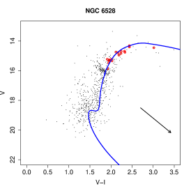
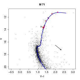
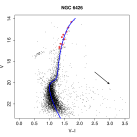
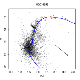
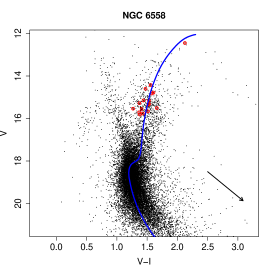
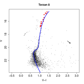
Figure 1: Colour-Magnitude diagrams of all clusters analysed in the present work. Left panels are metal-rich clusters, middle panels are intermediate metallicity clusters and right panels correspond to the more metal-poor ones. All stars within 2 $\times$ r_half-light are plotted, without any cleaning procedure. Dartmouth isochrones with literature parameters (Table 2) are overplotted. Selected RGB stars for spectroscopic observations are in red. Reddening vectors are shown in each CMD based on E(B-V) listed in Table 2.

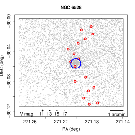
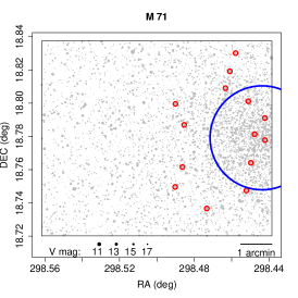
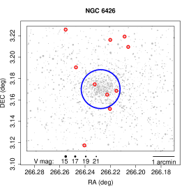
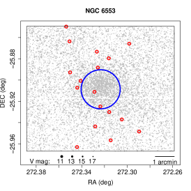
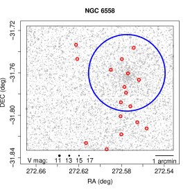
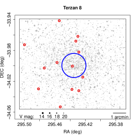
Figure 2: Sky map of all clusters analysed in the present work. Panels are displayed as in Figure 1. Only brightest stars are shown, and the size of the dots are scaled with the stars magnitudes as indicated in each plot. Selected RGB stars for spectroscopic observations are in red. The blue circle corresponds to the half-light radius of each cluster from Table 2.

The spectra were taken using the grism 1400V, centred at 5200 Å, covering the range 4560 - 5860 Å, with a resolution of R$\sim$2,000. Figure 3 illustrates the spectra of a metal-poor and a metal-rich red giant star, where many of the strongest lines are indicated.

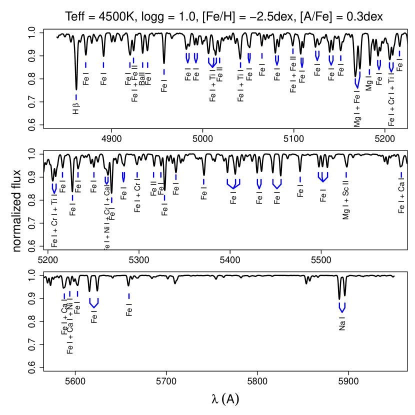
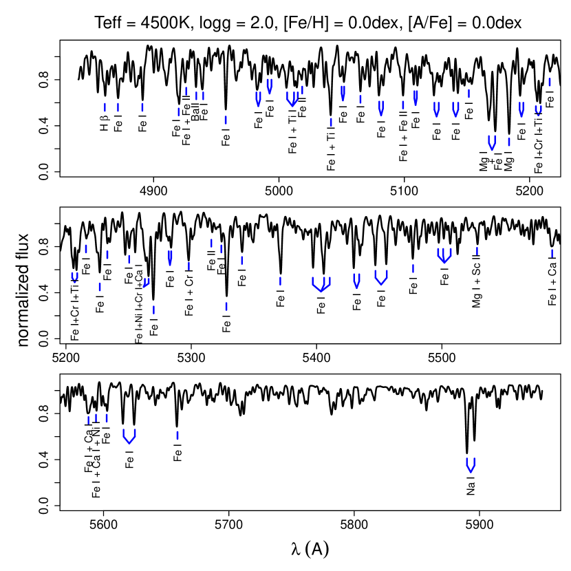
Figure 3: Identification of most important atomic lines in each strong feature of spectra with FORS2 resolution (R$\sim$2,000). The most important molecular band in this region is MgH around $\lambda$ = 5165 ${\rm\AA}$, on top of the Mg I triplet lines. Left panel shows a metal-poor red giant star from Coelho et al. (2005) library, and right panel shows a metal-rich one. The left panels were zoomed in the y-axis direction for better visualization.

The spectra were reduced using esorex/FORS2 pipeline with default parameters for bias and flatfield correction, spectra extraction, and wavelength calibration. The only modification relative to default parameters, has been the introduction of a list of skylines, since the default list had only one line. The wavelength calibration proved to be satisfactory with such line list. A last step in the reduction procedure was a manual removal of cosmic rays.

3 Stellar parameters derivation

3.1 Radial velocities

Radial velocities were measured using the ETOILE code through cross correlation with a template spectrum from the chosen library. Tests were done in order to check the results, by measuring radial velocities using fxcor@IRAF (cross correlation), and rvidlines@IRAF (using wavelength of MgI triplet lines as a reference). The derived velocities are consistent, therefore we used ETOILE also to determine radial velocities. A mean FWHM of arc lines of 2.36$\pm$0.04Å (125 km/s) was measured. This leads to a radial velocity uncertainty of $\sim$13 km/s. Heliocentric radial velocities for each star can be found in Table LABEL:starinfo, where the last column refers to the values measured from the CaII triplet (CaT) lines in the near infrared by Saviane et al. (2012) for member stars for NGC 6528, NGC 6553, M 71 and NGC 6558, and by Vasquez et al. (2014 in prep.) for NGC 6426 and Terzan 8. There is good agreement between the present radial velocity values and those from the CaT line region. A few exceptions are stars #8 of NGC 6558, #2, #10 of M 71, among others. A possible explanation for this could be due to a not perfectly centred source in the slit in some cases, as suggested by Katz et al. (2011) in using CFHT-MOS. Average values for member stars in each cluster are presented in Figure 4, where our results are compared to CaT results (Saviane et al., 2012 and Vasquez et al., in prep.), and with Harris (1996, 2010 edition) catalogue. Error bars from the literature are smaller than the empty circles that represent literature v_helio, except for NGC 6426, as can be seen in Figure 4. Our results are in good agreement with both references. In particular, the radial velocity measured for NGC 6426 is in agreement between this work and CaT results based on individual member stars, but it is only compatible with the literature value within 3$\sigma$. The explanation is that the only work that measured radial velocities for this cluster was based on integrated light from photographic plates (Hesser et al., 1986). Therefore, the present radial velocity derivation for NGC 6426 is more reliable.

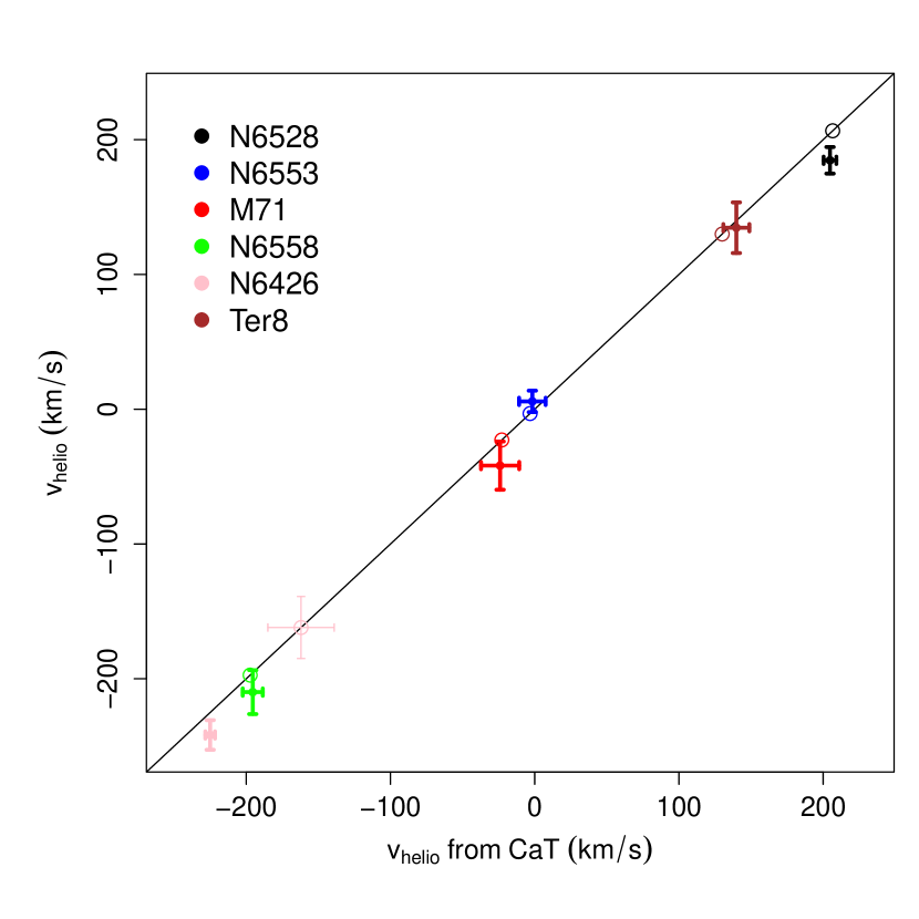
Figure 4: Average of heliocentric radial velocities of member stars (see details in Section 4.3 and values in Table LABEL:starinfo) for each globular cluster. Our results are plotted against those from CaT spectroscopy (Saviane et al., 2012) and Vasquez et al. (in prep.) showing good agreement. Error bars are the standard deviation of the average. One-to-one line is plotted for visual guidance, where radial velocities from Harris (1996, 2010 edition) are overplotted as empty circles.

3.2 Atmospheric parameters

Full spectrum fitting with minimum distance method is employed, using the ETOILE code described in Katz et al. (2011) and Katz (2001). We apply the calculations to the wavelength region 4600-5600 Å, similarly to the procedure described in Katz et al. (2011).

Automated derivation of the atmospheric parameters (T_eff, log($g$), [Fe/H], [$\alpha$/Fe]) of a stellar spectrum is carried out by comparing the target spectrum with each library spectrum, thus covering a large range of atmospheric parameters. In each comparison, ETOILE fits the template spectrum to the observed spectrum. Mathematically, ETOILE solves, by least squares, for the polynomial by which to multiply the template spectrum to minimize the differences with the observed spectrum (see Equations 1 and 2). The aim of these operations is to compensate for the differences between the template and observed spectra which are not from stellar origin: e.g. flux level/normalisation, instrumental profile, interstellar reddening. In particular, concerning this last point, no explicit reddening is applied to the template. The differential reddening correction is included in the fitting of the template to the observed spectrum.

$$S=\sqrt{\sum\limits_{i=0}^{n}{\bigg{\{}F_{\rm obs}(i)-\Big{[}\sum\limits_{j=0}^{m}{u_{j}\cdot\big{(}\lambda(i)-\lambda_{\rm central}\big{)}^{j}}\Big{]}\cdot F_{\rm templ}(i)\bigg{\}}^{2}}}$$ (1)

where $n$ is the number of pixels in the spectrum being analysed, $F_{\rm obs}(i)$ and $F_{\rm templ}(i)$ are the fluxes of the analysed and the template spectra respectively pixel by pixel (i.e. lambda by lambda), $m$ is the order of the polynomial that multiplies $F_{\rm templ}(i)$ and $u_{j}$ are the coefficients, $\lambda_{\rm central}=[\lambda(0)+\lambda(n)]/2$. Equation 1 is minimized to find the multiplicative polynomial that minimizes the differences in flux between observed and template spectra solving the $m+1$ Equations below. In this work we adopted $m=4$.

$$\frac{\partial S}{\partial u_{j}}=0{\rm\ ,\ where\ }j\in\{0,...,m\}$$ (2)

After determination of the polynomial that minimizes the difference between each template and the observed spectrum, as defined by Equation 1, templates are ranked in order of increasing $S$ and the parameters of the top N templates are averaged out to produce the final results. Determination of the optimal value of N is discussed in Section 3.2.2. This is called the similarity method introduced by Katz et al. (1998). For a more detailed explanation see Katz (2001).

Before running the code, two important steps are needed: to convolve all the library spectra to the same resolution of the target spectra, and to correct for radial velocities $v_{r}$. Convolution calculations were performed for the library spectra using the task GAUSS in IRAF. The code ETOILE measures the radial velocities by comparison with template spectra from the library, a reliable way to measure $v_{r}$ in each observed spectrum and correct them.

Figure 5 shows six examples of spectral fitting, for a metal-poor (Terzan8_11), a metal-rich (NGC6528_11) and an intermediate metallicity star (NGC6558_7) using COELHO and MILES templates. The template stars that best fit these cluster stars among the available spectra from MILES library are BD+060648, HD161074 and HD167768, respectively. For COELHO the best templates are the ones with the following parameters: (T_eff, log(g), [Fe/H]) = (5000K, 2.5, -2.0), (3500K, 0.0, -1.5) and (5000K, 3.0, -1.0), respectively. The residuals shown at the bottom of each panel indicate that the metal-poor target spectrum is similar to the template spectrum within 2% for both libraries, except for a few strong features. The residuals for the metal-rich star shows a similarity between target and template spectra of 5% for MILES and of 7% for COELHO, except for the boundaries $\lambda\gtrsim 5700$ Å and $\lesssim 4700$ Å, and for a few strong features. For the intermediate metallicity star the residuals present a sigma of 3% for both libraries with few stronger features varying more than 3%. These differences between the spectra are reflected in the atmospheric parameters, and they are compensated by taking the average of parameters of the most similar spectra. For Terzan8_11, there are 8 MILES spectra close enough which were averaged, for NGC6528_11, 21 MILES spectra were considered, and for NGC6558_7 it were found 8 stars. For all cases with COELHO library 10 templates were considered in the average. Details on the criterion to select the number of template spectra are discussed in Section 3.2.2.

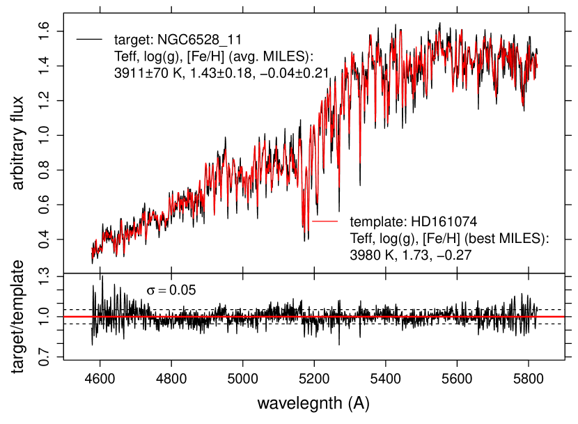
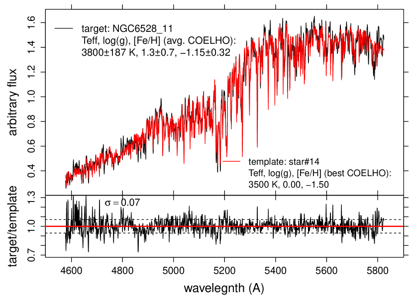
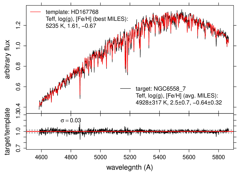
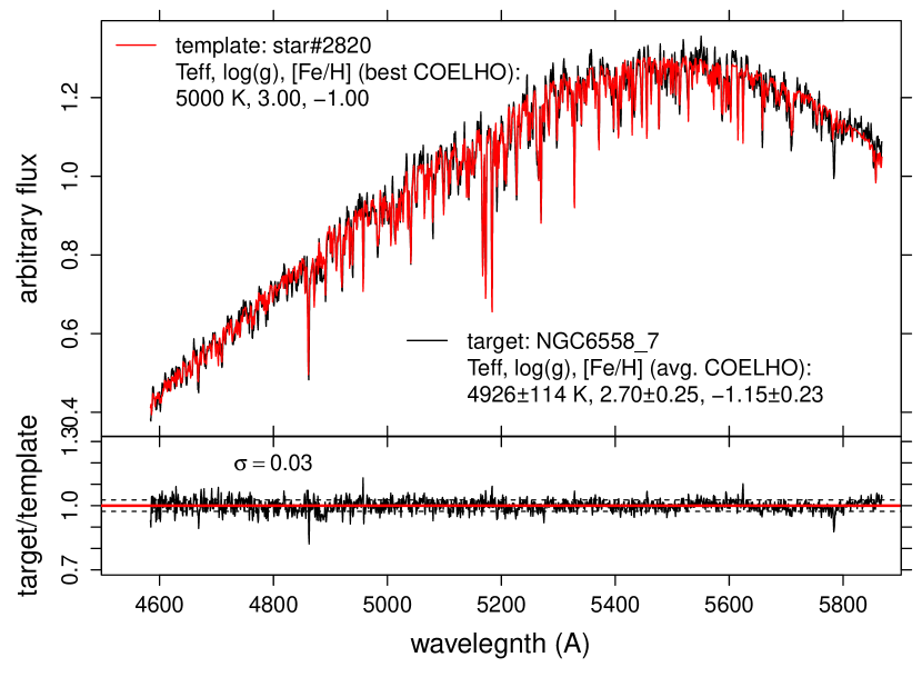
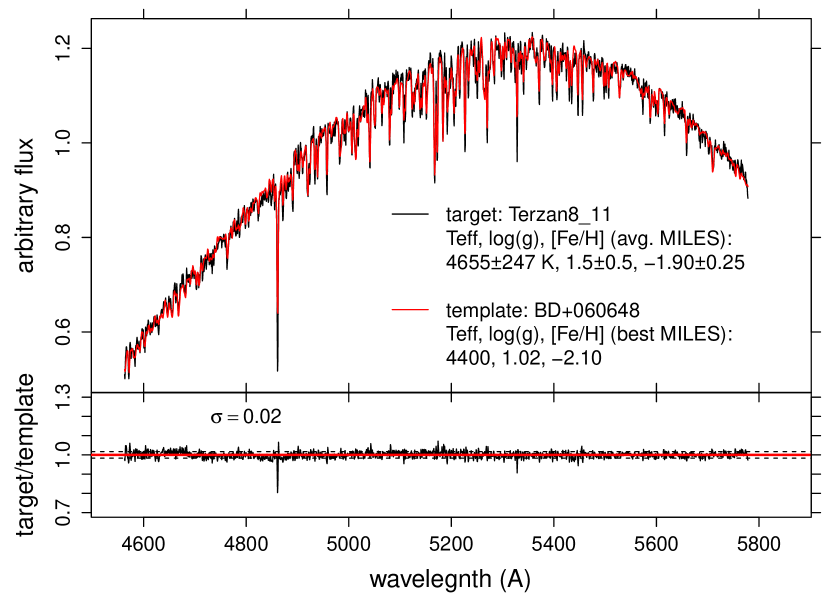
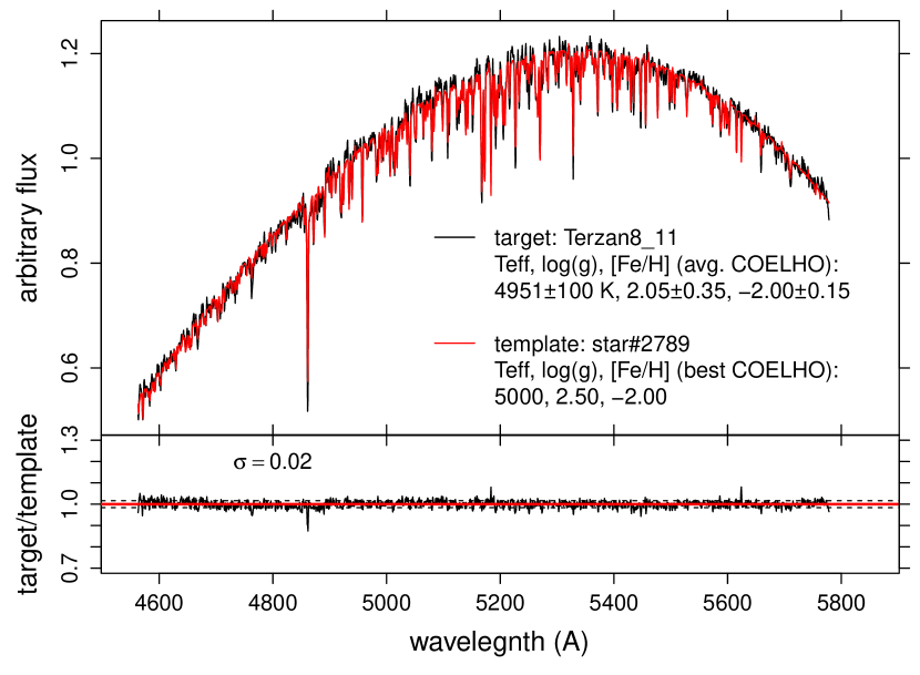
Figure 5: Examples of spectral fitting carried out with ETOILE for a metal-rich (NGC6528_11), an intermediate metallicity (NGC6558_7) and a metal-poor (Terzan8_11) star in the upper, middle and bottom panels, respectively. Left panels represent the best fits using MILES template spectra, and in the right panel the best fits using COELHO spectra are shown. For each star, its spectrum (black line) is overplotted by the template spectrum (red line) that best fits it. Below each stellar spectrum the residuals of each fit are presented. The match between the spectra is done following the procedures explained in Section 3.2. The fit appears very satisfactory for the whole wavelength interval for all cases. In each comparison we give the parameters of the template spectrum and of the average parameters using only MILES or only COELHO spectra for each star, as presented in Table LABEL:finalparam.

3.2.1 Stellar libraries

The core of the atmospheric parameters derivation in this work is the choice of a stellar library. There are two classes of stellar libraries: based on observed or synthetic spectra. The real spectra are more reliable, but the drawback is that they have abundances typical of nearby stellar populations. The synthetic libraries have no noise, and a large and uniform coverage of the atmospheric parameters space, however there are still limitations on the completeness of atomic and molecular line lists, plus uncertainties on oscillator strengths, and assumptions on atmospheric models, such as 1-D and local thermodynamical equilibrium. For these reasons, it is useful to use both observational and synthetic libraries. In the present work, we use two libraries, one observed and one synthetic, as described below:

The MILES library (Sánchez-Blázquez et al., 2006) has 985 stellar spectra with resolution R$\sim$2 080@5 200 Å, and mean signal-to-noise ratio of 150 per pixel for field and open cluster stars, and 50 for globular cluster stars. Atmospheric parameters coverage is (Cenarro et al., 2007; Milone et al., 2011):

$$\begin{array}[]{rcccl}352.5{\rm nm}&<&\lambda&<&750{\rm nm}\\ 2\,747{\rm K}&<&T_{\rm eff}&<&36\,000{\rm K}\\ -0.20&<&{\rm log}(g)&<&5.50\\ -2.86&<&{\rm[Fe/H]}&<&+1.65\\ -0.54&<&{\rm[Mg/Fe]}&<&+0.74\\ \end{array}$$

The COELHO library (Coelho et al., 2005) has 6367 synthetic stellar spectra with wavelength steps of 0.02Å (resolution R=130 000@5 200 Å). Atmospheric parameters coverage is:

$$\begin{array}[]{rcccl}300{\rm nm}&<&\lambda&<&1800{\rm nm}\\ 3\,500{\rm K}&<&T_{\rm eff}&<&7\,000{\rm K}\\ 0.0&<&{\rm log}(g)&<&5.0\\ -2.5&<&{\rm[Fe/H]}&<&+0.5\\ 0.0&<&{\rm[\alpha/Fe]}&<&+0.4\\ \end{array}$$

where $\alpha$-elements considered in this library are: O, Mg, Si, S, Ca and Ti.

Given that all cluster stars are located in the red giant branch, as shown in Figure 1, we selected only stars in this region in the parameters space of the libraries (see Figure 6) to avoid non-physical results.

Figure 6: HR diagram showing the parameter space available from the MILES library. Dartmouth isochrones (Dotter et al., 2008) are overplotted for metallicities close to those of the six analysed globular clusters: [Fe/H] = -0.1, -0.8, -1.3, -2.2 dex, with [$\alpha$/Fe] = 0.2, 0.4, 0.4, 0.4, 0.4 dex, respectively, and ages = 13 Gyr for all cases. Colours of the dots indicate the metallicity range closer to the isochrones. Dashed black lines are the adopted limit to select RGB stars from MILES used as reference for the fits.

3.2.2 Average results and errors: validation with well-known stars

We define different criteria for MILES and COELHO libraries for taking the average of stellar parameters from reference spectra, as mentioned in Section 3.2. For MILES the average results are based on different numbers of templates depending on the sampling as shown in Figure 6. For the synthetic library COELHO the sampling is homogeneous, therefore a constant number of templates is adopted. We found that 10 templates for COELHO cover satisfactorily the variations in the four stellar parameters (T_eff, log($g$), [Fe/H] and [$\alpha$/Fe]). The COELHO library was built by varying all alpha-elements (O, Mg, Si, S, Ca, Ti) together, therefore [$\alpha$/Fe] is an average of the effect from enhancement of these element abundances.

The criterion to define average results from the MILES library is more complex, as follows. The code provides a list of the closest reference spectra from the library, ranked by the similarity parameter ($S$, as defined in Equations 1 and 2). The final parameters T_eff, log($g$), [Fe/H] and [Mg/Fe] are the average of the parameters of first N reference stars from the ETOILE output, where N depends on the sampling of the library for each combination of parameters. The average is weighted by $1/S^{2}$ as shown in the equation below for T_eff (the same is valid for the other three parameters):

$$\centering{\rm T}_{\rm eff}\ (N)=\frac{\sum\limits_{i=1}^{N}{{\rm T}_{\rm eff,i}\times\frac{1}{S_{i}^{2}}}}{\sum\limits_{i=1}^{N}{\frac{1}{S_{i}^{2}}}}\@add@centering$$ (3)

The errors are defined as the average of the squared residuals, weighted by $1/S^{2}$, as shown in the equation below for T_eff (the same is valid for the other three parameters). For N=1, we adopted the same error of N=2.

$$\centering\sigma_{{\rm T}_{\rm eff}\ (N)}=\sqrt{\frac{\sum\limits_{i=1}^{N}{({\rm T}_{\rm eff,i}-{\rm T}_{\rm eff})^{2}\times\frac{1}{S_{i}^{2}}}}{\sum\limits_{i=1}^{N}{\frac{1}{S_{i}^{2}}}}}\@add@centering$$ (4)

To estimate the number of reference stars to be averaged in each case, we proceeded with some tests using 59 spectra of 49 well-known stars, listed in Table LABEL:tab:etoilevalidation. These stars were selected among red giant stars (same log($g$) and T_eff intervals defined in Figure 6) presented in the ELODIE library (Prugniel et al., 2007). Stellar spectra were taken from ELODIE library and convolved to the FORS2 resolution. Reference atmospheric parameters were averaged from the PASTEL catalogue (Soubiran et al., 2010), and the quality filter was determined by a threshold in the standard deviation: $\sigma_{T_{\rm eff}}<200$K, $\sigma_{\rm log(g)}<0.5$, $\sigma_{\rm[Fe/H]}<0.2$. We calculated the average parameters and respective errors for different N and compared the results with the average values of T_eff, log($g$), [Fe/H] from the PASTEL catalogue (Soubiran et al., 2010). We minimize the equation below to find the best N that will give the final parameters and respective errors. This equation considers the distance between the average for a given N and literature average; in this way all the three parameters are minimized at the same time. Milone et al. (2011) have measured [Mg/Fe] for MILES spectra, therefore it is possible to take averages for this parameter as a function of N, and use [Mg/Fe] for the best N as an estimation of the $\alpha$-enrichment for each star.

$$\begin{array}[]{ll}{\rm RR}_{\rm tot}\ (N)=&\sqrt{{\rm RR_{\rm N}}({\rm T}_{\rm eff})^{2}+{\rm RR_{\rm N}}({\rm log}(g))^{2}+{\rm RR_{\rm N}}({\rm[Fe/H]})^{2}}\\ \end{array}$$ (5)

where RR_N(T_eff) is given by the equation below (the same is valid for the other three parameters):

$${\rm RR_{\rm N}}({\rm T}_{\rm eff})=\frac{{\rm T}_{\rm eff}\ (N)-{\rm T}_{\rm eff}^{(lit)}\ (N)}{{\rm T}_{\rm eff}^{(lit)}\ (N)}$$ (6)

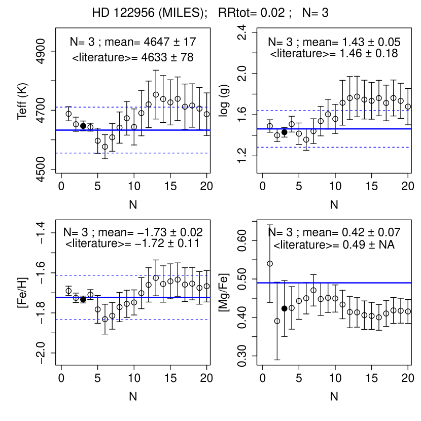
Figure 7: Finding procedure of N for the case of star HD122956, based on the minimization of the residuals of T_eff, log($g$) and [Fe/H] (equation 5). Circles represent the averages of the parameters of N best reference stars. Filled black circle indicates the closest values to the references. Blue solid lines and blue dashed lines are average from PASTEL catalogue and standard deviation (Table LABEL:tab:etoilevalidation). For this star, Fulbright (2000) published [Mg/Fe] and we compare also with the averages as a function of N. All the four parameters for the best N=3 are compatible with literature.

Figure 7 illustrates the finding procedure of N for the case of star HD122956, showing that ETOILE could recover all the four parameters accurately. The resulting parameters, RR_tot, N, and literature values are presented in Table LABEL:tab:etoilevalidation. Different stars need different number N of templates to find the best result. Moreover the ratio $S$(N)/$S$(1) for the best N is roughly constant for all ETOILE template spectra, with an average value of 1.1$\pm$0.1. The best number N and the respective ratio $S$(N)/$S$(1) are related to the library sampling, for example, for a given star with best N=1 it means that there is only one reference star with $S$(N)/$S$(1) $\lesssim$ 1.1, and there are two possible explanations: either the target star matches perfectly some reference star, or the library has no other reference spectra similar enough to that star to be considered. In the cases with N=15, for instance, the library has 15 reference spectra very similar ($S$(N)/$S$(1) $\lesssim$ 1.1) to the target spectra, and their parameters must be averaged in order to get the parameters for the target star.

All results are plotted in Figure 8 showing the good agreement of ETOILE results and PASTEL catalogue average for T_eff, log($g$), [Fe/H] in the whole range for RGB stars analysed in this work. The behaviour of the derived values of [Mg/Fe] vs. [Fe/H] has a similar behaviour to field stars (see e.g. Figure 6 of Alves-Brito et al., 2010).

Figure 8: Comparison of the parameters determined in this work with PASTEL catalogue average values for the well-known stars presented in Table LABEL:tab:etoilevalidation. These plots endorse the usage of ETOILE code for atmospheric parameters determination for red giant stars in the optical spectral region. Only stars with $\sigma_{T_{\rm eff}}<200$K, $\sigma_{\rm log(g)}<0.5$, $\sigma_{\rm[Fe/H]}<0.2$ from PASTEL catalogue were selected as good quality candidates for validation of the method. Below the plots of T_eff, log($g$) and [Fe/H] there is a residuals plot and the dispersion of the residuals is displayed in the respective plots.

After these tests we can consider that ETOILE code together with the MILES library works well for low-resolution spectra of red giant stars in the optical region. Additionally we define the criterion to consider a reference spectrum similar enough to be considered in the average of the parameters as $S$(N)/$S$(1) $\leq$ 1.1.

4 Results

The derived T_eff, log($g$), [Fe/H], [Mg/Fe] or [$\alpha$/Fe] are presented in Table LABEL:finalparam. In order to discuss these results, we proceed as follows: in Sect. 4.1 we plot T_eff and log($g$) for stars in each cluster together with isochrones of age and metallicity given in Table 2. Section 4.2 compares [Fe/H] with CaT results from Saviane et al. (2012) and Vasquez et al. (in prep.). Subsequently all checked parameters are used to select member stars for each cluster (Section 4.3). Finally, all parameters for member stars are compared individually with high-resolution analysis, when available in the literature. M 71 and NGC 6558 have three stars in common with Cohen et al. (2001), and Barbuy et al. (2007) respectively, and Terzan 8 has four stars in common with Carretta et al. (2014), as described in Sections 4.4.1, 4.4.2 and 4.4.3, respectively. For NGC 6528, NGC 6553 and NGC 6426 we did not find any star in common with high-resolution spectroscopic studies.

4.1 T_eff, log($g$) against isochrones

In high-resolution spectroscopy studies, usually T_eff is estimated from photometry and log($g$) from theoretical equations. These parameters are employed as initial guesses to derive [Fe/H], which is applied to redetermine T_eff and log($g$) iteratively, until reaching a convergence of the three parameters. In this work we fit all the three parameters at the same time (Section 3.2), and a check on these parameters is carried out as explained below.

Figure 9 displays the results of all stars in the six clusters in a Hertzprung-Russell diagram form. Left, middle and right panels show the results using MILES library, COELHO library and the average of both results, respectively. Black dots represent member stars of each cluster, and grey dots are not members, based on the selection described in the next Section 4.3. Dartmouth isochrones (Dotter et al., 2008) with age, [Fe/H] and [$\alpha$/Fe] from Table 2 are overplotted in the diagrams of Figure 9 in blue. Cyan lines have the same age and [Fe/H] as the respective blue lines, but with the extreme values of [$\alpha$/Fe] = -0.2 and +0.8, available from the models.

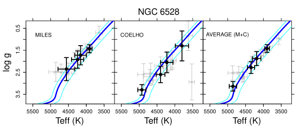
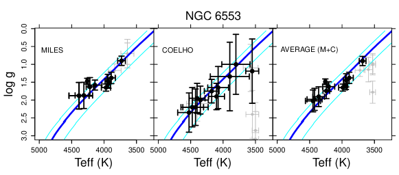
Figure 9: Comparison of T_eff and log($g$) of stars in each cluster with Dartmouth isochrones (Dotter et al., 2008) for the metal-rich clusters NGC 6528 and NGC 6553. For each cluster we show the results based on MILES and COELHO libraries and a third panel with the weighted average of the results from both libraries. The parameters of age, [Fe/H] and [$\alpha$/Fe] for the blue thick isochrones were taken from Table 2. Cyan thin isochrones have same age and [Fe/H] as blue ones, but with the limits [$\alpha$/Fe] = -0.2dex and +0.8dex. Black dots represent member stars of each cluster, and grey dots are not members.

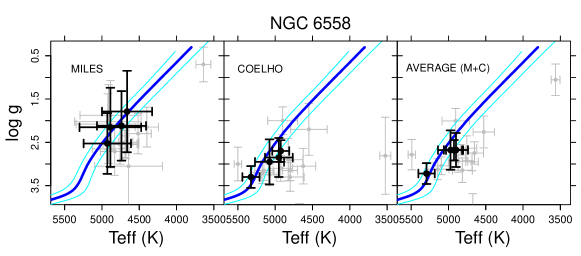
Figure 10: Same as Figure 9 for the two clusters with intermediate metallicity M 71 and NGC 6558.

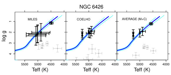
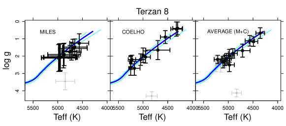
Figure 11: Same as Figure 9 for the two metal-poor clusters NGC 6426 and Terzan 8.

The results on T_eff and log($g$) from MILES and COELHO are in good agreement with the isochrones. We also computed an average of the results weighted by their uncertainties that are displayed in the right panels of Figure 9. For reasons explained in Section 4.2, we adopted as the final results in this work the weighted average of MILES and COELHO results.

4.2 Comparison of [Fe/H] with CaT results

In the comparisons of results from CaT and the optical spectra, it is important to keep in mind the facts that: The synthetic spectra in the optical reproduce less well the metal-rich stars, given the missing opacity due to millions of very weak lines, not taken into account in the calculations; this blanketing effect lowers the continuum in real stars, and the measurable lines are shallower than in the present synthetic spectra calculations by Coelho et al. which makes metal-rich stars more similar to synthetic spectra slightly more metal-poor. On the other hand, CaT-based abundances also suffer from significant uncertainties. The modelling of the CaT region is affected by contamination by TiO lines and NLTE effects. Moreover, measuring a CaT index is very difficult, in particular for more metal-rich and luminous stars with the blanketing effect mentioned above, which complicates the definition of the continuum for equivalent widths (EW) measurements. The conversion of the EW to [Fe/H] has larger uncertainties which could recover even higher [Fe/H] for metal-rich stars. Another difficulty to measure EW for metal-rich ([Fe/H] $\gtrsim$ -0.7, 47 Tuc) is to choose the best function to fit the line profile: Gaussian, Gaussian+Lorentzian or Moffat, while for lower metallicities only a Gaussian function works well. This further step could introduce uncertainties in [Fe/H] from CaT in metal-rich regime. A further issue is that the ratio between [Ca/H] vs. [Fe/H] is not solar, i.e., since Ca is an alpha-element, it is enhanced in old stars, even if not as enhanced as O and Mg. Detailed discussion about CaT metallicities can be found in Saviane et al. (2012). On the other hand, there are some advantages to compare our results with CaT: a) all selected stars from photometry were observed both in the near-infrared (CaT, Saviane et al., 2012 and Vasquez et al. in prep.) and in the optical spectral region which is very good for comparisons of the whole sample at once; b) The CaT-based metallicities were calibrated with the Carretta et al. (2009) metallicity scale which makes CaT metallicities valid at least up to [Fe/H] $<$ -0.43 (the most metal-rich cluster observed by Carretta et al., 2009, NGC 6441), with caution for metallicities higher than that. Finally, the optical region studied here is suitable to provide robust values of [Fe/H] for each cluster, to be compared with the CaT value, and to converge ultimately to the average [Fe/H] for each cluster.

Figure 12 shows the comparisons of the metallicity values presented in Table LABEL:finalparam with those from CaT analysis. Upper left panel shows that [Fe/H] using MILES library is in good agreement with CaT results for the three most metal-rich clusters NGC 6528, NGC 6553 and M 71. This is in agreement with the sampling of metal-rich stars for all combinations of T_eff and log($g$) as displayed in Figure 6 in red and green. For NGC 6558 with [Fe/H]$\sim$-1.0 the dispersion on the parameters is larger which is explained by the smaller number of stars available in the library with such metallicity. MILES is based on the solar neighbourhood showing therefore only a few stars with [Fe/H]$\sim$-1.0. For the metal-poor clusters NGC 6426 and Terzan 8 the library sampling is even more sparse, as becomes evident in Figure 6. In this case, the average of parameters from the library takes into account some more metal-rich reference stars which results in higher values of [Fe/H] for NGC 6426 and Terzan 8 stars.

Metallicities using COELHO library are compared with CaT results in the upper right panel of Figure 12. The synthetic spectra reproduce less well the metal-rich stars, given the missing opacity as mentioned above. Because of this effect, stars of NGC 6528, NGC 6553 and M 71 are more metal-poor than CaT results. On the other hand, COELHO library is suitable to reproduce the stars of the three more metal-poor clusters of this sample, NGC 6558, NGC 6426 and Terzan 8.

To summarize, for the three more metal-rich clusters, MILES results are better, and for the other three, COELHO results are preferable. The bottom right panel of Figure 12 shows the concatenation of this conclusion, i.e., it displays MILES results for NGC 6528, NGC 6553 and M 71, and COELHO results for NGC 6558, NGC 6426 and Terzan 8. An alternative combination of results from MILES and COELHO is to take the average of the results weighted by their uncertainties. This average combines the best of both libraries and gives a good correlation with CaT results, as shown in the bottom left panel of Figure 12. Both criteria to combine MILES and COELHO (two bottom panels) are in good agreement with CaT results, and we adopted [Fe/H] from the average results represented in the bottom left panel.

We adopted as final parameters the mean of MILES and COELHO results, because they show better compatibility with the isochrones for T_eff and log($g$), and with the CaT results for metallicities. We recall that CaT-based metallicities were calibrated in the Carretta et al. (2009) scale.

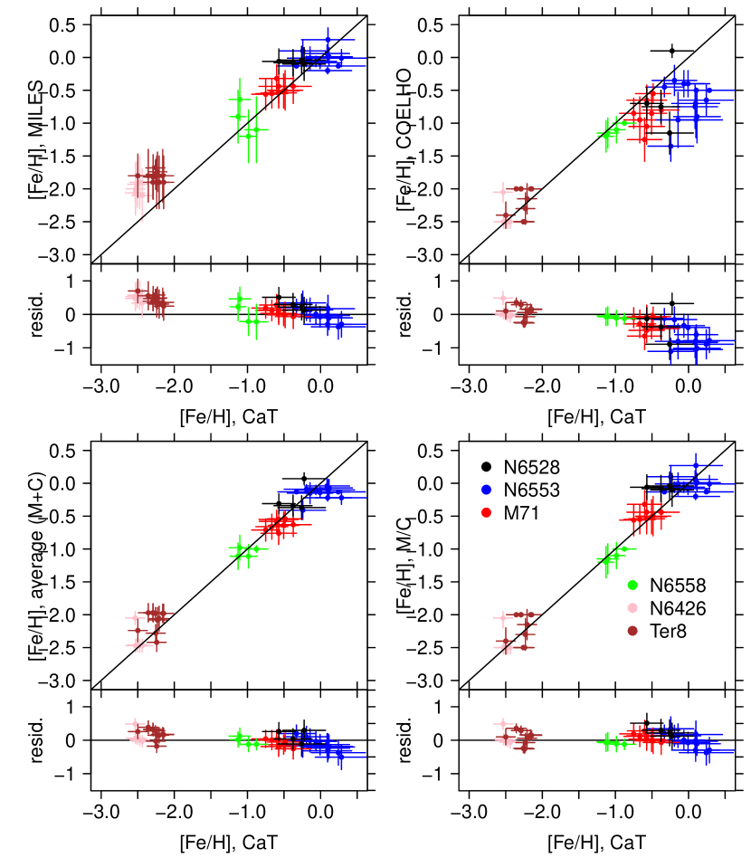
Figure 12: Comparison of [Fe/H] from this work (mean of MILES and COELHO, see Table LABEL:finalparam) with those from equivalent widths of Ca II triplet for the same stars with the same instrument by Saviane et al. (2012) and Vasquez et al. (in prep). Upper panels compare CaT metallicities with those obtained with MILES and COELHO libraries. Bottom panels are two types of combination of the results: average of each star on the left, and assuming MILES results for more metal-rich and COELHO results for more metal-poor stars, on the right. Below the plots there is a residuals plot.

4.3 Membership selection

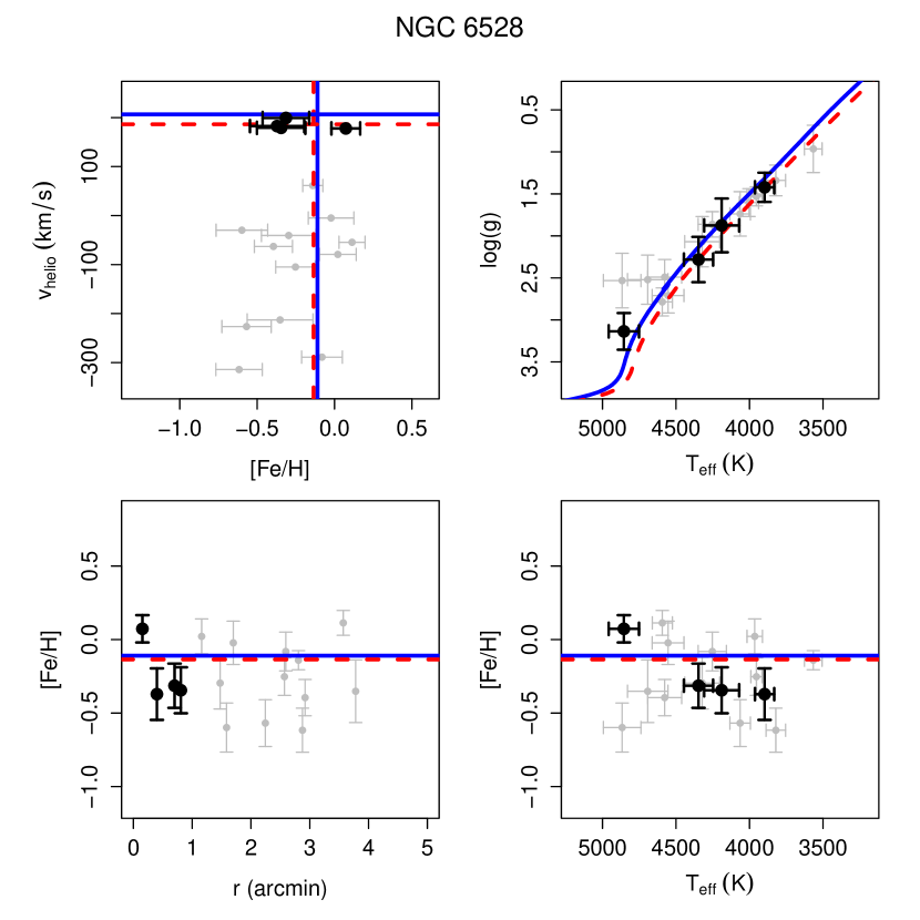
Figure 13: Step-by-step of selection of member stars for NGC 6528. Black dots are selected member stars, grey dots are non-members and green circles shows stars considered as cluster member by Saviane et al. (2012) but non-members in the present work. Blue solid lines are drawn based on values of Table 2, which were also applied to the ischrones from Dotter et al. (2008). Red dashed lines refer to the weighted average of the member stars parameters.

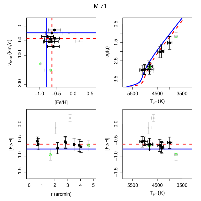
Figure 14: Same as Figure 13 for M 71.

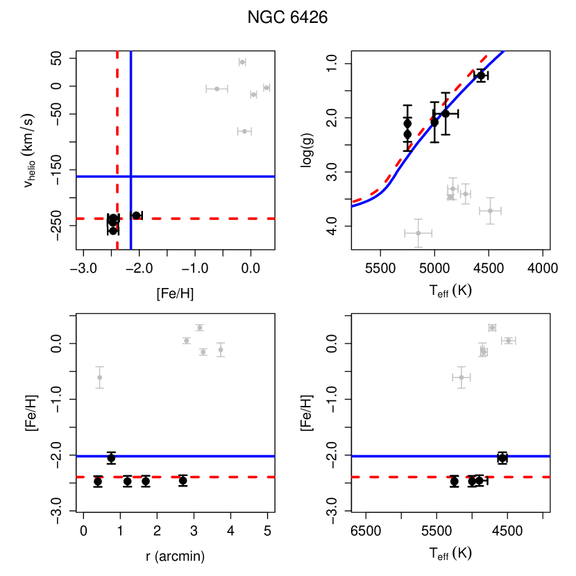
Figure 15: Same as Figure 13 for NGC 6426.

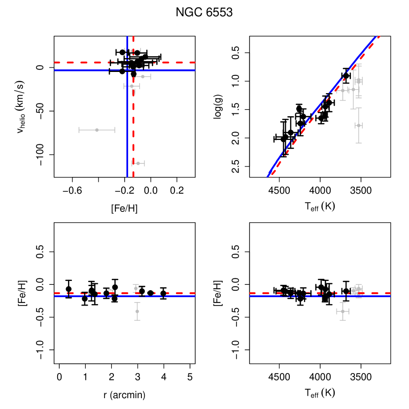
Figure 16: Same as Figure 13 for NGC 6553.

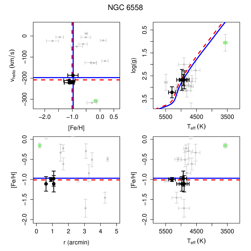
Figure 17: Same as Figure 13 for NGC 6558.

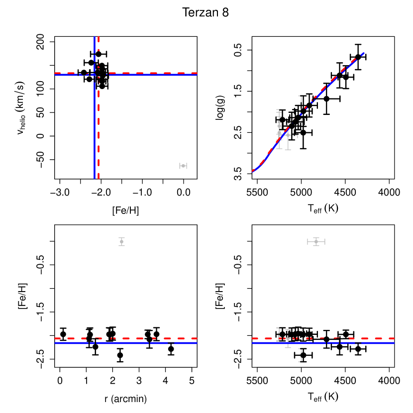
Figure 18: Same as Figure 13 for Terzan 8.

In Figure 13 we show four panels for each globular cluster. In upper left panels radial velocities against metallicities are displayed (this is the classical plot for membership selection for globular clusters, e.g. Zoccali et al., 2008). Blue solid lines are parameters from Table 2 and red dashed lines are the average of parameters for cluster members only (for isochrones we use age, [Fe/H] and [$\alpha$/Fe] information). For all clusters there is a clear concentration of stars around literature values, and we considered as members stars with v${}_{\rm helio}<\pm 2\sigma$ ($\sigma$ is given in Sect. 3.1) of the literature value, and with [Fe/H] $<\pm 0.3$ dex. Upper right panels show T${\rm eff}$ vs. log($g$) compared with Dartmouth isochrones (Dotter et al., 2008) as done in Sect. 4.1. Blue solid lines are isochrones with parameters from Table 2, and red dashed lines are based on the average (Table 5) of the parameters for member stars (Table LABEL:finalparam). All member stars are close to the isochrones, confirming the membership selection. This extra criterion led to the exclusion of a few more stars from the v${\rm helio}$-[Fe/H] selection. Also excluded in some cases are stars cooler than T_eff $<$ 4000 K that give a poor fit to template spectra due to TiO bands. Bottom left panels show [Fe/H] against distance to the cluster centre, and no trends were found for any sample cluster. Bottom right panels show no correlation between T_eff and [Fe/H] for any of the six clusters analysed in this work.

In conclusion all T${\rm eff}$, log($g$) and [Fe/H] values are found to sit in well defined sequences following the isochrones. Bottom-right panels show no correlation between [Fe/H] and T${\rm eff}$, suggesting that the [Fe/H]/T${\rm eff}$ degeneracy does not affect our fitting procedure. Further evidence of this is provided by the comparisons of our results with [Fe/H] measures from high-resolution analysis available in the literature, presented in Sections 3.2.2, 4.4.1, 4.4.2 and 4.4.3.

Table 5: Final average parameters for member stars in each globular cluster, and respective internal errors.

Cluster	$<$v${}_{\rm helio}>$ (km/s)	$<$[Fe/H]$>^{(a)}$	$<$[Fe/H]$>^{(b)}$	$<$[Fe/H]$>^{(avg)}$	$<$[Mg/Fe]$>^{(a)}$	$<$[$\alpha$/Fe]$>^{(b)}$
NGC 6528	185$\pm$10	-0.07$\pm$0.10	-0.18$\pm$0.08	-0.13$\pm$0.05	0.05$\pm$0.09	0.26$\pm$0.05
NGC 6553	6$\pm$8	-0.125$\pm$0.009	-0.55$\pm$0.07	-0.133$\pm$0.017	0.107$\pm$0.009	0.302$\pm$0.025
M 71	-42$\pm$18	-0.48$\pm$0.08	-0.77$\pm$0.08	-0.63$\pm$0.15	0.25$\pm$0.07	0.293$\pm$0.032
NGC 6558	-210$\pm$16	-0.88$\pm$0.20	-1.02$\pm$0.05	-1.012$\pm$0.013	0.26$\pm$0.06	0.23$\pm$0.06
NGC 6426	-242$\pm$11	-2.03$\pm$0.11	-2.46$\pm$0.05	-2.39$\pm$0.11	0.38$\pm$0.06	0.24$\pm$0.05
Terzan 8	135$\pm$19	-1.76$\pm$0.07	-2.18$\pm$0.05	-2.06$\pm$0.17	0.41$\pm$0.04	0.21$\pm$0.04

4.4 Validation with high-resolution spectroscopy

We found stars in common with literature high-resolution spectroscopy for three clusters: M 71, NGC 6558 and Terzan 8. In Sect. 4.3 we were able to identify ten member stars of M 71, five member stars of NGC 6558, and twelve member stars in Terzan 8, these being the same selected by Saviane et al. (2012), and Vasquez et al. (in prep.). The derived stellar parameters are reported in Table LABEL:finalparam for member and non-member stars. We were able to find detailed analyses in the literature for 3 member stars in M 71, 3 in NGC 6558 and 4 in Terzan 8, as reported below.

4.4.1 M 71

Cohen et al. (2001) observed 25 member red giant stars of M 71 using HIRES@Keck (R$\sim$34,000), and derived their T_eff and log($g$). In two subsequent papers, they derived [Fe/H] (Ramírez et al., 2001) and [Mg/Fe] (Ramírez & Cohen, 2002) for them. We have three stars in common that are presented in Table 7. Temperature and gravity values are compatible within 0.5 to 2-$\sigma$, [Fe/H] and [Mg/Fe] are compatible within 0.1 to 1.5-$\sigma$.

Table 7: Final atmospheric parameters for the three stars of M 71 in common with Cohen et al. (2001), and also their determinations for the respective parameters.

Star	Teff (K)	log($g$)	[Fe/H]	[Mg/Fe]
	Teff-C01 (K)	log($g$)-C01	[Fe/H]-C01	[Mg/Fe]-C01
M71_7	3997$\pm$89	1.53$\pm$0.35	-0.58$\pm$0.17	0.15$\pm$0.18
1-45	3950	0.9	-0.60$\pm$0.03	0.43$\pm$0.09
M71_9	4316$\pm$87	1.97$\pm$0.33	-0.76$\pm$0.17	0.27$\pm$0.21
1-64	4200	1.35	-0.61$\pm$0.03	0.43$\pm$0.09
M71_13	4808$\pm$106	2.82$\pm$0.24	-0.63$\pm$0.18	0.23$\pm$0.20
G53476_4543	4900	2.65	-0.61$\pm$0.03	0.36$\pm$0.06

4.4.2 NGC 6558

Barbuy et al. (2007) observed six RGB stars using the high-resolution (R$\sim$22,000) spectrograph FLAMES+GIRAFFE@VLT/ESO, and derived T_eff, log($g$), [Fe/H], and [Mg/Fe] for each of them. We have three stars in common with their sample: #6, #8, #9, corresponding to their identification as B11, F42, F97, respectively (see Table 8). For stars #6 and #9, full spectrum fitting recovers all parameters within 1-$\sigma$. Star #8 is a more complicated case because it is a very cool star (T${}_{\rm eff}<4000$ K) and molecular bands of TiO are important. They change a lot the continuum which is not fitted perfectly. In fact, the derived parameters for this star led us to select it as non-member. Although temperature agrees with that from Barbuy et al. (2007), the gravity is much lower than their results.

These results show that full spectrum fitting method is reliable, consistent among all libraries, and present reasonable errors for RGB stars hotter than $\sim$4000 K. Stars cooler than that must be analysed with a better suited reference library, cointaining a sufficient number of cool stars at all metallicities.

Table 8: Final atmospheric parameters for the three stars of NGC 6558 in common with Barbuy et al. (2007), and also their determinations for the respective parameters.

Star	Teff (K)	log($g$)	[Fe/H]	[Mg/Fe]
	Teff-B07 (K)	log($g$)-B07	[Fe/H]-B07	[Mg/Fe]-B07
6558_6	4899$\pm$162	2.68$\pm$0.39	-1.11$\pm$0.20	0.22$\pm$0.07
B11	4650	2.2	-1.04	0.20
6558_8	3565$\pm$ 59	1.05$\pm$0.36	-0.16$\pm$0.06	0.23$\pm$0.00
F42	3800	0.5	-1.01	0.30
6558_9	4972$\pm$168	2.68$\pm$0.46	-1.11$\pm$0.18	0.41$\pm$0.16
F97	4820	2.3	-0.97	0.23

4.4.3 Terzan 8

Carretta et al. (2014) observed six stars with UVES@VLT/ESO (R$\sim$45,000) and 14 with GIRAFFE@VLT/ESO (R$\sim$22,500 - 24,200), with among them four stars in common with our FORS2@VLT/ESO sample. Their parameters for these stars are presented in Table 9. For temperature and gravity the compatibility is within 1 to 3-$\sigma$, except for T_eff of star Ter8_8 which is in the limit of 3.9-$\sigma$ of distance. For [Fe/H] all stars have compatible values with Carretta et al. (2014) within 1-$\sigma$, except for star Ter8_1 which is in the limit of 3.9-$\sigma$ of distance. [Mg/Fe] is compatible within 1-$\sigma$.

Table 9: Final atmospheric parameters for the four stars of Terzan 8 in common with Carretta et al. (2014), together with their determinations for the respective parameters.

Star	Teff (K)	log($g$)	[Fe/H]	[Mg/Fe]
	Teff-C14 (K)	log($g$)-C14	[Fe/H]-C14	[Mg/Fe]-C14
Ter8_1	5067$\pm$314	2.24$\pm$0.30	-1.97$\pm$0.14	0.40$\pm$0.13
2913	4628	1.49	-2.52$\pm$0.07	0.58
Ter8_4	4354$\pm$88	0.67$\pm$0.31	-2.28$\pm$0.13	0.40$\pm$0.14
2357	4188	0.66	-2.29$\pm$0.10	0.48$\pm$0.14
Ter8_8	5151$\pm$108	2.56$\pm$0.36	-2.06$\pm$0.19	0.40$\pm$0.18
2124	4730	1.67	-2.28$\pm$0.26	0.56
Ter8_9	4564$\pm$94	1.12$\pm$0.30	-2.24$\pm$0.17	0.42$\pm$0.13
1658	4264	0.80	-2.40$\pm$0.07	0.51$\pm$0.02

Differently from M 71 and NGC 6558, the comparison between our results and Carretta et al. (2014) for Terzan 8 give all three parameters T_eff, log($g$) and [Fe/H] systematically larger. For this reason we inspected the T_eff-log($g$) diagram of both sets of data, compared with the Dartmouth (Dotter et al., 2008), PARSEC (Bressan et al., 2012) and BASTI (Pietrinferni et al., 2004) isochrones, as shown in Figure 19. The Carretta et al. (2014) results are compatible with an isochrone of [Fe/H] = -1.7, [$\alpha$/Fe]=+0.4 and 13 Gyr, whereas the present results fit better with an isochrone [Fe/H] = -2.2, [$\alpha$/Fe]=+0.4 and 13 Gyr. Except for star Terzan8_4 showing very similar gravities, for the other stars they are different. Given that are results are consistent with isochrones, we suggest that in the high-resolution analysis of metal-poor stars, the effect ofver-ionization at low temperature atmospheres, may have led to lower gravities.

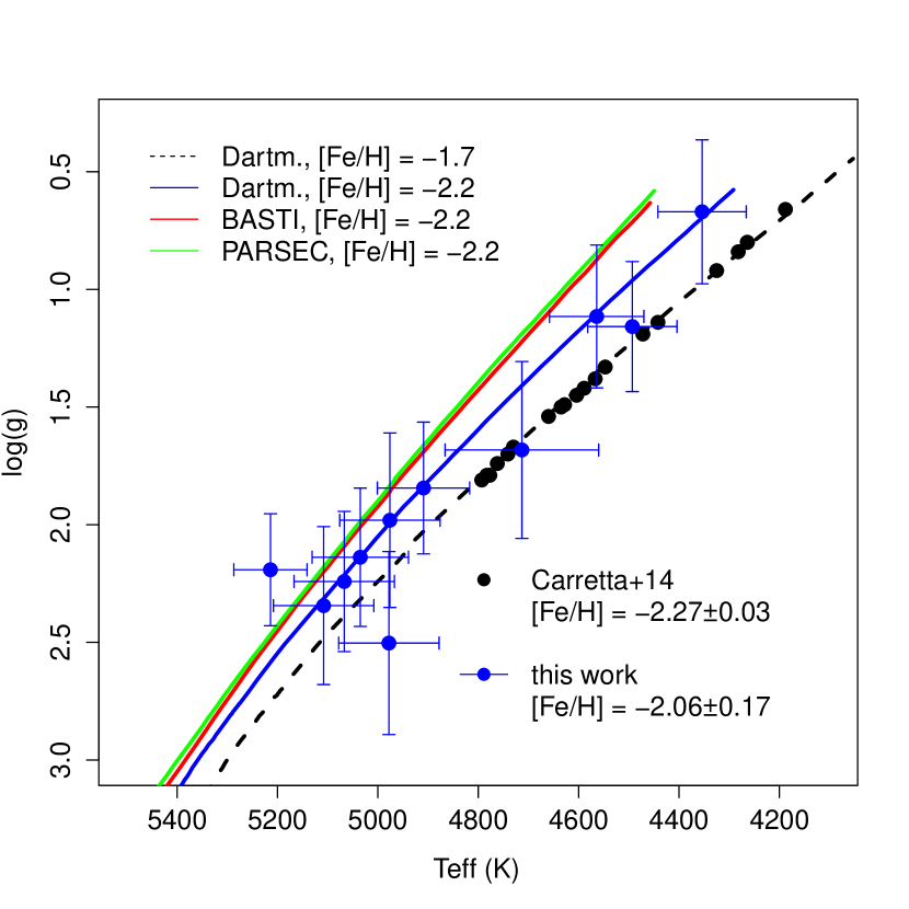
Figure 19: Diagram log($g$) vs. T${\rm eff}$ for Terzan 8 showing present (blue points with error bars) and Carretta et al. (2014, black filled circles) results, overplotted with Dartmouth, PARSEC and BASTI isochrones for ages = 13 Gyr, and metallicities indicated on the Figure.

5 Discussion

Results for individual stars in each cluster (Table LABEL:finalparam) and average results (Table 5) are discussed below and compared with literature results. Figure 20 displays the comparison of our [Fe/H] results for each cluster with reference values, showing good agreement for the whole range of metallicities from [Fe/H] = -2.5 to solar. Figure 21 gives the comparison of the average results of [Fe/H] and [Mg/Fe] with abundances for field stars of the different Galactic components: bulge, thin/thick disc and inner/outer halo. We discuss case by case below.

Figure 20: Comparison of [Fe/H] from this work (Table 5) with those from literature, as revised in Table 2. Error bars are the weighted average of the [Fe/H] of member stars in each cluster, as presented in Table LABEL:finalparam. For NGC 6553 and NGC 6558 the error bars are not visible because they are too small (see Table 5). In the lower panel the residuals are shown.

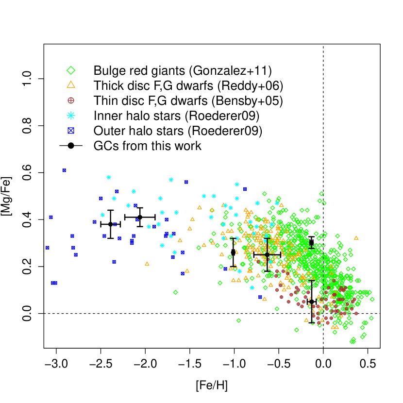
Figure 21: Chemical evolution of the Milky Way based on bulge field stars (Gonzalez et al., 2011), thin disc (Bensby et al., 2005), thick disc (Reddy et al., 2006), inner and outer halo (Roederer, 2009). Results from this work for globular clusters are overplotted. For NGC 6553 the point corresponds to [$\alpha$/Fe] instead of [Mg/Fe], as discussed in Section 5.2

5.1 Metal-rich clusters NGC 6528, NGC 6553

NGC 6528 and NGC 6553 have similar CMDs (Ortolani et al., 1995), as shown in Figure 1. Their metallicities and element abundance ratios are also similar for most elements, as reported in Table 10. As given in Table 2 they have reddening E(B-V) = 0.54 mag and 0.63 mag, [Fe/H] = -0.11 and -0.18, [Mg/Fe] = 0.24 and 0.26, respectively. They are located in the Milky Way bulge, distant 0.6 kpc and 2.2 kpc from the Galactic centre, and in opposite “southern legs” of the X-shaped bulge (see Figure 3 of Saito et al., 2011). Figure 9 shows that ETOILE recovers parameters for member stars coherent with a simple stellar population represented by the isochrones. Although all the results are compatible between the libraries, error bars for MILES results are lower than from COELHO results. This synthetic library, on the other hand, gives better alpha-enhancement values compatible with average values from high-resolution studies ([$\alpha$/Fe] = 0.26$\pm$0.05 and 0.302$\pm$0.025, respectively, from Table 5). In particular these values are compatible with NGC 6553 (Alves-Brito et al., 2006, Cohen et al., 1999), whereas for NGC 6528 the alpha-enhancement is lower (Zoccali et al., 2004 ). In this respect, MILES cannot give an alpha-enhancement, since their metal-rich stars are basically solar neighbourhood stars, that have no alpha-enhancement for metal-rich stars (see Figure 2 in Milone et al., 2011). The results from MILES are [Mg/Fe] = 0.05$\pm$0.09 and 0.107$\pm$0.009, respectively. This is a particularity of the bulge, where stars are metal-rich and old. As mentioned above, Zoccali et al. (2004) find [Mg/Fe]=+0.07 from high-resolution spectroscopy of three stars of NGC 6528, which is compatible with MILES and not with COELHO. For N6553, Cohen et al. (1999) finds [Mg/Fe]=+0.41 also from high-resolution spectroscopy of five stars, which is closer to COELHO results.

Figure 13 compares the final results (average of MILES and COELHO results) with isochrones with literature parameters (same as Figure 9) and an additional isochrone considering the parameters derived from this work (Table 5). The isochrones consider [$\alpha$/Fe] from COELHO results as discussed above. We derived [Fe/H] = -0.13$\pm$0.06 and -0.133$\pm$0.009 for NGC 6528 and NGC 6553, respectively, in agreement with high spectral resolution analyses of Carretta et al. (2001) and Alves-Brito et al. (2006).

Table 10: Literature abundances in NGC 6528 and NGC 6553.

[Fe/H]	[O/Fe]	[Mg/Fe]	[Si/Fe]	[Ca/Fe]	[Ti/Fe]	[Na/Fe]	[Eu/Fe]	[Ba/Fe]	[Mn/Fe]	[Sc/Fe]	ref.
NGC 6528
+0.07	+0.07	+0.14	+0.36	+0.23	+0.03	+0.40	—	+0.14	$-$0.37	$-$0.05	(1)
$-$0.11	+0.10	+0.05	+0.05	$-$0.40	$-$0.25	+0.60	—	—	—	—	(2)
NGC 6553
$-$0.16	+0.50	+0.41	+0.14	+0.26	+0.19	—	—	—	—	-0.12	(3)
$-$0.20	+0.20	—	—	—	—	—	—	—	—	—	(4)
$-$0.20	—	+0.28	+0.21	+0.05	$-$0.01	+0.16	+0.10	$-$0.28	—	—	(5)

5.2 Moderately metal-rich clusters M 71, NGC 6558

According to Harris (1996, 2010 edition), M 71 (or NGC 6838) is located 6.7 kpc from the Galactic centre, with a perpendicular distance to the Galactic plane of only 0.3 kpc towards the South Galactic Pole, which means that this globular cluster is located in the Milky Way disc. Because of that its reddening is high, although not as high as for most bulge clusters, with E(B-V) = 0.25. NGC 6558 is located only 1.0 kpc from the Galactic centre, in particular between the two “southern legs” of the X-shaped bulge (see Figure 3 of Saito et al., 2011). It has a reddening of E(B-V) = 0.44. Although they are located in different components of the Milky Way, these clusters share similar metallicities, [Fe/H]$\sim$-0.8, and [Fe/H]$\sim$-1.0, respectively.

Figure 1 shows a red horizontal branch (HB) for M 71 and a blue HB for NGC 6558, and this difference is not due to metallicity (Lee et al., 1994). It is true that a few other parameters can change the HB morphology at a fixed metallicity, as discussed by Catelan et al. (2001), for instance, but in this case the age is probably playing the major role. Literature ages are 11 Gyr (VandenBerg et al., 2013) and 14 Gyr old (Barbuy et al., 2007), respectively. M 71 is younger and moderately metal-rich, therefore a red horizontal branch is expected. In particular, we derived a slightly higher metallicity for this cluster in comparison with the literature, [Fe/H] = -0.63$\pm$0.06. NGC 6558 has a high metallicity for such a blue horizontal branch, and Barbuy et al. (2007) argue that if this is interpreted as pure factor of age, this cluster should be one of the oldest objects in the Milky Way. We derived [Fe/H] = -1.01$\pm$0.04, compatible with their findings ([Fe/H] = -0.97$\pm$0.15), and more metal-rich than Harris (1996, 2010 edition) value of [Fe/H] = -1.32. Saviane et al. (2012) also found [Fe/H] = -1.03$\pm$0.14 for NGC 6558 from their Ca II triplet spectroscopy, with error being dominated by the external calibration uncertainty.

Comparing the error bars of T_eff and log($g$) in Figure 9 between the two libraries, for M 71 they are of the same order, but for NGC 6558 MILES results present larger error bars. The main reason for this is that MILES library is based on solar neighbouhood stars, and only a few of them have metallicities [Fe/H] $\approx$ -1.0 (see Figure 2 of Sánchez-Blázquez et al., 2006). Synthetic libraries such as that of Coelho et al. (2005) have spectra for any combination of atmospheric parameters evenly distributed in the parameter space. Therefore COELHO library is more suitable for the analysis of these moderately metallicity clusters.

For this range of metallicity and for expected values of [Mg/Fe] from the literature (0.19 and 0.24, respectively), MILES and COELHO results are compatible, as shown in Table 5, [Mg/Fe] = 0.25$\pm$0.07 and 0.26$\pm$0.06, [$\alpha$/Fe] = 0.293$\pm$0.032 and 0.23$\pm$0.06, respectively. Ramírez & Cohen (2002) give an average [Mg/Fe]=+0.37 from 24 stars observed with high-resolution in M71, which is compatible with our findings. The number of stars in MILES with these metallicities is low, but it is sampled enough for determinations of [Fe/H] and [Mg/Fe] for Milky Way stars. COELHO spectra have [$\alpha$/Fe] varying from 0.0 to 0.4, which is also enough for this kind of objects.

5.3 Metal-poor clusters NGC 6426, Terzan 8

NGC 6426 and Terzan 8 present similar CMDs with a same literature age and metallicity of 13 Gyr (Dotter et al., 2011; VandenBerg et al., 2013) and [Fe/H] = -2.15 (Harris, 1996, 2010 edition). NGC 6426 is located in the northern halo of the Milky Way, 14.4 kpc from the Galactic centre and 5.8 kpc above the Galactic plane. Its height is much larger than the height scale of the thick disc (0.75 kpc, de Jong et al., 2010), but it has a non-negligible reddening of E(B-V) = 0.36, at a galactic latitude of b=16.23^∘. The best CMD available for this cluster was observed with the ACS imager onboard the Hubble Space Telescope by Dotter et al. (2011), and they derived an age of 13.0$\pm$1.5 Gyr from isochrone fitting. Our pre-image photometry based on observations with the Very Large Telescope/ESO produced a rather well-defined CMD for this cluster which is compatible with a 13 Gyr isochrone (see Figure 1).

Terzan 8 is located in the southern halo of the Milky Way, 19.4 kpc from the Galactic centre and 10.9 kpc below the Galactic plane. It has the lowest reddening of all clusters analysed in this work, E(B-V) = 0.12. This is one of the four Milky Way globular clusters believed to be captured from the Sagittarius dwarf galaxy (Ibata et al., 1994), the other three being M 54, Terzan 7 and Arp 2 (Da Costa & Armandroff, 1995). Carretta et al. (2014) did not find a strong evidence for Na-O anticorrelation, typical for globular clusters which may indicate that these clusters may have simple stellar populations.

Atmospheric parameters derived in this work for both clusters are in good agreement with literature values, when compared to the isochrones in Figure 9. As for the moderately metal-rich clusters, MILES results present larger error bars than COELHO results for T_eff and log($g$), and the reason is the same as mentioned above, i.e., the sampling of MILES library is poorer for this metallicity range (see Figure 2 of Sánchez-Blázquez et al., 2006). Derived metallicities for these clusters are [Fe/H] = -2.39$\pm$0.04 and -2.06$\pm$0.04, respectively. For NGC 6426 our determination is 0.24 more metal-poor than given in Harris’s catalogue ([Fe/H] = -2.15). However the only derivation of the metallicity for this cluster was done by Zinn & West (1984) based on integrated light ([Fe/H] = -2.20$\pm$0.17) which is compatible with our findings. The value from Harris catalogue was obtained by applying the Carretta et al. (2009) metallicity scale. We present for the first time a direct measurement of metallicity of individual red giant stars finding a more metal-poor value than previously attributed to this cluster. Terzan 8 is compatible with the Harris (2010 edition) catalogue of [Fe/H] = -2.16. There are three papers with metallicities for this cluster: Mottini et al. (2008) and Carretta et al. (2014), based on high-resolution spectra of individual star and average metallicity [Fe/H] = -2.35$\pm$0.04 and -2.27$\pm$0.08, respectively. The third paper is Da Costa & Armandroff (1995) who derived [Fe/H] = -1.99$\pm$0.08 based on CaII triplet spectroscopy. Our result is compatible with the more metal-rich results.

For alpha-enhancement in this metallicity range, MILES spectra goes up to [Mg/Fe] = 0.74, while COELHO is limited to the models of [$\alpha$/Fe] = 0.4. The results based on COELHO ([$\alpha$/Fe] = 0.24$\pm$0.05 and 0.21$\pm$0.04, respectively) are less enhanced than MILES ([Mg/Fe] = 0.38$\pm$0.06 and 0.41$\pm$0.04, respectively), the latter being closer to literature abundance ratios.

6 Summary and conclusions

We present a method of full spectrum fitting, based on the ETOILE code, to derive v_helio, T_eff, log($g$), [Fe/H], [Mg/Fe] and [$\alpha$/Fe] for red giant stars in Milky Way globular clusters. The observations were carried out with FORS2@VLT/ESO with resolution R$\sim$2,000.

We validated the method using well known red giant stars covering the parameter space of 4000 K $<$ T_eff $<$ 6000 K, 0.0 $<$ log($g$) $<$ 4.0, -2.5 $<$ [Fe/H] $<$ +0.3 and -0.2 $<$ [Mg/Fe] $<$ +0.6. The spectra of these reference stars are from the ELODIE library and the parameters from the PASTEL catalogue. The parameters were recovered for the whole range of parameters. We applied the method to red giant stars, and the code ETOILE has been applied and validated also for dwarf stars by Katz et al. (2011).

In order to establish the methodology to be adopted for a larger sample of clusters, we chose two metal-rich (NGC 6528, NGC 6553), two moderately metal-rich (M 71, NGC 6558) and two metal-poor (NGC 6426 and Terzan 8) clusters. NGC 6528, NGC 6553 and NGC 6558 are located in the bulge, M 71 in the disc, NGC 6426 and Terzan 8 in the halo. For all clusters the effective temperatures and gravities are well determined using the MILES and Coelho et al. (2005) libraries of spectra. Metallicities and alpha-element enhancement are also derived with the caveats that for alpha-enhanced bulge clusters with [Fe/H] $>$ -0.5, MILES is not suitable, since it has only solar neighbourhood stars, therefore in this case we use COELHO results because synthetic libraries have all combinations of parameters. For [Fe/H] $\approx$ -1.0 MILES has few stars due to a lack of such stars in the solar vicinity. For metal-poor clusters, with high [$\alpha$/Fe], MILES may be more suitable than COELHO because the latter is limited to 0 $<$ [$\alpha$/Fe] $<$ 0.4dex, if such high Mg enhancements are confirmed.

The present results are in agreement with literature parameters available for five of the six template clusters. NGC 6426 is analysed for the first time using spectroscopy of individual stars. Therefore we provide a more precise radial velocity of -242$\pm$11 km/s, a metallicity [Fe/H] = -2.39$\pm$0.04, and [Mg/Fe] = 0.38$\pm$0.06. The comparison of our results of [Fe/H] and [Mg/Fe] to those from field stars from all Galactic components shows that the globular clusters follows the same chemical enrichment pattern as the field stars.

In conclusion, full spectrum fitting technique using ETOILE code together with MILES and COELHO libraries appears to be suitable to derive chemical abundances for Milky Way globular clusters, from low/medium-resolution spectra of red giant branch stars. Depending on the stellar population studied, the choice of library with parameter space covering the expected values for the clusters is a crucial ingredient, observed library being better for more metal-rich stars and synthetic library being preferable for the more metal-poor ones. This method will be applied to the other Milky Way globular clusters from this survey. It is also promising for extragalactic stars, that can be more easily observed with similar resolutions of R$\sim$2,000, for studies of galaxy formation and evolution.

Table 11: Star by star coordinates, magnitude, colour, heliocentric radial velocity. Velocities from CaT were taken from from Saviane et al. (2012) for NGC 6528, NGC 6553, M 71 and NGC 6558, and from Vasquez et al. (2014, in prep.) for NGC 6426 and Terzan 8.

Star ID	RA (J2000)	DEC (J2000)	V	V-I	vhelio	vhelio-CaT	members
	(deg)	(deg)	(mag)	(mag)	(km/s)	(km/s)
NGC6528_2	271.1807715771910	-30.0070234836130	15.987	1.982	-51.55	—
NGC6528_3	271.1933667526377	-30.0114575457940	15.647	2.836	61.28	—
NGC6528_4	271.1789935185810	-30.0172537974630	15.596	2.257	-314.24	—
NGC6528_5	271.1883528713980	-30.0237445060760	15.939	1.937	-226.44	—
NGC6528_6	271.1974416677920	-30.0295599638440	17.060	1.741	-4.93	—
NGC6528_7	271.2102328036860	-30.0372195159180	15.887	2.140	-79.24	—
NGC6528_8	271.2027175539120	-30.0434602130820	16.428	1.831	179.09	200	M
NGC6528_9	271.1969387171677	-30.0500739849720	16.501	1.774	199.18	208	M
NGC6528_10	271.2070341687930	-30.0537176170110	16.145	2.007	177.87	209	M
NGC6528_11	271.2013524700317	-30.0600904185180	15.511	2.255	182.67	202	M
NGC6528_13	271.1879324598030	-30.0747465095010	16.429	1.731	-29.84	—
NGC6528_14	271.2012738946260	-30.0802412070160	16.032	2.056	-40.56	—
NGC6528_15	271.1774205888063	-30.0879237445260	15.892	2.062	-288.86	—
NGC6528_16	271.1843122189650	-30.0926974725130	15.954	2.150	-104.91	—
NGC6528_17	271.1904270294383	-30.1021087576640	16.537	1.844	-62.96	—
NGC6528_18	271.1726747862950	-30.1092237523470	16.666	1.767	-212.87	—
NGC6528_19	271.1832358189100	-30.1108940656500	16.468	1.778	-54.47	—
NGC6553_1	272.3536106669400	-25.8497112721910	15.816	2.109	3.90	-8	M
NGC6553_3	272.3507085422689	-25.8636412811220	15.832	2.010	16.71	19	M
NGC6553_4	272.2982167426244	-25.8658039783470	15.310	2.618	-71.71	-39	M
NGC6553_5	272.3267021788947	-25.8733214097360	15.775	2.522	12.23	-12	M
NGC6553_6	272.3161974470756	-25.8795540059450	16.237	2.177	0.81	-6	M
NGC6553_7	272.3258216397713	-25.8883122417460	15.338	2.881	6.76	3	M
NGC6553_8	272.3501542761960	-25.8928074210270	15.370	3.088	18.98	—
NGC6553_9	272.3409674217040	-25.9007568498840	16.253	2.097	-27.72	-32	M
NGC6553_10	272.3439213760840	-25.9071903257530	15.985	1.998	2.34	2	M
NGC6553_11	272.3287891424960	-25.9110912319810	15.441	2.443	10.12	-3	M
NGC6553_13	272.3235733284760	-25.9249134402580	15.906	2.075	-4.38	-12	M
NGC6553_14	272.3157993633750	-25.9300477560180	15.187	2.382	5.40	-5	M
NGC6553_15	272.3047106358403	-25.9370597367310	14.980	2.996	-21.36	—
NGC6553_16	272.3280756666470	-25.9436286781210	15.708	2.332	17.42	8	M
NGC6553_17	272.2895515368990	-25.9484055025060	15.065	2.849	-110.00	—
NGC6553_18	272.3144982937293	-25.9566926017970	15.407	3.681	-10.44	—
NGC6553_19	272.3440933085433	-25.9630097530170	15.843	2.209	-7.38	-4	M
M71_2	298.4578984488130	18.8301452486084	14.606	1.269	-150.46	-34	M
M71_4	298.4609554670447	18.8192204176758	13.030	1.503	-53.75	-41	M
M71_5	298.4632902665389	18.8090499016740	14.391	1.282	-52.74	-26	M
M71_6	298.4900822754500	18.7995866372160	13.534	1.367	-44.07	-37	M
M71_7	298.4510869475747	18.8011235588184	12.376	1.719	-69.84	-34	M
M71_8	298.4854008510480	18.7869940682184	14.421	1.280	-51.13	—
M71_9	298.4422411559920	18.7910962573810	13.146	1.530	-35.78	-24	M
M71_10	298.4476878071520	18.7813713381542	12.140	2.042	-129.33	-26	M
M71_13	298.4496765965810	18.7641970806387	14.281	1.303	-23.72	-5	M
M71_14	298.4902210311380	18.7496150618418	14.582	1.210	-13.11	-17	M
M71_15	298.4521026881480	18.7474809643955	14.580	1.209	-41.62	-8	M
M71_16	298.4732927595957	18.7366583486676	14.727	1.231	-23.67	—
NGC6558_3	272.6225545017980	-31.7335169754310	16.862	1.434	-6.32	—
NGC6558_4	272.5685475821600	-31.7363376028500	16.541	1.441	-38.29	—
NGC6558_5	272.6214120279947	-31.7468917846890	16.349	1.360	-23.46	—
NGC6558_6	272.5796695743913	-31.7469946267620	15.982	1.524	-210.85	-196	M
NGC6558_7	272.5899712149563	-31.7570504471050	15.803	1.393	-186.59	-187	M
NGC6558_8	272.5739816190383	-31.7605125893880	13.651	2.044	-307.26	-210	M
NGC6558_9	272.5637020636180	-31.7666306345590	16.026	1.499	-221.66	-204	M
NGC6558_10	272.5771880085779	-31.7733227718450	16.710	1.580	-21.13	—
NGC6558_11	272.5757815235553	-31.7788392433250	16.753	1.329	-220.56	-195	M
NGC6558_12	272.5805489015007	-31.7879129654280	16.521	1.452	-126.79	—
NGC6558_13	272.5717825299750	-31.7916739864870	15.626	1.477	-127.74	—
NGC6558_14	272.5809044425367	-31.8010529051890	16.740	1.188	-118.59	—
NGC6558_15	272.5652668675210	-31.8066271885810	16.480	1.293	105.58	—
NGC6558_16	272.5564861827613	-31.8124812867920	16.366	1.450	-316.32	—
NGC6558_17	272.5801632324050	-31.8180552937480	16.964	1.348	-49.93	—
NGC6558_18	272.6131914789087	-31.8262981571080	16.911	1.288	11.27	—
NGC6558_19	272.5939188278727	-31.8321512784620	17.013	1.299	-5.38	—
NGC6426_1	266.2553357204670	3.2257821720617	18.018	1.359	-80.97	-49.927
NGC6426_2	266.2088188480099	3.2192772570129	17.597	1.394	-2.85	11.325
NGC6426_3	266.2200960712349	3.2161573577027	16.468	1.586	-15.18	12.662
NGC6426_4	266.2059346355020	3.2095717676480	16.072	1.644	-236.29	-230.019	M
NGC6426_7	266.2472044411759	3.1904905620518	17.666	1.459	-259.55	-225.413	M
NGC6426_9	266.2324246578110	3.1746245634344	17.170	1.515	-244.78	-222.660	M
NGC6426_10	266.2152297889280	3.1685396261324	15.544	1.749	-231.87	-221.297	M
NGC6426_11	266.2225277929239	3.1649406775723	17.892	1.354	-4.92	12.270
NGC6426_13	266.2203523684530	3.1516328071727	16.745	1.482	-236.15	-225.730	M
NGC6426_18	266.2405437043161	3.1175053813749	16.970	1.434	43.08	72.570
Terzan8_1	295.4542164758450	-33.9415478435970	16.706	1.232	134.45	138.8238	M
Terzan8_4	295.4999075670249	-33.9726804796670	15.268	1.436	120.63	137.4998	M
Terzan8_5	295.4297741922069	-33.9618073863440	17.002	1.135	134.61	152.6001	M
Terzan8_6	295.4324851623650	-33.9679803480730	17.517	1.076	119.81	138.3819	M
Terzan8_8	295.4284871648290	-33.9821965410250	17.089	1.108	173.81	150.6620	M
Terzan8_9	295.4571652028810	-33.9956864225960	15.447	1.352	155.67	139.3673	M
Terzan8_10	295.4738836006140	-34.0028288269560	17.381	1.076	-63.09	-25.6758
Terzan8_11	295.4369091804230	-34.0003943267700	15.682	1.277	142.74	150.6086	M
Terzan8_13	295.4233824419659	-34.0145360437400	17.364	1.101	149.42	144.2031	M
Terzan8_14	295.4815071780459	-34.0298070702590	15.530	1.388	116.26	131.9558	M
Terzan8_15	295.4375324314209	-34.0304794278020	16.433	1.219	105.77	121.5507	M
Terzan8_16	295.4285209120099	-34.0321898355090	16.778	1.122	128.12	140.9906	M
Terzan8_18	295.4529047094940	-34.0531331777060	16.143	1.273	134.81	131.1500	M

Table 11: continued.

Table 12: List of 49 well known stars selected from ELODIE spectral library. Literature parameters are average from PASTEL catalogue. Results from this work are using MILES library. See details in Section 3.2.2.

ELODIE	Star	RRtot	N	Slim	Teff (K)	log($g$)	[Fe/H]	Teff (K)	log$g$	[Fe/H]	[Mg/Fe]
						(literature)		(this work)
1	HD000245	0.107	2	1.042	5490$\pm$153	3.48$\pm$0.15	-0.77$\pm$0.08	5378$\pm$60	3.67$\pm$0.06	-0.84$\pm$0.20	0.34$\pm$0.08
9	HD002796	0.062	1	1.000	4931$\pm$60	1.45$\pm$0.34	-2.32$\pm$0.11	4945$\pm$133	1.36$\pm$0.08	-2.31$\pm$0.11	0.37$\pm$0.08
19	HD004395	0.042	5	1.116	5487$\pm$38	3.33$\pm$0.05	-0.35$\pm$0.04	5330$\pm$149	3.24$\pm$0.16	-0.34$\pm$0.11	0.18$\pm$0.07
31	HD006833	0.092	1	1.000	4426$\pm$95	1.28$\pm$0.32	-0.91$\pm$0.14	4380$\pm$217	1.25$\pm$0.64	-0.99$\pm$0.29	0.30$\pm$0.11
32	HD006920	0.035	8	1.319	5886$\pm$111	3.60$\pm$0.28	-0.10$\pm$0.09	5854$\pm$100	3.60$\pm$0.05	-0.10$\pm$0.14	0.10$\pm$0.09
33	HD008724	0.018	2	1.001	4586$\pm$84	1.39$\pm$0.26	-1.73$\pm$0.13	4626$\pm$6	1.40$\pm$0.06	-1.75$\pm$0.00	0.37$\pm$0.08
47	HD013530	0.013	6	1.036	4772$\pm$106	2.60$\pm$0.39	-0.54$\pm$0.11	4769$\pm$87	2.63$\pm$0.21	-0.54$\pm$0.15	0.37$\pm$0.08
66	HD015596	0.047	9	1.211	4808$\pm$59	2.66$\pm$0.32	-0.65$\pm$0.06	4760$\pm$58	2.54$\pm$0.14	-0.66$\pm$0.07	0.40$\pm$0.06
67	HD015596	0.037	10	1.298	4808$\pm$59	2.66$\pm$0.32	-0.65$\pm$0.06	4751$\pm$52	2.57$\pm$0.12	-0.64$\pm$0.06	0.37$\pm$0.07
68	HD015596	0.047	9	1.248	4808$\pm$59	2.66$\pm$0.32	-0.65$\pm$0.06	4759$\pm$56	2.54$\pm$0.13	-0.66$\pm$0.06	0.40$\pm$0.06
69	HD016458	0.118	2	1.115	4593$\pm$123	1.84$\pm$0.26	-0.35$\pm$0.05	4992$\pm$513	1.97$\pm$0.95	-0.34$\pm$0.25	0.33$\pm$0.23
88	HD020512	0.086	3	1.118	5212$\pm$63	3.65$\pm$0.14	-0.22$\pm$0.19	5074$\pm$38	3.35$\pm$0.14	-0.22$\pm$0.20	0.12$\pm$0.03
89	HD020512	0.094	3	1.101	5212$\pm$63	3.65$\pm$0.14	-0.22$\pm$0.19	5074$\pm$39	3.35$\pm$0.15	-0.21$\pm$0.21	0.12$\pm$0.03
117	HD026297	0.133	11	1.263	4445$\pm$140	1.02$\pm$0.28	-1.74$\pm$0.15	4460$\pm$73	1.15$\pm$0.19	-1.66$\pm$0.08	0.48$\pm$0.04
151	HD035369	0.032	6	1.062	4885$\pm$112	2.57$\pm$0.27	-0.21$\pm$0.08	4900$\pm$45	2.65$\pm$0.08	-0.21$\pm$0.05	0.06$\pm$0.02
227	HD045282	0.023	1	1.000	5264$\pm$86	3.19$\pm$0.16	-1.43$\pm$0.12	5348$\pm$110	3.24$\pm$0.29	-1.44$\pm$0.05	0.22$\pm$0.07
228	HD045282	0.065	3	1.042	5264$\pm$86	3.19$\pm$0.16	-1.43$\pm$0.12	5268$\pm$48	3.14$\pm$0.23	-1.52$\pm$0.05	0.36$\pm$0.06
253	HD046480	0.016	15	1.218	4785$\pm$26	2.63$\pm$0.12	-0.49$\pm$0.01	4791$\pm$55	2.65$\pm$0.13	-0.50$\pm$0.08	0.31$\pm$0.05
254	HD046480	0.016	15	1.214	4785$\pm$26	2.63$\pm$0.12	-0.49$\pm$0.01	4791$\pm$55	2.65$\pm$0.13	-0.50$\pm$0.08	0.31$\pm$0.05
314	HD063791	0.040	4	1.028	4715$\pm$78	1.75$\pm$0.08	-1.68$\pm$0.08	4868$\pm$275	1.78$\pm$0.47	-1.66$\pm$0.38	0.44$\pm$0.12
384	HD087140	0.033	2	1.038	5129$\pm$103	2.66$\pm$0.25	-1.80$\pm$0.13	5090$\pm$5	2.58$\pm$0.10	-1.82$\pm$0.06	0.42$\pm$0.01
425	HD108317	0.039	2	1.034	5259$\pm$111	2.68$\pm$0.25	-2.27$\pm$0.05	5117$\pm$40	2.70$\pm$0.15	-2.33$\pm$0.11	0.45$\pm$0.08
452	HD117876	0.075	3	1.091	4747$\pm$128	2.27$\pm$0.03	-0.48$\pm$0.02	4806$\pm$18	2.25$\pm$0.15	-0.44$\pm$0.03	0.42$\pm$0.10
454	HD122956	0.023	3	1.018	4633$\pm$78	1.46$\pm$0.18	-1.72$\pm$0.11	4646$\pm$16	1.43$\pm$0.04	-1.73$\pm$0.02	0.42$\pm$0.07
459	HD124897	0.136	5	1.023	4302$\pm$115	1.66$\pm$0.31	-0.52$\pm$0.11	4346$\pm$98	1.87$\pm$0.46	-0.55$\pm$0.24	0.29$\pm$0.15
470	HD135722	0.011	3	1.016	4795$\pm$76	2.60$\pm$0.41	-0.40$\pm$0.10	4846$\pm$8	2.60$\pm$0.03	-0.40$\pm$0.03	0.14$\pm$0.04
473	HD137759	0.142	2	1.014	4549$\pm$118	2.88$\pm$0.21	0.13$\pm$0.11	4558$\pm$64	2.54$\pm$0.07	0.14$\pm$0.02	-0.03$\pm$0.11
509	HD159181	0.180	4	1.215	5234$\pm$158	1.56$\pm$0.19	0.15$\pm$0.12	5235$\pm$48	1.82$\pm$0.31	0.14$\pm$0.24	0.04$\pm$0.19
566	HD166161	0.059	2	1.040	5210$\pm$167	2.25$\pm$0.42	-1.22$\pm$0.13	5071$\pm$122	2.16$\pm$0.11	-1.18$\pm$0.05	0.31$\pm$0.06
568	HD166208	0.161	1	1.000	5037$\pm$56	2.71$\pm$0.08	0.07$\pm$0.11	4919$\pm$98	2.52$\pm$0.05	0.08$\pm$0.04	0.17$\pm$0.01
652	HD175305	0.082	1	1.000	5053$\pm$140	2.49$\pm$0.26	-1.43$\pm$0.07	4899$\pm$17	2.30$\pm$0.03	-1.43$\pm$0.05	0.27$\pm$0.06
701	HD187111	0.125	4	1.149	4299$\pm$75	0.74$\pm$0.30	-1.78$\pm$0.18	4343$\pm$77	0.79$\pm$0.21	-1.59$\pm$0.09	0.47$\pm$0.04
763	HD198149	0.078	2	1.015	4956$\pm$177	3.35$\pm$0.22	-0.12$\pm$0.18	5027$\pm$10	3.12$\pm$0.06	-0.12$\pm$0.06	0.12$\pm$0.01
791	HD204543	0.026	1	1.000	4667$\pm$68	1.30$\pm$0.23	-1.80$\pm$0.10	4617$\pm$43	1.31$\pm$0.08	-1.76$\pm$0.10	0.24$\pm$0.07
792	HD204613	0.101	2	1.208	5742$\pm$135	3.72$\pm$0.19	-0.51$\pm$0.16	5614$\pm$111	3.45$\pm$0.09	-0.48$\pm$0.08	0.21$\pm$0.15
803	HD207130	0.093	3	1.011	4760$\pm$53	2.63$\pm$0.15	0.01$\pm$0.11	4727$\pm$16	2.40$\pm$0.12	0.01$\pm$0.03	0.07$\pm$0.01
825	HD216143	0.045	2	1.019	4495$\pm$82	1.12$\pm$0.38	-2.20$\pm$0.06	4480$\pm$8	1.15$\pm$0.06	-2.12$\pm$0.01	0.39$\pm$0.05
826	HD216174	0.066	2	1.145	4413$\pm$23	2.11$\pm$0.36	-0.55$\pm$0.02	4381$\pm$9	2.21$\pm$0.02	-0.53$\pm$0.00	0.33$\pm$0.04
836	HD218857	0.054	8	1.098	5119$\pm$44	2.50$\pm$0.37	-1.91$\pm$0.09	5067$\pm$89	2.37$\pm$0.31	-1.93$\pm$0.15	0.41$\pm$0.04
848	HD221345	0.019	12	1.224	4635$\pm$108	2.49$\pm$0.32	-0.30$\pm$0.07	4666$\pm$45	2.50$\pm$0.09	-0.30$\pm$0.04	0.18$\pm$0.07
849	HD221377	0.182	3	1.150	6176$\pm$188	3.61$\pm$0.17	-0.88$\pm$0.17	6027$\pm$57	3.24$\pm$0.15	-1.01$\pm$0.15	0.57$\pm$0.12
871	HD232078	0.101	1	1.000	3939$\pm$175	0.31$\pm$0.34	-1.58$\pm$0.15	3983$\pm$186	0.30$\pm$0.53	-1.73$\pm$0.76	0.27$\pm$0.15
878	BD+233130	0.033	1	1.000	5119$\pm$140	2.39$\pm$0.38	-2.62$\pm$0.19	5039$\pm$20	2.42$\pm$0.16	-2.55$\pm$0.01	0.60$\pm$0.04
883	BD+302611	0.139	2	1.013	4292$\pm$100	0.96$\pm$0.37	-1.41$\pm$0.19	4421$\pm$274	0.83$\pm$0.72	-1.43$\pm$0.05	0.46$\pm$0.13
927	HD000245	0.110	2	1.032	5490$\pm$153	3.48$\pm$0.15	-0.77$\pm$0.08	5377$\pm$59	3.67$\pm$0.06	-0.84$\pm$0.19	0.34$\pm$0.08
941	HD003546	0.035	15	1.412	4906$\pm$168	2.45$\pm$0.43	-0.64$\pm$0.12	4868$\pm$71	2.51$\pm$0.19	-0.65$\pm$0.09	0.27$\pm$0.03
1395	HD105546	0.047	2	1.018	5234$\pm$79	2.38$\pm$0.14	-1.39$\pm$0.15	5387$\pm$190	2.30$\pm$0.14	-1.37$\pm$0.23	0.54$\pm$0.06
1452	HD122563	0.043	1	1.000	4565$\pm$131	1.17$\pm$0.24	-2.62$\pm$0.14	4566$\pm$440	1.12$\pm$1.31	-2.63$\pm$0.37	0.60$\pm$0.22
1483	HD136512	0.098	2	1.060	4719$\pm$66	2.72$\pm$0.04	-0.33$\pm$0.16	4747$\pm$46	2.62$\pm$0.25	-0.30$\pm$0.00	0.08$\pm$0.03
1484	HD136512	0.110	4	1.072	4719$\pm$66	2.72$\pm$0.04	-0.33$\pm$0.16	4754$\pm$29	2.53$\pm$0.17	-0.30$\pm$0.08	0.14$\pm$0.11
1485	HD136512	0.111	4	1.072	4719$\pm$66	2.72$\pm$0.04	-0.33$\pm$0.16	4754$\pm$29	2.53$\pm$0.17	-0.30$\pm$0.08	0.14$\pm$0.11
1486	HD136512	0.070	14	1.149	4719$\pm$66	2.72$\pm$0.04	-0.33$\pm$0.16	4824$\pm$25	2.54$\pm$0.08	-0.33$\pm$0.05	0.21$\pm$0.06
1487	HD136512	0.080	13	1.144	4719$\pm$66	2.72$\pm$0.04	-0.33$\pm$0.16	4821$\pm$27	2.52$\pm$0.08	-0.32$\pm$0.06	0.21$\pm$0.06
1576	HD162211	0.058	4	1.210	4568$\pm$74	2.74$\pm$0.11	0.04$\pm$0.06	4581$\pm$72	2.59$\pm$0.17	0.04$\pm$0.02	0.04$\pm$0.07
1811	HD188326	0.172	3	1.092	5272$\pm$40	3.80$\pm$0.01	-0.18$\pm$0.00	5074$\pm$39	3.34$\pm$0.15	-0.20$\pm$0.21	0.12$\pm$0.03
1812	HD188326	0.161	3	1.084	5272$\pm$40	3.80$\pm$0.01	-0.18$\pm$0.00	5074$\pm$41	3.34$\pm$0.16	-0.20$\pm$0.21	0.12$\pm$0.03
1876	HD212943	0.081	4	1.085	4625$\pm$67	2.79$\pm$0.05	-0.29$\pm$0.09	4656$\pm$35	2.61$\pm$0.10	-0.30$\pm$0.04	0.17$\pm$0.07
1893	HD216219	0.093	1	1.000	5628$\pm$106	3.12$\pm$0.22	-0.41$\pm$0.10	5727$\pm$152	3.36$\pm$0.50	-0.39$\pm$0.21	0.06$\pm$0.19
1916	HD219449	0.070	16	1.259	4647$\pm$75	2.56$\pm$0.26	-0.03$\pm$0.07	4626$\pm$35	2.39$\pm$0.07	-0.03$\pm$0.03	0.03$\pm$0.03

Table 12: continued.

6

Table 13: Atmospheric parameters for all stars analysed in the six clusters: T_eff, log($g$), [Fe/H], [Mg/Fe] and [$\alpha$/Fe]. Membership identification is copied from Table LABEL:starinfo to guide the reader.

NGC ID	T${}_{eff}^{(a)}$ (K)	T${}_{eff}^{(b)}$ (K)	T${}_{eff}^{(avg)}$ (K)	log($g$)(a)	log($g$)(b)	log($g$)(avg)	[Fe/H](a)	[Fe/H](b)	[Fe/H](avg)	[Mg/Fe](a)	[$\alpha$/Fe](b)	members
6528_2	3969$\pm$80	4074$\pm$114	4004$\pm$ 66	1.54$\pm$0.18	1.9$\pm$0.4	1.60$\pm$0.17	0.02$\pm$0.16	-0.50$\pm$0.15	-0.24$\pm$0.16	-0.04$\pm$0.18	0.20$\pm$0.14
6528_3	3640$\pm$100	3525$\pm$75	3566$\pm$ 60	0.70$\pm$0.00	2.9$\pm$0.8	0.96$\pm$0.28	-0.10$\pm$0.07	-0.70$\pm$0.25	-0.14$\pm$0.06	0.23$\pm$0.00	0.32$\pm$0.07
6528_4	3900$\pm$79	3623$\pm$125	3821$\pm$ 67	1.38$\pm$0.19	0.8$\pm$0.7	1.34$\pm$0.18	-0.07$\pm$0.20	-1.35$\pm$0.23	-0.62$\pm$0.15	0.06$\pm$0.20	0.26$\pm$0.11
6528_5	4027$\pm$79	4198$\pm$151	4064$\pm$ 70	1.54$\pm$0.34	2.0$\pm$0.4	1.74$\pm$0.26	-0.31$\pm$0.22	-0.85$\pm$0.23	-0.57$\pm$0.16	0.12$\pm$0.18	0.31$\pm$0.10
6528_6	4344$\pm$215	4625$\pm$125	4554$\pm$108	2.1$\pm$0.5	2.8$\pm$0.23	2.71$\pm$0.21	0.04$\pm$0.17	-0.21$\pm$0.30	-0.02$\pm$0.15	0.03$\pm$0.12	0.18$\pm$0.12
6528_7	3930$\pm$58	4124$\pm$125	3964$\pm$ 53	1.51$\pm$0.01	2.05$\pm$0.35	1.51$\pm$0.01	0.10$\pm$0.13	-0.25$\pm$0.25	0.02$\pm$0.12	0.16$\pm$0.06	0.30$\pm$0.08
6528_8	4159$\pm$162	4225$\pm$175	4189$\pm$119	1.7$\pm$0.4	2.0$\pm$0.5	1.88$\pm$0.32	-0.08$\pm$0.20	-0.75$\pm$0.25	-0.34$\pm$0.16	0.02$\pm$0.19	0.28$\pm$0.09	M
6528_9	4244$\pm$170	4400$\pm$122	4347$\pm$ 99	1.9$\pm$0.4	2.6$\pm$0.4	2.28$\pm$0.27	-0.06$\pm$0.19	-0.70$\pm$0.24	-0.31$\pm$0.15	0.03$\pm$0.17	0.27$\pm$0.09	M
6528_10	4557$\pm$236	4925$\pm$115	4855$\pm$103	2.4$\pm$0.5	3.30$\pm$0.24	3.14$\pm$0.22	-0.10$\pm$0.25	0.10$\pm$0.10	0.07$\pm$0.09	0.06$\pm$0.17	0.19$\pm$0.11	M
6528_11	3911$\pm$70	3800$\pm$187	3897$\pm$ 66	1.43$\pm$0.18	1.3$\pm$0.7	1.42$\pm$0.17	-0.04$\pm$0.21	-1.15$\pm$0.32	-0.37$\pm$0.18	0.06$\pm$0.17	0.29$\pm$0.11	M
6528_13	4853$\pm$198	4876$\pm$167	4866$\pm$128	2.5$\pm$0.4	2.6$\pm$0.5	2.53$\pm$0.32	-0.44$\pm$0.22	-0.80$\pm$0.25	-0.60$\pm$0.17	0.24$\pm$0.20	0.22$\pm$0.11
6528_14	4239$\pm$172	4397$\pm$164	4322$\pm$119	1.9$\pm$0.5	2.2$\pm$0.4	2.07$\pm$0.30	-0.13$\pm$0.21	-0.71$\pm$0.33	-0.30$\pm$0.18	0.03$\pm$0.11	0.28$\pm$0.12
6528_15	4083$\pm$176	4325$\pm$114	4253$\pm$ 96	1.61$\pm$0.19	2.30$\pm$0.25	1.86$\pm$0.15	0.05$\pm$0.16	-0.35$\pm$0.23	-0.08$\pm$0.13	0.05$\pm$0.11	0.17$\pm$0.13
6528_16	3938$\pm$40	4075$\pm$114	3953$\pm$ 38	1.48$\pm$0.12	1.95$\pm$0.35	1.53$\pm$0.11	-0.04$\pm$0.15	-0.80$\pm$0.24	-0.25$\pm$0.13	0.05$\pm$0.10	0.29$\pm$0.09
6528_17	4500$\pm$147	4700$\pm$186	4577$\pm$115	2.35$\pm$0.27	2.70$\pm$0.33	2.49$\pm$0.21	-0.37$\pm$0.13	-0.6$\pm$0.4	-0.39$\pm$0.12	0.17$\pm$0.16	0.31$\pm$0.10
6528_18	4709$\pm$194	4676$\pm$195	4692$\pm$138	2.5$\pm$0.4	2.5$\pm$0.5	2.52$\pm$0.29	-0.22$\pm$0.25	-0.6$\pm$0.4	-0.35$\pm$0.21	0.12$\pm$0.18	0.16$\pm$0.12
6528_19	4496$\pm$94	4701$\pm$99	4593$\pm$ 68	2.53$\pm$0.30	2.90$\pm$0.20	2.79$\pm$0.17	0.13$\pm$0.09	-0.02$\pm$0.25	0.11$\pm$0.08	0.04$\pm$0.08	0.17$\pm$0.13
6553_1	4141$\pm$107	4425$\pm$195	4207$\pm$ 94	1.58$\pm$0.14	2.2$\pm$0.5	1.62$\pm$0.14	-0.08$\pm$0.09	-0.40$\pm$0.20	-0.14$\pm$0.08	0.08$\pm$0.06	0.32$\pm$0.07	M
6553_3	4384$\pm$155	4475$\pm$174	4424$\pm$116	1.9$\pm$0.4	2.2$\pm$0.5	1.98$\pm$0.31	-0.06$\pm$0.08	-0.40$\pm$0.20	-0.10$\pm$0.07	0.12$\pm$0.12	0.29$\pm$0.09	M
6553_4	3837$\pm$100	3574$\pm$114	3723$\pm$ 75	1.17$\pm$0.18	1.1$\pm$0.7	1.17$\pm$0.17	0.10$\pm$0.17	-1.35$\pm$0.23	-0.41$\pm$0.14	0.09$\pm$0.07	0.34$\pm$0.07	M
6553_5	3970$\pm$71	4076$\pm$160	3987$\pm$ 65	1.65$\pm$0.10	1.6$\pm$0.6	1.65$\pm$0.10	0.06$\pm$0.13	-0.75$\pm$0.33	-0.04$\pm$0.12	0.05$\pm$0.11	0.34$\pm$0.07	M
6553_6	4312$\pm$135	4400$\pm$122	4360$\pm$ 91	1.9$\pm$0.4	1.9$\pm$0.4	1.90$\pm$0.28	0.004$\pm$0.09	-0.50$\pm$0.00	-0.13$\pm$0.08	-0.01$\pm$0.17	0.26$\pm$0.11	M
6553_7	3730$\pm$60	3550$\pm$100	3682$\pm$ 51	0.90$\pm$0.13	1.2$\pm$0.9	0.91$\pm$0.13	0.27$\pm$0.18	-0.95$\pm$0.27	-0.10$\pm$0.15	0.08$\pm$0.10	0.28$\pm$0.10	M
6553_8	3640$\pm$0	3500$\pm$0	3528$\pm$ 45	0.70$\pm$0.00	2.8$\pm$0.8	0.98$\pm$0.28	-0.10$\pm$0.06	-0.70$\pm$0.24	-0.14$\pm$0.06	0.23$\pm$0.10	0.32$\pm$0.07
6553_9	4259$\pm$15	4399$\pm$165	4260$\pm$ 15	1.47$\pm$0.08	2.1$\pm$0.5	1.49$\pm$0.08	-0.13$\pm$0.00	-0.45$\pm$0.15	-0.13$\pm$0.01	0.11$\pm$0.10	0.28$\pm$0.10	M
6553_10	4388$\pm$155	4525$\pm$174	4449$\pm$116	1.9$\pm$0.4	2.3$\pm$0.5	2.02$\pm$0.31	-0.06$\pm$0.08	-0.35$\pm$0.23	-0.09$\pm$0.07	0.13$\pm$0.12	0.29$\pm$0.09	M
6553_11	3941$\pm$44	3801$\pm$218	3936$\pm$ 43	1.47$\pm$0.19	1.0$\pm$0.8	1.45$\pm$0.19	0.01$\pm$0.14	-0.9$\pm$0.4	-0.07$\pm$0.13	0.07$\pm$0.09	0.27$\pm$0.09	M
6553_13	4219$\pm$57	4350$\pm$122	4242$\pm$ 52	1.63$\pm$0.26	2.0$\pm$0.4	1.74$\pm$0.22	-0.01$\pm$0.13	-0.50$\pm$0.00	-0.22$\pm$0.10	0.02$\pm$0.10	0.25$\pm$0.10	M
6553_14	3889$\pm$64	3896$\pm$301	3889$\pm$ 63	1.38$\pm$0.16	1.3$\pm$1.0	1.38$\pm$0.16	-0.01$\pm$0.17	-0.95$\pm$0.42	-0.15$\pm$0.16	0.004$\pm$0.20	0.33$\pm$0.10	M
6553_15	3640$\pm$0	3500$\pm$0	3528$\pm$ 45	0.70$\pm$0.00	3.1$\pm$0.8	1.01$\pm$0.28	-0.10$\pm$0.06	-0.60$\pm$0.20	-0.15$\pm$0.06	0.23$\pm$0.10	0.32$\pm$0.07
6553_16	3932$\pm$29	4101$\pm$123	3941$\pm$ 28	1.54$\pm$0.13	1.9$\pm$0.4	1.58$\pm$0.12	-0.20$\pm$0.05	-0.70$\pm$0.24	-0.22$\pm$0.05	0.05$\pm$0.09	0.33$\pm$0.06	M
6553_17	3640$\pm$100	3548$\pm$99	3594$\pm$ 70	0.70$\pm$0.00	2.4$\pm$0.7	1.15$\pm$0.34	-0.05$\pm$0.05	-0.90$\pm$0.20	-0.10$\pm$0.05	0.23$\pm$0.10	0.35$\pm$0.07
6553_18	3640$\pm$100	3500$\pm$0.0	3528$\pm$ 45	0.70$\pm$0.00	3.4$\pm$0.5	1.78$\pm$0.31	-0.10$\pm$0.07	0.20$\pm$0.17	-0.06$\pm$0.06	0.23$\pm$0.10	0.33$\pm$0.06
6553_19	4259$\pm$15	4176$\pm$114	4258$\pm$ 15	1.47$\pm$0.08	1.75$\pm$0.33	1.49$\pm$0.08	-0.13$\pm$0.00	-0.65$\pm$0.23	-0.13$\pm$0.01	0.11$\pm$0.10	0.27$\pm$0.09	M
M71_2	4743$\pm$210	4850$\pm$122	4823$\pm$106	2.5$\pm$0.5	2.95$\pm$0.27	2.85$\pm$0.24	-0.48$\pm$0.24	-0.85$\pm$0.23	-0.67$\pm$0.17	0.25$\pm$0.20	0.28$\pm$0.13	M
M71_4	4305$\pm$77	4449$\pm$187	4326$\pm$ 71	1.8$\pm$0.5	2.2$\pm$0.6	1.99$\pm$0.36	-0.56$\pm$0.24	-0.85$\pm$0.23	-0.71$\pm$0.17	0.32$\pm$0.18	0.28$\pm$0.10	M
M71_5	4722$\pm$223	4899$\pm$198	4821$\pm$148	2.4$\pm$0.6	3.10$\pm$0.30	2.97$\pm$0.27	-0.51$\pm$0.26	-0.85$\pm$0.32	-0.64$\pm$0.20	0.27$\pm$0.20	0.29$\pm$0.09	M
M71_6	4364$\pm$94	4523$\pm$174	4400$\pm$ 83	1.9$\pm$0.4	2.2$\pm$0.6	2.02$\pm$0.32	-0.55$\pm$0.22	-0.95$\pm$0.35	-0.66$\pm$0.19	0.26$\pm$0.16	0.30$\pm$0.08	M
M71_7	3991$\pm$99	4026$\pm$207	3997$\pm$ 89	1.5$\pm$0.4	1.7$\pm$0.7	1.53$\pm$0.35	-0.32$\pm$0.21	-1.25$\pm$0.33	-0.58$\pm$0.17	0.15$\pm$0.18	0.34$\pm$0.07	M
M71_8	4409$\pm$132	4850$\pm$122	4646$\pm$ 90	2.1$\pm$0.5	3.15$\pm$0.23	2.95$\pm$0.21	0.16$\pm$0.13	0.26$\pm$0.21	0.18$\pm$0.11	0.01$\pm$0.14	0.13$\pm$0.10
M71_9	4303$\pm$102	4350$\pm$166	4316$\pm$ 87	1.9$\pm$0.5	2.0$\pm$0.5	1.97$\pm$0.33	-0.54$\pm$0.23	-1.05$\pm$0.27	-0.76$\pm$0.17	0.27$\pm$0.21	0.28$\pm$0.10	M
M71_10	3861$\pm$77	3549$\pm$99	3743$\pm$ 61	1.23$\pm$0.21	0.5$\pm$0.6	1.16$\pm$0.20	-0.06$\pm$0.26	-1.70$\pm$0.24	-0.96$\pm$0.18	0.11$\pm$0.07	0.29$\pm$0.14	M
M71_13	4685$\pm$209	4850$\pm$122	4808$\pm$106	2.4$\pm$0.5	2.95$\pm$0.27	2.82$\pm$0.24	-0.44$\pm$0.26	-0.80$\pm$0.25	-0.63$\pm$0.18	0.23$\pm$0.20	0.25$\pm$0.10	M
M71_14	4901$\pm$212	5175$\pm$114	5113$\pm$101	2.7$\pm$0.5	3.15$\pm$0.32	3.01$\pm$0.27	-0.44$\pm$0.25	-0.65$\pm$0.23	-0.55$\pm$0.17	0.25$\pm$0.20	0.27$\pm$0.11	M
M71_15	4840$\pm$259	5101$\pm$165	5025$\pm$139	2.5$\pm$0.6	3.10$\pm$0.30	2.98$\pm$0.27	-0.50$\pm$0.30	-0.55$\pm$0.15	-0.54$\pm$0.13	0.26$\pm$0.19	0.27$\pm$0.11	M
M71_16	4694$\pm$214	4974$\pm$175	4862$\pm$135	2.5$\pm$0.4	2.95$\pm$0.35	2.76$\pm$0.27	-0.13$\pm$0.25	-0.11$\pm$0.27	-0.12$\pm$0.18	0.08$\pm$0.18	0.20$\pm$0.13
6558_3	4758$\pm$228	4926$\pm$160	4871$\pm$131	2.5$\pm$0.5	3.10$\pm$0.30	2.94$\pm$0.25	-0.29$\pm$0.26	-0.70$\pm$0.24	-0.51$\pm$0.18	0.15$\pm$0.20	0.30$\pm$0.10
6558_4	4678$\pm$172	4625$\pm$167	4651$\pm$120	2.55$\pm$0.33	3.0$\pm$0.4	2.75$\pm$0.26	-0.21$\pm$0.19	-1.30$\pm$0.25	-0.61$\pm$0.15	0.09$\pm$0.14	0.29$\pm$0.09
6558_5	4921$\pm$445	4900$\pm$200	4903$\pm$182	2.0$\pm$0.6	2.00$\pm$0.32	2.00$\pm$0.29	-1.2$\pm$0.6	-1.80$\pm$0.24	-1.72$\pm$0.22	0.37$\pm$0.19	0.21$\pm$0.11
6558_6	4738$\pm$329	4951$\pm$186	4899$\pm$162	2.1$\pm$0.8	2.8$\pm$0.4	2.68$\pm$0.39	-0.9$\pm$0.4	-1.20$\pm$0.24	-1.11$\pm$0.20	0.22$\pm$0.07	0.26$\pm$0.13	M
6558_7	4928$\pm$317	4926$\pm$114	4926$\pm$108	2.5$\pm$0.7	2.70$\pm$0.25	2.68$\pm$0.24	-0.64$\pm$0.32	-1.15$\pm$0.23	-0.98$\pm$0.19	0.26$\pm$0.13	0.26$\pm$0.13	M
6558_8	3640$\pm$100	3524$\pm$74	3565$\pm$ 59	0.70$\pm$0.5	2.8$\pm$0.9	1.05$\pm$0.36	0.00$\pm$0.07	-0.95$\pm$0.15	-0.16$\pm$0.06	0.23$\pm$0.00	0.31$\pm$0.08	M
6558_9	4663$\pm$336	5076$\pm$195	4972$\pm$168	1.8$\pm$0.9	2.9$\pm$0.5	2.68$\pm$0.46	-1.2$\pm$0.4	-1.10$\pm$0.20	-1.11$\pm$0.18	0.41$\pm$0.16	0.21$\pm$0.11	M
6558_10	4398$\pm$157	4799$\pm$100	4684$\pm$ 84	2.1$\pm$0.5	3.15$\pm$0.23	2.95$\pm$0.21	0.10$\pm$0.13	0.16$\pm$0.19	0.12$\pm$0.11	0.02$\pm$0.13	0.12$\pm$0.12
6558_11	4887$\pm$413	5325$\pm$114	5294$\pm$110	2.2$\pm$0.9	3.30$\pm$0.25	3.22$\pm$0.24	-1.1$\pm$0.5	-1.00$\pm$0.00	-1.00$\pm$0.05	0.37$\pm$0.19	0.19$\pm$0.14	M
6558_12	4516$\pm$177	4548$\pm$245	4527$\pm$143	2.3$\pm$0.5	2.2$\pm$0.6	2.26$\pm$0.37	-0.18$\pm$0.27	-0.58$\pm$0.34	-0.33$\pm$0.21	0.10$\pm$0.18	0.25$\pm$0.10
6558_13	4683$\pm$94	5076$\pm$115	4840$\pm$ 73	2.49$\pm$0.14	3.25$\pm$0.25	2.67$\pm$0.12	-0.22$\pm$0.09	-0.25$\pm$0.25	-0.22$\pm$0.08	0.09$\pm$0.15	0.31$\pm$0.08
6558_14	4643$\pm$454	4675$\pm$115	4673$\pm$111	3.0$\pm$1.0	4.4$\pm$0.5	4.12$\pm$0.44	0.30$\pm$0.13	-0.25$\pm$0.25	0.18$\pm$0.12	0.18$\pm$0.07	0.12$\pm$0.07
6558_15	4885$\pm$409	5500$\pm$0	5491$\pm$ 50	1.9$\pm$0.8	3.0$\pm$0.4	2.79$\pm$0.35	-1.40$\pm$0.25	-1.00$\pm$0.00	-1.02$\pm$0.05	0.44$\pm$0.15	0.20$\pm$0.13
6558_16	4690$\pm$186	4825$\pm$195	4754$\pm$135	2.50$\pm$0.35	2.9$\pm$0.5	2.64$\pm$0.28	-0.20$\pm$0.22	-0.50$\pm$0.32	-0.29$\pm$0.18	0.10$\pm$0.16	0.23$\pm$0.13
6558_17	4829$\pm$192	4800$\pm$187	4814$\pm$134	2.7$\pm$0.6	3.30$\pm$0.33	3.14$\pm$0.28	-0.56$\pm$0.26	-1.4$\pm$0.4	-0.84$\pm$0.21	0.33$\pm$0.18	0.36$\pm$0.05
6558_18	4888$\pm$241	5151$\pm$122	5097$\pm$109	2.6$\pm$0.4	3.15$\pm$0.23	3.04$\pm$0.20	-0.36$\pm$0.26	-0.50$\pm$0.00	-0.50$\pm$0.05	0.20$\pm$0.22	0.26$\pm$0.11
6558_19	4912$\pm$435	5175$\pm$160	5144$\pm$150	2.1$\pm$0.9	3.20$\pm$0.25	3.12$\pm$0.24	-1.5$\pm$0.4	-1.45$\pm$0.15	-1.46$\pm$0.14	0.46$\pm$0.15	0.22$\pm$0.12
6426_1	4849$\pm$25	5026$\pm$175	4853$\pm$ 25	3.45$\pm$0.04	4.5$\pm$0.4	3.46$\pm$0.04	0.09$\pm$0.14	-0.75$\pm$0.25	-0.11$\pm$0.12	-0.02$\pm$0.01	0.34$\pm$0.07
6426_2	4643$\pm$51	5075$\pm$115	4714$\pm$ 47	3.05$\pm$0.21	4.7$\pm$0.4	3.41$\pm$0.19	0.30$\pm$0.05	-0.11$\pm$0.27	0.28$\pm$0.05	0.18$\pm$0.10	0.14$\pm$0.09
6426_3	4250$\pm$163	4625$\pm$125	4486$\pm$ 99	3.50$\pm$0.34	3.95$\pm$0.35	3.72$\pm$0.24	0.10$\pm$0.06	-0.60$\pm$0.20	0.05$\pm$0.05	-0.02$\pm$0.10	0.17$\pm$0.12
6426_4	4881$\pm$350	4900$\pm$122	4898$\pm$116	2.0$\pm$0.8	1.9$\pm$0.4	1.92$\pm$0.39	-1.93$\pm$0.35	-2.5$\pm$0.1	-2.46$\pm$0.10	0.37$\pm$0.12	0.28$\pm$0.10	M
6426_7	5008$\pm$435	5250$\pm$10	5250$\pm$ 10	2.1$\pm$0.8	2.1$\pm$0.4	2.11$\pm$0.34	-1.9$\pm$0.4	-2.5$\pm$0.1	-2.47$\pm$0.10	0.41$\pm$0.17	0.23$\pm$0.13	M
6426_9	5071$\pm$374	5250$\pm$10	5250$\pm$ 10	2.3$\pm$0.9	2.30$\pm$0.33	2.30$\pm$0.31	-2.1$\pm$0.4	-2.5$\pm$0.1	-2.47$\pm$0.10	0.38$\pm$0.19	0.20$\pm$0.14	M
6426_10	4487$\pm$70	4951$\pm$149	4571$\pm$ 63	1.15$\pm$0.12	2.1$\pm$0.4	1.22$\pm$0.12	-2.06$\pm$0.14	-2.05$\pm$0.15	-2.05$\pm$0.10	0.39$\pm$0.11	0.21$\pm$0.14	M
6426_11	4967$\pm$156	5475$\pm$207	5150$\pm$125	3.1$\pm$0.4	4.65$\pm$0.32	4.13$\pm$0.26	-0.44$\pm$0.32	-0.70$\pm$0.24	-0.61$\pm$0.19	0.25$\pm$0.16	0.30$\pm$0.08
6426_13	5015$\pm$331	5000$\pm$10	5000$\pm$ 10	2.2$\pm$0.8	2.0$\pm$0.4	2.08$\pm$0.37	-2.0$\pm$0.4	-2.5$\pm$0.1	-2.47$\pm$0.10	0.37$\pm$0.19	0.25$\pm$0.10	M
6426_18	4824$\pm$52	4875$\pm$125	4831$\pm$ 48	3.24$\pm$0.23	3.5$\pm$0.4	3.31$\pm$0.20	0.01$\pm$0.07	-0.5$\pm$0.1	-0.15$\pm$0.06	0.05$\pm$0.07	0.24$\pm$0.12
Ter8_1	4885$\pm$314	5250$\pm$100	5067$\pm$100	2.0$\pm$0.7	2.30$\pm$0.33	2.24$\pm$0.30	-1.82$\pm$0.34	-2.00$\pm$0.15	-1.97$\pm$0.14	0.40$\pm$0.13	0.20$\pm$0.14	M
Ter8_4	4565$\pm$193	4299$\pm$99	4354$\pm$ 88	1.3$\pm$0.5	0.4$\pm$0.4	0.67$\pm$0.31	-1.78$\pm$0.23	-2.50$\pm$0.15	-2.28$\pm$0.13	0.40$\pm$0.14	0.20$\pm$0.14	M
Ter8_5	4952$\pm$326	5000$\pm$100	4976$\pm$100	2.1$\pm$0.8	1.9$\pm$0.4	1.98$\pm$0.37	-1.9$\pm$0.4	-2.50$\pm$0.15	-2.42$\pm$0.14	0.40$\pm$0.17	0.25$\pm$0.10	M
Ter8_6	4956$\pm$337	5250$\pm$100	4978$\pm$100	2.1$\pm$0.8	2.6$\pm$0.4	2.50$\pm$0.39	-1.9$\pm$0.4	-2.00$\pm$0.15	-1.98$\pm$0.14	0.40$\pm$0.17	0.15$\pm$0.13	M
Ter8_8	4947$\pm$333	5175$\pm$114	5151$\pm$108	2.1$\pm$0.8	2.7$\pm$0.4	2.56$\pm$0.36	-1.9$\pm$0.4	-2.15$\pm$0.23	-2.06$\pm$0.19	0.40$\pm$0.18	0.19$\pm$0.15	M
Ter8_9	4694$\pm$293	4549$\pm$99	4564$\pm$ 94	1.6$\pm$0.5	0.9$\pm$0.4	1.12$\pm$0.30	-1.80$\pm$0.33	-2.40$\pm$0.20	-2.24$\pm$0.17	0.42$\pm$0.13	0.19$\pm$0.14	M
Ter8_10	4849$\pm$195	4825$\pm$114	4831$\pm$ 99	3.5$\pm$0.5	4.30$\pm$0.25	4.13$\pm$0.22	0.09$\pm$0.09	-0.65$\pm$0.23	-0.01$\pm$0.08	-0.02$\pm$0.03	0.23$\pm$0.13
Ter8_11	4655$\pm$247	4951$\pm$100	4909$\pm$ 92	1.5$\pm$0.5	2.05$\pm$0.35	1.84$\pm$0.28	-1.90$\pm$0.25	-2.00$\pm$0.15	-1.97$\pm$0.13	0.45$\pm$0.12	0.16$\pm$0.14	M
Ter8_13	4967$\pm$367	5250$\pm$100	5108$\pm$100	2.1$\pm$0.8	2.4$\pm$0.4	2.34$\pm$0.34	-1.8$\pm$0.4	-2.00$\pm$0.15	-1.98$\pm$0.14	0.41$\pm$0.17	0.22$\pm$0.12	M
Ter8_14	4756$\pm$142	4324$\pm$114	4493$\pm$ 89	1.8$\pm$0.4	0.4$\pm$0.4	1.16$\pm$0.28	-1.68$\pm$0.11	-2.50$\pm$0.15	-1.98$\pm$0.09	0.43$\pm$0.14	0.19$\pm$0.14	M
Ter8_15	4984$\pm$344	5225$\pm$75	5214$\pm$ 73	2.1$\pm$0.8	2.20$\pm$0.25	2.19$\pm$0.24	-1.8$\pm$0.4	-2.00$\pm$0.15	-1.97$\pm$0.14	0.39$\pm$0.17	0.19$\pm$0.15	M
Ter8_16	4871$\pm$333	5050$\pm$100	5035$\pm$ 96	1.9$\pm$0.6	2.20$\pm$0.33	2.14$\pm$0.29	-1.75$\pm$0.34	-2.00$\pm$0.15	-1.96$\pm$0.14	0.42$\pm$0.12	0.21$\pm$0.14	M
Ter8_18	4722$\pm$195	4700$\pm$245	4713$\pm$153	1.7$\pm$0.5	1.6$\pm$0.5	1.68$\pm$0.38	-1.74$\pm$0.30	-2.30$\pm$0.24	-2.08$\pm$0.19	0.37$\pm$0.13	0.27$\pm$0.09	M

Table 13: continued.