The Randomized Causation Coefficient

Abstract

We are interested in learning causal relationships between pairs of random variables, purely from observational data. To effectively address this task, the state-of-the-art relies on strong assumptions regarding the mechanisms mapping causes to effects, such as invertibility or the existence of additive noise, which only hold in limited situations. On the contrary, this short paper proposes to learn how to perform causal inference directly from data, and without the need of feature engineering. In particular, we pose causality as a kernel mean embedding classification problem, where inputs are samples from arbitrary probability distributions on pairs of random variables, and labels are types of causal relationships. We validate the performance of our method on synthetic and real-world data against the state-of-the-art. Moreover, we submitted our algorithm to the ChaLearn’s “Fast Causation Coefficient Challenge” competition, with which we won the fastest code prize and ranked third in the overall leaderboard.

1 Introduction

According to Reichenbach’s common cause principle (Reichenbach, 1956), the dependence between two random variables $X$ and $Y$ implies that either $X$ causes $Y$ (denoted by $X\rightarrow Y$), or that $Y$ causes $X$ (denoted by $Y\rightarrow X$), or that $X$ and $Y$ have a common cause. In this note, we are interested in distinguishing between these three possibilities by using samples drawn from the joint probability distribution $P(X,Y)$.

Two of the most successful approaches to tackle this problem are the information geometric causal inference method (Daniusis et al., 2012; Janzing et al., 2014), and the additive noise model (Hoyer et al., 2009; Peters et al., 2014).

First, the Information Geometric Causal Inference (IGCI) is designed to infer causal relationships between variables related by invertible, noiseless relationships. In particular, assume that there exists a pair of functions or mapping mechanisms $f$ and $g$ such that $Y=f(X)$ and $X=g(Y)$. The IGCI method decides that $X\rightarrow Y$ if $\rho(P(X),|\log(f^{\prime}(X))|)\ll\rho(P(Y),|\log(g^{\prime}(Y))|)$, where $\rho$ denotes Pearson’s correlation coefficient. IGCI decides $Y\rightarrow X$ if the opposite inequality holds, and abstains otherwise. The assumption here is that the cause random variable is independently generated from the mapping mechanism; therefore it is unlikely to find correlations between the density of the former and the slope of the latter.

Second, the additive noise model (ANM) assumes that the effect variable is equal to a nonlinear transformation of the cause variable plus some independent random noise. In particular, let $Y=f(X)+N_{X}$ and $X=g(Y)+N_{Y}$, where $N_{X}$ and $N_{Y}$ are the respective residuals unexplained by $f$ and $g$. Then, the model will conclude that $X\rightarrow Y$ if the pair of random variables $(X,N_{X})$ are independent but the pair $(Y,N_{Y})$ is not. The algorithm will conclude $Y\rightarrow X$ if the opposite claim is true, and abstain otherwise. The additive noise model has been extended to study post-nonlinear models of the form $Y=h(g(X)+N_{X})$, where $h$ a monotone function (Zhang and Hyvärinen, 2009). The consistency of causal inference under the additive noise model was established by Kpotufe et al. (2013).

As it becomes apparent from the previous exposition, there is a lack for a general method to infer causality without assuming knowledge about the (non) existence of noise. Moreover, it is desirable to be able to readily extend inference to other new model hypotheses without incurring in the development of a new, specific algorithm. Motivated by this issue, we raise the question, Is it possible to automatically learn patterns revealing causal relationships between random variables from large amounts of labeled data?

2 Learning to learn causal inference

Unlike the methods described in the previous section, we propose a data-driven approach to build a flexible causal inference engine. To do so, we assume access to some set of pairs $\mathcal{D}=\{(S_{i},l_{i})\}_{i=1}^{n}$, where the sample $S_{i}=\{(x_{ij},y_{ij})\}_{j=1}^{n_{i}}$ is drawn from the joint distribution of the two random variables $X_{i}$ and $Y_{i}$, which obey the causal relationship denoted by the label $l_{i}$. To simplify exposition, consider the labels $l_{i}=1$, denoting $X\rightarrow Y$, and $l_{i}=-1$, standing for $Y\rightarrow X$. Using the dataset $\mathcal{D}$, we build a causal inference algorithm in two steps. First, an $m$-dimensional vector of features $\bm{m}_{i}$ is extracted from each sample $S_{i}$, to meaningfully represent the corresponding distribution $P_{i}(X_{i},Y_{i})$. Second, we use the set $\{\bm{m}_{i},l_{i}\}_{i=1}^{n}$ to train a binary classifier, later used to predict the causal relationship between new, unseen pairs of random variables. This framework can be straightforwardly extended to also infer the “common cause” and “independence” cases, by introducing two extra labels.

Our setup is fundamentally different from the standard classification problem in the sense that the inputs to the learners are samples from probability distributions, rather than real-valued vectors of features (Muandet et al., 2012; Szabó et al., 2014). In particular, we make use of two assumptions. First, we assume the existence of a mother distribution $\mathcal{M}(\mathcal{P},\{-1,+1\})$ from which all paired probability distributions $P_{i}(X_{i},Y_{i})\in\mathcal{P}$ and causal labels $l_{i}\in\{-1,+1\}$ are sampled, where $\mathcal{P}$ is the set of all distributions on two scalar random variables. Second, we speculate that the causal relationships $l_{i}$ can be inferred in most cases from observable properties of the distributions $P_{i}$. While these assumptions do not hold in generality, our experimental evidence suggests their wide applicability in real-world data.

The rest of this paper is organized as follows. Section 3 elaborates on how to extract the $m-$dimensional feature vectors $\bm{m}_{i}$ from each causal sample $S_{i}$. Section 4 provides empirical evidence to validate our methods. Section 5 closes the exposition by commenting on future research directions.

3 Featurizing distributions with kernel mean embeddings

Let $P$ be the probability distribution of some random variable $X$ taking values in $\mathbb{R}^{d}$. Then, the kernel mean embedding of $P$ associated with the positive definite kernel function $k$ is

$$\mu_{k}(P):=\int_{\mathbb{R}^{d}}k(\bm{x},\cdot)\mathrm{d}P(\bm{x})\in\mathcal{H}_{k},$$ (1)

where $\mathcal{H}_{k}$ is the reproducing kernel Hilbert space associated with the kernel $k$ (Berlinet and Thomas-Agnan, 2004; Smola et al., 2007). The most attractive property of $\mu_{k}$ is that it uniquely determines each distribution $P$ when $k$ is a characteristic kernel (Sriperumbudur et al., 2010). In another words, $\|\mu_{k}(P)-\mu_{k}(Q)\|_{\mathcal{H}_{k}}=0$ iff $P=Q$. Examples of characteristic kernels include the popular squared-exponential

$$k(\bm{x},\bm{x}^{\prime})=\exp\left(-\gamma\|\bm{x}-\bm{x}^{\prime}\|_{2}^{2}\right),\text{ for }\gamma>0,$$ (2)

which will be used throughout this work.

However, in practice, it is unrealistic to assume access to the true distribution $P$, and consequently to the true embedding $\mu_{k}$. Instead, we often have access to a sample $\bm{X}=(\bm{x}_{1},\ldots,\bm{x}_{n})\in\mathbb{R}^{d\times n}$ drawn i.i.d. from $P$. Then, we can approximate (1) by

$$\hat{\mu}_{k}(\bm{X}):=\frac{1}{n}\sum_{i=1}^{n}k(\bm{x}_{i},\cdot)\in\mathcal{H}_{k}.$$ (3)

Though it can be improved (Muandet et al., 2014), the estimator (3) is the most common due to its ease of implementation. We can view (1) and (3) as a feature representation of the distribution $P$ and its approximation, respectively.

For some kernels, the feature maps (1) and (3) do not have a closed form, or are infinite dimensional. This translates into the need of kernel matrices, which require at least $O(n^{2})$ computation. In order to alleviate these burdens, we propose to compute a low-dimensional approximation of (3) using random Fourier features (Rahimi and Recht, 2007). In particular, if the kernel $k$ is shift-invariant, we can exploit Bochner’s theorem (Rudin, 1962) to construct a randomized approximation of (3), with form

$$\hat{\mu}_{k,m}(\bm{X})=\frac{1}{n}\sum_{i=1}^{n}\left[\cos(\bm{w}_{1}^{\prime}\bm{x}_{i}+b_{1}),\ldots,\cos(\bm{w}_{m}^{\prime}\bm{x}_{i}+b_{m})\right]^{\prime}\in\mathbb{R}^{m},$$ (4)

where the vectors $\bm{w}_{1},\ldots,\bm{w}_{m}$ are sampled from the Fourier transform of $k$, and $b_{1},\ldots,b_{m}\sim\mathcal{U}(0,2\pi)$. The squared-exponential kernel in (2) is shift-invariant, and can be approximated in this fashion when setting $\bm{w}_{i}\sim\mathcal{N}(\bm{0},2\gamma\bm{I})$. These features can be computed in $O(mn)$ time and stored in $O(1)$ memory. Importantly, the low dimensional representation $\hat{\mu}_{k,m}$ is amenable for the off-the-shelf use with any standard learning algorithm, and not only kernel-based methods.

In the following, we denote the featurization of each causal sample $S_{i}=\{(x_{ij},y_{ij})\}_{i=1}^{n_{i}}$ as

$$\bm{m}_{i}:=\left[\hat{\mu}_{k,m/3}\left(\{x_{ij}\}_{j=1}^{n_{i}}\right),\hat{\mu}_{k,m/3}\left(\{y_{ij}\}_{j=1}^{n_{i}}\right),\hat{\mu}_{k,m/3}\left(\{(x_{ij},y_{ij})\}_{j=1}^{n_{i}}\right)\right],$$ (5)

where we have used (4) to embed the marginal distribution of the random variable $X$, the marginal distribution of the random variable $Y$, and the joint distribution of both.

Using the assumptions introduced in Section 1, the data $\{\bm{m}_{i},l_{i}\}_{i=1}^{n}$ and a binary classifier, we can now pose causal inference as a supervised learning problem.

4 Numerical simulations

We present two experiments to validate the efficacy of the proposed data-driven causal inference method, which we term the Randomized Causation Coefficient, or RCC. Throughout our experiments, we make use of the squared exponential kernel $\eqref{eq:gauss}$ with $\gamma=10$ to featurize each sample into $300$ random projections as per (5). The necessary source-code to replicate this experiments is available at http://lopezpaz.org/code/rcc.tar.gz.

4.1 Tübingen data

We generate a synthetic dataset $\mathcal{D}=\{S_{i},l_{i}\}_{i=1}^{N}$, where $S_{i}=\{x_{ij},y_{ij}\}_{j=1}^{n}$, $N=5,000$, $n=1,000$, and $l_{1}=\cdots=l_{N}=1$. Each sample $S_{i}$ is constructed as follows:

1. The cause vector $(x_{ij})_{j=1}^{n}$ is sampled from a random GMM of $5$ components. The mixture weights are Uniformly distributed and normalized to sum to one. The mixture means and standard deviations are sampled from $\mathcal{N}(0,5)$, accepting only positive samples for the standard deviations. The cause vectors are then standarized.

2. The noise vector $(\epsilon_{ij})_{j=1}^{n}$ is sampled from a centered Gaussian with a variance sampled from the Uniform distribution.

3. The mapping mechanism is a smooth spline fitted using as input a $10$-dimensional grid from $\min((x_{ij})_{j=1}^{n})$ to $\max((x_{ij})_{j=1}^{n})$, and as output $10$ Normally distributed knots.

4. The effect vector is computed as $y_{ij}=f_{i}(x_{ij})+\epsilon_{ij}$ for all $1\leq j\leq n$, and then standarized.

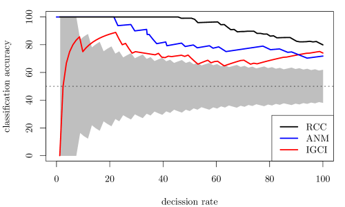
Figure 1: Accuracy of RCC, IGCI and ANM on the 82 scalar Tübingen pairs, as a function of decision rate. The grey area depicts accuracies not statistically significant.

Next, for each pair $(S_{i},l_{i})$, a new pair $(\{(y_{ij},x_{ij})\}_{j=1}^{n},-l_{i})$ is generated and added to $\mathcal{D}$. Finally, we train a random forest of $500$ decision trees with a minimum of $1\%$ of samples per leaf on the featurizations (5) of the dataset $\mathcal{D}$. We choose to use a random forest in this experiment because we are interested in reducing the variance of our predictions, since we are certain that the test data will not exactly follow the same distribution as our synthetic, training data. We evaluate the test classification accuracy of the random forest on the 82 one-dimensional Tübingen causal pairs (Peters et al., 2014; Zscheischler, 2014), which are curated from heterogeneous real-world data. Figure 1 plots the classification accuracy of RCC, IGCI and ANM versus the fraction of decisions that the algorithms are forced to make out of the 82 pairs. To compare these results to other lower-performance alternatives please refer to (Janzing et al., 2012). Overall, RCC shows the best performance, surpassing the state-of-the-art with a classification accuracy of $79\%$ when forced to infer the causal direction of all the 82 Tübingen pairs. The confidence of RCC is computed as the output probabilities of the random forest.

Note that our training data generating process is incredibly basic, and that a more powerful causal engine could be achieved by synthesising more heterogeneous causes, mapping mechanisms or noise distribution and pollution schemes. In a nutshell, RCC’s synthesising process should be guided by our prior knowledge about what kind of data we will typically have to analyze. This relates in spirit to the Bayesian causal inference strategy proposed by Stegle et al. (2010), but avoids the need of expensive, approximate inference at test time.

4.2 ChaLearn’s “Fast Causation Coefficient” challenge

The data of the ChaLearn’s Fast Causation Coefficient challenge (Guyon, 2014) consists on $20,000$ training pairs, $4,050$ validation pairs, and $4,050$ testing pairs. While the training data was available to the participants at all times during the competition, both validation and test sets were stored and predicted remotely on CodaLab’s servers.

According to the organizers, the challenge data was generated as follows. Each causal sample was drawn from the distribution of two random variables $X_{i}$ and $Y_{i}$, that can either be independent, related through a common unobserved cause, or causing each other. The data included both heterogeneous real-world (18% of the data) and artificial (82% of the data) causal pairs. The artificial data was generated using nonlinear models of the form $Y=f(X,\epsilon)$, $X=g(Y,\epsilon)$, and different noise combination strategies. The task of the participants was to use this data to derive a “causation coefficient” that would output “$+1$” whenever $X\rightarrow Y$, “-1” whenever $Y\rightarrow X$, and zero otherwise. The performance of each participant was measured using the “bidirectional AUC”, that is, the average of the Area Under the Curve (AUC) obtained on the two binary classification problems “$X\rightarrow Y$ vs all” and “$Y\rightarrow X$ vs all”.

Our strategy during the competition was as follows. First, we standardized each variable from each sample to have zero mean and unit variance. Second, we enlarged the dataset by duplicating each pair by swapping $X$ and $Y$ and its label accordingly. Third, we trained a Gradient Boosting Classifier (GBC), with hyper-parameters chosen via a 4-fold cross validation, on the featurizations (5) of the training data. In particular, we built two separate classifiers: a first one to distinguish between causal and non-causal pairs (i.e., $X-Y$ vs $\{X\rightarrow Y,X\leftarrow Y\}$), and a second one to distinguish between the two possible causal directions on the causal pairs (i.e., $X\rightarrow Y$ vs $X\leftarrow Y$). The final causation coefficient for a given sample $S_{i}$ was computed as

$$\mathrm{score}(S_{i})=p_{1}(S_{i})\cdot(2\cdot p_{2}(S_{i})-1),$$

where $p_{1}(x)$ and $p_{2}(x)$ are the class probabilities output by the first and the second GBCs, respectively. We found it easier to distinguish between causal and non-causal pairs than to infer the correct direction on the causal pairs.

RCC ranked third in the ChaLearn’s “Fast Causation Coefficient Challenge” competition, and was awarded the prize to the fastest running code (Guyon, 2014). At the time of the competition, we obtained a bidirectional AUC of $0.732843$ on the test pairs in two minutes of test-time Guyon (2014). On the other hand, the winning entry of the competition made use of hand-engineered features, took a test-time of 30 minutes, and achieved a bidirectional AUC of $0.826413$. However, some of the hand-engineered features used by this winning entry are of dubious importance for causal inference, but probably improved its score because of the existence of biases in the challenge data. Examples of these features are “unique number of samples from $X$”, “variance of $Y$” or “maximum value of $X$”.

Interestingly, the performance of IGCI on the $20,000$ training pairs is barely better than random guessing. The computational complexity of the additive noise model (usually implemented as two Gaussian Process regressions followed by two kernel-based independence tests) made it unfeasible to compare it on this dataset.

5 Conclusions and future Work

We have proposed to learn how to perform causal inference between pairs of random variables from observational data, by posing the task as as a supervised learning problem. In particular, we have introduced an effective and efficient featurization of probability distributions, based on kernel mean embeddings and random Fourier features. Our numerical simulations support the conjecture that patterns revealing causal relationships can be learnt from data.

We would like to mention three exciting research directions. First, the use of the hereby proposed ideas to learn other randomized statistics, such as measures of dependence (Lopez-Paz et al., 2013). Second, the extension of RCC to operate not on pairs, but sets of random variables, and eventually reconstruct causal DAGs from multivariate data. Finally, the adaption of the distributional learning theory of Szabó et al. (2014) to analyze our randomized, classification setting.

References

- Berlinet and Thomas-Agnan (2004) A. Berlinet and C. Thomas-Agnan. Reproducing Kernel Hilbert Spaces in Probability and Statistics. Kluwer Academic Publishers, 2004.
- Cartwright (1989) N. Cartwright. Nature’s Capacities and Their Measurement. Oxford Uni. Press, 1989.
- Daniusis et al. (2012) P. Daniusis, D. Janzing, J. Mooij, J. Zscheischler, B. Steudel, K. Zhang, and B. Schölkopf. Inferring deterministic causal relations. UAI, 2012.
- Guyon (2014) I. Guyon. Chalearn fast causation coefficient challenge, 2014. URL https://www.codalab.org/competitions/1381.
- Hoyer et al. (2009) P. O. Hoyer, D. Janzing, J. M. Mooij, J. R. Peters, and B. Schölkopf. Nonlinear causal discovery with additive noise models. NIPS, 2009.
- Janzing et al. (2012) D. Janzing, J. Mooij, K. Zhang, J. Lemeire, J. Zscheischler, P. Daniušis, B. Steudel, and B. Schölkopf. Information-geometric approach to inferring causal directions. Artificial Intelligence, 2012.
- Janzing et al. (2014) D. Janzing, B. Steudel, N. Shajarisales, and B. Schölkopf. Justifying information-geometric causal inference. arXiv, 2014.
- Kpotufe et al. (2013) S. Kpotufe, E. Sgouritsa, D. Janzing, and B. Schölkopf. Consistency of causal inference under the additive noise model. ICML, 2013.
- Lopez-Paz et al. (2013) D. Lopez-Paz, P. Hennig, and B. Schölkopf. The Randomized Dependence Coefficient. NIPS, 2013.
- Muandet et al. (2012) K. Muandet, K. Fukumizu, F. Dinuzzo, and B. Schölkopf. Learning from distributions via support measure machines. NIPS, 2012.
- Muandet et al. (2014) K. Muandet, K. Fukumizu, B. Sriperumbudur, A. Gretton, and B. Schölkopf. Kernel mean estimation and Stein effect. ICML, 2014.
- Peters et al. (2014) J. Peters, Joris M. M., D. Janzing, and B. Schölkopf. Causal discovery with continuous additive noise models. JMLR, 2014.
- Rahimi and Recht (2007) A. Rahimi and B. Recht. Random features for large-scale kernel machines. NIPS, 2007.
- Reichenbach (1956) H. Reichenbach. The Direction of Time. Dover, 1956.
- Rudin (1962) W. Rudin. Fourier Analysis on Groups. Wiley, 1962.
- Smola et al. (2007) A. J. Smola, A. Gretton, L. Song, and B. Schölkopf. A Hilbert space embedding for distributions. In ALT. Springer-Verlag, 2007.
- Sriperumbudur et al. (2010) B. K. Sriperumbudur, A. Gretton, K. Fukumizu, B. Schölkopf, and G. Lanckriet. Hilbert space embeddings and metrics on probability measures. JMLR, 2010.
- Stegle et al. (2010) O. Stegle, D. Janzing, K. Zhang, J. M. Mooij, and B. Schölkopf. Probabilistic latent variable models for distinguishing between cause and effect. 2010.
- Szabó et al. (2014) Z. Szabó, A. Gretton, B. Póczos, and B. Sriperumbudur. Two-stage sampled learning theory on distributions. arXiv preprints, 2014.
- Zhang and Hyvärinen (2009) K. Zhang and A. Hyvärinen. On the identifiability of the post-nonlinear causal model. UAI, 2009.
- Zscheischler (2014) J. Zscheischler. Benchmark data set for causal discovery algorithms, v0.8, 2014. URL http://webdav.tuebingen.mpg.de/cause-effect/.