Abstract

We propose a holographic dual for (pseudo-)conformal cosmological scenario, with a scalar field that forms a moving domain wall in adS₅. The domain wall separates two vacua with unequal energy densities. Unlike in the existing construction, the 5d solution is regular in the relevant space-time domain.

It has been understood for some time that the (nearly) flat spectrum of scalar cosmological perturbations may be a consequence of conformal symmetry $SO(4,2)$ broken down to de Sitter $SO(4,1)$ in the early Universe [1, 2, 3]. This has lead to (pseudo-)conformal cosmological scenario which serves as an alternative to inflation. In general terms [4], the symmetry breaking pattern is realized when a scalar operator (or several operators) ${\cal O}$ of non-zero conformal weight $\Delta$ acquires the time-dependent expectation value

$$\langle{\cal O}\rangle=\frac{\mbox{const}}{(-t)^{\Delta}}\;,$$ (1)

where $t<0$ and the rolling regime is supposed to terminate at some finite negative $t$, cf. Ref. [5]. Other ingredients of the scenario are: (i) nearly flat space-time at the rolling stage (1), hence no primordial tensor perturbations; (ii) another scalar field of zero conformal weight, whose perturbations automatically have flat power spectrum at late times at the rolling stage; (iii) conversion of these field perturbations into adiabatic perturbations at some later epoch. Among potentially observable predictions of this scenario are statistical anisotropy of scalar perturbations [7, 8, 9] and non-Gaussianities of specific shapes [9, 10, 11]. These features are to large extent generic consequences of the symmetry breaking pattern [9] $SO(4,2)\to SO(4,1)$.

It is of interest to construct a holographic dual to the (pseudo-)conformal scenario. A construction of this sort has been proposed in Ref. [12]. It employed free massive scalar field evolving in adS₅ with metric (hereafter the adS radius is set equal to 1)

$$ds^{2}=\frac{1}{z^{2}}\left(\eta_{\mu\nu}dx^{\mu}dx^{\nu}-dz^{2}\right)\;.$$ (2)

In the probe scalar field approximation, the corresponding solution is, however, singular at the null surface $z=-t$; upon switching on 5d gravity, the solution develops a naked singularity along the surface $z/(-t)=\mbox{const}<1$. This feature does not look particularly desirable, so one is lead to search for non-singular constructions.

On the other hand, the (pseudo-)conformal scenario is naturally realized in a DBI theory [13] descending from the dynamics of a thin brane in adS₅ [14]. So, it is natural to merge the two constructions and consider a thick brane evolution in adS₅ as a candidate for the holographic dual to the (pseudo-)conformal Universe. This is precisely the purpose of this paper.

To this end, we adopt a bottom-up approach, and instead of constructing a concrete CFT, simply consider a 5d theory of a scalar field with action

$$S=\int~{}\sqrt{g}\left(\frac{1}{2}g^{AB}\partial_{A}\phi\partial_{B}\phi-V(\phi)\right)~{}dz~{}d^{d}x$$ (3)

We will work in the probe scalar field approximation throughout, so that the metric (2) is unperturbed. We would like this theory to correspond to a boundary CFT without explicit breaking of conformal invariance, but with unstable conformally invariant vacuum $\phi=0$. So, unlike in Refs. [15, 16, 17] we assume that the potential $V(\phi)$ has a local minimum at $\phi=0$ and that the field behavior near the adS boundary $z=0$ is

$$\phi(z,x)=z^{\Delta_{+}}\phi_{0}(x)$$ (4)

with $\Delta_{+}=\sqrt{m^{2}+4}+2$, where $m$ is the scalar field mass in the vacuum $\phi=0$, and $\phi_{0}$ is related to the expectation value of a CFT operator [18, 19],

$$\langle{\cal O}\rangle=2\sqrt{m^{2}+4}~{}\phi_{0}\;.$$ (5)

The property (4) implies that there is no explicit deformation of the boundary CFT, in contrast to Refs. [16, 17, 20], whereas we allow for spontaneous breaking of conformal symmetry. To avoid possible runaway behavior in 5d theory, the potential $V(\phi)$ is assumed to have a global minimum at $\phi=\phi_{+}\neq 0$. Finally, we assume that the curvature of the potential at its maximum is large enough,

$$|V^{\prime\prime}(\phi_{max})|>2\;,$$ (6)

so that the solution we are about to discuss does not get stuck at this maximum, see below. So, from our viewpoit the position of the maximum is not particularly significant.

We are now going to construct a solution in adS for which the expectation value of the operator ${\cal O}$ given by (5) has the form (1), i.e., $\langle{\cal O}\rangle\propto(-t)^{-\Delta_{+}}$. This is a domain wall separating the vacua $\phi=0$ and $\phi=\phi_{+}$, with the false vacuum $\phi=0$ to the left of it.

The symmetry breaking pattern $SO(4,2)\to SO(4,1)$ is obtained for a 5d solution of the form [12]

$$\phi=\phi\left(\frac{t}{z}\right)\;$$ (7)

with asymptotics

$$\phi(v)\to(-v)^{-\Delta_{+}}\;\;\;\;\mbox{as}\;\;\;v\to-\infty\;,$$ (8)

where

$$v=\frac{t}{z}\;.$$

We require that the solution is non-singular at strictly negative $t$, but not necessarily at $t\geq 0$, since by assumption the rolling behavior (1) terminates at some finite negative time. Formally, the “point” $t=0,z=0$ is special, since it is reached from different directions, i.e., at different values of $v$ and hence different values of $\phi$. This can be interpreted as the “point” at which the wall hits the adS boundary.

With the Ansatz (7), the field equation is

$$(v^{2}-1)\frac{d^{2}\phi}{dv^{2}}+5v\frac{d\phi}{dv}-\frac{\partial V}{\partial\phi}=0\;.$$ (9)

For a class of potentials $V(\phi)$ it does admit a domain wall solution which is non-singular at $v<0$. To see this, consider first the vicinity of a null surface $v=-1$; note that at this surface eq. (9) is singular (the second derivative term vanishes). For any value of $\phi_{*}\equiv\phi(v=-1)$, there exists a non-singular solution

$$\phi=\phi_{*}-\frac{1}{5}V^{\prime}(\phi_{*})\cdot(v+1)-\frac{1}{14}V^{\prime}(\phi_{*})\left[1-\frac{1}{5}V^{\prime\prime}(\phi_{*})\right]\cdot(v+1)^{2}+\dots$$ (10)

For $v<-1$, we change the variable, $v=-\cosh\rho$ (cf. Ref. [12]) and write eq. (9) in the following form

$$\frac{d^{2}\phi}{d\rho^{2}}+4\frac{\cosh\rho}{\sinh\rho}\cdot\frac{d\phi}{d\rho}-\frac{\partial V}{\partial\phi}=0\;.$$ (11)

This equation corresponds to a motion of a “particle” in the inverted potential $-V$ with “time”-dependent friction, from $\rho=0$ ($z=-t$) to $\rho\to\infty$ ($z\to 0$). Let $V_{0}(\phi)$ be an auxiliary potential, such that there exists a solution to

$$\frac{d^{2}\phi}{dy^{2}}+4\frac{d\phi}{dy}-\frac{\partial V_{0}}{\partial\phi}=0\;,$$ (12)

that starts at $y\to-\infty$ in the true vacuum $\phi=\phi_{+}$ and reaches the false vacuum $\phi=0$ at $y\to\infty$. Note that the necessary condition for the existence of such a solution is that $|V_{0}^{\prime\prime}|>2$ at the maximum of $V_{0}$, cf. eq. (6). Incidentally, this solution can be interpreted as a static domain wall $\phi(y)$, where $y=-\log z$. In our context, this would be a domain wall centered at $\rho\to\infty$, i.e., asymptotically close to the adS boundary, where eq. (11) reduces to eq. (12). Now, let the potential $V(\phi)$ be slightly deeper than $V_{0}$ in the true vacuum, see Fig. 1. Then, by continuity, there exists a value of $\phi_{*}<\phi_{+}$ such that the solution to eq. (11) starts at $\rho=0$ from $\phi=\phi_{*}$ (at zero velocity $d\phi/d\rho$, since $v=-1-O(\rho^{2})$, see eq. (10)) and approaches the false vacuum $\phi=0$ as $\rho\to\infty$: a solution starting very close to the top of $(-V)$ overshoots the true vacuum, while a solution that starts from small $\phi$ undershoots it. So, at least for potentials sufficiently close to $V_{0}$, there exists a domain wall which is non-singular in the region $z<-t$. It has the asymptotics (8).

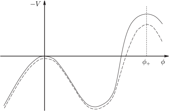
Figure 1: Inverted potential $[-V(\phi)]$ (solid line) and inverted auxiliary potential $[-V_{0}(\phi)]$ (dashed line).

Since the solution is non-singular at $z=-t$, it can be continued to the region $z>-t$. There, we change the variable to

$$v=-\cos\theta$$

and find from eq. (9)

$$\frac{d^{2}\phi}{d\theta^{2}}+4\frac{\cos\theta}{\sin\theta}\cdot\frac{d\phi}{d\theta}+\frac{\partial V}{\partial\phi}=0\;.$$ (13)

This corresponds to oscillations near $\phi=\phi_{+}$, which are damped at $\theta<\pi/2$, i.e., $t<0$. The fact that the potential is no longer inverted is easy to understand: normals to hypersurfaces $t/z=\mbox{const}$ are spacelike for $z<|t|$ and timelike for $z>|t|$.

Even though we are interested in the solution at $t<0$, we can pose a formal question of its behavior at positive $t$ ($\theta>\pi/2$). Clearly, the solution is non-singular at $\theta<\pi$, but generically develops a singularity at the null hypersurface $\theta=\pi$, i.e., $t=+z$. There is nothing wrong with that, since this null surface emanates from the special “point” $t=0$, $z=0$ where the wall hits the adS boundary.

We note in passing that by fine tuning the potential one can have solutions that are non-singular at $t=z$. Indeed, one can arrange the potential in such a way that the solution is symmetric under time reversal, $t\to-t$, i.e., $\theta\to\pi-\theta$. In that case, there exists also a domain wall at positive $t$ which expands to $z\to\infty$ as $t\to+\infty$. Whether such solutions with fine tuned potentials make sense from the CFT point of view remains to be understood.

To conclude, the (pseudo-)conformal scenario can be holographically implemented in a theory of 5d scalar field whose potential has both true and false vacua. In the 5d language, conformal rolling corresponds to a spatially homogeneous transition from the false vacuum to the true one, with a moving domain wall in between. We have demonstrated this within the probe scalar field approximation, but since the solution is non-singular in the relevant space-time domain, switching on gravity should not change the picture, at least in the weak gravity regime.

S.S. thanks Riccardo Rattazzi for useful discussions. The work of M.L. and V.R. has been supported by Russian Science Foundation grant 14-12-01430.

References

- [1] V. A. Rubakov, JCAP 0909 (2009) 030 [arXiv:0906.3693 [hep-th]].
- [2] P. Creminelli, A. Nicolis and E. Trincherini, JCAP 1011 (2010) 021 [arXiv:1007.0027 [hep-th]].
- [3] K. Hinterbichler and J. Khoury, JCAP 1204 (2012) 023 [arXiv:1106.1428 [hep-th]].
- [4] K. Hinterbichler, A. Joyce and J. Khoury, JCAP 1206 (2012) 043 [arXiv:1202.6056 [hep-th]].
- [5] Y. Wang and R. Brandenberger, JCAP 1210 (2012) 021 [arXiv:1206.4309 [hep-th]].
- [6] M. Osipov and V. Rubakov, JETP Lett. 93 (2011) 52 [arXiv:1007.3417 [hep-th]].
- [7] M. Libanov and V. Rubakov, JCAP 1011 (2010) 045 [arXiv:1007.4949 [hep-th]].
- [8] M. Libanov, S. Ramazanov and V. Rubakov, JCAP 1106 (2011) 010 [arXiv:1102.1390 [hep-th]].
- [9] P. Creminelli, A. Joyce, J. Khoury and M. Simonovic, JCAP 1304 (2013) 020 [arXiv:1212.3329].
- [10] M. Libanov, S. Mironov and V. Rubakov, Phys. Rev. D 84 (2011) 083502 [arXiv:1105.6230 [astro-ph.CO]].
- [11] S. A. Mironov, S. R. Ramazanov and V. A. Rubakov, JCAP 1404 (2014) 015 [arXiv:1312.7808 [astro-ph.CO]].
- [12] K. Hinterbichler, J. Stokes and M. Trodden, “Holography for a Non-Inflationary Early Universe,” arXiv:1408.1955 [hep-th].
- [13] K. Hinterbichler, A. Joyce, J. Khoury and G. E. J. Miller, JCAP 1212 (2012) 030 [arXiv:1209.5742 [hep-th]].
- [14] G. Goon, K. Hinterbichler and M. Trodden, JCAP 1107 (2011) 017 [arXiv:1103.5745 [hep-th]].
- [15] J. Distler and F. Zamora, Adv. Theor. Math. Phys. 2 (1999) 1405 [hep-th/9810206].
- [16] T. Hertog and G. T. Horowitz, JHEP 0407 (2004) 073 [hep-th/0406134].
- [17] T. Hertog and G. T. Horowitz, JHEP 0504 (2005) 005 [hep-th/0503071].
- [18] V. Balasubramanian, P. Kraus, A. E. Lawrence and S. P. Trivedi, Phys. Rev. D 59 (1999) 104021 [hep-th/9808017].
- [19] I. R. Klebanov and E. Witten, Nucl. Phys. B 556 (1999) 89 [hep-th/9905104].
- [20] B. Craps, T. Hertog and N. Turok, Phys. Rev. D 86 (2012) 043513 [arXiv:0712.4180 [hep-th]].