Characterizing short-term stability for Boolean networks over any distribution of transfer functions

Abstract

We present a characterization of short-term stability of random Boolean networks under arbitrary distributions of transfer functions. Given any distribution of transfer functions for a random Boolean network, we present a formula that decides whether short-term chaos (damage spreading) will happen. We provide a formal proof for this formula, and empirically show that its predictions are accurate. Previous work only works for special cases of balanced families. It has been observed that these characterizations fail for unbalanced families, yet such families are widespread in real biological networks.

I Introduction

Living systems composed of a wide variety of cells, genes, or organs operate with uncanny synchrony and stability, as do numerous engineered and social systems. In a series of seminal papers, Kauffman introduced Boolean networks to study such systems: this abstraction involves a network representing connectivity, and a family of Boolean functions determining states of network nodes to model dynamic behavior Kauffman69 ; Kauffman74 . Boolean networks have been used to model numerous dynamical systems, including genetic regulatory networks Kauffman69 and political systems Aldana03b , and have received much theoretical attention Harris02 ; Shmulevich04 ; Moreira05 ; Aldana03 ; Kauffman03 ; Shmulevich03 ; Mozeika11 ; Seshadhri11 ; Squires12 .

A Boolean network has a set of $n$ nodes linked to each other by a directed graph $G$. Each node $i$ has a Boolean state in $\{-1,+1\}$, an in-degree $K_{i}$, and an associated Boolean function $f_{i}:\{-1,+1\}^{K_{i}}\rightarrow\{-1,+1\}$, termed transfer function. If the state of node $i$ at time $t$ is $x_{i}(t)$, its state at time $t+1$ is described by $x_{i}(t+1)=f_{i}(x_{i_{1}}(t),\ldots,x_{i_{K_{i}}}(t)).$ For the sake of analysis, it is common to study a randomized ensemble of Boolean networks. The graph $G$ is a directed Erdős-Rényi network, where each each vertex $i$ chooses $K_{i}$ in-neighbors uniformly at random. There is an underlying distribution (or family) of Boolean transfer functions ${\cal F}$. Each vertex $i$ independently chooses the transfer function $f_{i}$ from ${\cal F}$.

A key parameter of interest is the short-term stability of the Boolean network. Specifically, if a single node has its state flipped, does the effect of this perturbation die out (quiescence), exponentially cascade over time (chaos), or is the system right in between (criticality)? There have been numerous empirical and mathematical observations about the characteristics of critical transition points in classes of Boolean networks Harris02 ; Shmulevich04 ; Moreira05 ; Aldana03 ; Kauffman03 ; Shmulevich03 ; Kesseli05 ; MoSaRa09 ; MoSaRa10 ; Seshadhri11 ; Squires12 , These results require ${\cal F}$ to have specific properties: for example, each truth table entry is i.i.d. or that functions are balanced (number of $+1$ and $-1$ outcomes is the same) on average.

These are severe restrictions. Various classes of functions occur naturally in biological and social applications, but do not satisfy either of these conditions. For example, Kauffman proposed a family of canalyzing functions Kauffman74 . A canalyzing function has at least one input, and one value of that input, that fully determines the output of the function. Kauffman observed that many elements of genetic regulatory systems have like nested canalyzing functions Kauffman74 ; Harris02 ; Kauffman03 ; Kauffman04 . Previous formal analyses do not yield precise characterizations of short-term stability for such families.

Threshold functions also occur in understanding processes on social and biological networks Sc78 ; Gr78 ; KeKlTa03 ; LiLo04 ; DaBo08 ; ZaAl11 ; TrMc13 A threshold function is of the form $f(x_{1},x_{2},\ldots,x_{K})=\mbox{sign}(\sum_{i}c_{i}x_{i}-\Theta)$, where $c_{i}$s and $\Theta$ are constants. Often there is a bias towards a particular state, so these previous characterizations fail to predict the critical threshold Seshadhri11 .

Our main result gives an exact formula for predicting the short-term dynamics of Boolean networks, for any distribution of transfer functions. We stress that our results are for ‘semi-annealed’ setting. Once we choose the topology of the Boolean network and the transfer functions from the appropriate distribution, we assume it is fixed. (We do not change these for each time-step, as in an annealed approximation.) All we need from the topology is a local tree-structure (as proved in Seshadhri11 and subsequently used in Squires12 ), which is guaranteed with high probability for Erdős-Rényi random graph distributions.

While no previous result provides such a formula, our work is closely related to the following. Mozeika and Saad MoSaRa09 ; MoSaRa10 ; Mozeika11 give a powerful generating function framework for analysis of Boolean networks, but do not characterize short-term stability. Seshadhri et al. Seshadhri11 introduced the notion of influence $\mathrm{I}({\cal F})$ of transfer function distribution ${\cal F}$, an easily computable quantity that determines the short-term behavior for a highly restricted class of balanced families ${\cal F}$: on average, functions in ${\cal F}$ are equally likely to output $+1$ and $-1$.

II Preliminaries

We are interested in the sensitivity of a Boolean network state $x(t)=\{x_{1}(t)\ldots,x_{n}(t)\}$ to a small initial perturbation. Formally, consider the following experiment. Suppose that a Boolean network starts from state $x$, and after $t$ steps reaches a state $F_{t}(x)$. Now, consider another initial state, $x^{(i)}$ which only differs from $x$ in the $i$th bit. Let $H_{t}$ be the expected Hamming distance between $F_{t}(x)$ and $F_{t}(x^{(i)})$, where $x$ is drawn from some specified (typically uniform) distribution. How does $H_{t}$ evolve with time? If $H_{t}$ can be expressed as $e^{\lambda t}$, then $\lambda$ is the Lyapunov exponent. If $\lambda<0$, the boolean network is quiescent; if $\lambda>0$, the network is chaotic.

We provide some notation and definitions.

• Biased distributions: We use ${\cal D}_{\rho}$ to denote the distribution over $\{-1,+1\}$ where the probability of $1$ is $(1+\rho)/2$. We choose this notation because the expected value is exactly $\rho$, the bias. Abusing notation, for $y\in\{-1,+1\}^{K}$, we say $y\sim{\cal D}_{\rho}$ when each coordinate of $y$ is chosen i.i.d. from ${\cal D}_{\rho}$.

• Imbalance: The imbalance of the Boolean network at time $t$, denoted by $\delta_{t}$, is $\sum_{i=1}^{n}x_{i}(t)/n$. Informally, this measures the difference between the $+1$s and $-1$s in the network. Observe that if the starting state $x(0)$ is chosen from ${\cal D}_{\rho}$, then $\delta_{0}=\rho$.

We use tools from harmonic analysis of Boolean functions, pioneered by Kahn, Kalai, and Linial Kahn88 . The convention in this field is that $-1$ denotes TRUE and $+1$ is FALSE (so multiplication in $\{-1,+1\}$ maps to XOR of $\{0,1\}$ bits). Consider $f:\{-1,+1\}^{K}\rightarrow\{-1,+1\}$, where we think of $f$ as one of the transfer functions. The standard representation is as a truth table, with $2^{K}$ entries in $\{-1,+1\}$. An alternative representation is as a linear combination of basis functions. In the following, we use $y\in\{-1,+1\}^{K}$ to denote an input to the transfer function. We use $[K]$ for set $\{1,2,\ldots,K\}$, which denotes the input coordinates. Refer to OD14 for details on the following.

• Parity functions: For any subset $S$ of coordinates in $[K]$, $\prod_{i\in S}y_{i}$ is the parity on $S$. (For $S=\emptyset$, we set the parity to be $1$.)

• Fourier representation: Any Boolean function $f$ can be expressed as $f(y)=\sum_{S\subseteq[K]}\widehat{f}(S)\prod_{i\in S}y_{i}$, where $\widehat{f}(S)$ are called Fourier coefficients. This expansion represents $f$ as a multilinear polynomial over the Boolean variables $y_{1},\ldots,y_{K}$. It can be shown that $\widehat{f}(S)=2^{-K}\sum_{y}f(y)\prod_{i\in S}y_{i}$, the correlation between $f$ and the parity on $S$. (The Fourier coefficients are the Walsh-Hadamard transform of the truth table.) There are exactly $2^{K}$ different Fourier coefficients, one for each subset of the $K$ inputs. For example, consider $K=2$, and the $AND$ function. A calculation yields $AND(y_{1},y_{2})=1/2+y_{1}/2+y_{2}/2-y_{1}y_{2}/2$.

• Level sets of coefficients, $\sigma_{r}$: Of special interest is $\sigma_{r}(f)=\sum_{C:|C|=r}\widehat{f}(C)$, where $0\leq r\leq K$. This is simply the sum of coefficients corresponding to sets of size $r$. Note that $\sigma_{0}(f)=\widehat{f}(\emptyset)$ $=\sum_{y}f(y)$. This is exactly the imbalance in the truth table of $f$.

• Influence: For any function $f$, the influence of the $i$th variable is denoted ${\rm{Inf}}_{i}(f)={\rm Pr}_{y}[f(y)\neq f(y^{(i)})]$ (where the probability is over the uniform distribution and $y^{(i)}$ is obtained by flipping $y$ at the $i$th bit), and the total influence is $\mathrm{I}(f)=\sum_{i}{\rm{Inf}}_{i}(f)$. We will define a biased version of this quantity, ${\rm{Inf}}_{i}(f;\rho)={\rm Pr}_{y\in{\cal D}_{\rho}}[f(y)\neq f(y^{(i)})]$, and analogously $\mathrm{I}(f;\rho)=\sum_{i}{\rm{Inf}}_{i}(f;\rho)$.

III Mathematical results

The proofs of our mathematical results are quite involved, and therefore provided in the supplemental material. We can derive closed form expressions for the evolution of $\delta_{t}$ (the expected imbalance at time $t$) and $H_{t}$ (the expected Hamming distance at time $t$ after a single bit perturbation).

The evolution of $\delta_{t}$ ($t>0$) is determined by the level sets of coefficients of the transfer functions. We use $\sigma_{r}({\cal F})=\hbox{\bf E}_{f\sim{\cal F}}[\sigma_{r}(f)]$ and $\mathrm{I}({\cal F};\delta)=\hbox{\bf E}_{f\sim{\cal F}}[\mathrm{I}(f;\delta)]$.

Theorem 1

Let initial state $x(0)$ be chosen from ${\cal D}_{\rho}$ (so $\delta_{0}=\rho$). Then $\delta_{t}$ evolves according to the polynomial recurrence $\delta_{t+1}=\sum_{r\geq 0}\sigma_{r}({\cal F})\delta^{r}_{t}$.

An equivalent formulation of the recurrence has been derived by the generating function method in Mozeika and Saad Mozeika11 , though their approach is completely different (they do not show a connection with Fourier coefficients). Our approach proves a clean description of this recurrence, since $\sigma_{r}({\cal F})$ can be easily computed from ${\cal F}$.

Our main theorem shows how the damage caused by a bit perturbation spreads.

Theorem 2

Let $\delta_{0},\delta_{1},\ldots$ be as given by Theorem 1. For $t\leq(\log n)/K$, $H_{t}=\prod_{0\leq h<t}\mathrm{I}({\cal F};\delta_{h})$.

In many situations, $\delta_{t}$ converges to some $\delta^{*}$. In that case, $H_{t}\approx[\mathrm{I}({\cal F};\delta^{*})]^{t}$. The Lyapunov exponent is $\log\mathrm{I}({\cal F};\delta^{*})$, so we get a critical point at $\mathrm{I}({\cal F};\delta^{*})=1$. Our formula gives a provable characterization of short-term stability, for any transfer function family ${\cal F}$.

Balanced families: As a warmup, we derive previous results that only held for balanced families ${\cal F}$. In such families, the expected difference (over ${\cal F}$) between $+1$’s and $-1$’s in the transfer functions is exactly zero. This contains the classic random families of Kauffman. For such a family, $\sigma_{0}({\cal F})=\hbox{\bf E}_{f\sim{\cal F}}[\sigma_{0}(f)]=0$. The starting distribution is given by ${\cal D}_{0}$, so $\delta_{0}=0$. Regardless of the values of $\sigma_{r}({\cal F})$ (for $r>0$), by Theorem 1, $\delta_{t}=0$ for all $t$. Hence, $H_{t}=[\mathrm{I}({\cal F};0)]^{t}$, and $\mathrm{I}({\cal F};0)=1$ is the critical threshold. This is exactly the main result of Seshadhri11 .

IV Applications

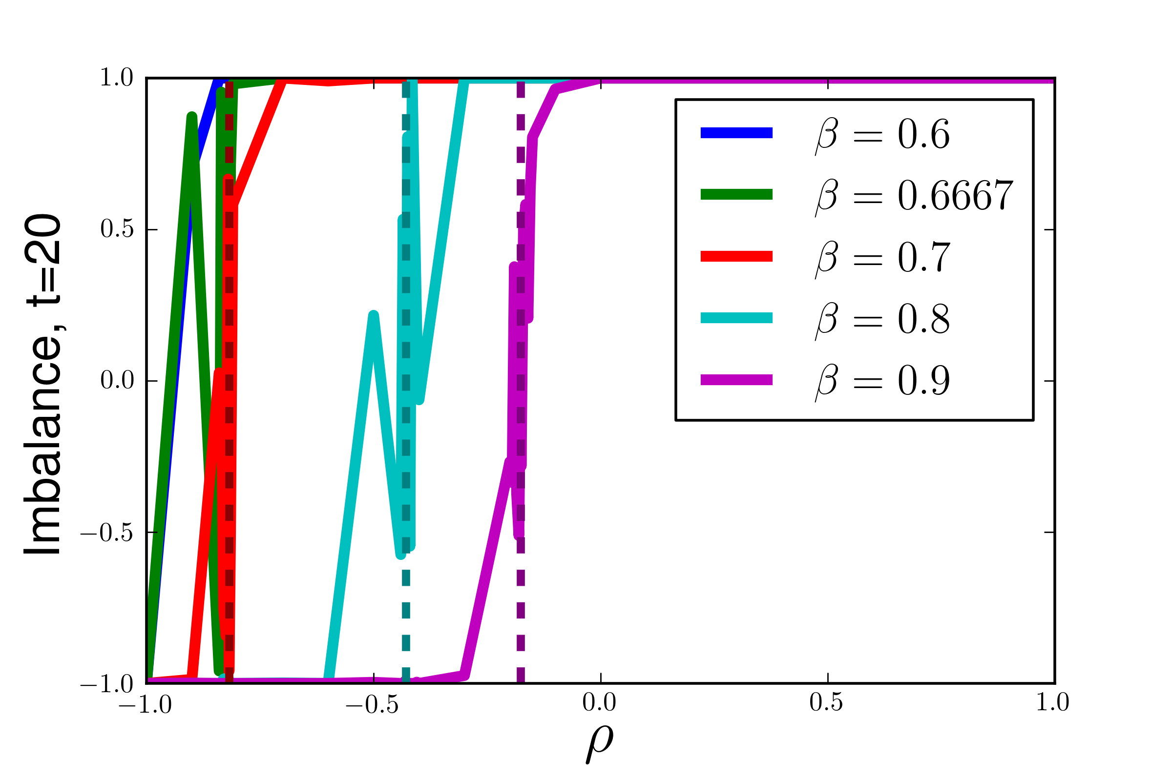
(a) Imbalance for different $\beta$ as $\rho$ increases for threshold function distribution

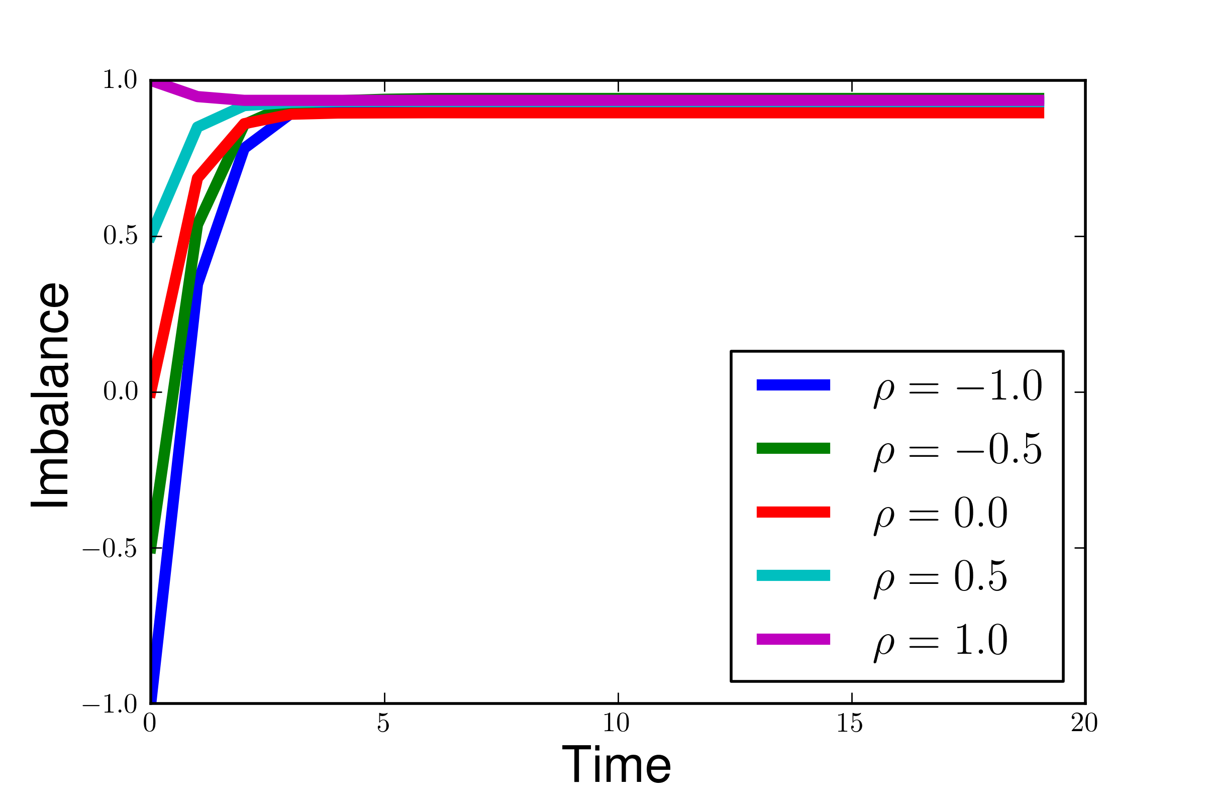
(b) Imbalance for different $\rho$ as time increases for nested canalyzing distribution

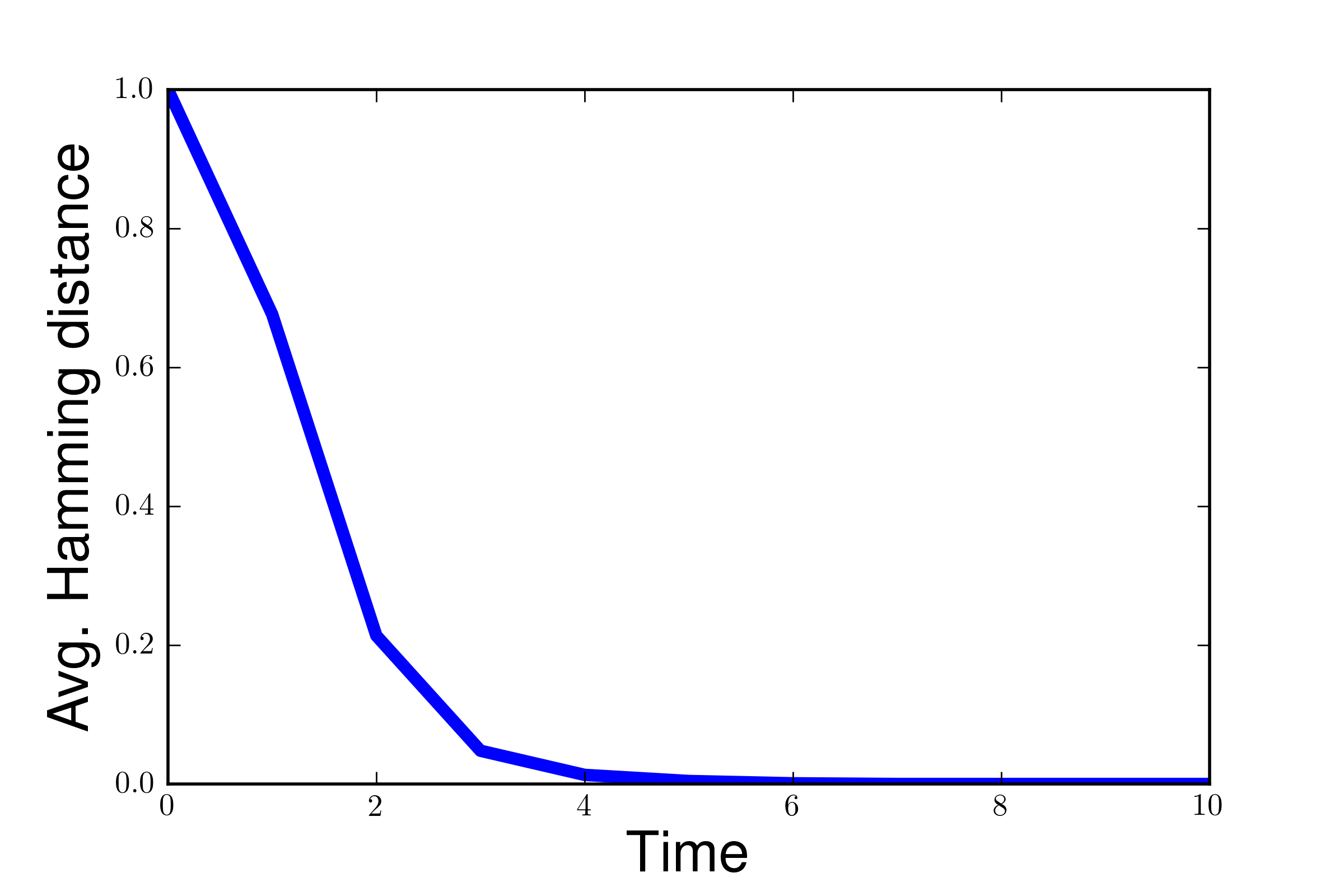
(c) Hamming distance as time increases for nested canalyzing distribution

Figure 1: Experimental results

Mixtures of threshold function families: Threshold functions are commonly used to understand the spread of new ideas/viral propogations in social networks, inspired by pioneering work in sociology Sc78 ; Gr78 ; KeKlTa03 . Think of two kinds of people (vertices) in a network. Some simply side with the majority of their neighbors. Others are more resistant to change, and only take up a new belief if all their neighbors believe it. We will first demonstrate our theorem on a synthetic distribution inspired by this application. For simplicity of analysis (and to see all the math), set $K=3$. The majority function is $MAJ(y)=\mbox{sign}(\sum_{i}y_{i})$ and the AND function $AND(y)=\mbox{sign}(\sum_{i}y_{i}+2.5)$ (this is $-1$ iff all inputs are $-1$). Our distribution ${\cal F}$ picks $MAJ$ with probability $\beta$ and $AND$ with probability $1-\beta$. How much of the initial network needs to have a new belief for it to propogate through the network? (And how is this sensitive to perturbation?) Formally, what is the dynamics for initial distribution ${\cal D}_{\rho}$? Think of a vertex state being $-1$ (TRUE) if that vertex currently believes the new idea. We start with the Fourier expansions of $MAJ$ and $AND$.

$$MAJ(y)=\sum_{i}y_{i}/2-y_{1}y_{2}y_{3}/2$$

$$AND(y)=3/4+\sum_{i}y_{i}/4-\sum_{i\neq j}y_{i}y_{j}/4+y_{1}y_{2}y_{3}/4$$

We compute $\sigma_{0}({\cal F})=3(1-\beta)/4$, $\sigma_{1}({\cal F})=3\beta/2+3(1-\beta)/4=3(1+\beta)/4$, $\sigma_{2}({\cal F})=3(\beta-1)/4$, and $\sigma_{3}({\cal F})=-\beta/2+(1-\beta)/4=(1-3\beta)/4$. From Theorem 1,

$$\delta_{t+1}=(1-3\beta)\delta^{3}_{t}/4 +3(\beta-1)\delta^{2}_{t}/4$$

$$+3(1+\beta)\delta_{t}/4+3(1-\beta)/4$$

Any fixed point is a root of the following polynomial $p(\delta)$ (which basically measures $\delta_{t+1}-\delta_{t}$). Note that when $p(\delta_{t})>0$, then $\delta_{t+1}>\delta_{t}$ (and vice versa).

$$p(\delta) =[(1-3\beta)\delta^{3}+3(\beta-1)\delta^{2}+(3\beta-1)\delta+3(1-\beta)]/4$$

$$=(\delta-1)(\delta+1)[(1-3\beta)\delta-3(1-\beta)]/4$$

This characterizes the limits of $\delta_{t}$ as $t\rightarrow\infty$ (assuming convergence). The first two are trivial roots, since the all $-1$s and all $+1$s states are fixed points imbalances for the Boolean network. The third root $3(1-\beta)/(1-3\beta)$ is a new valid imbalance (in the range $(-1,1)$) only when $\beta>2/3$.

Now, we can explain the dynamics. (We ignore the trivial cases $\rho=-1,+1$.)

• $\beta\leq 2/3$: The polynomial $p(z)>0$ for any $z\in(-1,1)$. Hence, for any non-trivial starting distribution ${\cal D}_{\rho}$, the Boolean network converges to the all $+1$s state. So the new belief will always die out.

• $\beta>2/3$: There exists a new unstable fixed point for the imbalance at $\delta^{*}=3(1-\beta)/(1-3\beta)$. We have $p(z)>0$ if $z>\delta^{*}$ and $p(z)<0$ if $z<\delta^{*}$. If $\rho>\delta^{*}$, the eventual state is all $+1$s. If $\rho<\delta^{*}$, the eventual state is all $-1$s.

To understand the sensitivity to bit flips, it is quite natural that for situations where $\delta_{t}$ converges to $-1$ or $+1$, the network is insensitive to perturbations. Calculations yield that ${\rm{Inf}}({\cal F};-1)$ and ${\rm{Inf}}({\cal F};+1)$ are $<1$. By Theorem 2, the networks are quiescent. At $\rho=\delta^{*}$, $\mathrm{I}({\cal F};\delta^{*})=3\beta(1-(\delta^{*})^{2})/2+3(1-\beta)(1-\delta^{*})^{2}/4$. By some elementary algebra, $\mathrm{I}({\cal F};\delta^{*})>1$ when $\beta>2/3$. Hence, for $\rho=\delta^{*}$, the dynamics are chaotic (again, this is expected).

We performed simulations on Boolean networks with $10^{4}$ nodes. For a given $\beta$, we vary the starting distribution $\rho$ and measure the imbalances at $t=20$. (This was averaged over 1000 runs.) The results are in Figure 1a, where each colored line denotes a different choice of $\beta$. The predicted transition of $\delta^{*}=3(1-\beta)/(1-3\beta)$ is denoted by the dashed line, coinciding nicely with the experimental transition point. As expected we see some fluctations (due to chaotic behavior at $\delta^{*}$) at the transition point.

Nested canalyzing functions: For a real application, we consider the nested canalyzing functions of Kauffman04 . (We provide a full description of this distribution in the supplement.) Previous work suggests that this distribution is reflective of real biological networks and is quiescent. We can use our theorems to validate the quiescence. Let us the consider the polynomial $\delta_{t+1}-\delta_{t}$. For example at $K=5$, a technical calculation yields $p(\delta)=-0.001\delta^{4}+0.016\delta^{3}-0.11\delta^{2}-0.69\delta+0.71$. For $K=10$, $p(\delta)=-0.007\delta^{4}+0.012\delta^{2}-0.099\delta^{2}-0.7\delta+0.71$. These polynomials have a single stable root $\delta^{*}\approx 0.9$ in $[-1,+1]$. Even as $K$ varies, the root is quite stable, so that fixed point imbalance is at least $0.9$ regardless of the degree distribution.

We perform experiments for varying degree distributions with $10^{4}$ nodes, and varying starting state distributions ${\cal D}_{\rho}$. (We show only the results for $K=5$ for space reasons.) In Figure 1b, we plot the imbalance as a function of time for varying $\rho$. Observe that the imbalance always converges to around $0.9$. This means that roughly 90% of the nodes converge to the $+1$ (FALSE) state. The influence $\mathrm{I}({\cal F};\delta^{*})$ is roughly $0.3$, so the network is quiescent. This is validated by the Derrida plot in Figure 1c, which plots average Hamming distance over time (for $\rho=0$). We observe that the Hamming distance rapidly decays to $0$.

V Acknowledgements

Sandia is a multiprogram laboratory operated by Sandia Corporation, a wholly owned subsidiary of Lockheed Martin Corporation, for the U.S. Department of Energy under contract DE-AC04-94AL85000.

Supplemental Material

Appendix A Preliminaries and notation

For convenience, we state and formalize many of the basic concepts already introduced in the main body.

For $\rho\in[-1,1]$, we define a biased distribution ${\cal D}_{\rho}$ on ${\cal B}$ as follows. The probability of $+1$ is $(1+\rho)/2$ and that of $-1$ is $(1-\rho)/2$. Note that expectation is exactly $\rho$. We sometimes abuse notation and use ${\cal D}_{\rho}$ to denote the product distribution over $n$ bits. The uniform distribution is given by ${\cal D}_{0}$.

We assume that there is a distribution ${\cal T}$ on transfer functions. Formally, this is a union of distributions ${\cal T}_{d}$, where this family only contains boolean functions that take $d$ inputs. For each vertex $v$ with indegree $d$, we first choose an independent function $f_{v}(y_{1},y_{2},\ldots,y_{d})$ from ${\cal T}_{d}$. Randomly permute the in-neighbors of $i$ to get a list $v_{1},v_{2},\ldots,v_{d}$. Assign the vertex $v_{j}$ to input $y_{j}$ of $\phi_{i}$. This gives us the transfer function for vertex $i$.

A convenient method for ignoring varying degrees is the following. We assume that each vertex has an indegree of $K$, with neighbors chosen randomly as before. Any function $\phi$ with less than $d<K$ inputs can be extended to have $K$ inputs, where $\phi$ does not depend on the new $K-d$ inputs. We now apply the same construction, where there is a single distribution ${\cal T}$ over input functions.

For a boolean network ${\cal N}$, we use $f_{t}(x)$ to denote the total state after $t$ steps starting with an initial state $x$. We use $f_{v,t}(x)$ to denote the (boolean) state at the vertex $v$. Our aim is to understand $H_{t}=(1/n)\sum_{i=1}^{n}\hbox{\bf E}_{x\in{\cal D}_{\rho}}[f_{t}(x)-f_{t}(x^{(i)})]$. Meaning, we look at the expected Hamming distance over the starting state $x$ for a random bit flip. As proven in previous work, this is the same as $\frac{1}{n}\sum_{1\leq u,v\leq n}{{\rm{Inf}}_{u}}({f_{v,t}};{\rho})$. This is the average value (over all vertices $v$) of $\sum_{u}{{\rm{Inf}}_{u}}({f_{v,t}};{\rho})$. Since the construction of boolean networks is random where all vertices are symmetric, in expectation, all these influence sums are the same. Hence, we will fix a single vertex and focus on this sum.

Appendix B Fourier Analysis of Boolean Functions

We will focus on functions of the form $f:\{-1,+1\}^{K}\longrightarrow\{-1,+1\}$. We think of a function as a vector in $\mathbb{R}^{2^{K}}$, which is just an explicit representation of the truth table. The Fourier basis for Boolean functions (also called the Walsh-Hadamard basis) provides an alternate basis to represent functions.

Definition 3

• Let $S\subseteq[K]$. The parity on $S$ is the function $\chi_{S}(y)=\prod_{i\in S}y_{i}$. Conventionally, the function $\chi_{\emptyset}$ is a constant function that takes value $+1$.

• For $S\subseteq[K]$, define $\widehat{f}(S):=\hbox{\bf E}_{x\in{\cal D}_{0}}[f(y)\chi_{S}(y)]=2^{-K}\sum_{x}f(y)\chi_{S}(y)$.

The fundamental theorem is that the parities form an orthonormal basis for functions $f$ on the ${\cal B}^{d}$. This gives the Fourier expansion of $f$.

Theorem 4

Every function $f:\{-1,+1\}^{d}\longrightarrow\mathbb{R}$ is uniquely expressible as a linear combination of the parity functions. Formally, $f=\sum_{S\subseteq[K]}\widehat{f}(S)\chi_{S}$.

The influences are fundamentally connected to the Fourier expansion.

Proposition 5

The value of ${{\rm{Inf}}_{i}}({f};{\rho})$ is equal to the following three expressions.

• $(1/4)\hbox{\bf E}_{x\sim{\cal D}_{\rho}}[(f(y)-f(y^{(i)}))^{2}]$

• $\hbox{\bf E}_{x\sim{\cal D}_{\rho}}[\big{(}\sum_{S\ni i}\widehat{f}(S)\chi_{S\backslash i}(y)\big{)}^{2}]$

Proof: Since the probability distribution is always ${\cal D}_{\rho}$, we drop the subscript $x\sim{\cal D}_{\rho}$. We have ${{\rm{Inf}}_{i}}({f};{\rho})=\Pr[f(y)\neq f(y^{(i)})]$. Observe that $(f(y)-f(y^{(i)}))^{2}=4$ if $f(y)\neq f(y^{(i)})$ and zero otherwise. Hence, $4\cdot{{\rm{Inf}}_{i}}({f};{\rho})=\hbox{\bf E}[(f(y)-f(y^{(i)}))^{2}]$. We expand this expression.

$$4\cdot{{\rm{Inf}}_{i}}({f};{\rho})=\hbox{\bf E}[(f(y)-f(y^{(i)}))^{2}]$$

$$= \hbox{\bf E}[\Big{(}\sum_{S}\widehat{f}(S)(\prod_{j\in S}y_{j}-\prod_{j\in S}y^{(i)}_{j})\Big{)}^{2}]$$

$$= \hbox{\bf E}[\Big{(}\sum_{S\ni i}\widehat{f}(S)(y_{i}-y^{(i)}_{i})\prod_{j\in S\backslash i}y_{j}\Big{)}^{2}]\ \ \ \ \textrm{(since for $j\neq i$, $y_{j}=y^{(i)}_{j}$)}$$

$$= 4\hbox{\bf E}[\Big{(}\sum_{S\ni i}\widehat{f}(S)\prod_{j\in S\backslash i}y_{j}\Big{)}^{2}]\ \ \ \ \textrm{(since $|y_{i}-y^{(i)}_{i}|=2$)}$$

$\Box$

Appendix C Deriving the recurrences

Fix a vertex $v$. Let us consider the function $f_{v,t}$ for small $t\ll\log n$. Previous work tells us that we can assume (asymptotically) this is a rooted tree Seshadhri11 . We use $N^{-}_{\leq t,v}$ to denote the $t$-step in-neighborhood of vertex $i$.

Claim 6

Fix a vertex $v$ and let $t\leq(\log n)/(4K)$. The probability that the subgraph induced by $N^{-}_{\leq t,v}$ is a directed tree is at least $1-1/\sqrt{n}$.

The distribution ${\cal B}_{t}$: We define a distribution on Boolean networks that runs for $t$ steps on rooted trees with height $t$. This captures the $t$-neighborhood of $v$ based on Claim 6. We take a $K$-ary directed tree rooted at $v$ of depth $t$ , with edges pointing towards the root $v$. For every internal node $u$, we choose a transfer function $\phi_{u}$ distributed according to ${\cal F}$. The leaves of the tree are the input nodes, collectively denoted as $x$. We will set the state at leaf nodes from the distribution ${\cal D}_{\rho}$. So $\delta_{0}=\rho$ is the initial imbalance.

The Boolean network runs for $t$ steps to yield the state at the root. Observe that for a vertex $u$ at height $h$, only the function $f_{u,h}$ is defined.

We will use $v_{1},v_{2},\ldots$ to denote the children of $v$. The Fourier expansion yields the following claim. This innocuous statement is the heart of the analysis.

Claim 7

$f_{v,t}=\sum_{A\subseteq[K]}\widehat{\phi_{v}}(A)\prod_{i\in A}f_{v_{i},t-1}$

Proof: Suppose the state at $v_{i}$ is $y_{i}$. The state at $v$ is determined by applying the transfer function $\phi_{v}$ on the states $(y_{1},y_{2},\ldots,y_{K})$. Using the Fourier expansion of $\phi_{v}$, we get the state at $v$ is $\sum_{A\subseteq[K]}\widehat{\phi_{v}}(A)\prod_{i\in A}y_{i}$. The state $y_{i}$ is given by the function $f_{v_{i},t-1}$, and the state at $v$ is $f_{v,t}$. $\Box$

C.1 The imbalance recurrence

We derive a polynomial recurrence for $\delta_{t}$, the expected imbalance at a vertex after $t$ steps. We have $\delta_{t}=\hbox{\bf E}_{{\cal B}_{t}}[\hbox{\bf E}_{x\in{\cal D}_{\rho}}[f_{v,t}(x)]]$. For any $r$, remember that $\sigma_{r}=\hbox{\bf E}_{\phi\sim{\cal F}}[\sum_{C:|C|=r}\widehat{\phi}(C)]$.

Theorem 8

Let $\delta_{t}$ be the expected imbalance at time $t$. For $t\geq 1$, $\delta_{t}$ evolves according to the following iterated polynomial map.

$$\delta_{t}=\sum_{r\geq 0}\sigma_{r}\delta^{r}_{t-1}$$ (1)

Proof: We take expectations of the formula in Claim 7. (Verbal explanation follows.)

$$\delta_{t}=\hbox{\bf E}_{x,{\cal B}_{t}}[f_{v,t}(y)] = \hbox{\bf E}_{x,{\cal B}_{t}}[\sum_{A\subseteq[K]}\widehat{\phi_{v}}(A)\prod_{i\in A}f_{v_{i},t-1}(y)]$$

$$= \sum_{A\subseteq[K]}\hbox{\bf E}_{x,{\cal B}_{t}}\Big{[}\widehat{\phi_{v}}(A)\prod_{i\in A}f_{v_{i},t-1}(y)\Big{]}$$

$$= \sum_{A\subseteq[K]}\hbox{\bf E}_{{\cal F}}[\widehat{\phi}(A)]\prod_{i\in A}\hbox{\bf E}_{x,{\cal B}_{t-1}}[f_{v_{i},t-1}(y)]$$

The second line is just linearity of expectation. The final line is obtained through independence. Note that $\phi_{v}$ is independent of the Boolean networks rooted at the $v_{i}$s. These Boolean networks are also independent of each other. Hence, the expectation of the product is the product of expectations. The function $\phi_{v}$ is a random function $\phi$ chosen from ${\cal F}$. Because of the recursive construction, the distribution of ${\cal B}_{t}$ rooted at $v$ induces the distribution of ${\cal B}_{t-1}$ rooted at the $v_{i}$s. Now, observe that $\hbox{\bf E}_{x,{\cal B}_{t-1}}[f_{v_{i},t-1}(y)]=\delta_{t-1}$.

Plugging this in and collecting all terms corresponding to sets of the same size,

$$\delta_{t} = \sum_{A\subseteq[K]}\delta^{|A|}_{t-1}\hbox{\bf E}_{{\cal F}}[\widehat{\phi}(A)]$$

$$= \sum_{r\geq 0}\delta^{r}_{t-1}\sum_{A:|A|=r}\hbox{\bf E}_{\cal F}[\widehat{\phi}(A)]=\sum_{r\geq 0}\sigma_{r}\delta^{r}_{t-1}$$

$\Box$

C.2 The spreading of perturbations

We focus on $\mathrm{I}_{t}(\rho_{0})$, the expected average (over all nodes) influence of a node at $t$-steps, when the initial distribution is ${\cal D}_{\rho_{0}}$. By the tree approximation, it suffices to focus on the node $v$ and consider the distribution ${\cal B}_{t}$. We can express $\mathrm{I}_{t}(\rho_{0})$ as follows.

By the tree approximation, $H_{t}=\hbox{\bf E}_{{\cal B}_{t}}[\sum_{\ell}{\rm{Inf}}_{\ell}(f_{v,t});\rho]$ (where $\ell$ is over all leaves). In words, we look at the $\rho$-biased influence summed over all leaves. For convenience, we will drop the time/height subscript and simply write $f_{u}$ instead of $f_{u,h}$.

Theorem 9

$H_{t}=\prod_{0\leq h<t}{\mathrm{I}({\cal F};{{\delta_{h}}})}$

Proof: Partition the leaves into subsets $S_{1},S_{2},\ldots,S_{K}$, where $S_{i}$ contains all leaves that are descendants of $v_{i}$. Focus on a leaf $\ell\in S_{1}$. By Prop. 5 and Claim 7,

$$\hbox{\bf E}_{{\cal B}_{t}}[{\rm{Inf}}_{\ell}(f_{v};\rho)]$$

$$= (1/4)\hbox{\bf E}_{{\cal B}_{t},x\sim{\cal D}_{\rho}}[(f_{v}(x)-f_{v}(x^{(\ell)}))^{2}]$$

$$= (1/4)\hbox{\bf E}_{{\cal B}_{t},x\sim{\cal D}_{\rho}}[\Big{\{}\sum_{A}\widehat{\phi}_{v}(A)(\prod_{i\in A}f_{v_{i}}(x)-\prod_{i\in A}f_{v_{i}}(x^{(\ell)}))\Big{\}}^{2}]$$

Observe that for $i\neq 1$, $f_{v_{i}}(x)=f_{v_{i}}(x^{(\ell)})$. (This is because $\ell$ is not in the subtree of $v_{i}$.) In the summation above, only the terms corresponding to $A\ni 1$ are non-zero. Expanding further,

$$\big{\{}\sum_{A\ni 1}\widehat{\phi}_{v}(A)(\prod_{i\in A}f_{v_{i}}(x)-\prod_{i\in A}f_{v_{i}}(x^{(\ell)}))\big{\}}^{2}$$

$$= \Big{\{}\sum_{A\ni 1}\widehat{\phi}_{v}(A)\big{(}\prod_{\begin{subarray}{c}i\in A\\ i\neq 1\end{subarray}}f_{v_{i}}(x)\big{)}(f_{v_{1}}(x)-f_{v_{1}}(x^{(\ell)}))\Big{\}}^{2}$$

$$= \big{(}f_{v_{1}}(x)-f_{v_{1}}(x^{(\ell)})\big{)}^{2}\Big{\{}\sum_{A\ni 1}\widehat{\phi}_{v}(A)\prod_{\begin{subarray}{c}i\in A\\ i\neq 1\end{subarray}}f_{v_{i}}(x)\Big{\}}^{2}$$

Each $f_{v_{i}}$ is defined over disjoint parts of the underlying tree with disjoint inputs. Hence, when we take the expectation $\hbox{\bf E}_{{\cal B}_{t},x}$ over the product, we get the product of expectations. Moreover, $(1/4)\hbox{\bf E}_{{\cal B}_{t},x\sim{\cal D}_{\rho}}[\big{(}f_{v_{1}}(x)-f_{v_{1}}(x^{(\ell)})\big{)}^{2}]$ is exactly $\hbox{\bf E}_{{\cal B}_{t-1}}[{{\rm{Inf}}_{\ell}}({f_{v_{1}}};{\rho})]$.

The random variable $f_{v_{i}}(x)$ is in $\{-1,+1\}$ and $\hbox{\bf E}_{{\cal B}_{t-1},x\sim{\cal D}_{\rho}}[f_{v_{i}}(x)]=\delta_{t-1}$. Hence, it is distributed as ${\cal D}_{\delta_{t-1}}$. Taking expectations over ${\cal B}_{t-1},x$, setting $y_{i}=f_{v_{i}}(x)$ and Prop. 5,

$$\hbox{\bf E}_{{\cal B}_{t},x\sim{\cal D}_{\rho}}[\big{\{}\sum_{A\ni 1}\widehat{\phi}_{v}(A)\prod_{\begin{subarray}{c}i\in A\\ i\neq 1\end{subarray}}f_{v_{i}}(x)\big{\}}^{2}]$$

$$= \hbox{\bf E}_{\phi\sim{\cal F},y\sim{\cal D}_{\delta_{t-1}}}[\big{\{}\sum_{A\ni 1}\widehat{\phi}_{v}(A)\prod_{\begin{subarray}{c}i\in A\setminus 1\end{subarray}}y_{i}\big{\}}^{2}]$$

$$= \hbox{\bf E}_{\phi\sim{\cal F}}[{{\rm{Inf}}_{1}}({\phi};{\delta_{t-1}})]$$

In general, for $\ell\in S_{i}$, we get $\hbox{\bf E}_{{\cal B}_{t}}[{\rm{Inf}}_{\ell}(f_{v};\rho)]=\hbox{\bf E}_{\cal F}[{{\rm{Inf}}_{i}}({\phi};{\delta_{t-1}})]\hbox{\bf E}_{{\cal B}_{t-1}}[{{\rm{Inf}}_{\ell}}({f_{v_{i}}};{\rho})]$. We combine all our observations.

$$H_{t} = \sum_{\ell}\hbox{\bf E}_{{\cal B}_{t}}[{\rm{Inf}}_{\ell}(f_{v,t};\rho)]$$

$$= \sum_{i=1}^{K}\sum_{\ell\in S_{i}}\hbox{\bf E}_{{\cal B}_{t}}[{\rm{Inf}}_{\ell}(f_{v,t})]$$

$$= \sum_{i=1}^{K}\hbox{\bf E}_{{\cal F}}[{{\rm{Inf}}_{i}}({\phi};{\delta_{t-1}})]\sum_{\ell\in S_{i}}\hbox{\bf E}_{{\cal B}_{t-1}}[{{\rm{Inf}}_{\ell}}({f_{v_{i}}};{\rho})]$$

$$= \sum_{i=1}^{K}\hbox{\bf E}_{{\cal F}}[{{\rm{Inf}}_{i}}({\phi};{\delta_{t-1}})]\hbox{\bf E}_{{\cal B}_{t-1}}[\sum_{\ell\in S_{i}}{{\rm{Inf}}_{\ell}}({f_{v_{i}}};{\rho})]$$

$$= H_{t-1}\sum_{i=1}^{K}\hbox{\bf E}_{{\cal F}}[{{\rm{Inf}}_{i}}({\phi};{\delta_{t-1}})]$$

$$= H_{t-1}\cdot{\mathrm{I}({\cal F};{\delta_{t-1}})}$$

Uncoiling the recurrence yields the theorem. $\Box$

Appendix D Nested canalyzing functions

For completeness, we describe this distribution. Fix positive integer $\alpha$ and a series of canalyzing input values $c_{1},c_{2},\ldots,c_{K}$ and $d_{1},d_{2},\ldots,d_{K},d_{def}$ (where each of these is in $\{-1,+1\}$). The function is defined as follows:

$$f(x)=\begin{cases}d_{1}&\text{if }y_{1}=d_{1}\\ d_{2}&\text{if }y_{1}\neq d_{1}\text{and }y_{2}=d_{2}\\ \vdots&\\ d_{K}&\text{if }y_{1}\neq d_{1},y_{2}\neq d_{2},\ldots,y_{K-1}\neq d_{K-1}\text{and }y_{K}=d_{k}\\ d_{def}&\text{otherwise}\end{cases}$$

For any parameter $\alpha>0$, the distribution is given by $\Pr[c_{i}=-1]=\Pr[d_{i}=-1]=\exp(-\alpha/2^{i})/(1+\exp(-\alpha/2^{i}))$. Kauffman et al suggest that $\alpha=7$ is reflective of real biological networks, and corresponding boolean networks are quiescent.

References

- (1) S. A. Kauffman, “Metabolic stability and epigenesis in randomly connected nets,” Journal of Theoretical Biology, vol. 22, no. 3, pp. 437–467, 1969.
- (2) S. A. Kauffman, “The large scale structure and dynamics of gene control circuits: An ensemble approach,” Journal of Theoretical Biology, vol. 44, no. 1, pp. 167–190, 1974.
- (3) M. Aldana, S. Coppersmith, and L. P. Kadanoff, “Boolean dynamics with random couplings,” in Perspectives and Problems in Nolinear Science (K. E, M. JE, and S. KR, eds.), pp. 23–89, Springer-Verlag, 2003.
- (4) S. E. Harris, B. K. Sawhill, A. Wuensche, and S. A. Kauffman, “A model of transcriptional regulatory networks based on biases in the observed regulation rules,” Complexity, vol. 7, no. 4, pp. 23–40, 2002.
- (5) I. Shmulevich and S. A. Kauffman, “Activities and sensitivities in bolean network models,” Physical Review Letters, vol. 93, no. 4, p. 048701, 2004.
- (6) A. A. Moreira and L. A. N. Amaral, “Canalizing kauffman networks: Nonergodicity and its effect on their critical behavior,” Physical Review Letters, vol. 94, p. 218702, 2005.
- (7) M. Aldana and P. Cluzel, “A natural class of robust networks,” Proceedings of the National Academy of Sciences, vol. 100, no. 15, pp. 8710–8714, 2003.
- (8) S. A. Kauffman, C. Peterson, B. Samuelsson, and C. Troein, “Random boolean network models and the yeast transcriptional network,” Proceedings of the National Academy of Sciences, vol. 100, no. 25, pp. 14796–14799, 2003.
- (9) I. Shmulevich, H. Lahdesmaki, E. R. Dougherty, J. Astola, and W. Zhang, “The role of certain Post classes in boolean network models of genetic networks,” Proceedings of the National Academy of Sciences, vol. 100, no. 19, pp. 10734–10739, 2003.
- (10) A. Mozeika and D. Saad, “Dynamics of Boolean networks: An exact solution,” Physical Review Letters, vol. 106, p. 214101, 2011.
- (11) C. Seshadhri, Y. Vorobeychik, J. R. Mayo, R. C. Armstrong, and J. R. Ruthruff, “Influence and dynamic behavior in random Boolean networks,” Physical Review Letters, vol. 107, p. 108702, 2011.
- (12) S. Squires, E. Ott, and M. Girvan, “Dynamic instability in Boolean networks as a percolation problem,” Physical Review Letters, vol. 109, p. 085701, 2012.
- (13) J. Kesseli, P. Ramo, and O. Yli-Harja, “On spectral techniques in analysis of boolean networks,” Physica D: Nonlinear Phenomena, vol. 206, no. 1-2, pp. 49–61, 2005.
- (14) A. Mozeika, D. Saad, and J. Raymond, “Computing with noise - phase transitions in boolean formulas,” Phys. Rev. Lett., vol. 103, p. 248701, 2009.
- (15) A. Mozeika, D. Saad, and J. Raymond, “Noisy random boolean formulae - a statistical physics perspective,” Phys. Rev. E., vol. 82, p. 041112, 2010.
- (16) S. A. Kauffman, C. Peterson, B. Samuelsson, and C. Troein, “Genetic networks with canalyzing boolean rules are always stable,” Proceedings of the National Academy of Sciences, vol. 101, no. 49, pp. 17102–17107, 2004.
- (17) T. C. Schelling, Micromotives and Macrobehavior. Norton, 1978.
- (18) M. Granovetter, “Threshold models of collective behavior,” American Journal of Sociology, vol. 83, no. 6, pp. 1420–1443, 1978.
- (19) D. Kempe, J. Kleinberg, and E. Tardos, “Maximizing the spread of influence through a social network,” in SIGKDD conference on Knowledge discovery and data mining, pp. 137–146, 2003.
- (20) F. Li, T. Long, Y. Lu, Q. Ouyang, and C. Tang, “The yeast cell-cycle network is robustly designed,” Proceedings of the National Academy of Sciences, vol. 101, pp. 4781–4786, 2004.
- (21) M. Davidich and D. Bornholdt, “Boolean network model predicts cell-cycle sequence of fission yeast,” PLoS One, vol. 3, p. e1672, 2008.
- (22) J. G. T. Za udo, M. Aldana, and G. Mart nez-Mekler, “Boolean threshold networks: Virtues and limitations for biological modeling,” Information Processing and Biological Systems, vol. 11, pp. 113–151, 2011.
- (23) V. Tran, M. N. McCall, H. R. McMurray, and A. Almudevar, “On the underlying assumptions of threshold boolean networks as a model for genetic regulatory network behavior,” Frontiers in Genetics, vol. 4, p. 263, 2013.
- (24) J. Kahn, G. Kalai, and N. Linial, “The influence of variables on boolean functions,” in Twenty-Ninth Symposium on the Foundations of Computer Science, pp. 68–80, 1988.
- (25) R. O’Donnell, Analysis of Boolean Functions. Cambridge University Press, 2014.