On the optimality of shape and data representation in the spectral domain

Abstract

A proof of the optimality of the eigenfunctions of the Laplace-Beltrami operator (LBO) in representing smooth functions on surfaces is provided and adapted to the field of applied shape and data analysis. It is based on the Courant-Fischer min-max principle adapted to our case. The theorem we present supports the new trend in geometry processing of treating geometric structures by using their projection onto the leading eigenfunctions of the decomposition of the LBO. Utilization of this result can be used for constructing numerically efficient algorithms to process shapes in their spectrum. We review a couple of applications as possible practical usage cases of the proposed optimality criteria. We refer to a scale invariant metric, which is also invariant to bending of the manifold. This novel pseudo-metric allows constructing an LBO by which a scale invariant eigenspace on the surface is defined. We demonstrate the efficiency of an intermediate metric, defined as an interpolation between the scale invariant and the regular one, in representing geometric structures while capturing both coarse and fine details. Next, we review a numerical acceleration technique for classical scaling, a member of a family of flattening methods known as multidimensional scaling (MDS). There, the optimality is exploited to efficiently approximate all geodesic distances between pairs of points on a given surface, and thereby match and compare between almost isometric surfaces. Finally, we revisit the classical principal component analysis (PCA) definition by coupling its variational form with a Dirichlet energy on the data manifold. By pairing the PCA with the LBO we can handle cases that go beyond the scope defined by the observation set that is handled by regular PCA.

1 Introduction

The field of shape analysis has been evolving rapidly during the last decades. The constant increase in computing power allowed image and shape understanding algorithms to efficiently handle difficult problems that could not have been practically addressed in the past. A large set of theoretical tools from metric geometry, differential geometry, and spectral analysis has been imported and translated into action within the shape and image understanding arena. Among the myriad of operators recently explored, the Laplace-Beltrami operator (LBO) is ubiquitous. The LBO is an extension of the Laplacian to non-flat multi-dimensional manifolds. Its properties have been well studied in differential geometry and it was used extensively in computer graphics. It is used to define the heat equation, that models the conduction of heat in solids, and is fundamental in describing basic physical phenomena. In its more general setting, the Laplace-Beltrami operator admits an eigen-decomposition that yields a spectral domain that can be viewed as a generalization of the Fourier analysis to any Riemannian manifold. The LBO invariance to isometric transformations allowed the theories developed by physicists and mathematician to be useful for modern shape analysis. Here, we justify the selection of the leading eigenfunctions in the spectral domain as an optimal sub-space for representing smooth functions on a given manifold. It is used for solving and accelerating existing solvers of various problems in data representation, information processing, and shape analysis. As one example, in Section 4 we pose the dilemma of metric selection for shape representation while interpolating between a scale invariant metric and the regular one. Next, in Section 5 it is shown how the recently introduced spectral classical scaling can benefit from the efficacy property of the suggested subspace. Finally, in Section 6 we revisit the definition of the celebrated principal component analysis (PCA) by regularizing its variational form with an additional Dirichlet energy. The idea is to balance between two optimal sub-spaces, one for the data points themselves - captured by the PCA, and one optimally encapsulating the relation between the data points as defined by decomposition of the LBO.

2 Notations and motivation

Consider a parametrized surface $\displaystyle S:\Omega\subset\mathbb{R}^{2}\rightarrow\mathbb{R}^{3}$ (with or without boundary) and a metric $\displaystyle(g_{ij})$ that defines the affine differential relation of navigating with coordinates $\displaystyle\{\sigma_{1},\sigma_{2}\}$ in $\displaystyle\Omega$ to a distance measured on $\displaystyle S$. That is, an arc length on $\displaystyle S$ expressed by $\displaystyle\sigma_{1}$ and $\displaystyle\sigma_{2}$ would read $\displaystyle ds^{2}=g_{11}d\sigma_{1}^{2}+2g_{12}d\sigma_{1}d\sigma_{2}+g_{22}d\sigma_{2}^{2}$. The Laplace-Beltrami operator acting on the scalar function $\displaystyle f:S\rightarrow\mathbb{R}$ is defined as

$$-\Delta_{g}f=\frac{1}{\sqrt{g}}\sum_{ij}\partial_{i}\left(\sqrt{g}g^{ij}\partial_{j}f\right),$$

where $\displaystyle g$ is the determinant of the metric matrix, and $\displaystyle(g^{ij})=(g_{i,j})^{-1}$ is the inverse metric, while $\displaystyle\partial_{i}$ is a derivative with respect to the $\displaystyle i^{\text{th}}$ coordinate $\displaystyle\sigma_{i}$. The LBO operator is symmetric and admits a spectral decomposition $\displaystyle(\lambda_{i},\phi_{i})$, with $\displaystyle\lambda_{1}\leq\lambda_{2}\leq...$, such that

$$\displaystyle\Delta_{g}\phi_{i} \displaystyle= \displaystyle\lambda_{i}\phi_{i}$$

$$\displaystyle\langle\phi_{i},\phi_{j}\rangle \displaystyle= \displaystyle\delta_{ij},$$

where $\displaystyle\langle u,v\rangle=\int_{S}uv\sqrt{g}dx$, and $\displaystyle\|u\|_{2}^{2}=\int_{S}|u|^{2}\sqrt{g}dx$. In case $\displaystyle S$ has a boundary, we add Neumann boundary condition

$$\frac{\partial\phi_{i}}{\partial\nu}=0,\,\,\,\,\mbox{on}\,\,\,\partial S.$$

Defined by the metric rather than the explicit embedding, makes the LBO and its spectral decomposition invariant to isometries and thus, a popular operator for shapes processing and analysis. For example, the eigenfunctions and eigenvalues can be used to efficiently approximate diffusion distances and commute time distances [26, 6, 12, 13, 11], that were defined as computational alternatives to geodesic distances, and were shown to be robust to topology changes and global scale transformations. At another end, Lévy [21] proposed to manipulate the geometry of shapes by operating in their spectral domain, while Gotsman and Karni [18] chose the eigenfunctions as a natural basis for approximating the coordinates of a given shape. Feature point detectors and descriptors of surfaces were also extracted from the same spectral domain. Such measures include the heat kernel signature (HKS) [29, 15], the global point signature (GPS) [27], the wave kernel signature (WKS) [5], and the scale-space representation [33].

Given two surfaces $\displaystyle S$ and $\displaystyle Q$, and a bijective mapping between them, $\displaystyle\rho:S\rightarrow Q$, Ovsjanikov et al. [24] emphasized the fact that the relation between the spectral decomposition of a scalar function $\displaystyle f:S\rightarrow\mathbb{R}$ and and its representative on $\displaystyle Q$, that is $\displaystyle f\circ\rho^{-1}:Q\rightarrow\mathbb{R}$, is linear. In other words, the geometry of the mapping is captured by $\displaystyle\rho$, allowing the coefficients of the decompositions to be related in a simple linear manner. The basis extracted from the LBO was chosen in this context because of its intuitive efficiency in representing functions on manifolds, thus far justified heuristically. The linear relation between the spectral decomposition coefficients of the same function on two surfaces, when the mapping between manifolds is provided, was exploited by Pokrass et al. [25] to find the correspondence between two almost isometric shapes. They assumed that the matrix that links between the LBO eigenfunctions of two almost isometric shapes should have dominant coefficients along its diagonal, a property that was first exploited in [20].

One could use the relation between the eigen-structures of two surfaces to approximate non-scalar and non-local structures on the manifolds [1]. Examples for such functions are geodesic distances [19, 31, 28, 23, 30], that serve as an input for the Multi-Dimensional Scaling [7], the Generalized Multi-Dimensional Scaling [10], and the Gromov-Hausdorff distance [22, 9]. Using the optimality of representing surfaces and functions on surfaces with truncated basis, geodesic distances can now be efficiently computed and matched in the spectral domain.

Among the myriads reasons that motivate the choice of the spectral domain for shape analysis, we emphasize the following,

• The spectral domain is isometric invariant.

• Countless signal processing tools that exploit the Fourier basis are available. Some of these tools can be generalized to shapes for processing, analysis, and synthesis.

• Most interesting functions defined on surfaces are smooth and can thus be approximated by their projection onto a small number of eigenfunctions.

• For two given perfectly isometric shapes, the problem of finding correspondences between the shapes appears to have a simple formulation in the spectral domain.

Still, a rigorous justification for the selection of the basis defined by the LBO was missing in the shape analysis arena. Along the same line, combing the eigenstructure of the LBO with classical data representation and analysis procedures that operate in other domains like the PCA [17], MDS [7], and GMDS [10] was yet to come. Here, we review recent improvements of existing tools that make use of the decomposition of Laplace-Beltrami operator. We provide a theoretical justification for using the LBO eigen-decomposition in many shape analysis methods. With this property in mind, we demonstrate that it is possible to migrate algorithms to the spectral domain while establishing a substantial reduction in complexity.

3 Optimality of the LBO eigenspace

In this section we provide a theoretical justification to the choice of the LBO eigenfunctions, by proving that the resulting spectral decomposition is optimal in approximating functions with $\displaystyle L^{2}$ bounded gradient magnitudes. Let $\displaystyle S$ be a given Riemannian manifold with a metric $\displaystyle(g_{ij})$, an induced LBO, $\displaystyle\Delta_{g}$, with associated spectral basis $\displaystyle\phi_{i}$, where $\displaystyle\Delta_{g}\phi_{i}=\lambda_{i}\phi_{i}$. It is shown, for example in [3], that for any $\displaystyle f:S\rightarrow\mathbb{R}$, the representation error

$$\displaystyle\|r_{n}\|_{2}^{2}\equiv\left\|f-\sum_{i=1}^{n}\langle f,\phi_{i}\rangle\phi_{i}\right\|_{2}^{2}\leq\frac{\|\nabla_{g}f\|_{s}^{2}}{\lambda_{n+1}}.$$ (1)

Our next result asserts that the eigenfunctions of the LBO are optimal with respect to estimate error (1).

Theorem 3.1.

Let $\displaystyle 0\leq\alpha<1$. There is no integer $\displaystyle n$ and no sequence $\displaystyle\{\psi_{i}\}_{i=1}^{n}$ of linearly independent functions in $\displaystyle L^{2}$ such that

$$\displaystyle\left\|f-\sum_{i=1}^{n}\langle f,\psi_{i}\rangle\psi_{i}\right\|_{2}^{2}\leq\frac{\alpha\|\nabla_{g}f\|_{2}^{2}}{\lambda_{n+1}},\,\,\,\,\,\,\,\,\,\,\forall f.$$ (2)

Proof.

Recall the Courant-Fischer min-max principle, see [8] Problems 37 and 49, and [32]. We have for every $\displaystyle n\geq 0$,

$$\displaystyle\lambda_{n+1} \displaystyle= \displaystyle\max_{\begin{subarray}{c}\Lambda\\ \mbox{\scriptsize codim}\,\Lambda=n\end{subarray}}\min_{\begin{subarray}{c}f\in\Lambda\\ f\neq 0\end{subarray}}\left\{\frac{\|\nabla_{g}f\|_{2}^{2}}{\|f\|_{2}^{2}}\right\}.$$ (3)

That is, the $\displaystyle\min$ is taken over a linear subspace $\displaystyle\Lambda\subset H^{1}(S)$ (where $\displaystyle H^{1}(S)$ is the Sobolev space $\displaystyle\{f\in L^{2},\,\nabla_{g}f\in L^{2}\}$) of co-dimension $\displaystyle n$ and the $\displaystyle\max$ is taken over all such subspaces.

Set $\displaystyle\Lambda_{0}=\{f\in H^{1}(S);\,\,\langle f,\psi_{i}\rangle=0,\,\,i=1,2,...,n\}$, so that $\displaystyle\Lambda_{0}$ is a subspace of codimension $\displaystyle n$. By (2) we have $\displaystyle\forall f\neq 0,\,\,f\in\Lambda_{0}$,

$$\frac{\|\nabla_{g}f\|_{2}^{2}}{\|f\|_{2}^{2}}\geq\frac{\lambda_{n+1}}{\alpha},$$

and thus

$$\displaystyle X_{0}=\min_{\begin{subarray}{c}f\in\Lambda_{0}\\ f\neq 0\end{subarray}}\left\{\frac{\|\nabla_{g}f\|_{2}^{2}}{\|f\|_{2}^{2}}\right\}\geq\frac{\lambda_{n+1}}{\alpha}.$$ (4)

On the other hand, by (3)

$$\displaystyle\lambda_{n+1}\geq X_{0}.$$ (5)

Combining (4) and (5) yields $\displaystyle\alpha\geq 1$. ∎

For the convenience of the reader we present in the appendix a direct proof of a special case of the above result which does not make use of the Courant-Fischer min-max principle. The above theorem proves the optimality of the eigenfunctions of the LBO in representing $\displaystyle H^{1}$ functions on manifolds. In the following sections we apply the optimality property for solving various shape analysis problems.

4 Scale invariant geometry

Almost isometric transformation are probably the most common ones for surfaces and volumes in nature. Still, in some scenarios, relations between surfaces should be described by slightly more involved deformation-models. Though a small child and an adult are obviously not isometric, and the same goes for a whale and a dolphin, the main characteristics are morphometrically similar for mammals in large. In order to extend the scope of matching and comparing shapes, a semi-local scale invariant geometry was introduced in [4]. There, it was used to define a new LBO by which one can construct an eigenspace which is invariant to semi-local and obviously global scale transformations.

Let $\displaystyle(g_{ij})$, be the regular metric defined on the manifold. In [4] the scale invariant pseudometric $\displaystyle(\tilde{g}_{ij})$ is defined as

$$\tilde{g}_{ij}=|K|g_{ij},$$

where $\displaystyle K$ is the Gaussian curvature at each point on the manifold. One could show that this metric is scale invariant and the same goes for the LBO that it induces, namely $\displaystyle\Delta_{\tilde{g}}f=-\frac{1}{\sqrt{\tilde{g}}}\sum_{ij}\partial_{i}\left(\sqrt{\tilde{g}}\tilde{g}^{ij}\partial_{j}f\right)$. A discretization of this operator and experimental results that outperformed state of the art algorithms for shape matching, when scaling is involved, were presented in [4] . Specifically, the scale invariant geometry allows to find correspondence between two shape related by semi-local scale transformation.

Next, one could think of searching for an optimal representation space for shapes by interpolating between the scale-invariant metric and the regular one. We define the interpolated pseudometric to be

$$\hat{g}_{ij}=|K|^{\alpha}g_{ij},$$

where $\displaystyle(\hat{g}_{ij})$ represents the new pseudometric, $\displaystyle K$ is the Gaussian curvature, and $\displaystyle\alpha\in[0,1]$ is the metric interpolation scalar that we use to control the representation error. In our setting, $\displaystyle\hat{g}$ depends on $\displaystyle\alpha$ and represents the regular metric when $\displaystyle\alpha=0$, or the scale invariant one for $\displaystyle\alpha=1$.

Figure 1 depicts the effect of representing a shape’s coordinates projected to the first 300 eigenfunction of the LBO with a regular metric (left), the scale invariant one (right), and the interpolated pseudometric with $\displaystyle\alpha=0.4$ (middle). The idea is to use only part of eigenfunctions to approximate smooth functions on the manifold, treating the coordinates as such. While the regular natural basis captures the global structure of the surface, as expected, the scale invariant one concentrates on the fine features with effective curvature. The interpolated one is a good compromise between the global structure and the fine details.

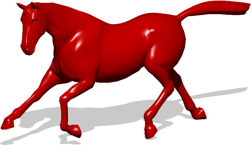
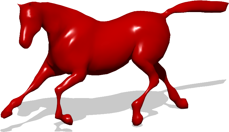
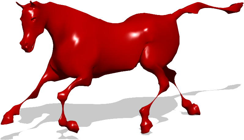
Figure 1: Top: A given horse model. Bottom: The horse coordinates projected to the first 300 LBO eigenfunctions using a regular metric (left), an intermediate metric (middle), and a scale invariant one (right).

We proved that once a proper metric is defined, the Laplace-Beltrami eigenspace is the best possible space for functional approximation of smooth functions. Next, we exploit this property to reformulate classical shape analysis algorithms such as MDS in the spectral domain.

5 Spectral classical scaling

Multidimensional Scaling [7] is a family of data analysis methods that is widely used in machine learning and shape analysis. Given an $\displaystyle n\times n$ pairwise distances matrix $\displaystyle\mathbf{D}$, the MDS method finds an embedding of points of $\displaystyle\mathbb{R}^{m}$, given by an $\displaystyle n\times m$ matrix $\displaystyle\mathbf{X}$, such that the pairwise euclidean distances between every two points, each defined by a row of $\displaystyle\mathbf{X}$, is as close as possible to their corresponding input pair given by the right entry in $\displaystyle\mathbf{D}$. The classical MDS algorithm minimizes the following functional

$$\mathbf{X}=\operatornamewithlimits{argmin~{}}_{\mathbf{X}\in\mathbb{R}^{n\times m}}\left\|\mathbf{X}\mathbf{X}^{T}+\frac{1}{2}\mathbf{J}\mathbf{D}_{2}\mathbf{J}\right\|_{F}$$

where $\displaystyle\mathbf{D}_{2}$ is a matrix such that $\displaystyle(\mathbf{D}_{2})_{ij}=\mathbf{D}^{2}_{ij}$, $\displaystyle\mathbf{J}$ is a centering matrix defined by $\displaystyle\mathbf{J}=\mathbf{I}-\frac{1}{n}\mathds{1}\mathds{1}^{T}$, where $\displaystyle\mathbf{I}$ is the identity matrix, $\displaystyle\mathds{1}$ is a vector of ones, and $\displaystyle\|\cdot\|_{F}$ is the Frobenius norm. The solution can be obtained by a singular value decomposition of the matrix $\displaystyle\mathbf{J}\mathbf{D}_{2}\mathbf{J}$. This method was found to be useful when comparing between isometric shapes using their inter-geodesic distances [14, 9], and texture mapping in computer graphics [34]. The computation of geodesic distances as well as the SVD of an $\displaystyle n\times n$ matrix can be expensive in terms of memory and computational time. High resolution shapes with more than $\displaystyle 10000$ vertices are difficult do handle with this method.

In order to reduce the complexity of the problem, it was proposed in [3] to compute geodesic distances between a small set of sample points, and then, interpolate the rest of the distances by minimizing a bi-harmonic energy in the spectral domain. We find a spectral representation of the matrix $\displaystyle\mathbf{D}_{2}=\mathbf{\Phi}\bm{\alpha}\mathbf{\Phi}^{T}$, where $\displaystyle\mathbf{\Phi}$ represents the matrix that discretizes the spectral domain. We then embed our problem into the eigenspace of the LBO, defining $\displaystyle\mathbf{X}=\mathbf{\Phi}\bm{\beta}$, where $\displaystyle\bm{\beta}$ is an $\displaystyle m\times k$ matrix, and $\displaystyle k\ll n$ in order to reduce the overall complexity. $\displaystyle\mathbf{X}$ is obtained by minimizing

$$\min_{\bm{\beta}}\left\|\mathbf{\Phi}\bm{\beta}\bm{\beta}^{T}\mathbf{\Phi}^{T}+\frac{1}{2}\mathbf{J}\mathbf{\Phi}\bm{\alpha}\mathbf{\Phi}^{T}\mathbf{J}\right\|_{F}.$$

Experimental results of shape canonization comparing shapes flattened with spectral classical scaling to regular classical scaling results were presented in [3]. The spectral approach outperformed the classical scaling in terms of time and space complexities, that lead to overall better accuracy for the spectral version, see Figure 2.

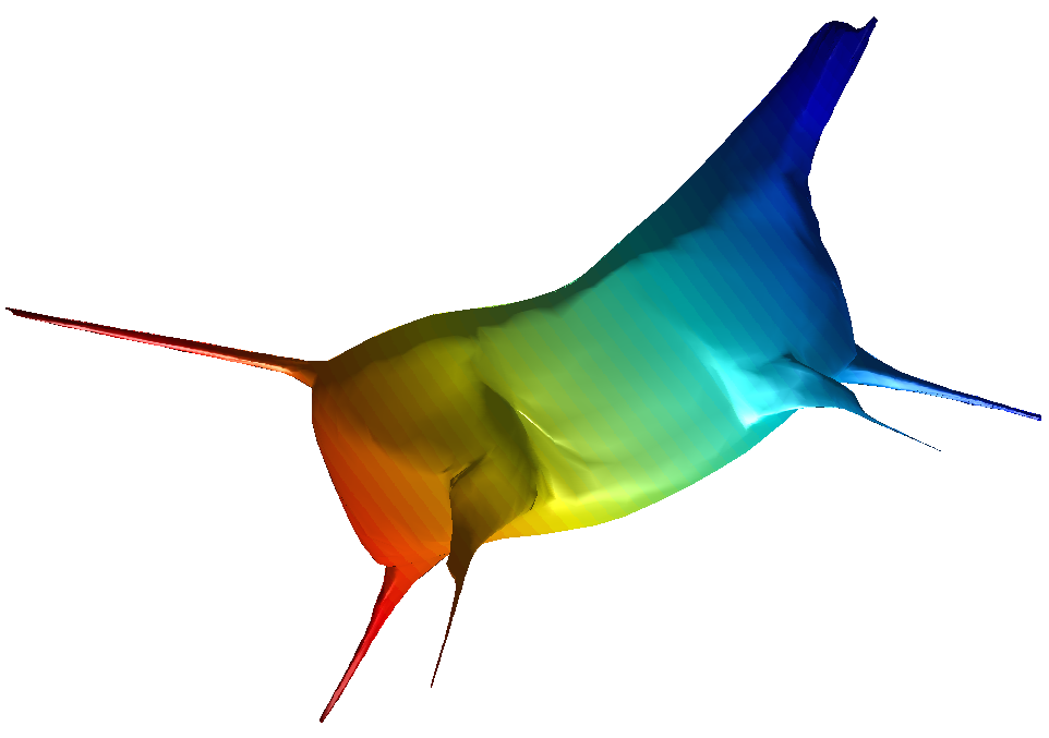
Figure 2: MDS flat embedding: Result of regular MDS (middle) and the spectral MDS (right) of the given horse surface (left).

In the next section we introduce a novel design of functional spaces that benefit from both the Laplace-Beltrami operator and classical principal component analysis, while extending the scope of each of these measures.

6 Regularized PCA

The spectral domain provided by the decomposition of the LBO is efficient in representing smooth functions on the manifold. Still, in some scenarios, functions on manifolds could contain discontinuities that do not align with our model assumption. Alternatively, some functions could be explicitly provided as known points on the data manifold, in which case, the question of what should be the best representation obtains a new flavor. The principal component analysis [17] concept allows to extract a low rank orthonormal approximate representation from a set of such data points $\displaystyle x_{i}$. Given a set of $\displaystyle k$ vectors $\displaystyle x_{i}\in\mathbb{R}^{n}$, the PCA algorithm finds an orthonormal basis of $\displaystyle m\leq k$, defined by its vectors $\displaystyle P_{j}$, by minimizing

$$\begin{array}[]{l}\min_{\mathbf{P}}\sum_{i=1}^{k}\|\mathbf{P}\mathbf{P}^{T}x_{i}-x_{i}\|_{2}^{2}\\ \text{s.t.}\\ \mathbf{P}^{T}\mathbf{P}=\mathbf{I}_{m}.\end{array}$$

It can be shown that this problem can be written as

$$\begin{array}[]{l}\max_{\mathbf{P}}\operatorname{trace}(\mathbf{P}\mathbf{P}^{T}\mathbf{X}\mathbf{X}^{T})\\ \text{s.t.}\\ \mathbf{P}^{T}\mathbf{P}=\mathbf{I}_{m},\end{array}$$

where $\displaystyle\mathbf{X}$ is a matrix whose $\displaystyle i^{th}$ column is the data point $\displaystyle x_{i}$. At the other end, given a manifold $\displaystyle S$, the spectral basis minimizes the Dirichlet energy of any orthonormal basis defined on $\displaystyle S$, where,

$$\begin{array}[]{l}\mathbf{\Phi}=\operatornamewithlimits{argmin~{}}_{\{\psi_{i}\}_{i=1}^{n}}\sum_{i=1}^{n}\|\nabla_{g}\psi_{i}\|_{g}^{2}\cr\text{s.t.}\cr\langle\psi_{i},\psi_{j}\rangle_{g}=\delta_{ij}\,\,\,~{}~{}~{}\forall(i,j),\end{array}$$ (6)

where $\displaystyle\delta_{ij}$ is the Kronecker delta symbol, and $\displaystyle n$ is the number of desired basis functions. Using a discretization of the Laplace-Belrami operator, it can be shown that the PCA and the computation of a spectral basis could be married. We can combine both energies, namely, the energy defined by the data projection error and the Dirichlet energy of the representation space. The result reads,

$$\begin{array}[]{l}\min_{\mathbf{P}}\underbrace{\sum_{i=1}^{m}\|\mathbf{P}\mathbf{P}^{T}\mathbf{A}x_{i}-x_{i}\|_{g}^{2}}_{\text{PCA}}+\mu\underbrace{\sum_{j=1}^{m}\|\nabla_{g}P_{j}\|_{g}^{2}}_{\text{LBO-eigenspace}}\\ \text{s.t.}\\ \mathbf{P}^{T}\mathbf{A}\mathbf{P}=\mathbf{I}_{m}.\end{array}$$ (7)

Where $\displaystyle\mathbf{A}$ represents the local area normalization factor. This problem is equivalent to finding a basis that is both smooth and whose projection error on the set of given vectors (data points) is minimal, as shown in [2] and [16]. When $\displaystyle\mu$ in the above model is set to zero, we have the PCA as a solution. At the other end, as $\displaystyle\mu$ goes to infinity, we get back our LBO eigenbasis domain. The parameter $\displaystyle\mu$ controls the smoothness of the desired basis. The benefits of this hybrid model in representing out of sample information are demonstrated in [2], as can be seen in Figure 3.

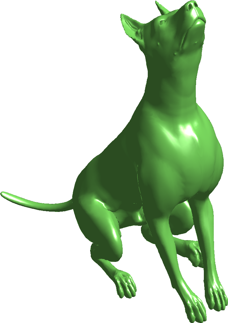
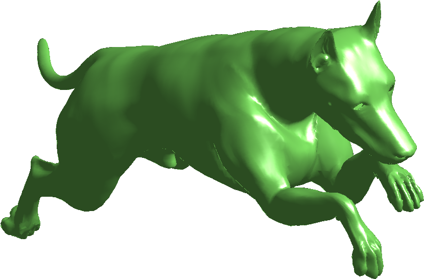
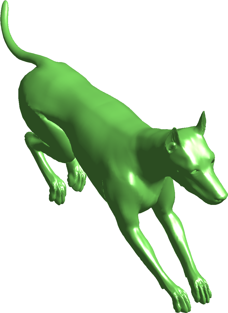
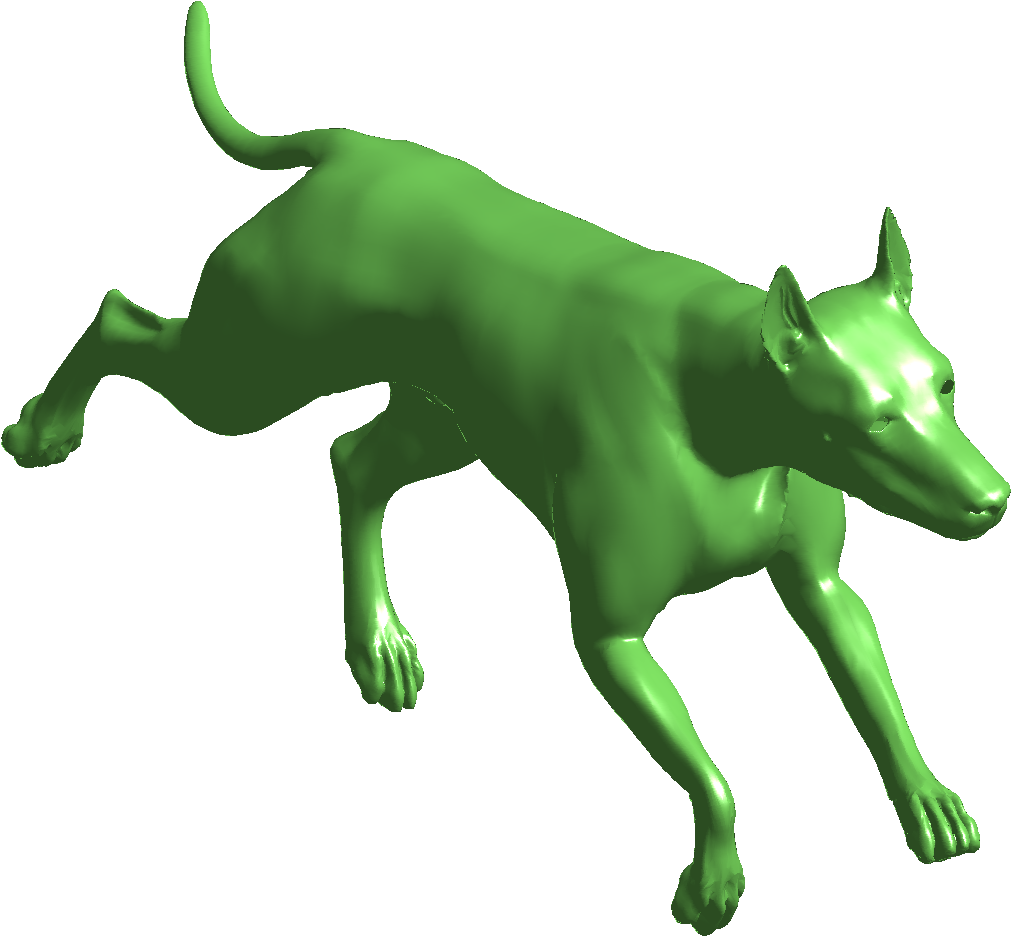
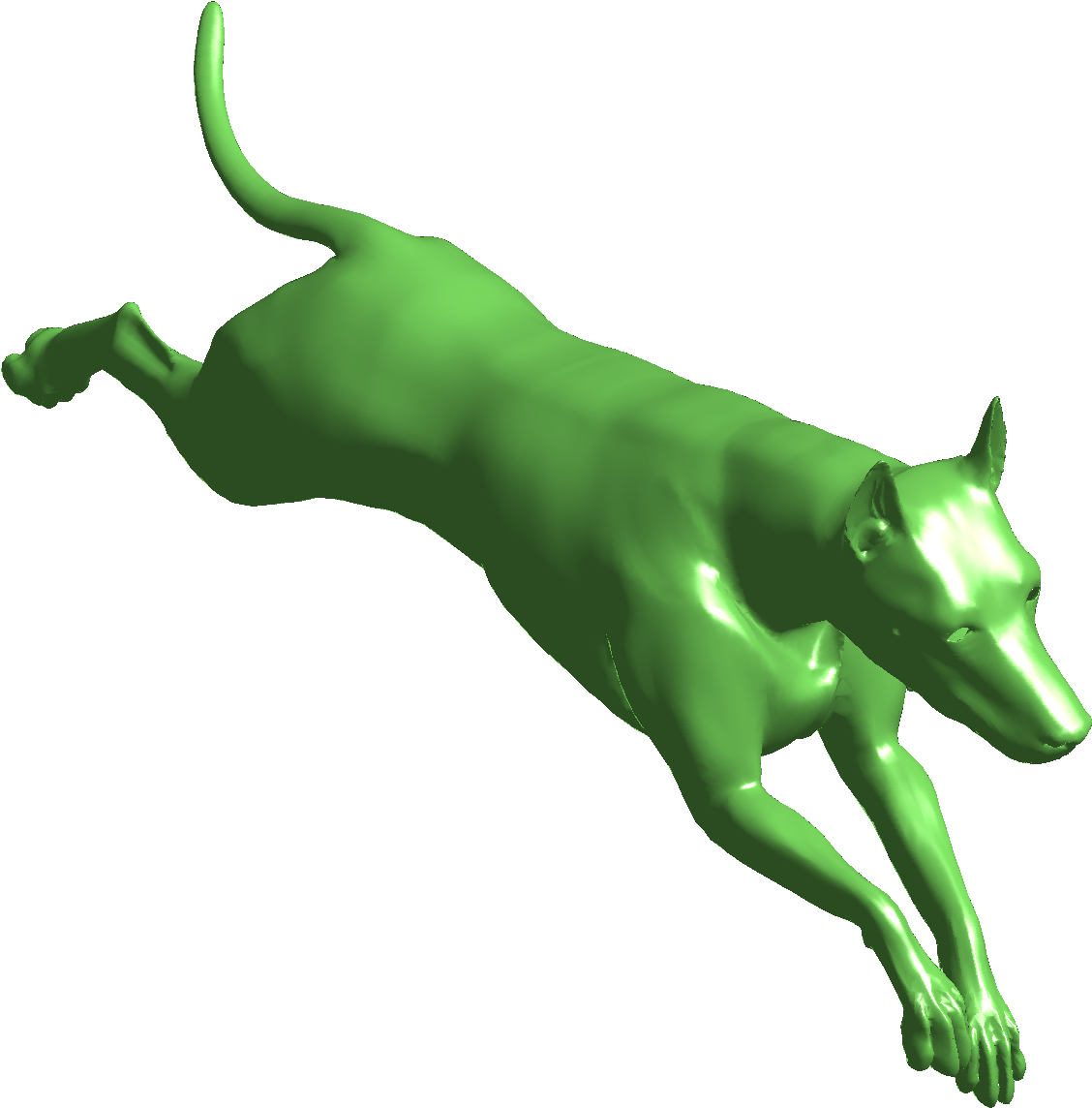
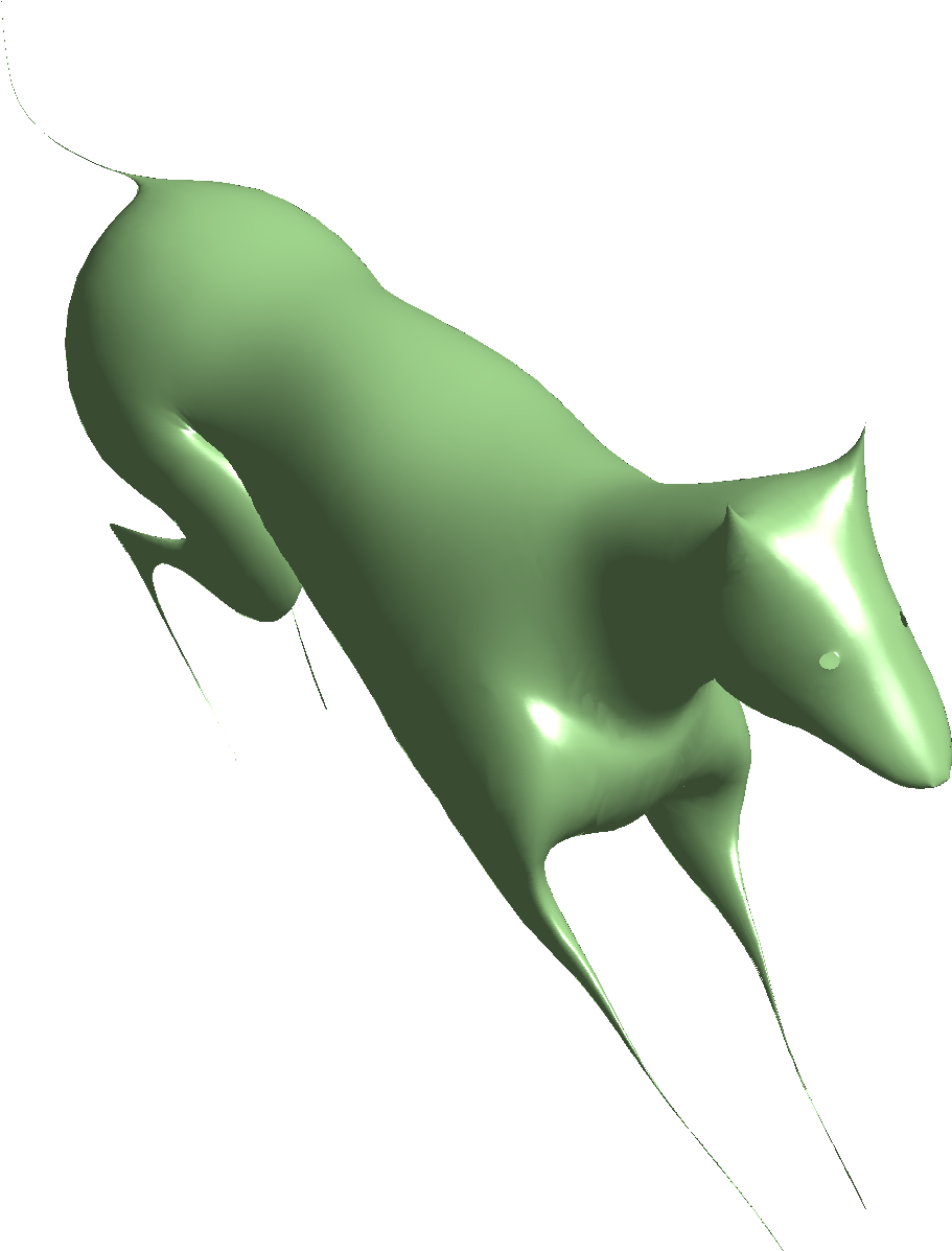
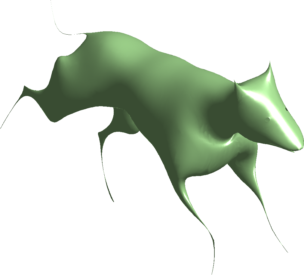
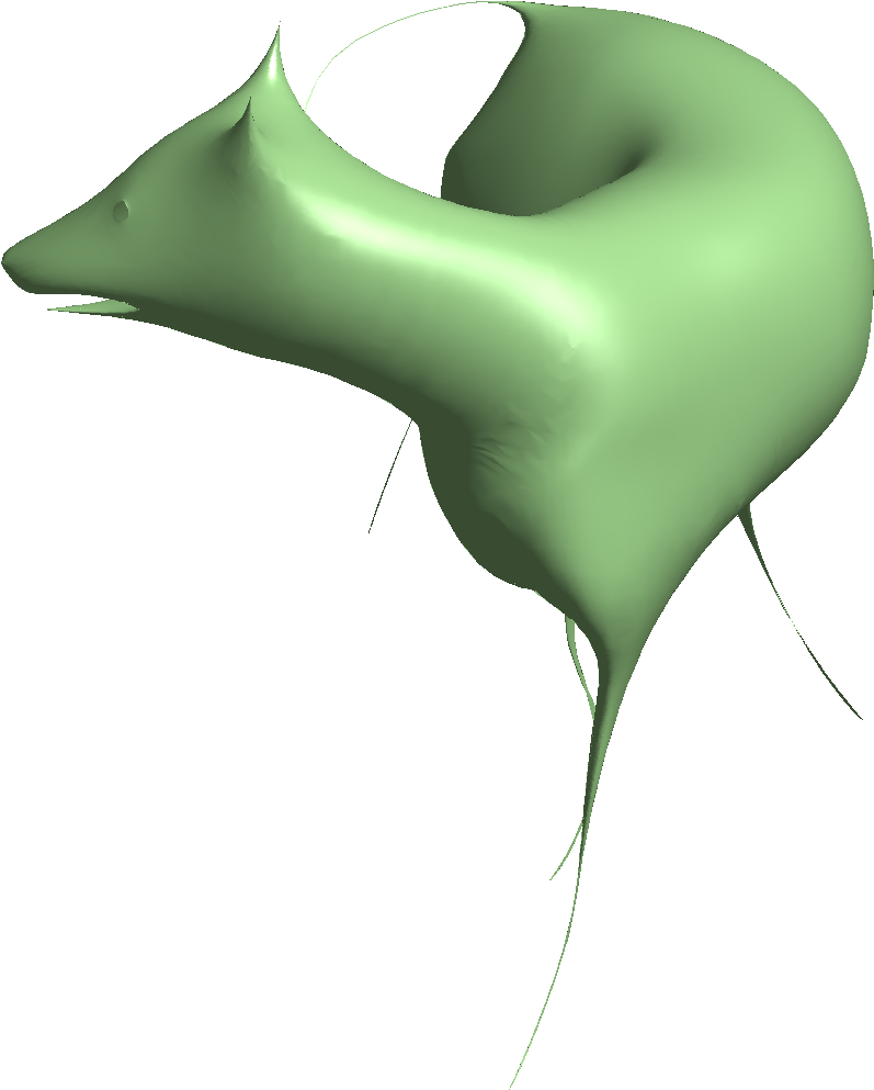
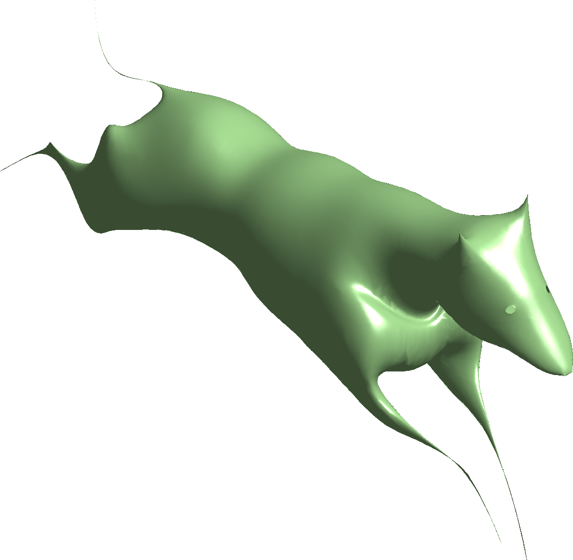
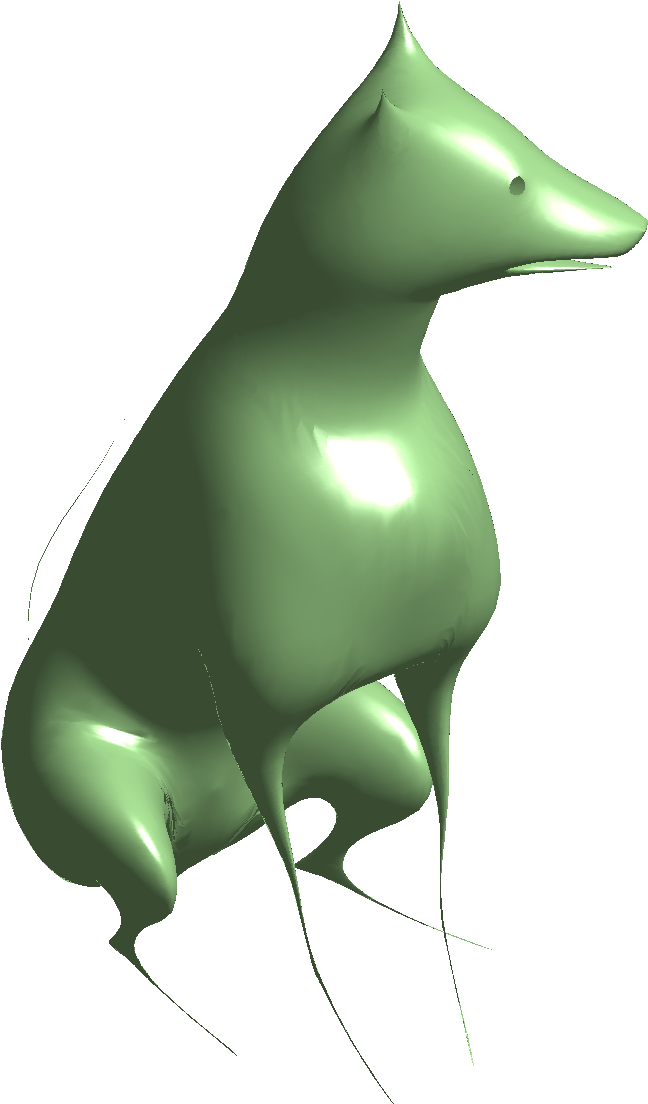
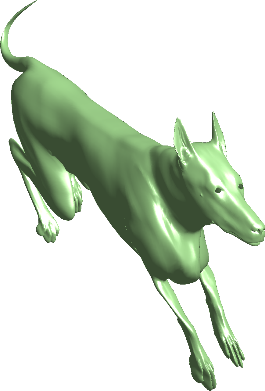
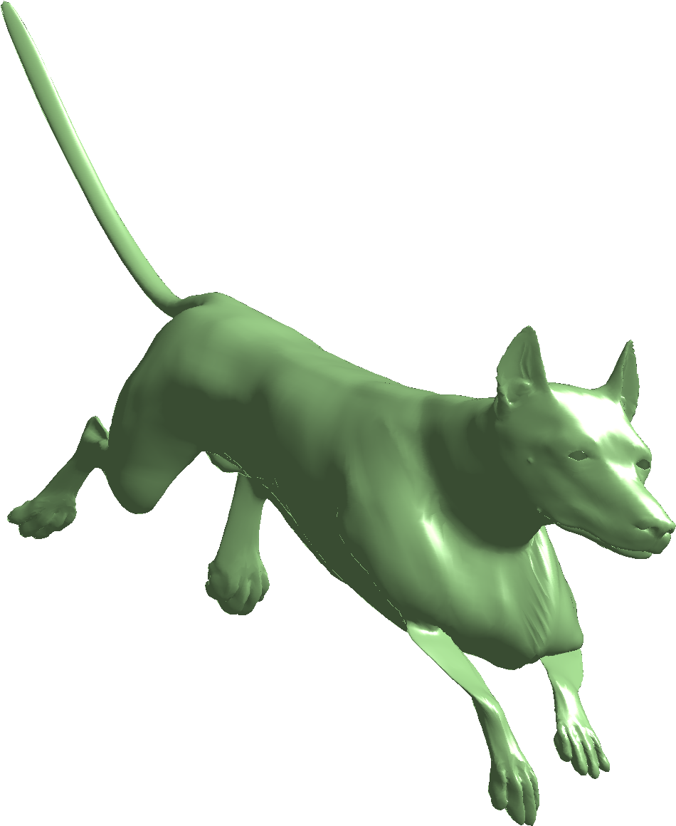
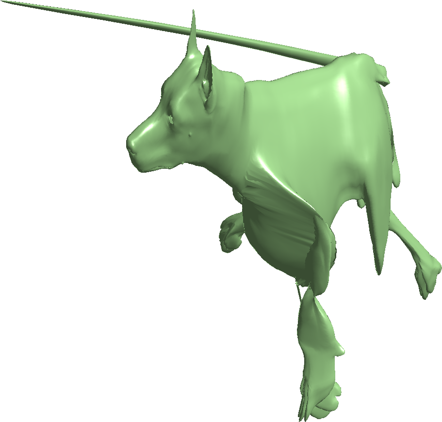
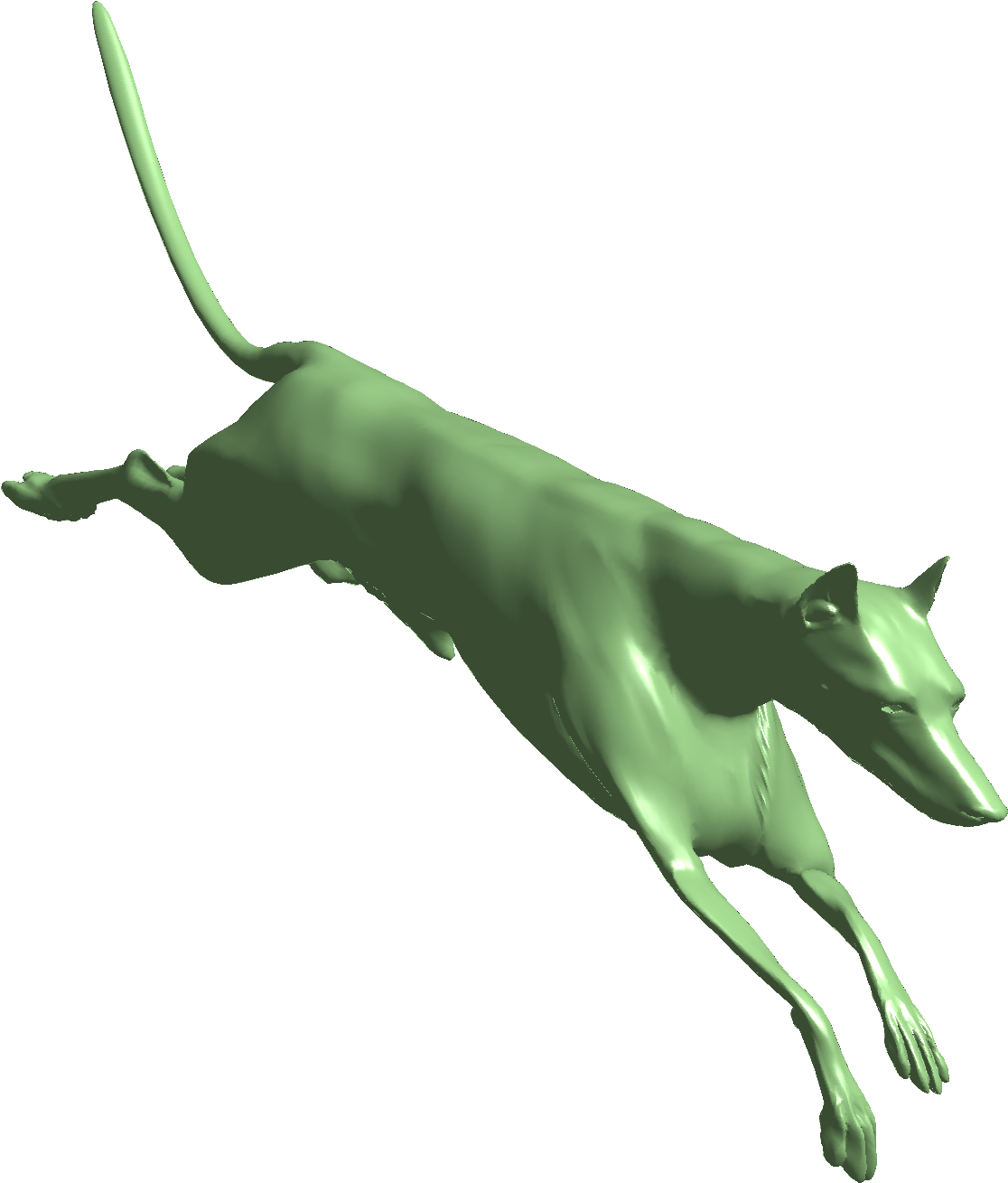
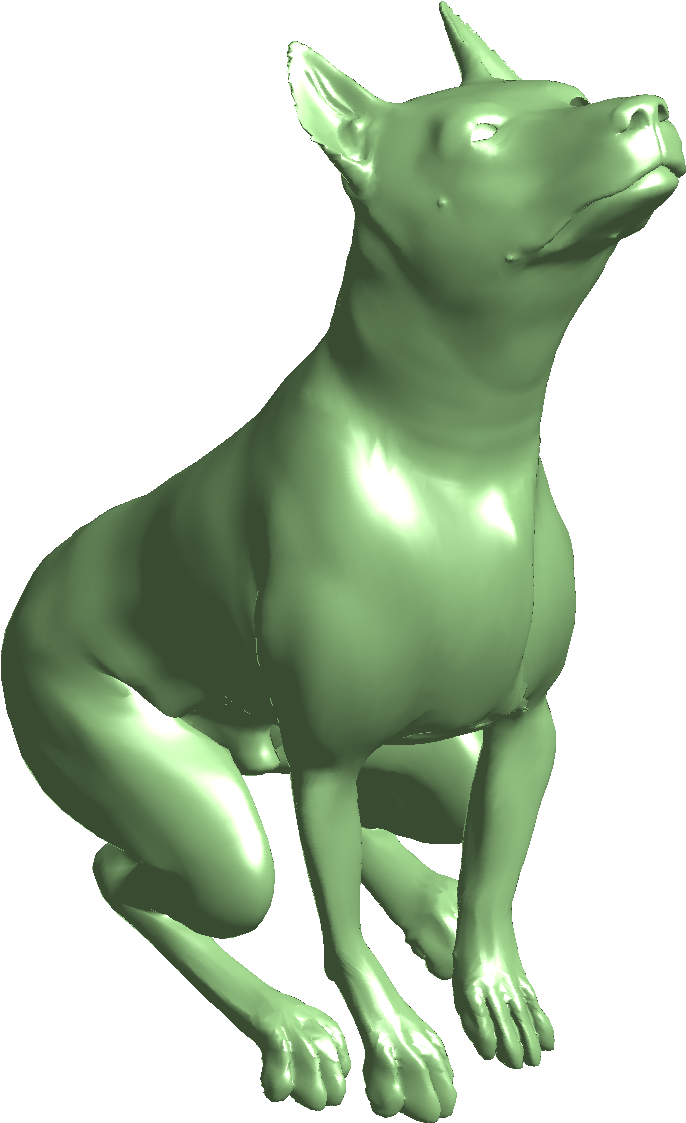
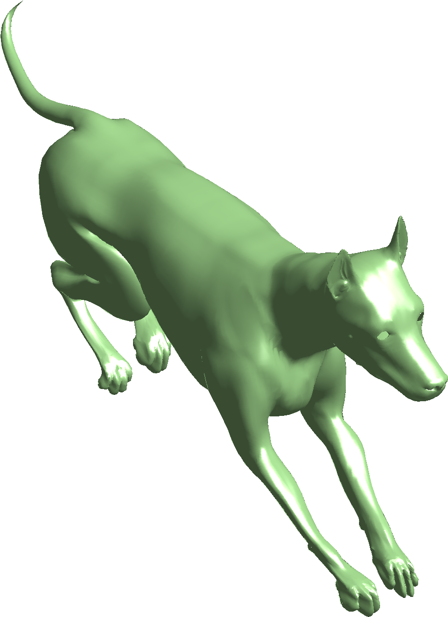
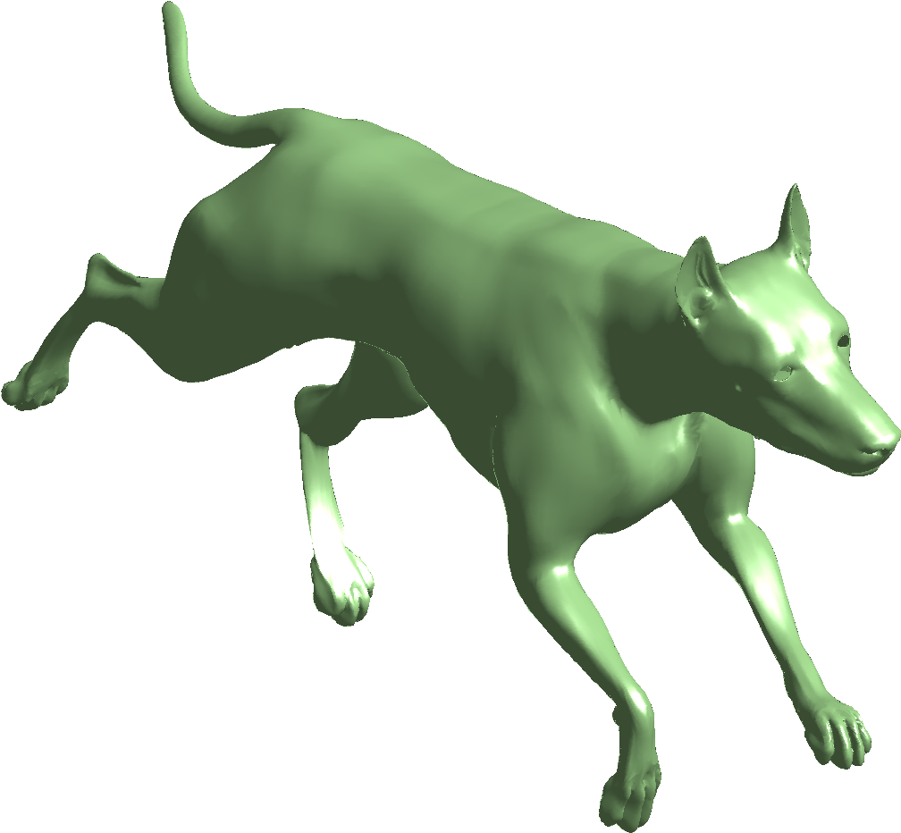
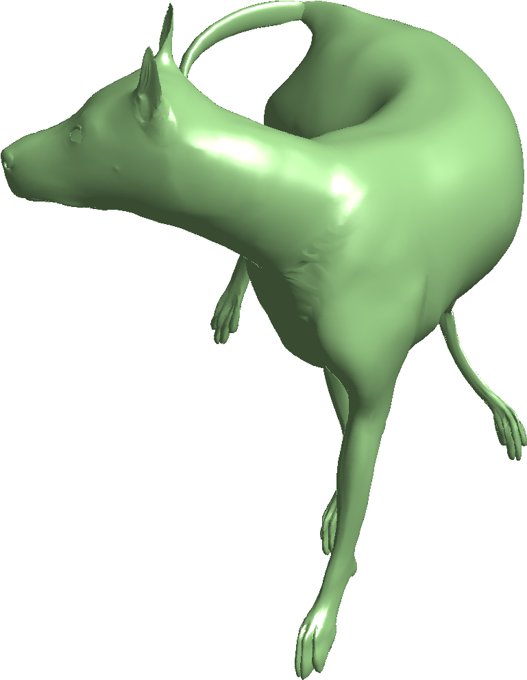
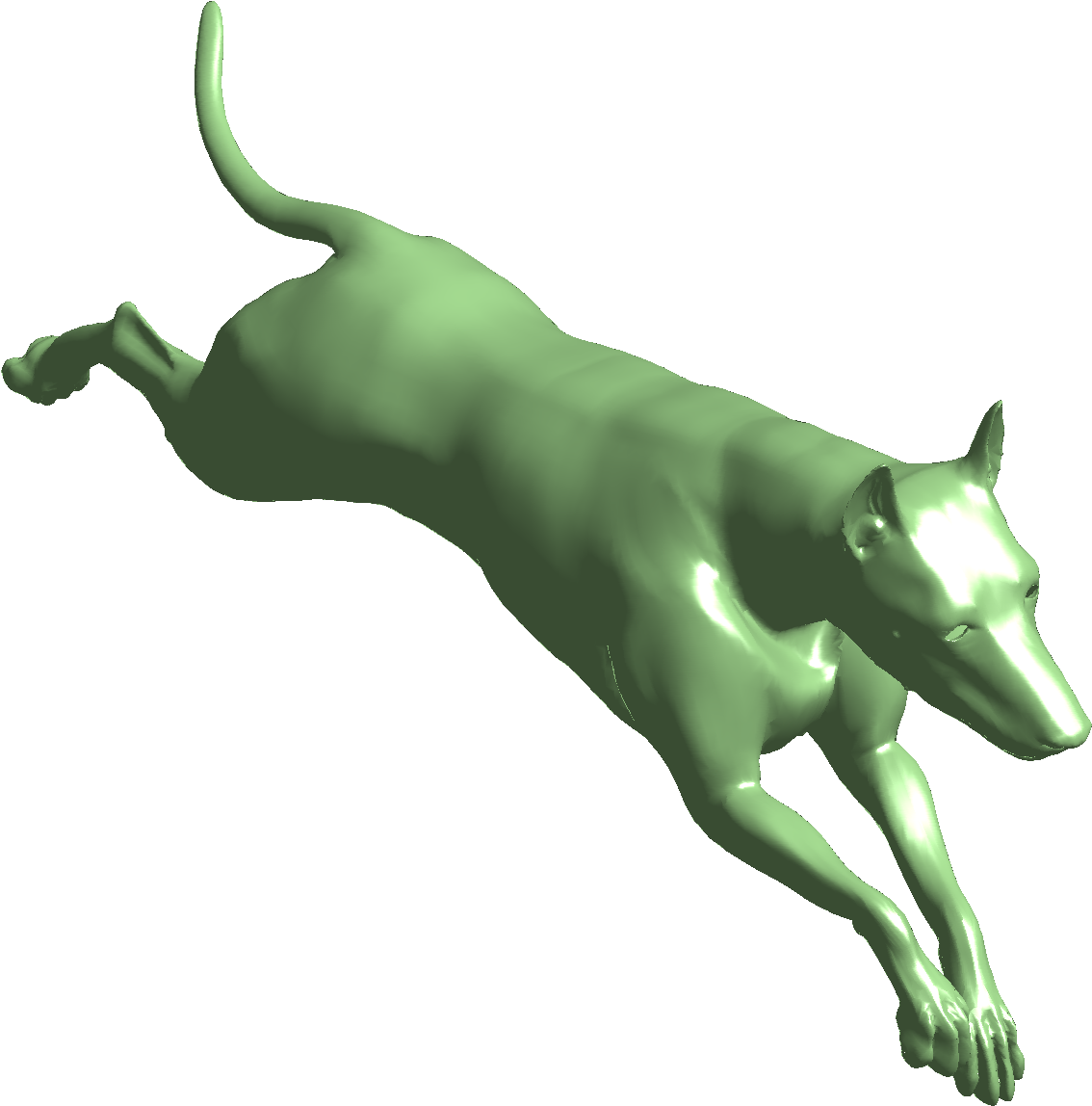
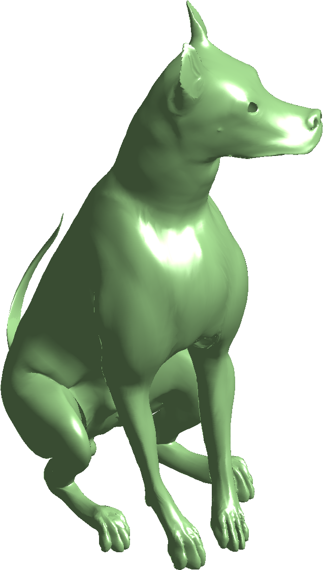
Figure 3: Reconstruction the dog shapes in the second row, by projecting their coordinates to the first $\displaystyle 100$ eigenfunctions of the Laplace-Beltrami (third row), to the PCA basis trained with the two shapes from the first row (forth row), and to the $\displaystyle 100$ basis functions of the regularized-PCA basis trained with the two dogs from the first row (bottom/fifth row).

This model allows us to design an alternative basis which is related to the spectral domain but whose properties can be tuned to fit specific information about the data.

7 Conclusion

A theoretical support for the selection of the leading eigenfunctions of the Laplace-Beltrami operator of a given shape as a natural domain for morphometric study of surfaces was provided. The optimality result motivates the design of efficient shape matching and analysis algorithms. It enabled us to find the most efficient representations of smooth functions on surfaces in terms of both accuracy and complexity when projected onto the first eigenfunctions of the Laplace-Beltrami operator. Our optimality criterion is obviously defined with respect to a given metric. In shape representation, the choice of an appropriate metric is probably as important as the selection of the most efficient sub-space. This was demonstrated in approximating the fine details and the general structure of a shape of a horse in Section 4 using a regular metric, a scale invariant one, and a metric interpolating between the two. Spectral classical scaling and its generalized version, benefit from the presented optimality result, so as the regularization of classical PCA. In both cases it was demonstrated that the decomposition of the LBO provides a natural sub-space to operate in.

The provably optimal representation space allows to construct efficient tools for computational morphometry - the numerical study of shapes. Revisiting the optimality criteria obviously lead to alternative domains and hopefully better analysis tools that we plan to explore in the future.

8 Acknowledgements

YA and RK thank Anastasia Dubrovina, Alon Shtern, Aaron Wetzler, and Michael Zibulevsky for intriguing discussions. This research was supported by the European Community’s FP7- ERC program, grant agreement no. 267414. HB was partially supported by NSF grant DMS-1207793 and also by grant number 238702 of the European Commission (ITN, project FIRST).

Appendix

Theorem .1.

Given a Riemannian manifold $\displaystyle S$ with a metric $\displaystyle(g_{ij})$, the induced LBO, $\displaystyle\Delta_{g}$, and its spectral basis $\displaystyle\phi_{i}$, where $\displaystyle\Delta_{g}\phi_{i}=\lambda_{i}\phi_{i}$, and a real scalar value $\displaystyle 0\leq\alpha<1$, there is no orthonormal basis of functions $\displaystyle\{\psi_{i}\}_{i=1}^{\infty}$, and an integer $\displaystyle n$ such that

$$\left\|f-\sum_{i=1}^{n}\langle f,\psi_{i}\rangle\psi_{i}\right\|_{2}^{2}\leq\alpha\frac{\|\nabla_{g}f\|_{2}^{2}}{\lambda_{n+1}},\,\,\,\,\,\,\,\,\,\,\forall f.$$

To prove the optimality of the LBO eigenbasis, let us first prove the following lemma.

Lemma .1.

Given an orthonormal basis $\displaystyle B=\{b_{1},b_{2},\ldots\}$, of a Hilbert space $\displaystyle\mathcal{V}$, an orthogonal projection operator $\displaystyle P$ of $\displaystyle\mathcal{V}$, such that

$$\|Pv\|\leq k\|v\|,~{}~{}~{}\forall v\in\operatorname{span}{\{b_{i},~{}~{}1\leq i\leq n\}}$$

where $\displaystyle 0<k<1$, then

$$\dim(\ker(P))\geq n.$$

Proof.

Let us denote

$$\begin{array}[]{ll}\mathcal{B}_{1}&=\{b_{i},\|Pb_{i}\|<1\}\\ \mathcal{B}_{2}&=\{b_{i},\|Pb_{i}\|=1\}\\ \mathcal{P}_{1}&=\ker(P)\\ \mathcal{P}_{2}&=\operatorname{im}(P).\end{array}$$

Because the operator $\displaystyle P$ is orthogonal and the basis $\displaystyle B$ is orthonormal, we have

$$\mathcal{V}=\mathcal{B}_{1}\bigoplus\mathcal{B}_{2}=\mathcal{P}_{1}\bigoplus\mathcal{P}_{2},$$

and

$$\begin{array}[]{ll}\mathcal{B}_{1}^{\perp}&=\mathcal{B}_{2}\\ \mathcal{P}_{1}^{\perp}&=\mathcal{P}_{2}.\end{array}$$

By definition, we have that

$$\mathcal{B}_{2}\subset\mathcal{P}_{2}.$$

Then,

$$\mathcal{B}_{2}^{\perp}\supset\mathcal{P}_{2}^{\perp},$$

and since $\displaystyle\mathcal{B}_{2}^{\perp}=\mathcal{B}_{1}$ and $\displaystyle\mathcal{P}_{2}^{\perp}=\mathcal{P}_{1}$, we have

$$\mathcal{P}_{1}\subset\mathcal{B}_{1}.$$

Now, assume that

$$\dim(\mathcal{P}_{1})=\dim(\ker(P))<n\leq\dim\mathcal{B}_{1}$$

Then, $\displaystyle\mathcal{P}_{1}\neq\mathcal{B}_{1}$, and we can find a vector $\displaystyle u\in\mathcal{P}_{1}^{\perp}$ such that $\displaystyle\|u\|=1$ and $\displaystyle u\in\mathcal{B}_{1}$. Since $\displaystyle\mathcal{P}_{1}^{\perp}=\ker(P)^{\perp}=\mathcal{P}_{2}$, it follows that

$$\|Pu\|=1.$$

But, this contradicts the fact that $\displaystyle u\in\mathcal{B}_{1}$, because $\displaystyle u\in\mathcal{B}_{1}$ implies

$$\|Pu\|<1.$$

Then,

$$\dim(\ker(P))\geq n.$$

∎

Equipped with this result we are now ready to prove Theorem A.1

Proof.

Assume that there exists such a basis, $\displaystyle\{\psi_{i}\}$. Then, the representation of a function $\displaystyle f$ in the eigenbasis of the LBO can be written as

$$f=\sum_{i=1}^{\infty}\langle f,\phi_{i}\rangle\phi_{i}=\sum_{i=1}^{\infty}\beta_{i}\phi_{i}.$$

We straightforwardly have

$$\|\nabla_{g}f\|_{2}^{2}=\sum_{i=1}^{\infty}\lambda_{i}\beta_{i}^{2},$$

and it follows that

$$\alpha\frac{\|\nabla_{g}f\|_{2}^{2}}{\lambda_{n+1}}=\sum_{i=1}^{\infty}\underbrace{\frac{\alpha\lambda_{i}}{\lambda_{n+1}}}_{\tilde{\lambda}_{i}}\beta_{i}^{2}=\sum_{i=1}^{\infty}\tilde{\lambda}_{i}\beta_{i}^{2}.$$

Moreover,

$$\left\|f-\sum_{i=1}^{n}\langle f,\psi_{i}\rangle\psi_{i}\right\|_{2}^{2}\leq\alpha\frac{\|\nabla_{g}f\|_{2}^{2}}{\lambda_{n+1}}\leq\sum_{i=1}^{\infty}\tilde{\lambda}_{i}\beta_{i}^{2}.$$

Then, replacing $\displaystyle f$ with $\displaystyle\sum_{j=1}^{n+1}\beta_{j}\phi_{j}$, we have

$$\left\|\sum_{j=1}^{n+1}\beta_{j}\phi_{j}-\sum_{i=1}^{n}\left\langle\sum_{j=1}^{n+1}\beta_{j}\phi_{j},\psi_{i}\right\rangle\psi_{i}\right\|_{2}^{2}\leq\sum_{j=1}^{n+1}\beta_{j}^{2}\tilde{\lambda}_{j}\leq\left(\max_{j=1}^{n+1}\tilde{\lambda}_{j}\right)\left(\sum_{j=1}^{n+1}\beta_{j}^{2}\right),$$

and since $\displaystyle\tilde{\lambda}_{i}<1,~{}~{}\forall i,~{}~{}1\leq i\leq n+1$, we can state that there is a set of $\displaystyle n+1$ orthonormal vectors $\displaystyle\phi_{i}$ belonging to an orthonormal basis whose projection error (over the space spanned by $\displaystyle\psi_{i}$) is smaller than one. According to the previous lemma, the original assumption leads to a contradiction because the dimension of the kernel of the projection on the space spanned by $\displaystyle\psi_{i}$, $\displaystyle\,1\leq i\leq n$, is $\displaystyle n$. ∎

References

- [1] Y. Aflalo, A. Dubrovina, and R. Kimmel. Spectral generalized multi-dimensional scaling. CoRR, abs/1311.2187, 2013.
- [2] Y. Aflalo and R. Kimmel. Regularized PCA. Submitted, 2013.
- [3] Y. Aflalo and R. Kimmel. Spectral multidimensional scaling. Proceedings of the National Academy of Sciences, 110(45):18052–18057, 2013.
- [4] Y. Aflalo, R. Kimmel, and D. Raviv. Scale invariant geometry for nonrigid shapes. SIAM Journal on Imaging Sciences, 6(3):1579–1597, 2013.
- [5] M. Aubry, U. Schlickewei, and D. Cremers. The wave kernel signature: A quantum mechanical approach to shape analysis. In Computer Vision Workshops (ICCV Workshops), 2011 IEEE International Conference on, pages 1626–1633. IEEE, 2011.
- [6] P. Bérard, G. Besson, and S. Gallot. Embedding riemannian manifolds by their heat kernel. Geometric and Functional Analysis, 4(4):373–398, 1994.
- [7] I. Borg and P. Groenen. Modern Multidimensional Scaling: Theory and Applications. Springer, 1997.
- [8] H. Brezis. Functional Analysis, Sobolev Spaces and Partial Differential Equations. Universitext Series. Springer, 2010.
- [9] A. M. Bronstein, M. M. Bronstein, and R. Kimmel. Efficient computation of isometry-invariant distances between surfaces. SIAM Journal on Scientific Computing, 28(5):1812–1836, 2006.
- [10] A. M. Bronstein, M. M. Bronstein, and R. Kimmel. Generalized multidimensional scaling: A framework for isometry-invariant partial surface matching. Proceedings of the National Academy of Sciences, 103(5):1168–1172, 2006.
- [11] A. M. Bronstein, M. M. Bronstein, R. Kimmel, M. Mahmoudi, and G. Sapiro. A gromov-hausdorff framework with diffusion geometry for topologically-robust non-rigid shape matching. International Journal of Computer Vision, 89(2-3):266–286, 2010.
- [12] R. R. Coifman and S. Lafon. Diffusion maps. Applied and Computational Harmonic Analysis, 21(1):5 – 30, 2006. Special Issue: Diffusion Maps and Wavelets.
- [13] R. R. Coifman, S. Lafon, A. B. Lee, M. Maggioni, B. Nadler, F. Warner, and S. W. Zucker. Geometric diffusions as a tool for harmonic analysis and structure definition of data: Diffusion maps. Proceedings of the National Academy of Sciences, 102(21):7426?7431, 2005.
- [14] A. Elad and R. Kimmel. On bending invariant signatures for surfaces. IEEE Trans. Pattern Analysis and Machine Intelligence (PAMI), 25(10):1285–1295, 2003.
- [15] K. Gȩbal, J. A. Bærentzen, H. Aanæs, and R. Larsen. Shape analysis using the auto diffusion function. In Computer Graphics Forum, volume 28, pages 1405–1413. Wiley Online Library, 2009.
- [16] B. Jiang, C. Ding, B. Luo, and J. Tang. Graph-Laplacian PCA: Closed-form solution and robustness. In Computer Vision and Pattern Recognition (CVPR), 2013 IEEE Conference, pages 3492–3498, June 2013.
- [17] I. T. Jolliffe. Principal Component Analysis. Springer, second edition, Oct. 2002.
- [18] Z. Karni and C. Gotsman. Spectral compression of mesh geometry. ACM Transactions on Graphics, pages 279–286, 2000.
- [19] R. Kimmel and J. A. Sethian. Fast marching methods on triangulated domains. Proceedings of the National Academy of Sciences, 95:8341–8435, 1998.
- [20] A. Kovnatsky, M. M. Bronstein, A. M. Bronstein, K. Glashoff, and R. Kimmel. Coupled quasi-harmonic bases. Computer Graphics Forum, 32:439–448, 2013.
- [21] B. Lévy. Laplace-Beltrami eigenfunctions towards an algorithm that “understands” geometry. In Shape Modeling and Applications, 2006. SMI 2006. IEEE International Conference on, pages 13–13. IEEE, 2006.
- [22] F. Memoli and G. Sapiro. A theoretical and computational framework for isometry invariant recognition of point cloud data. Foundations of Computational Mathematics, 5(3):313–347, 2005.
- [23] J. S. B. Mitchell, D. M. Mount, and C. H. Papadimitriou. The discrete geodesic problem. SIAM J. Comput., 16(4):647–668, Aug. 1987.
- [24] M. Ovsjanikov, M. Ben-Chen, J. Solomon, A. Butscher, and L. Guibas. Functional maps: a flexible representation of maps between shapes. ACM Transactions on Graphics, 31(4):1:11, July 2012.
- [25] J. Pokrass, A. M. Bronstein, M. M. Bronstein, P. Sprechmann, and G. Sapiro. Sparse modeling of intrinsic correspondences. Computer Graphics Forum (EUROGRAPHICS), 32:459–268, 2013.
- [26] H. Qiu and E. R. Hancock. Clustering and embedding using commute times. IEEE Trans. Pattern Anal. Mach. Intell., 29(11):1873–1890, Nov. 2007.
- [27] R. Rustamov, M. Ovsjanikov, O. Azencot, M. Ben-Chen, F. Chazal, and L. Guibas. Map-based exploration of intrinsic shape differences and variability. In SIGGRAPH. ACM, 2013.
- [28] J. A. Sethian. A fast marching level set method for monotonically advancing fronts. Proceedings of the National Academy of Sciences, 93:1591–1595, 1996.
- [29] J. Sun, M. Ovsjanikov, and L. Guibas. A concise and provably informative multi-scale signature based on heat diffusion. In Proceedings of the Symposium on Geometry Processing, SGP ’09, pages 1383–1392, Aire-la-Ville, Switzerland, 2009. Eurographics Association.
- [30] V. Surazhsky, T. Surazhsky, D. Kirsanov, S. J. Gortler, and H. Hoppe. Fast exact and approximate geodesics on meshes. ACM Transactions on Graphics, 24(3):553–560, July 2005.
- [31] J. Tsitsiklis. Efficient algorithms for globally optimal trajectories. Automatic Control, IEEE Transactions on, 40(9):1528–1538, Sep 1995.
- [32] H. Weinberger. Variational Methods for Eigenvalue Approximation. Society for Industrial and Applied Mathematics, 1974.
- [33] A. Zaharescu, E. Boyer, K. Varanasi, and R. Horaud. Surface feature detection and description with applications to mesh matching. In Computer Vision and Pattern Recognition, 2009. CVPR 2009. IEEE Conference on, pages 373–380. IEEE, 2009.
- [34] G. Zigelman, R. Kimmel, and N. Kiryati. Texture mapping using surface flattening via multidimensional scaling. Visualization and Computer Graphics, IEEE Transactions on, 8(2):198–207, Apr 2002.