Anomalous radiative transitions

Abstract

Anomalous transitions involving photons derived by many-body interaction of the form, $\partial_{\mu}G^{\mu}$, in the standard model are studied. This does not affect the equation of motion in the bulk, but makes wave functions modified, and causes the unusual transition characterized by the time-independent probability. In the transition probability at a time-interval $T$ expressed generally in the form $P=T\Gamma_{0}+P^{(d)}$, now with $P^{(d)}\neq 0$. The diffractive term $P^{(d)}$ has the origin in the overlap of waves of the initial and final states, and reveals the characteristics of waves. In particular, the processes of the neutrino-photon interaction ordinarily forbidden by Landau-Yang’s theorem ($\Gamma_{0}=0$) manifests itself through the boundary interaction. The new term leads to physical processes over a wide energy range to have finite probabilities. New methods of detecting neutrinos using laser are proposed that are based on this difractive term, which enhance the detectability of neutrinos by many orders of magnitude.

1 Matter wave and $S[\text{T}]$

In modern science and technology, quantum mechanics plays fundamental roles. Despite the fact that stationary phenomena and method have been well developed, those of non-stationary phenomena have not. In the former, the de Broglie wave length ${\hbar\over p}$ determines a typical length and is of a smicroscopic size, and scatterings or reactions in macroscopic scale are considered independent, and successive reactions have been treated under the independent scattering hypothesis. The probability of the event that they occur are computed by the incoherent sum of each value. In the latter, time and space variables vary simultaneously, and a new scale, which can be much larger than the de Broglie wave length, emerges. They appear in overlapping regions of the initial and final waves, and show unique properties of intriguing quantum mechanical waves.

A transition rate computed with a method for stationary waves with initial and final states defined at the infinite time-interval $T=\infty$ is independent of the details of the wave functions. They hold characteristics of particles and preserve symmetry of the system. Transitions occurring at a finite $T$, however, reveal characteristics of waves, the dependence on the boundary conditions [1, 2] , and the probability,

$$P=T\Gamma_{0}+P^{(d)},$$ (1)

where $P^{(d)}$ is the diffractive term which has often escaped attention by researchers. The rate $\Gamma_{0}$ is computed with Fermi’s golden rule [6, 7, 8, 9, 10], and preserves the internal and space-time symmetries, including the kinetic-energy conservation. $\Gamma_{0}$ holds the characteristic properties of particles and the hypothesis of independent scatterings is valid. For a particle of small mass, $m_{s}$, $\Gamma_{0}(p_{i},m_{s})$ behaves

$$\Gamma_{0}(p_{i},m_{s})\approx\Gamma_{0}(p_{i},0),$$ (2)

because the characteristic length, the de Broglie wave length, is determined with $p_{i}$. The region where $P^{(d)}$ is ignorable is called the particle-zone.

Overlapping waves in the initial and final states have the finite interaction energy, and reveal unique properties of waves [1, 2]. Because the interaction energy is part of the total energy, sharing with the kinetic energy, the conservation law of the kinetic-energy is violated. Consequently, the state becomes non-uniform in time and the transition probability has a new component $P^{(d)}$, showing characteristics of waves. The term ${P^{(d)}\over T}$ was shown to behave with a new scale of length, $({\hbar\over m_{s}c})\cdot({E_{i}\over m_{s}c^{2}})$. Accordingly the correction is proportional to the ratio of two small quantities

$${P^{(d)}\over T}=f({1/T\over m_{s}^{2}c^{3}/{\hbar E_{i}}}),$$ (3)

and does not follow Eq. $(\ref{scaling})$.

$P^{(d)}$ reflects the non-stationary waves and is not computed with the stationary waves. In the region where $P^{(d)}$ is important, the hypothesis of independent scattering is invalid, and interference unique to waves manifests. This region is called the wave-zone, and extends to a large area for light particles. $P^{(d)}$ has been ignored, but gives important contributions to the probability in various processes. Especially $P^{(d)}$ is inevitable for the process of $\Gamma_{0}=0$ and $P^{(d)}\neq 0$, which often appears. Furthermore, $P^{(d)}$ can be enhanced drastically, if the overlap of the waves is constructive in wide area. This happens for small $m_{s}$, large $E_{i}$, even for large $T$, and reveals macroscopic quantum phenomena. Processes of large $P^{(d)}$ involving photon and neutrino in the standard model are studied in the present paper.

An example of showing $\Gamma_{0}=0,\ P^{(d)}\neq 0$ is a system of fields described by a free part $L_{0}$ and interaction part $L_{int}$ of total derivative,

$$L=L_{0}+L_{int},\ L_{int}={d\over dt}G,$$ (4)

where $G$ is a polynomial of fields $\phi_{l}(x)$. $\phi_{l}(x)$ follows free equation,

$${\partial L_{0}\over\partial\phi_{l}(x)}-{\partial\over\partial t}{\partial L_{0}\over\partial{\partial\phi_{l}(x)\over\partial t}}=0.$$ (5)

$L_{int}$ decouples from the equation and does not modify the equation of motion in classical and quantum mechanics. Nevertheless, a wave function $|\Psi(t)\rangle$ follows a Schrödinger equation in the interaction picture,

$$i\hbar{\partial\over\partial t}|\Psi\rangle_{int}=({\partial\over\partial t}G_{int}(t))|\Psi\rangle_{int},$$ (6)

where the free part, $H_{0}$, and the interaction part, $H_{int}$, are derived from the previous Lagrangian, and $G_{int}$ stands for $G$ of the interaction picture. A solution at $t$,

$$|\Psi(t)\rangle_{int}=e^{G_{int}(t)-G_{int}(0)\over i\hbar}|\Psi(0)\rangle_{int},$$ (7)

is expressed with $G(t)$, and the state at $t>0$ is modified by the interaction. The initial state $|\Psi(0)\rangle_{int}$ prepared at $t=0$ is transformed to the other state of t-independent weight. Hence, Eq. $(\ref{quasi-statioinary})$, is like stationary, and $\Gamma_{0}=0$ , and $P^{(d)}\neq 0$. Physical observables are expressed by the probability of the events, which are specified by the initial and final states. For those at finite $T$, normal S-matrix, $S[\infty]$, which satisfies the boundary condition at $T=\infty$ instead of those at finite $T$, is useless. $S[T]$ that satisfies the boundary condition at $T$ [1, 2] is necessary and was constructed. $S[T]$ is applied to the system described by Eq. $({\ref{total-derivative}})$.

$S[T]$ is constructed with the Møller operators at a finite $T$, $\Omega_{\pm}({T})$, as $S[T]=\Omega_{-}^{\dagger}(T)\Omega_{+}(T)$. $\Omega_{\pm}({T})$ are expressed by a free Hamiltonian $H_{0}$ and a total Hamiltonian $H$ by $\Omega_{\pm}(T)=\displaystyle\lim_{t\rightarrow\mp T/2}e^{iHt}e^{-iH_{0}t}$. From this expression, $S[T]$ is unitary and satisfies

$$[S[T],H_{0}]\neq 0,$$ (8)

hence a matrix element of $S[T]$ between two eigenstates of $H_{0}$, $|\alpha\rangle$ and $|\beta\rangle$ of eigenvalues $E_{\alpha}$ and $E_{\beta}$, is decomposed into two components

$$\langle\beta|S[{T}]|\alpha\rangle=\langle\beta|S^{(n)}[{T}]|\alpha\rangle+\langle\beta|S^{(d)}[{T}]|\alpha\rangle,$$ (9)

where $\langle\beta|S^{(n)}|\alpha\rangle$ and $\langle\beta|S^{(d)}|\alpha\rangle$ get contributions from cases $E_{\beta}=E_{\alpha}$ and $E_{\beta}\neq E_{\alpha}$, and give $\Gamma_{0}\text{T}$ and $P^{(d)}$ respectively. The deviation of the kinetic-energies, $E_{\beta}-E_{\alpha}$, in the latter is due to the interaction energy of the overlapping waves, which depends on the coordinate system. Therefore, it is understood that $H_{int}$ is not Lorentz invariant. Thus the kinetic-energy non-conserving term, which was mentioned by Pierls and Landau [4] so as to give negligibly small correction, yields $P^{(d)}$ [5] . Because $H_{0}$ is an generator of the Poincare group, Eq.$(\ref{commutation-relation})$ shows that $S^{(d)}[\text{T}]$ and $P^{(d)}$ violate the Poincare invariance. In the system described by Eq. $({\ref{total-derivative}})$, the first term disappears but the second term does not, $\Gamma_{0}=0$, and $P^{(d)}\neq 0$.

$S[T]$ is expressed with the boundary conditions for the scalar field $\phi(x)$ [12, 13],

$$\lim_{t\rightarrow-T/2}\langle\alpha|\phi^{f}|\beta\rangle=\langle\alpha|\phi_{in}^{f}|\beta\rangle,$$ (10)

$$\lim_{t\rightarrow+T/2}\langle\phi^{f}|0\rangle=\langle\alpha|\phi_{out}^{f}|\beta\rangle,$$ (11)

where $\phi_{in}(x)$ and $\phi_{out}(x)$ satisfy the free wave equation, and $\phi^{f},\ \phi_{in}^{f},\ \text{and}\ \phi_{out}^{f}$ are the expansion coefficient of $\phi(x),\ \phi_{in}(x),\ \text{and}\ \phi_{out}(x)$, with the normalized wave functions $f(x)$ of the form

$$\phi^{f}(t)=i\int d^{3}xf^{*}({\vec{x}},t)\overleftrightarrow{\partial_{0}}\phi({\vec{x}},t).$$ (12)

The function $f(x)$ indicates the wave function that the out-going wave interacts in a successive reaction of the process. The out-going photon studied in the following section interacts with atom or nucleus and their wave functions are used for $f(x)$. Consequently, $S^{(d)}[T]$ depends on $f(x)$, and is appropriate to write as $S^{(d)}[T;f]$. Accordingly the probability of the events is expressed by this normalized wave function, called wavepacket. Wavepackets that satisfy free wave equations and are localized in space are important for rigorously defining scattering amplitude [12, 13]. $S^{(d)}[T;f]$ expresses the wave nature due to the states of continuous kinetic-energy. $S^{(d)}[T;f]$ does not preserve Poincaré invariance defined by $L_{0}$. The state $|\beta\rangle$ of $E_{\beta}$ is orthogonal to $|\alpha\rangle$ of $E_{\alpha}\neq E_{\beta}$ and $P^{(d)}$ approaches constant at $T=\infty$.

The wavepackets [12, 13, 8, 9, 10] can be replaced with plane waves for a practical computation for $S[\infty]$ [18, 19, 20, 21, 22, 23, 24, 25], but can not be done so for $P^{(d)}$ [14, 15, 16]. $P^{(d)}$ is derived from $S^{(d)}[T;f]$, and depends on $f(x)$.

Photon is massless in vacuum and has a small effective mass determined by the plasma frequency in matter, and neutrino is nearly massless. Thus they have the large wave-zone of revealing wave phenomena caused by $P^{(d)}$. These small masses make $P^{(d)}$ appear in a macroscopic scale and significantly affect physical reactions. In this small (or zero) mass region the effects of diffractive term $P^{(d)}$ are pronounced. This is our interest in the present paper. The produced photon interacts with matter with the electromagnetic interaction, which leads to macroscopic observables. The term $P^{(d)}$ of the processes of $\Gamma_{0}=0$ such as $2\gamma$ decays of $1^{+}$ meson and $\gamma$ and ${\nu}$ reactions are shown to be relevant to many physical processes, including possible experimental observation of relic neutrino. The enhancement of the probability for light particles with intense photons based on the normal component $\Gamma_{0}$ was proposed in Refs. [27, 28], and the collective interaction between electrons and neutrino derived from the normal component $\Gamma_{0}$ was considered in Ref. [29]. Our theory is based on the probability $P^{(d)}$, hence differs from the previous ones in many respects.

This paper is organized in the following manner. In Section 2, the couplings of two photon with $1^{+}$ state through triangle diagram is obtained. In section 3 and 4, positronium and heavy quarkonium are studied and their $P^{(d)}$ are computed. Based on these studies we go on to investigate the interaction of photons and neutrinos. In section 5, neutrino–photon interaction of the order $\alpha G_{F}$, and various implications to high energy neutrino phenomena are presented. In Section 6 we explore the implication of the photon-neutrino coupling on experimental settings. Summary is given in section 7.

2 Coupling of $1^{+}$ meson with two photons

The coupling of $\gamma\gamma$ with axial vector states, $1^{+}$ meson composed of $e^{-}e^{+}$, $Q\bar{Q}$, and $\nu\bar{\nu}$ are studied using an effective Lagrangian expressed by local fields. From symmetry considerations, an effective interaction of the $1^{+}$ state $\phi_{1}^{\mu}$ with two photons has the form,

$$S_{int}=g\int d^{4}x\partial_{\mu}(\phi_{1}^{\mu}(x)\tilde{F}_{\alpha\beta}(x)F^{\alpha\beta}(x)),$$ (13)

$$\partial_{\mu}\phi_{1}^{\mu}(x)=0,\tilde{F}_{\alpha\beta}(x)=\epsilon_{\alpha\beta\gamma\nu}F^{\gamma\nu}(x),$$

where $F_{\alpha\beta}$ is the electromagnetic field, and the coupling strength $g$ is computed later. In a transition of plane waves in infinite-time interval, the space-time boundary is at the infinity, and the transition amplitude is computed with the plane waves, in the form,

$$M=(p_{i}-p_{f})_{\mu}(2\pi)^{4}\delta(p_{i}-p_{f})\tilde{M}^{\mu}$$ (14)

and vanishes, where $p_{i}$ and $p_{f}$ are four-dimensional momenta of the initial and final states and $\tilde{M}$ is the invariant amplitude. This shows that the amplitude proportional to $\delta^{4}(p_{i}-p_{f})$ and the transition rate $\Gamma_{0}$ vanish. The rate of $1^{+}\rightarrow\gamma\gamma$ decay vanishes in general systems, because the state of two photons of momenta $(\vec{p},-\vec{p})$ does not couple with a massive $1^{+}$ particle. Hence

$$\Gamma_{0}^{1^{+}\rightarrow\gamma\gamma}=0,$$ (15)

which is known as Landau-Yang’s theorem [30, 31].

The term $S_{int}$ is written as a surface term in four-dimensional space-time,

$$S_{int}=\int_{surface}d{S_{\mu}}g(\phi_{1}^{\mu}(x)\tilde{F}_{\alpha\beta}(x)F^{\alpha\beta}(x)),$$ (16)

which is determined by the wave functions of the initial and final states. Accordingly, the transition amplitude derived from this surface action is not proportional to $T$, but has a weaker $T$ dependence. Thus $P^{(d)}$ comes from the surface term, and does not have the delta function of kinetic-energy conservation. Kinetic energy of the final states deviates from that of the initial state due to the finite interaction energy between them. The deviation becomes larger and $P^{(d)}$ is expected to increase with larger overlap. We find $P^{(d)}$ in the following.

2.1 Triangle diagram

The interaction of the form Eq. $(\ref{effective-interaction})$ is generated by one loop effect in the standard model. The scalar and axial vector current

$$J(0)=\bar{l}(0)l(0),$$ (17)

$$J^{5,\mu}=\bar{l}(0)\gamma_{5}\gamma^{\mu}l(0)$$ (18)

in QED, we have

$$L=L_{0}+L_{\text{int}},\ L_{0}=\bar{l}(x)(\gamma\cdot p-m_{l})l(x)-{1\over 4}F_{\mu\nu}(x)F^{\mu\nu}(x),$$ (19)

$$L_{\text{int}}=eJ_{\mu}A^{\mu}(x),\ J_{\mu}(x)=\bar{l}(x)\gamma_{\mu}l(x),$$

where $A^{\mu}(x)$ is the photon field and $l(x)$ is the electron field, coupled through two photons in the bulk through the triangle diagram Fig. 1. The matrix elements are

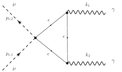
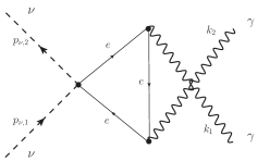
Figure 1: Triangle diagrams of the electron loop which give contributions to $1^{+}(l\bar{l})\rightarrow\gamma\gamma$, $\nu+\gamma\rightarrow\nu+\gamma$ and $\nu+\bar{\nu}\rightarrow\gamma+\gamma$.

$$\Gamma_{0}=\langle 0|J(0)|k_{1},k_{2}\rangle={e^{2}\over 4\pi^{2}}\epsilon^{\mu}(k_{1})\epsilon^{\nu}(k_{2})m[k_{2,\mu}k_{1\nu}-g_{\mu\nu}k_{1}\cdot k_{2}]f_{0},$$ (20)

$$\Gamma_{5,\alpha}=\langle 0|J_{5,\alpha}(0)|k_{1},k_{2}\rangle=-i{e^{2}\over 4\pi^{2}}2f_{1}\epsilon^{\mu_{1}}(k_{1})\epsilon^{\mu_{2}}(k_{2})$$

$$\times[(k_{1,\mu_{2}}\epsilon_{\mu_{1}\nu_{1}\nu_{2}\alpha}-k_{2,\mu_{1}}\epsilon_{\mu_{2}\nu_{1}\nu_{2}\alpha})k_{1}^{\nu_{1}}k_{2}^{\nu_{2}}+(k_{1}\cdot k_{2})\epsilon_{\mu_{1}\mu_{2}\nu\alpha}(k_{1}-k_{2})^{\nu}],$$ (21)

where $\epsilon_{\mu}(k)$ is the polarization vector for the photon. The triangle diagram for the axial vector current Eq. (2.1) has been studied in connection with axial anomaly and $\pi^{0}\rightarrow\gamma\gamma$ decay [32, 33, 34, 35, 36] and now is applied to $P^{(d)}$ for two photon transitions of the axial vector meson and neutrino. The triangle diagram Fig. 1 shows that the interaction occurs localy in space and time, but the transition amplitude is the integral over the coordinates and receives the large diffractive contribution if the neutrino and photon are spatially spread waves. In Fig. 1, the in-coming and out-going waves are expressed by lines, but they are in fact the spread waves, which is obvious in the figures in Ref. [37] and in Fig. 2.

$\Gamma_{5,\alpha}$ is expressed also with $f_{1}$ in the form

$$\Gamma_{5,\alpha}=\frac{\alpha_{em}}{2\pi}f_{1}(k_{1}+k_{2})_{\alpha}(\tilde{F}_{1,\rho\lambda}F_{2}^{\rho\lambda}+\tilde{F}_{2,\rho\lambda}F_{1}^{\rho\lambda}),$$ (22)

$$F_{1,\rho\lambda}=k_{1,\rho}\epsilon_{1,\lambda}-k_{1,\lambda}\epsilon_{2,\rho},\tilde{F}_{\rho\lambda}={1\over 2}\epsilon_{\rho\lambda\xi\eta}F^{\xi\eta}.$$

The coefficients $f_{0}$ and $f_{1}$ are given by the integral over the Feynman parameters,

$$f_{0}=\int_{0}^{1}dx\int_{0}^{1-x}dy{1\over m_{l}^{2}-2xyk_{1}\cdot k_{2}-i\epsilon},$$ (23)

$$f_{1}=\int_{0}^{1}dx\int_{0}^{1-x}dy{xy\over m_{l}^{2}-2xyk_{1}\cdot k_{2}-i\epsilon},$$ (24)

where

$$f_{1} = -{1\over 4k_{1}\cdot k_{2}}+{m_{l}^{2}\over 4(k_{1}\cdot k_{2})^{2}}I_{1},$$ (25)

$$I_{1} = 2k_{1}\cdot k_{2}\int_{0}^{1}dx\int_{0}^{1-x}dy{1\over m_{l}^{2}-2xyk_{1}\cdot k_{2}-i\epsilon}$$ (26)

$$= \begin{cases}2\text{Sin}^{-1}\left(\sqrt{k_{1}\cdot k_{2}\over 2m_{l}^{2}}\right),\ \text{if}~{}k_{1}\cdot k_{2}<2m_{l}^{2},\\ {\pi^{2}\over 2}-{1\over 2}\log^{2}{1+\sqrt{1-{2m_{l}^{2}\over k_{1}\cdot k_{2}}}\over 1-\sqrt{1-{2m_{l}^{2}\over k_{1}\cdot k_{2}}}}+i\pi\log{1+\sqrt{1-{2m_{l}^{2}\over k_{1}\cdot k_{2}}}\over 1-\sqrt{1-{2m_{l}^{2}\over k_{1}\cdot k_{2}}}},\ \text{if}~{}k_{1}\cdot k_{2}\geq 2m_{l}^{2}.\end{cases}$$

$f_{1}$ in various kinematical regions is

$$f_{1}=\begin{cases}{-1\over 4k_{1}\cdot k_{2}}+{m^{2}\over 4(k_{1}\cdot k_{2})^{2}}\pi(1-{2\delta E\over m_{l}});\ k_{1}\cdot k_{2}=2m_{l}^{2}-m_{l}\delta E,\\ {-1\over 4k_{1}\cdot k_{2}};\ k_{1}\cdot k_{2}\gg m_{l}^{2},\\ {1\over 2m_{l}^{2}};\ k_{1}\cdot k_{2}\ll m_{l}^{2}.\end{cases}$$ (27)

Figure 2: Diagram of the neutrino photon scattering, $\nu+\gamma\rightarrow\nu+\gamma$ of spatially spread waves.

3 Positronium

The bound states of a positronium with the orbital angular momentum $L=1,S=1$ have total angular momentum $J=2,1,0$. These states at rest of ${\vec{P}}=0$ are expressed with non-relativistic wave functions and creation operators of $l^{+}$ and $l^{-}$ of momentum ${\vec{p}}$, spin $\pm 1/2$, and P-wave wave functions $p_{i}F(p)$ as are given in Appendix A, where

$$|1/2,1/2;-1\rangle=\int d{\vec{p}}\,b_{+1/2}^{\dagger}({\vec{p}}\,)d_{+1/2}^{\dagger}(-{\vec{p}}\,)(p_{x}-ip_{y})F(p)|0\rangle.$$ (28)

Others are defined in the same manner.

These bound states couple with the lepton pairs with effective local interactions which are expressed as

$$L_{int}=g_{0}\phi_{0}(x)\bar{l}(x)l(x)+g_{1}\phi_{1}^{\mu}(x)\bar{l}(x)\gamma^{5}\gamma_{\mu}l(x)+g_{2}\phi_{2}^{\mu\nu}(x)\bar{l}(x)\gamma_{\mu}\partial_{\nu}l(x),$$ (29)

where the coupling strengths are computed from

$$g_{0}=\langle 0|\bar{l}(0)l(0)|\phi_{0};{\vec{p}}=0\rangle,$$ (30)

$$g_{1}\epsilon^{\mu}({\vec{p}}=0)=\langle 0|\bar{l}(0)\gamma^{5}\gamma^{\mu}l(0)|\phi_{1};{\vec{p}}=0\rangle,$$ (31)

$$g_{2}\epsilon^{\mu\nu}({\vec{p}}=0)=\langle 0|\bar{l}(0)\gamma^{\mu}{\partial}^{\nu}l(0)|\phi_{2};\vec{p}=0\rangle,$$ (32)

where the $\epsilon^{\mu},\epsilon^{\mu\nu}$ are polarization vector or tensor for the massive vector and tensor mesons. We have

$$g_{0}=gN_{0},g_{1}=gN_{1},g_{2}=gN_{2},$$ (33)

$$g=-2\pi\int dp\,p^{4}F(p){2\over|E|+m},$$

$$N_{0}=1,\ N_{1}=0.862,\ N_{2}=1.33.$$

The decay rates for $0^{+}$ and $2^{+}$ were studied in [38, 39], so that here we concentrate on $1^{+}$ and $0^{+}$ as a reference for $1^{+}$.

Fields $\phi_{0}(x),\phi_{1}(x),\text{ and }\phi_{2}(x)$ couple with two photons through the triangle diagrams. Their interactions with two photons are summarized in the following effective Lagrangian,

$$L_{int}=g_{0}{\alpha\over\pi}f_{0}\phi_{0}F_{\mu\nu}F^{\mu\nu}+g_{1}{\alpha\over\pi}f_{1}\partial_{\mu}(\phi_{1}^{\mu}\epsilon_{\nu\rho\sigma\tau}F^{\nu\rho}F^{\sigma\tau})+g_{2}{\alpha\over\pi}T^{\mu\nu}F_{\mu\rho}F^{\rho\nu}.$$

3.1 Axial vector positronium

Here we study the two photon decay of axial vector positronium, which is governed by the second term of the right-hand side of Eq. $(\ref{effective-two-photon})$. The matrix element of the axial current between the vacuum and two photon state was computed by Refs. [32, 33, 34, 35, 36]. Because $\Gamma_{0}$ of two photon decay of axial vector meson vanishes due to Landau-Yang’s theorem, but $P^{(d)}$ does not, we give the detailed derivation of $P^{(d)}$.

From the effective interaction, Eq. $(\ref{effective-two-photon})$, the probability amplitude of the event that one of the photons of ${\vec{k}}_{\gamma}$ from the decay of $c_{\mu}$ of $\vec{p}_{c}$ is detected at $({\vec{X}}_{\gamma},T_{\gamma})$ is

$$\mathcal{M}=-g_{1}{\alpha\over\pi}\int d^{4}x{\partial\over\partial x_{\mu}}[f_{1}\langle 0|c_{\mu}(x)|{\vec{p}}_{c}\rangle\langle({\vec{k}}_{\gamma},{\vec{X}}_{\gamma},T_{\gamma}),k_{1}|\epsilon_{\nu\rho\sigma\tau}F^{\nu\rho}F^{\sigma\tau}|0\rangle],$$ (35)

where

$$\langle{\vec{k}}_{\gamma},{\vec{X}}_{\gamma},T_{\gamma}|A^{\mu}(x)|0\rangle$$

$$=N_{\gamma}\int d{\vec{k}}_{2}\rho_{\gamma}({\vec{k}}_{2})e^{-{\sigma_{\gamma}\over 2}({\vec{k}}_{2}-{\vec{k}}_{\gamma})^{2}+i(E({\vec{k}}_{2})(t-T_{\gamma})-{\vec{k}}_{2}({\vec{x}}-{\vec{X}}_{\gamma}))}\epsilon^{\mu}({\vec{k}}_{2}),$$ (36)

$$\langle{\vec{k}}_{1}|A^{\mu}(x)|0\rangle=\rho_{\gamma}({\vec{k}}_{1})\epsilon^{\mu}({\vec{k}}_{2})e^{{+i(E({\vec{k}}_{1})t-{\vec{k}}_{1}{\vec{x}})}},$$

$$\langle 0|c_{\mu}(x)|{\vec{p}}_{c}\rangle=(2\pi)^{3/2}\rho_{c}({\vec{p}}_{c})\epsilon^{\mu}({\vec{p}}_{c})e^{{-i(E({\vec{k}}_{c})t-{\vec{k}}_{c}{\vec{x}})}}.$$

The initial state is normalized, and the coupling in Eq. $(\ref{couplings})$ has $(2\pi)^{\frac{3}{2}}$ for the initial state, and

$$k_{\mu}\epsilon^{\mu}(k)=0,\ (p_{c})_{\mu}\epsilon^{\mu}(p_{c})=0,$$ (37)

$$\rho({\vec{k}})=\left({1\over 2E(k)(2\pi)^{3}}\right)^{\frac{1}{2}}.$$

The state $\langle{\vec{k}}_{\gamma},{\vec{X}}_{\gamma},T_{\gamma}|$ is normalized and,

$$N_{\gamma}=\left({\sigma_{\gamma}\over\pi}\right)^{\frac{3}{4}}.$$ (38)

Integration over ${\vec{k}}_{2}$ is made prior to the integration over $x$, in order for $\mathcal{M}$ to satisfy the boundary condition of $S[T]$, and we have,

$$\langle{\vec{k}}_{\gamma},{\vec{X}}_{\gamma},T_{\gamma}|A^{\mu}(x)|0\rangle=\theta(\lambda)\left({(2\pi)^{3}\over\sigma_{\gamma}\sigma_{T}^{2}}\right)^{\frac{1}{2}}\rho({\vec{k}}_{\gamma}+\delta{\vec{k}})\epsilon_{\mu}({\vec{k}}_{\gamma}+\delta{\vec{k}})$$

$$\times e^{i(E({\vec{k}}_{\gamma})(t-T_{\gamma})-{\vec{k}}_{\gamma}({\vec{x}}-{\vec{X}}_{\gamma}))-\chi({x_{\mu}})},$$ (39)

where

$$\lambda=(t-T_{\gamma})^{2}-({\vec{x}}-{\vec{X}}_{\gamma})^{2},$$ (40)

$$\chi(x)={1\over 2\sigma}_{\gamma}(({\vec{x}}-{\vec{X}}_{\gamma})_{l}-{v}_{\gamma}(x_{0}-T_{\gamma}))^{2}+{1\over 2\sigma_{T}}({\vec{x}}-{\vec{X}}_{\gamma})_{T}^{2},$$ (41)

$$(\delta{\vec{k}}(x))_{i}=-{i\over\sigma_{\gamma}^{i}}\delta{\vec{x}},\delta{\vec{x}}=({\vec{x}}-{\vec{X}}_{\gamma}-{\vec{v}}_{\gamma}(t-T_{\gamma})),$$

$$\sigma_{\gamma}^{l}=\sigma_{\gamma};\ i=\text{longitudinal},\ \sigma_{\gamma}^{T}=\sigma_{T};\ i=\text{transverse}.$$

The wavepacket expands in the transverse direction, and $\sigma_{T}$ in large $x_{0}-T_{\gamma}$ is given by

$$\sigma_{T}=\sigma_{\gamma}-{i\over E}(x_{0}-T_{\gamma}).$$ (42)

We later use

$$\sum_{spin}\epsilon_{\mu}({\vec{k}}_{\gamma}+\delta{\vec{k}})\epsilon_{\nu}({\vec{k}}_{\gamma}+\delta{\vec{k}})=-g_{\mu\nu},$$ (43)

$$\delta k^{0}(x)={i\over\sigma_{\gamma}}\delta x^{0},\ \delta x^{0}={\vec{v}}({\vec{x}}-{\vec{X}}_{\gamma}-{\vec{v}}_{\gamma}(t-T_{\gamma})).$$

The stationary phase for large $x_{0}-T_{\gamma}$ exists in the time-like region $\lambda\geq 0$ [14], and the function and its derivative is proportional to $\theta(\lambda)$. Thus the integration in Eq. $(\ref{amplitude})$ is made over the region $\lambda\geq 0$, which has the boundary, $\lambda=0$. Consequently the transition amplitude does not vanish if the integrand at the boundary is finite. It is shown that this is the case in fact. ${\sigma_{\gamma}}$ is the size of the nucleus or atomic wave function that the photon interacts with and is estimated later. For the sake of simplicity, we use the Gaussian form for the main part in this paper.

Substituting Eq. $(\ref{axial-current-two-photon})$, we have the amplitude

$$\mathcal{M}=-ig_{1}{\alpha\over\pi}N\int_{\lambda\geq 0}d^{4}x{\partial\over\partial x_{\mu}}[e^{i(p_{c}-k_{1})x}\tilde{\mathcal{M}}^{\mu}],$$ (44)

$$\tilde{\mathcal{M}}^{\mu}=f_{1}\{k_{1}\cdot(k_{\gamma}+\delta k(x))\}e^{i(E(k_{\gamma})(t-T_{\gamma})-{\vec{k}}_{\gamma}({\vec{x}}-{\vec{X}}_{\gamma}))-\chi(x)}T^{\mu},$$

$$T^{\mu}=\epsilon^{\mu}(p_{c})\epsilon^{\nu}(k_{1})^{*}\epsilon_{\rho\lambda\xi\nu}k_{1}^{\xi}({k}_{\gamma}+\delta k_{\gamma}(x))^{\rho}\epsilon^{\lambda}(k_{\gamma}+\delta k_{\gamma}(x)),$$

$$N=(2\pi)^{3/2}\rho_{c}({\vec{p}}_{c})\rho_{\gamma}({\vec{k}}_{\gamma})\rho({\vec{k}}_{1})N_{\gamma}\left({(2\pi)^{3}\over\sigma_{\gamma}\sigma_{T}^{2}}\right)^{\frac{1}{2}},$$ (45)

which depends on the momenta and coordinates $({T}_{\gamma},\vec{{X}}_{\gamma})$ of the final state and ${T}_{m}$. Although $\mathcal{M}$ is written as the integral over the surface, $\lambda=0$, the expression Eq. $(\ref{amplitude-axial-vector})$ is useful and applied for computing the probability per particle

$$P={1\over V}\int{d\vec{{X}}_{\gamma}\over(2\pi)^{3}}d{\vec{k}}_{\gamma}d{\vec{k}}_{1}\sum_{s_{1},s_{2}}|\mathcal{M}|^{2},$$ (46)

where $V$ is a normalization volume for the initial state, and the momentum of the non-observed final state is integrated over the whole positive energy region and the position of the observed particle are integrated inside the detector.

Following the method of the previous works [1, 2] and Appendix B, we write the probability with a correlation function. In the integral

$$\int d{\vec{k}}_{1}|\mathcal{M}|^{2}= \left({g\alpha N\over\pi\rho(k_{1})}\right)^{2}\int d{\vec{k}}_{1}\rho^{2}({\vec{k}}_{1})\int_{\lambda_{1}\geq 0}d^{4}x_{1}d^{4}x_{2}{\partial^{2}\over\partial_{1}^{\mu_{1}}\partial_{2}^{\mu_{2}}}F,$$ (47)

$$F= f_{1}\{k_{1}(k_{\gamma}+\delta k_{\gamma}(x_{1}))f_{1}^{*}(k_{1}(k_{\gamma}+\delta k_{\gamma}(x_{2})))\}T^{\mu_{1}}(x_{1})T^{\mu_{2},*}(x_{2})$$

$$\times e^{-i(p_{c}-k_{1}-k_{\gamma})(x_{1}-x_{2})-\chi(x_{1})-\chi^{*}(x_{2})},$$

we have

$$\sum_{spin}T^{\mu_{1}}(x_{1})T^{\mu_{2},*}(x_{2})=$$

$$2(-g^{\mu_{1}\mu_{2}}+p_{c}^{\mu_{1}}p_{c}^{\mu_{2}}/{M^{2}})(k_{1}(k_{\gamma}+\delta k_{\gamma}(x_{2})^{*}))(k_{1}(k_{\gamma}+\delta k(x_{1}))).$$ (48)

With variables

$$x_{+}^{\mu}={x_{1}^{\mu}+x_{2}^{\mu}-2X^{\mu}\over 2},\ X_{0}=T_{\gamma},$$ (49)

$$\delta x^{\mu}=x^{\mu}_{1}-x^{\mu}_{2},$$ (50)

the integral is written as

$$\int_{\lambda_{i}\geq 0}d^{4}x_{1}d^{4}x_{2}{\partial^{2}\over\partial x_{1}^{\mu}\partial x_{2,{\mu}}}F =\int_{\lambda_{+}\geq 0}d^{4}x_{+}d^{4}\delta x\left({1\over 4}{\partial^{2}\over{\partial x_{+,\mu}}^{2}}-{\partial^{2}\over{\partial{\delta x}_{\mu}}^{2}}\right)F$$

$$=\int d^{4}\delta x\int_{\lambda_{+}=0}{1\over 4}d^{3}S_{+}^{\mu}{\partial\over{\partial x_{+,\mu}}}F,$$ (51)

where $\lambda_{+}=x_{+}^{2}$ and $x_{+}$ is integrated over the region $\lambda_{+}\geq 0$, and the integral is computed with the value at the boundary, $\lambda_{+}=0$. $\delta x$ are integrated over the whole region, and the second term in the second line vanishes.

Using the formulas [1, 2],

$${1\over(2\pi)^{3}}\int{d{\vec{k}}_{1}\over 2E(k_{1})}e^{-i(p_{c}-k_{1})\cdot\delta x}=-i{1\over 4\pi}\delta(\lambda_{-})\epsilon(\delta t)\theta(\text{phase-space})+\text{regular},$$

$$\theta(\text{phase-space})=\theta(M^{2}-2p_{c}p_{\gamma}),$$ (53)

$$\int d\delta{\vec{x}}e^{ip_{\gamma}{\delta{\vec{x}}}-{1\over 4\sigma}(\delta{\vec{x}}-{\vec{v}}\delta t)^{2}}{1\over 4\pi}\delta(\lambda)={\sigma_{T}\over 2}{e^{i\bar{\phi}_{c}(\delta t)}\over\delta t},$$ (54)

$$\ \bar{\phi}_{c}(\delta t)=\omega_{\gamma}\delta t,\omega_{\gamma}={m_{\gamma}^{2}\over 2E_{\gamma}},$$

and the integrals given in Appendix E, we compute the probability. It is worthwhile to note that the right-cone singularity exists in the kinematical region $\theta(\text{phase-space})$ and the probability becomes finite in this region [1, 2]. The natural unit, $c=\hbar=1$, is taken in the majority of places, but $c$ and $\hbar$ are written explicitly when it is necessary, and MKSA unit is taken in later parts. After tedious calculations, we have the probability

$$P ={1\over 3}\int{d\vec{\text{X}}_{\gamma}\over V}{d{\vec{p}}_{\gamma}\over(2\pi)^{3}E_{\gamma}}N_{2}{1\over 4\pi}\left(i\sum_{i}I_{i}\right)\Delta_{1{+},\gamma}\theta(M^{2}-2p_{c}\cdot p_{\gamma}),$$ (55)

where $I_{i}$ is given in Appendix E, and

$$N_{2}=(g{2\over\pi}\alpha)^{2}{1\over 2E_{c}}({\pi\over\sigma_{\gamma}})^{3/2},$$ (56)

$$\Delta_{1{+},\gamma}=|f_{1}((p_{c}-k_{\gamma})\cdot k_{\gamma})|^{2}2((p_{c}-k_{\gamma})\cdot k_{\gamma})^{2}={(\pi-2)^{2}\over 32};\ (\delta E\rightarrow 0),$$ (57)

and

$$\left({\pi^{3}\sigma_{\gamma}\over\sigma_{T}^{2}(1){\sigma_{T}^{2}(2)^{*}}}\right)^{\frac{1}{2}}=\left({\pi^{3}\over\sigma_{\gamma}^{3}}\right)^{\frac{1}{2}}\rho_{s}(x_{1}^{0}-x_{2}^{0}),$$ (58)

$$\rho_{s}(x_{1}^{0}-x_{2}^{0})=1+i{x_{1}^{0}-x_{2}^{0}\over E_{\gamma}\sigma_{\gamma}}$$

were substituted.

Integrating over the gamma’s coordinate $\vec{{X}}_{\gamma}$, we obtain the total volume, which is canceled by the factor $V^{-1}$ from the normalization of the initial state. The total probability, for the high-energy gamma rays, is then expressed as

$$P={1\over 3}\pi^{2}\left\{\sigma_{l}^{2}\text{log}(\omega T)+{\sigma_{l}\over m_{\gamma}^{2}}\right\}\int\frac{d^{3}p_{\gamma}}{(2\pi)^{3}E_{\gamma}}{1\over 2}N_{2}\theta(M^{2}-2p_{c}\cdot p_{\gamma})\Delta_{1{+},\gamma},$$ (59)

where $\text{L}=c{T}$ is the length of the decay region. The kinematical region of the final states is expressed by the step function [2], which is different from the on-mass shell condition. $\Gamma_{0}$ vanishes and $P$ is composed of $\log T$ and constant terms. The constant is inversely proportional to $m_{\gamma}^{2}$, and becomes large for the small $m_{\gamma}$.

3.2 Transition probability

A photon $\gamma$ is massless in vacuum and has an effective mass in matter, which is given by plasma frequency in matter [40] as

$$m_{eff}=\hbar\sqrt{n_{e}e^{2}\over m_{e}\epsilon_{0}}=\hbar\sqrt{4\pi\alpha n_{e}\hbar c\over m_{e}},$$ (60)

where $n_{e}$ is the density of electron, and for the value,

$$n_{e}^{0}={1\over(10^{-10})^{3}}(\text{m})^{-3}=10^{30}(\text{m})^{-3}.$$ (61)

Substituting

$$\alpha={1\over 137},\ m_{e}=0.5\,\text{MeV}/c^{2},$$ (62)

we have,

$$m_{eff}c^{2}=30\sqrt{n_{e}\over n_{e}^{(0)}}\,\text{eV}.$$ (63)

In the air, $n_{e}=3\times 10^{25}/\text{m}^{3}$, the mass agrees with

$$m_{eff}c^{2}=4\times 10^{-3}\,\text{eV},$$ (64)

which is comparable to the neutrino mass. At a macroscopic $T$,

$$\omega T=T/T_{0},\ T_{0}^{-1}={m_{eff}^{2}c^{4}\over\hbar E}=900{n_{e}\over n_{e}^{(0)}}{1\over 6\times 10^{-16}\times 10^{6}}\text{sec}^{-1},$$ (65)

$\omega T$ is much larger than 1.

We have the probability at the system of $p_{c}=(E_{c},0,0,p_{c})$,

$${dP\over dp_{\gamma}}=C\left((1-{E_{c}\over p_{c}})p_{\gamma}+{M^{2}\over 2p_{c}}\right);\ {M^{2}\over 2(E_{c}+p_{c})}\leq p_{\gamma}\leq{M^{2}\over 2(E_{c}-p_{c})},$$ (66)

$$C={\pi^{2}\over 3}\left(3\sigma_{\gamma}^{2}\log\frac{T}{T_{0}}+{1\over 4}{\sigma_{\gamma}\over m_{\gamma}^{2}}\right){N_{2}\over 2}\Delta_{1+.\gamma},$$

and the total probability

$$P_{total}={(\pi-2)^{2}\over 1536}{1\over\sqrt{\pi}}\left(3\sqrt{\sigma}_{\gamma}\log\frac{T}{T_{0}}+{1\over 4}{1\over m_{\gamma}^{2}\sqrt{\sigma}_{\gamma}}\right)(g\alpha)^{2}{E_{c}+2p_{c}\over E_{c}(E_{c}+p_{c})}.$$ (67)

4 Heavy quarkonium

The decay of axial vector mesons composed of heavy quarks exhibits the same phenomena. The heavy quark mesons composed of charm and bottom quarks are observed, and show rich decay properties in the two photon decay, radiative transitions, and two gluon decays. Because quarks interact via electromagnetic and strong interactions, non-perturbative effects are not negligible, but the symmetry consideration is valid. Moreover, the non-relativistic representations are good for these bound states, because quark masses are much greater than the confinement scale. Furthermore they have small spatial sizes. Accordingly we represent them with local fields and find their interactions using the coupling strengths of Eq. $(\ref{couplings})$ and the values of the triangle diagrams, Eqs. $(\ref{current-two-photon})$, and (2.1).

4.1 $q\bar{q}\rightarrow\gamma+\gamma$

Up and down quarks have charge $2e/3$ or $e/3$, and color triplet. Hence the probabilities of two photon decays are obtained by the expression Eq. $(\ref{positoronium-two-photon})$ with charges of quarks ${2e/3},\ {e/3}$, and color factor. It is highly desired to obtain the experimental value for $1^{+}$.

4.2 $q\bar{q}\rightarrow gluon+gluon$

A meson composed of heavy quarks decays to light hadrons through gluons. Color singlet two gluon states are equivalent to two photon states. Accordingly the two gluon decays are calculated in the equivalent way to that of two photon decays as far as the perturbative calculations are concerned. The transition rates for $0^{+}$ and $2^{+}$ may be calculated in this manner. The total rates for $L=0$ charmonium, $J/\Psi$ and $\eta_{c}$ agree with the values obtained by the perturbative calculations. $J/\Psi$ is $C=-1$ and decays to three gluons and the latter is $C=+1$ and decays to two gluons. The former rate is of $\alpha_{s}^{3}$ and the latter rate is of $\alpha_{s}^{2}$, where $\alpha_{s}$ is the coupling strength of gluon. Their widths are $\Gamma=93$ keV or $\Gamma=26.7$ MeV, and are consistent with small coupling strength $\alpha_{s}\approx 0.2$. Now $L=1$ states have $C=+1$. Hence a meson of $J=2$ and that of $J=0$ decay to two gluons, whereas the decay rate of a $J=1$ meson vanishes by Landau-Yang’s theorem.

A $c\bar{c}$ meson of the quantum number $1^{+}$ is slightly different from that of positronium, because a gluon hadronizes by a non-perturbative effect, which is peculiar to the gluon. The hadronization length is not rigorously known, but it would be reasonable to assume that the length is on the order of the size of pion. The time interval $T$ is then a microscopic value. $P^{(d)}$ for this time $T$ is estimated in the following.

A gluon also hadronizes in the interval of the lightest hadron size,

$$T={R_{hadron}\over c}={c\hbar\over m_{\pi}}.$$ (68)

The gluon plasma frequency is estimated from quark density,

$$m_{eff}=\sqrt{n_{q}e_{strong}^{2}\over m_{q}\epsilon_{0}},$$ (69)

and

$$n_{q}={1\over(\text{fm})^{3}},\ \alpha_{s}=0.2,\ m_{q}c^{2}=2\text{ MeV},$$ (70)

Then we have

$$\omega T ={m_{eff}^{2}c^{4}T\over E}=\frac{c^{4}\alpha_{s}^{2}}{(\text{fm})^{3}m_{q}m_{\pi}E}={(c\hbar)^{3}\over m_{q}m_{\pi}E(\text{fm})^{3}}\alpha_{s}^{2}$$

$$={(197\text{MeV})^{3}\over 2\times 130\times 1500(\text{MeV})^{3}}\times 4\times 10^{-2}=0.9.$$ (71)

At small $\omega T$, $\tilde{g}(\omega T)$ varies with $T$ as is shown in Fig. 2 of Ref. [2] and

$$\tilde{g}(\omega T)|_{\omega T=1}=2.5.$$ (72)

Higher order corrections also modify the rates for $q\bar{q}$. The values to light hadrons are estimated by [41, 42, 43, 44, 45]. The total values for light hadrons are expressed with a singlet and octet components $H_{1}$ and $H_{8}$ as

$$\Gamma(\chi_{0}\rightarrow\text{light~{} hadrons})=6.6\alpha_{s}^{2}H_{1}+3.96H_{8}\alpha_{s}^{2},$$ (73)

$$\Gamma(\chi_{1}\rightarrow\text{ light ~{}hadrons})=0\times\alpha_{s}^{2}H_{1}+3.96H_{8}\alpha_{s}^{2},$$ (74)

$$\Gamma(\chi_{2}\rightarrow\text{light ~{}hadrons})=0.682\alpha_{s}^{2}H_{1}+3.96H_{8}\alpha_{s}^{2}.$$ (75)

Using values for $\chi_{0}$ and $\chi_{2}$ from [49]

$$\Gamma(\chi_{0}\rightarrow\text{light hadrons})=1.8\ \text{MeV},$$ (76)

$$\Gamma(\chi_{2}\rightarrow\text{light hadrons})=0.278\ \text{MeV},$$ (77)

we have the rate for $\chi_{1}$ from $H_{8}$,

$$\Gamma^{(8)}(\chi_{1}\rightarrow\text{light~{} hadrons})=0.056\text{ MeV}.$$ (78)

The experimental value for $\chi_{1}$ is

$$\Gamma(\chi_{1}\rightarrow\text{light~{}hadrons })=0.086\text{ MeV (world ~{}average)},$$ (79)

$$\Gamma(\chi_{1}\rightarrow\text{light~{}hadrons})=0.139\text{ MeV (BESS II)}.$$ (80)

The large discrepancy among experiments for $\Gamma_{\chi_{1}\to\text{light hadrons}}$ may suggest that the value depends on the experimental situation, which may be a feature of $P^{(d)}$. We have

$$\Delta\Gamma=\Gamma(\chi_{1}\rightarrow\text{light~{}hadrons })-\Gamma^{(8)}(\chi_{1}\rightarrow\text{light~{} hadrons}),$$ (81)

$$\Delta\Gamma(\text{world ~{}average})=0.030\text{ MeV },$$ (82)

$$\Delta\Gamma(\text{BESSII })=0.083\text{ MeV},$$

which are attributed to $P^{(d)}$.

4.3 E1 transition: $\Psi^{\prime}\rightarrow\phi_{1}+\gamma,\ \phi_{1}\rightarrow J/\Psi+\gamma$

$\phi_{1}$ is produced in the radiative decays of $\Psi^{\prime}$ through the $E_{1}$ transition

$$\Psi^{\prime}\rightarrow\phi_{1}+\gamma,$$ (83)

which is expressed by the effective interaction

$$S_{int}=e^{\prime}\int d^{4}xO^{\mu\nu}F_{\mu,\nu},~{}~{}O^{\mu\nu}=\epsilon^{\mu\nu\rho\sigma}\Psi^{\prime}_{\mu}\phi_{1,\nu}$$ (84)

in the local limit. The action Eq. (84) does not take the form of the total derivative, but is written as

$$S_{int}=e^{\prime}\int d^{4}x\partial_{\nu}(O^{\mu\nu}A_{\mu})-e^{\prime}\int d^{4}x(\partial_{\nu}O^{\mu\nu})A_{\mu}.$$ (85)

The second term shows the interaction of the local electromagnetic coupling of the current $j^{\mu}=\partial_{\nu}O^{\mu\nu}$ and the first term shows the surface term. This leads to the constant probability at a finite $T$, $P^{(d)}$. The induced $P^{(d)}$ for muon decay was computed in [1], and large probability from $P^{(d)}$ compared with $T\Gamma_{0}$ was found in the region $cT=1\,\text{m}$.

The radiative transitions of heavy quarkonium are deeply connected with other radiative transitions and the detailed analysis will be presented elsewhere.

Spin $0$ and $2$ mesons , $\phi_{0}$ and $\phi_{2}$, show the same $E_{1}$ transitions and photons show the same behavior from $P^{(d)}$ [46, 47, 48, 49]. A pair of photons of the continuous energy spectrum are produced in the wave zone, and are correlated. On the other hand, a pair of photons of the discrete energy spectrum are produced in the particle zones and are not correlated. Thus the photons in the continuous spectrum are different from the simple background, and it would be possible to confirm the correlation by measuring the time coincident of the two photons.

5 Neutrino-photon interaction

The neutrino photon interaction of the strength $\alpha G_{F}$ induced from higher order effects vanishes due to the Landau-Yang-Gell-Mann theorem. But $P^{(d)}$ is free from the theorem and gives observable effects. Moreover, although the strength seems much weaker than the normal weak process, that is enhanced drastically if the photon’s effective mass is extremely small. Because $P^{(d)}$ does not preserve Lorentz invariance, a careful treatment is required. The triangle diagram of Fig. 1 is expressed in terms of the action

$$S_{\nu\gamma}={1\over 2\pi}\alpha_{em}{G_{F}\over\sqrt{2}}\int d^{4}xf_{1}{\partial\over\partial x_{\mu}}(J^{A}_{\mu}(x)\tilde{F}_{\alpha\beta}F^{\alpha\beta}),$$ (86)

$$J^{A}_{\mu}(x)=\bar{\nu}(x)(1-\gamma_{5})\gamma_{\mu}\nu(x),$$

where the axial vector meson in Eq. $(\ref{effective-two-photon})$ was replaced by the neutrino current. The mass of the neutrino is extremely small, and was neglected. The $S_{\nu\gamma}$ leads to the neutrino gamma reactions with $\Gamma_{0}=0,P^{(d)}\neq 0$ on the order $\alpha G_{F}$.

5.1 $\nu+\gamma\rightarrow\nu+\gamma$

The rates $\Gamma_{0}$ of the events

$$\nu+\bar{\nu}\rightarrow\gamma+\gamma$$ (87)

$$\nu+\gamma\rightarrow\nu+\gamma$$

vanishes on the order $\alpha G_{F}$ [50] due to Landau-Yang’s theorem. The higher order effects were also shown to be extremely small [34] and these processes have been ignored. The theorem is derived from the rigorous conservation law of the kinetic-energy and angular momentum. However these do not hold in $P^{(d)}$, due to the interaction energy caused by the overlap of the initial and final wave functions. Consequently, neither $P^{(d)}$ nor the transition probability vanish. These processes are reconsidered with $P^{(d)}$.

From Eq. $(\ref{neutrino-photon})$, we have the probability amplitude of the event in which one of the photon of ${\vec{k}}_{\gamma}$ interacts with another object or is detected at ${\vec{X}}_{\gamma}$ as

$$\mathcal{M}=-{G_{F}\alpha_{em}\over 2\pi\sqrt{2}}\int d^{4}x{\partial\over\partial x^{\mu}}[\langle p_{\nu,2}|J_{\mu}^{A}(x)|p_{\nu,1}\rangle\langle({\vec{k}}_{\gamma},{\vec{X}}_{\gamma},T_{\gamma})|\tilde{F}_{\alpha\beta}F^{\alpha\beta}|k_{1}\rangle].$$ (88)

The amplitude is expressed in the same manner as Eq.$(\ref{amplitude-axial-vector})$,

$$\mathcal{M}=-i{G_{F}\over\sqrt{2}}{2\over\pi}\alpha N\int_{\lambda\geq 0}d^{4}x{\partial\over\partial x^{\mu}}[e^{-i(p_{\nu_{1}}-p_{\nu_{2}}+k_{1})x}\tilde{\mathcal{M}}^{\mu}],$$ (89)

$$\tilde{\mathcal{M}}^{\mu}=f(k_{1}\cdot k_{\gamma}^{2})e^{i(E(k_{\gamma}^{2})(t-T_{\gamma})-{\vec{k}}_{\gamma}^{2}({\vec{x}}-{\vec{X}}_{\gamma}))-\chi(x)}T^{\mu},$$

$$T^{\mu}=\bar{\nu}(p_{\nu_{2}})(1-\gamma_{5})\gamma^{\mu}\nu(p_{\nu_{1}})\epsilon_{\alpha\beta\delta\zeta}\epsilon^{\alpha}(k^{1})\epsilon^{\beta}(k_{\gamma}^{2}+\delta k_{\gamma}(x))k_{1}^{\delta}(k_{2}+\delta k_{\gamma}(x))^{\zeta},$$

$$N=\left({(2\pi)^{3}\over\sigma_{\gamma}\sigma_{T}^{2}}\right)^{\frac{1}{2}}N_{\gamma}(2\pi)^{\frac{3}{2}}\rho_{\gamma}(k^{1})\rho_{\gamma}(k_{\gamma}^{2}+\delta k){1\over(2\pi)^{\frac{3}{2}}}\left({m_{\nu}m_{\nu}\over E_{\nu_{1}}E_{\nu_{2}}}\right)^{\frac{1}{2}},$$

where the corrections due to higher order in $\delta{\vec{k}}$ are ignored in the following calculations as in Section (3.1). The probability averaged over the initial spin per unit of particles of initial state, is

$$P={1\over 2}\int{d\vec{{X}}_{\gamma}\over V(2\pi)^{3}}d{\vec{k}}_{\gamma}^{2}d{\vec{k}}_{\nu}^{2}\sum_{s_{1},s_{2}}|\mathcal{M}|^{2}$$

$$~{}~{}=\int{d{\vec{k}}_{\gamma,2}\over(2\pi)^{3}2E_{\gamma,2}}N_{0}^{2}(i)(I_{0}p_{\nu_{1}}^{0}(p_{\nu_{1}}+p_{\gamma,1}-p_{\gamma_{2}})^{0}+I_{i}p_{\nu_{1}}^{i}(p_{\nu_{1}}+p_{\gamma_{1}}-p_{\gamma_{2}})^{i})$$

$$~{}~{}~{}~{}~{}\times(4k_{1}\cdot k_{\gamma}f_{1})^{2}\theta(\text{Phase-space}),$$ (90)

$$\theta(\text{Phase-space})=\theta((p_{\nu_{1}}+k_{\gamma,1})^{2}-2(p_{\nu_{1}}+k_{\gamma,1})k_{\gamma,2}),$$

$$N_{0}^{2}={1\over 2}\left({G_{F}\over\sqrt{2}}{2\alpha\over\pi}\right)^{2}{1\over 4\pi}|N_{\gamma}|^{2}\left({1\over\sigma_{\gamma}}\right)^{3}{1\over 2E_{\nu}^{1}}{1\over 2E_{\gamma}^{1}},$$

where $V$ is the normalization volume of the initial state, and

$$f_{1}(k_{1}\cdot k_{\gamma})=\begin{cases}{1\over 4k_{1}\cdot k_{\gamma}};\ \text{high~{}energy},\\ {1\over 2m_{e}^{2}};\ \text{low~{}energy},\end{cases}$$ (91)

where $I_{0}$ and $I_{i}$ are given in Appendix E. The probability $P$ is not Lorentz invariant and the values in the CM frame of the initial neutrino and photon and those of the general frame do not agree generally.

5.1.1 Center of mass frame

The phase space integral over the momentum in the CM frame

$${\vec{p}}_{\nu_{1}}+{\vec{p}}_{\gamma_{1}}=0,\ p=|{\vec{p}}_{\nu_{1}}|$$ (92)

is

$$\int{d{\vec{k}}_{\gamma,2}\over(2\pi)^{3}2E_{\gamma,2}}(p(2p-p_{\gamma_{2}}))_{0}(4f_{1}k_{1}\cdot k_{\gamma})^{2}\theta(\text{phase-space})$$

$$={1\over 6\pi^{2}}p^{4};\ \text{high-energy},$$ (93)

$$\int{d{\vec{k}}_{\gamma,2}\over(2\pi)^{3}2E_{\gamma,2}}(p(2p-p_{\gamma_{2}}))_{0}(4f_{1}k_{1}\cdot k_{\gamma})^{2}{1\over k_{\gamma,2}^{2}}\theta(\text{phase-space})$$

$$={1\over 12\pi^{2}}\left({p\over m_{e}}\right)^{4}p^{2};\text{low-energy}.$$ (94)

Thus we have the probability

$$P= {1\over 2}\left({G_{F}\over\sqrt{2}}{2\alpha\over\pi}\right)^{2}\frac{1}{4\pi^{\frac{5}{2}}}\left(\sqrt{\sigma_{\gamma}}\log(\bar{\omega}T)+{1\over 2m_{\gamma}^{2}\sqrt{\sigma_{\gamma}}}\right){p^{2}\over 12};\ \text{high-energy},$$ (95)

$$= {1\over 2}\left({G_{F}\over\sqrt{2}}{2\alpha\over\pi}\right)^{2}{1\over 4\pi^{\frac{5}{2}}}{1\over 4^{3}6\pi^{\frac{5}{2}}}\sigma_{\gamma}^{-\frac{1}{2}}{1\over\epsilon}\left({p\over m_{e}}\right)^{4};\text{low-energy},$$ (96)

where $\bar{\omega}$ in the log term is the average $\omega$, and $\epsilon$ is the deviation of the index of refraction from unity given in Appendix C. The log term was ignored in the right-hand side of the low energy region. We found that in the majority of region, $\frac{1}{\omega E\sqrt{\sigma_{\gamma}}}$ becomes much larger than $\sqrt{\sigma_{\gamma}}\log(\omega T)$. Here we assume that the medium is not ionized.

5.1.2 Moving frame

At the frame ${\vec{p}}_{\nu_{1}}=(0,0,p_{\nu_{1}}),\ {\vec{p}}_{\gamma_{1}}=(0,0,-p_{\gamma_{1}}),\ {p}_{\nu_{1}}>{p}_{\gamma_{1}}$ the probability in high energy region is

$$P= N_{0}^{2}\int{d{\vec{k}}_{\gamma,2}\over(2\pi)^{3}2E_{\gamma,2}}\theta((p_{1}+k_{1})^{2}-2(p_{1}+k_{1})k_{\gamma,2})$$

$$\times\biggl{[}(p_{\nu_{1}}^{0}(p_{\nu_{1}}+p_{\gamma_{1}}-p_{\gamma_{2}})^{0}+p_{\nu_{1}}^{l}(p_{\nu_{1}}+p_{\gamma_{1}}-p_{\gamma_{2}})^{l})_{l}(\sigma_{\gamma}^{2}\log\omega T+{\sigma_{\gamma}\over 4\omega E})$$

$$+p_{\nu_{1}}^{i}(p_{\nu_{1}}+p_{\gamma_{1}}-p_{\gamma_{2}})^{i}(\sigma_{\gamma}^{2}\log\omega T)\biggr{]}$$

$$= C_{0}\left(\sqrt{\sigma_{\gamma}}\log\omega T+\frac{1}{\sqrt{\sigma_{\gamma}}m_{\gamma}^{2}}\right)p_{\nu_{1}}^{2};p_{\nu_{1}}\gg p_{\gamma_{1}}.$$ (97)

In the low energy region, the second term of $P$ is given in the form,

$$P=C_{0}^{\prime}{1\over\sqrt{\sigma_{\gamma}}\epsilon}\left({p_{\nu_{1}}\over m_{e}}\right)^{4},$$ (98)

and the first term proportional to $p_{\nu_{1}}^{6}$ was ignored. Numerical constants $C_{0}$ and $C_{0}^{\prime}$ are proportional to $({G_{F}\over\sqrt{2}}{2\alpha\over\pi})^{2}$. The photon effective mass at high energy region, $m_{\gamma}$, and the deviation of the refraction constant from unity at low energy region, $\epsilon$, are extremely small in the dilute gas, and $P^{(d)}$ becomes large in these situations.

5.2 Neutrino interaction with uniform magnetic field $\nu+B\rightarrow\nu+\gamma$

The action Eq. $(\ref{neutrino-photon})$ leads to the coherent interactions of neutrinos with the macroscopic electric or magnetic fields. These fields are expressed in MKSA unit. Accordingly we express the Lagrangian in MKSA unit, which is summarized inAppendix D, and compute the probabilities. The magnetic field $B$ in the z-direction is expressed by the field strength

$$F_{\mu\nu}(x)=\epsilon_{3,\mu\nu}B,$$ (99)

and we have the action

$$S_{\nu\gamma}(B)=g_{B}\int d^{4}x{\partial\over\partial x_{\mu}}(J^{A}_{\mu}(x)F_{0,z}),$$ (100)

where $g_{B}$ is given in Appendix D. Because $S_{\nu\gamma}(B)$ is reduced to the surface term, the rate vanishes, $\Gamma_{0}=0$, but $P^{(d)}\neq 0$. Furthermore, $S_{\nu\gamma}(B)$ is not Lorentz invariant, and $P^{(d)}$ for $\nu_{i}\rightarrow\nu_{j}+\gamma$ becomes proportional to $m_{\nu}^{2}$ of much larger magnitude than the naive expectation.

The amplitude is

$$\mathcal{M}=-iNg_{B}\int_{\lambda\geq 0}d^{4}x{\partial\over\partial x^{\mu}}[e^{-i(p_{\nu_{1}}-p_{\nu_{2}})x}\tilde{\mathcal{M}}^{\mu}],$$ (101)

$$\tilde{\mathcal{M}}^{\mu}=e^{i(k_{0}(k_{\gamma})(x_{0}-X_{\gamma}^{0})-{\vec{k}}_{\gamma}({\vec{x}}-{\vec{X}}_{\gamma}))-\chi(x)}T^{\mu},$$

$$T^{\mu}=\bar{\nu}(k_{\nu_{2}})(1-\gamma_{5})\gamma^{\mu}\nu(k_{\nu_{1}})(\epsilon^{0}(k_{\gamma})k_{\gamma}^{z}-\epsilon^{z}(k_{\gamma})k_{\gamma}^{0}),$$

$$N=\left({(2\pi)^{3}\over\sigma_{\gamma}\sigma_{T}^{2}}\right)^{\frac{1}{2}}N_{\gamma}\rho_{\gamma}(k_{\gamma}){1\over(2\pi)^{\frac{3}{2}}}\left({\tilde{\omega}_{\nu_{1}}^{0}\tilde{\omega}_{\nu_{2}}^{0}\over k_{\nu_{1}}^{0}k_{\nu_{2}}^{0}}\right)^{\frac{1}{2}},\ \rho_{\gamma}(k_{\gamma})=\left({1\over(2\pi)^{3}2k_{\gamma}^{0}}{\hbar\over\epsilon_{0}}\right)^{\frac{1}{2}},$$

where

$$\sum_{spin}(T^{\mu_{1}}T^{\mu_{2}*})={8\over 2\tilde{\omega}_{\nu_{1}}^{0}2\tilde{\omega}_{\nu_{2}}^{0}}(k_{\nu_{1}}^{\mu_{1}}k_{\nu_{2}}^{\mu_{2}}-g^{\mu_{1}\mu_{2}}k_{\nu_{1}}k_{\nu_{2}}+k_{\nu_{1}}^{\mu_{2}}k_{\nu_{2}}^{\mu_{1}})({k_{\gamma}^{0}}^{2}-{k_{\gamma}^{z}}^{2}).$$ (102)

We have the probability from Eq. $(\ref{total-probability-gamma})$,

$$P={\tilde{N}_{0}}^{2}g_{B}^{2}(2\pi)^{3}16{1\over 2E_{\nu_{1}}}{1\over\epsilon_{0}}\int{d{\vec{k}}_{\gamma}\over(2\pi)^{3}2E_{\gamma}}({k_{\gamma}^{0}}^{2}-{k_{\gamma}^{3}}^{2})$$

$$\times(i)(I_{0}k_{\nu_{1}}^{0}(k_{\nu_{1}}-k_{\gamma})^{0}+I_{l}k_{\nu_{1}}^{l}(k_{\nu_{1}}-k_{\gamma})^{l})\theta(\text{phase-space}),$$ (103)

$$\theta(\text{phase-space})=\theta(\delta\omega_{\nu_{12}}^{2}-2k_{\nu_{1}}k_{\gamma}),$$

where ${\tilde{N}_{0}}^{2}=(\pi\sigma_{\gamma})^{-\frac{3}{2}}$, $\delta\omega_{12}^{2}=(\tilde{\omega}_{\nu_{1}}^{0})^{2}-(\tilde{\omega}_{\nu_{2}}^{0})^{2}$, $I_{0,l}$ and $I_{T,i}$ are given in Appendix E.

The convergence condition on the light-cone singularity is satisfied in the kinematical region, $\theta(\text{phase-space})$. Thus the momentum satisfies

$$2(k_{\nu_{1}}^{0}k_{\gamma}^{0}-k_{\nu_{1}}k_{\gamma}\cos\theta)\leq{\delta\omega_{12}}^{2}.$$ (104)

Solving $k_{\gamma}$, we have the condition for fraction $x={k_{\gamma}\over k_{\nu_{1}}}$,

$$\alpha_{-}\leq x\leq\alpha_{+},$$ (105)

$$\alpha_{\pm}={\delta\omega_{12}^{2}\pm\sqrt{\delta\omega_{12}^{4}-4(\tilde{\omega}_{\nu_{1}}^{0})^{2}m_{\gamma}^{2}}\over 2(\tilde{\omega}_{\nu_{1}}^{0})^{2}},$$ (106)

where $\alpha_{\pm}=O(1)$. The process $\nu_{i}\rightarrow\nu_{j}+\gamma$ occurs with the probability Eq. $(\ref{probabiiity-B})$ if

$$m_{\gamma}^{2}\leq{({\delta\omega_{12}^{2}})^{2}\over 4({\tilde{\omega}_{\nu_{1}}^{0}})^{2}},$$ (107)

which is satisfied in dilute gas. If the inequality Eq. $(\ref{mass-inequalitye})$ is not satisfied, this probability vanishes.

The probablity $P$ reflects the large overlap of initial and final states and is not Lorentz invariant. Consequently, although the integration region in Eq. $(\ref{probabiiity-B})$ is narrow in phase space determined by $\theta(\text{phase-space})$, which is proportional to the mass-squared difference, $\delta\omega_{12}^{2}$, the integrand is as large as $p_{\nu}^{3}$. $P$ becomes much larger than the value obtained from Fermi’s golden rule.

5.2.1 High energy neutrino

At high energy, Eq. $(\ref{high-energy-I})$ are substituted. For the case that ${\vec{p}}_{\nu_{1}}$ is non-parallel to ${\vec{B}}$, we have

$${dP\over dx}={\tilde{N}_{0}}^{2}g_{B}^{2}(2\pi)^{3}16{1\over\epsilon_{0}}(1-\cos^{2}\zeta)(i)I_{0}k_{\nu_{1}}^{3}C(m,x)$$ (108)

$$C(m,x)=m_{\gamma}^{2}x^{4}-(\delta\omega_{12}^{2}+m_{\gamma}^{2})x^{3}+(\tilde{\omega}_{\nu_{1}})^{2}-\omega_{12}^{2})x^{2}-({\tilde{\omega}_{\nu_{1}}^{0}})^{2}x,$$

where $\zeta$ is the angle between ${\vec{p}}_{\nu_{1}}$ and ${\vec{B}}$,

$${\vec{B}}\cdot{\vec{p}}_{\nu_{1}}=Bp_{\nu_{1}}\cos\zeta.$$ (109)

The integral $I_{0}$ is almost independent of $k_{\gamma}$. Ignoring the dependence, we integrate the photon’s momentum, and have

$$P={\tilde{N}_{0}}^{2}g_{B}^{2}(2\pi)^{3}16{1\over\epsilon_{0}}(1-\cos^{2}\zeta)(i)I_{0}k_{\nu_{1}}^{3}C(m)$$ (110)

$$C(m)={1\over 5}m_{\gamma}^{2}(\alpha_{+}^{5}-\alpha_{-}^{5})-{1\over 4}(\delta\omega_{12}^{2}+m_{\gamma}^{2})(\alpha_{+}^{4}-\alpha_{-}^{4})$$

$$+{1\over 3}(({\tilde{\omega}_{\nu_{1}}^{0}})^{2}-\omega_{12}^{2})(\alpha_{+}^{3}-\alpha_{-}^{3})-{1\over 2}({\tilde{\omega}_{\nu_{1}}^{0}})^{2}(\alpha_{+}^{2}-\alpha_{-}^{2}).$$

The probability $P$ of Eq. $(\ref{non-parallel-Btotal})$ is proportional to $({\tilde{\omega}_{\nu}^{0}})^{2}k_{\nu_{1}}^{3}$, which is very different from the rate of the normal neutrino radiative decay, $\Gamma=G_{F}^{2}m_{\nu}^{5}({m_{\nu_{1}}/E_{\nu_{1}}})\times(\text{numerial ~{}factor})$, especially for high energy neutrino. Moreover, $I_{0}={1\over m_{\gamma}^{2}}$, can be extremely large in dilute gas, thus $P$ is enormously enhanced.

If the momentum of initial neutrino is parallel to the magnetic field, $\zeta=0$, we have

$$P={\tilde{N}_{0}}^{2}g_{B}^{2}(2\pi)^{3}16{1\over\epsilon_{0}}(i)I_{0}k_{\nu_{1}}D(m),$$ (111)

$$D(m)=\delta\omega_{12}^{4}{\alpha_{+}^{2}-\alpha_{-}^{2}\over 2}-\delta\omega_{12}^{2}({\tilde{\omega}_{\nu_{1}}^{0}})^{2}(\alpha_{+}-\alpha_{-}-2{\alpha_{+}^{2}-\alpha_{-}^{2}\over 2})$$

$$~{}~{}~{}~{}~{}~{}~{}~{}+({\tilde{\omega}_{\nu_{1}}^{0}})^{2}(\log{\alpha_{+}\over\alpha_{-}}-\alpha_{+}+\alpha_{-}).$$

$P$ in Eq. $(\ref{parallel})$ is proportional to $({\tilde{\omega}_{\nu}^{0}})^{4}k_{\nu_{1}}$, and is negligibly small compared to that of Eq. $(\ref{non-parallel-Btotal})$.

5.2.2 Low energy neutrino

At low energy, Eq. $(\ref{low-energy-I})$ are substituted. $I_{0}$ is inversely proportional to $k_{\gamma}^{2}$ and we have

$${dP\over dx}={\tilde{N}_{0}}^{2}g_{B}^{2}4\pi E_{\nu_{1}}{1\over\epsilon_{0}}(1-\cos^{2}\zeta){1\over\epsilon}(1-x)[\delta\omega_{12}^{2}-xm_{\gamma}^{2}-{1\over x}m_{\gamma}^{2}],$$

and

$$P={\tilde{N}_{0}}^{2}g_{B}^{2}4\pi{1\over\epsilon_{0}}(1-\cos^{2}\zeta)k_{\nu_{1}}{1\over\epsilon}C_{low}(m),$$ (112)

$$C_{low}(m)=\delta\omega_{12}^{2}(\alpha_{+}-\alpha_{-}-{\alpha_{+}^{2}-\alpha_{-}^{2}\over 2})-m_{\gamma}^{2}({\alpha_{+}^{2}-\alpha_{-}^{2}\over 2}-{\alpha_{+}^{3}-\alpha_{-}^{3}\over 3})$$

$$~{}~{}~{}~{}~{}+(\tilde{\omega}_{\nu_{1}}^{0})^{2}(\alpha_{+}-\alpha_{-})-({\tilde{\omega}_{\nu_{1}}^{0}})^{2}log{\alpha_{+}\over\alpha_{-}}.$$

Using $\alpha_{\pm}$, $C(m)$ and $D(m)$ are computed easily.

5.3 Neutrino interaction with uniform electric field $\nu+E\rightarrow\nu+\gamma$

For a uniform electric field in the z-direction,

$$F_{\mu\nu}(x)={E\over c}\epsilon^{03\mu\nu},$$ (113)

we have

$$T^{\mu}=\bar{\nu}(k_{\nu_{2}})(1-\gamma_{5})\gamma^{\mu}\nu(k_{\nu_{1}})(\epsilon^{x}(k_{\gamma})k_{\gamma}^{y}-\epsilon^{y}(k_{\gamma})k_{\gamma}^{x}),$$ (114)

$$\sum_{spin}(T^{\mu_{1}}T^{\mu_{2}*})=8{1\over 2\omega_{\nu_{1}}^{0}2\omega_{\nu_{2}}^{0}}(k_{\nu_{1}}^{\mu_{1}}k_{\nu_{2}}^{\mu_{2}}-g^{\mu_{1}\mu_{2}}k_{\nu_{1}}k_{\nu_{2}}+k_{\nu_{1}}^{\mu_{2}}k_{\nu_{2}}^{\mu_{1}})$$

$$\times({k_{\gamma}^{x}}^{2}+{k_{\gamma}^{y}}^{2}).$$ (115)

$\nu_{i}\rightarrow\nu_{j}+\gamma$ in the electric field is almost the same as that in the magnetic field.

5.3.1 High energy neutrino

We have the probability in the high energy region,

$$P={\tilde{N}_{0}}^{2}g_{E}^{2}(2\pi)^{3}16{1\over c^{2}\epsilon_{0}}(1-\cos^{2}\zeta)(i)I_{0}k_{\nu_{1}}^{3}C(m),$$ (116)

$$C(m)={1\over 5}m_{\gamma}^{2}(\alpha_{+}^{5}-\alpha_{-}^{5})-{1\over 4}(\delta\omega_{12}^{2}+m_{\gamma}^{2})(\alpha_{+}^{4}-\alpha_{-}^{4})$$

$$+{1\over 3}(({\tilde{\omega}_{\nu_{1}}^{0}})^{2}-\omega_{12}^{2})(\alpha_{+}^{3}-\alpha_{-}^{3})-{1\over 2}({\tilde{\omega}_{\nu_{1}}^{0}})^{2}(\alpha_{+}^{2}-\alpha_{-}^{2}),$$

where

$${\vec{E}}{\vec{k}}_{\nu_{1}}=Ek_{\nu_{1}}\cos\zeta.$$ (117)

5.3.2 Low energy neutrino

The probability in the low energy region is

$$P={\tilde{N}_{0}}^{2}g_{E}^{2}4\pi{1\over c^{2}\epsilon_{0}}(1-\cos^{2}\zeta)k_{\nu_{1}}{1\over\epsilon}C_{low}(m),$$ (118)

$$C_{low}(m)=\delta\omega_{12}^{2}\left(\alpha_{+}-\alpha_{-}-{\alpha_{+}^{2}-\alpha_{-}^{2}\over 2}\right)-m_{\gamma}^{2}\left({\alpha_{+}^{2}-\alpha_{-}^{2}\over 2}-{\alpha_{+}^{3}-\alpha_{-}^{3}\over 3}\right)$$

$$~{}~{}~{}~{}~{}+({\tilde{\omega}_{\nu_{1}}^{0}})^{2}(\alpha_{+}-\alpha_{-})-({\tilde{\omega}_{\nu_{1}}^{0}})^{2}log{\alpha_{+}\over\alpha_{-}}.$$

5.4 Neutrino interaction with nucleus electric field $\nu+E_{nuc}\rightarrow\nu+\gamma$

In space-time near a nucleus, there is the Coulombic electric field $E_{nucl}$ due to the nucleus, and one of $F_{\mu\nu}$ in the action is replaced with $E_{nucl}$. The rate estimated in Ref. [34] was much smaller by a factor $10^{-4}$ or more than the value of the normal process due to charged current interaction. Here we estimate $P^{(d)}$ for the same process. The action becomes

$$S_{\nu\gamma}(E_{nucl})={\frac{1}{2\pi}}\alpha_{em}{G_{F}\over\sqrt{2}}\int d^{4}xf_{1}{\partial\over\partial x_{\mu}}(J^{A}_{\mu}(x)F_{\mu\nu}F_{nucl}^{\mu\nu}),$$ (119)

which causes the unusual radiative interaction of neutrino in matter. The probability $P^{(d)}$ of the high energy neutrino, where $2k_{1}\cdot k_{2}\gg m_{e}^{2}$, and we substitute the value $f_{1}={1\over 8m_{l}^{2}}$. Since $F_{nucl}^{\mu\nu}$ due to a bound nucleus is short-range, the probability is not enhanced.

5.5 Neutrino interaction with laser wave $\nu+E_{laser}\rightarrow\nu+\gamma$

In the scattering of neutrino with a classical electromagnetic wave due to laser, one of $F_{\mu\nu}$ in the action is replaced with the electromagnetic field $E_{laser}$ of laser of the form

$$F_{laser}^{\mu\nu}=E^{i}\epsilon^{0i\mu\nu}e^{ik_{1}x}.$$ (120)

The probability $P^{(d)}$ of this process is computed with the action

$$S_{\nu\gamma}(E_{nucl})={1\over 2\pi}\alpha_{em}{G_{F}\over\sqrt{2}}\int d^{4}xf_{1}{\partial\over\partial x_{\mu}}(J^{A}_{\mu}(x)F_{\mu\nu}F_{laser}^{\mu\nu}),$$ (121)

where $2k_{1}\cdot k_{2}\approx 0$, and we substitute the value $f_{1}={1\over 8m_{l}^{2}}$. The amplitude and probability are almost equivalent to those of the uniform electric field.

6 Implications to neutrino reactions in matter and fields

An initial neutrino is transformed to another neutrino and a photon following the probability $P^{(d)}$. The photon in the final state interacts with a microscopic object in matter with the electromagnetic interaction, and loses the energy. Thus the size $\sigma_{\gamma}$ in $P^{(d)}$ is determined by its wave function, and the probability $P^{(d)}\times\sigma_{\gamma A}$, where $\sigma_{\gamma A}$ is the cross section of the photon and is much larger than that of weak reactions, determines the effective cross section of the whole process. Hence the effective cross section can be as large as that of the normal weak process caused by the charged current interaction.

6.1 Effective cross section

The probability of the event that the photon reacts on another object is expressed by $P^{(d)}$ in Eqs. $(\ref{neutrino-photon-smallT})$, $(\ref{neutrino-photon-high})$, and $(\ref{neutrino-photon-low})$, and that of the final photon. If a system initially has photons of density $n_{\gamma}(E_{\gamma})$, the number of photons are multiplied, and the probability of the event that the initial neutrino is transformed is given by $P^{(d)}\times n_{\gamma}$. In the system of electric or magnetic fields, the initial neutrino is transformed to the final neutrino and photon. Hence $P^{(d)}\times n_{\gamma}$ for the former case, and $P^{(d)}$ for the latter case are important parameters to be compared with the experiments.

The effective cross section, for the process where the photon in the final state interacts with atoms $A$ of the cross section $\sigma_{\gamma A}$, is

$$\sigma^{(d)}_{\gamma A}=P^{(d)}(\gamma)n_{\gamma}\times\sigma_{\gamma A},$$ (122)

for the former case, and

$$\sigma^{(d)}_{\gamma A}=P^{(d)}(\gamma)\times\sigma_{\gamma A}.$$ (123)

for the latter cases.

The cross sections Eqs. $(\ref{effective-cross1})$ and $(\ref{effective-cross2})$ are compared with that of the charged current weak process

$$\sigma_{\nu A}^{weak}={{G_{F}^{2}}\over 2}E_{\nu}M_{A}.$$ (124)

Since $\sigma_{\gamma A}$ is much larger than $\sigma_{\nu A}^{weak}$, by a factor $10^{14}$ or more, $\sigma^{(d)}_{\gamma A}$ in Eqs. $(\ref{effective-cross1})$ and $(\ref{effective-cross2})$ can be as large Eq. $(\ref{weak-cross})$, if $P^{(d)}$ is around $10^{-14}$. Accordingly, $10^{-14}$ or $10^{-15}$ is the critical value for the photon neutrino process to be relevant and important. If the value is larger, then the reaction that is dectated to vanish due to Landau-Yang’s theorem manifests with a sizable probability.

6.2 $\nu+\gamma\rightarrow\nu+\gamma$

The probability $P^{(d)}$ is of the order of $\alpha G_{F}$ and almost independent of time. The probability in this order has been considered vanishing, and this process has not been studied. If the magnitude is sizable, these neutrino processes should be included in astronomy and others. The process $\nu+\bar{\nu}\rightarrow\gamma+\gamma$ is almost equivalent to $\nu+\gamma\rightarrow\nu+\gamma$, and we do not study in this paper.

A system of high temperature has many photons, and a neutrino makes a transition through its collision with the photons. The probability is determined by the product between the number of photons $n_{\gamma}$ and each probability

$$P^{(d)}(\gamma)n_{\gamma}.$$ (125)

In a thermal equilibrium of higher temperature, the density is about

$$n_{\gamma}=(kT)^{3},$$ (126)

and we have the product for a head-on collision

$$Pn_{\gamma}=(G_{F}\alpha)^{2}{2\over 8\pi^{9/2}m_{\gamma}^{2}\sigma^{1/2}}{p_{\nu}^{2}\over 12}(kT)^{3}$$

6.2.1 The sun

In the core of the sun,

$$R=10^{9}\text{ meters},$$ (127)

$$kT\approx 2\text{ keV},$$

and the solar neutrino has the energy around $1-10$ MeV. The photon’s energy distribution is given by the Planck distribution, and the mean free path for the head-on collision is

$$l={1\over P^{(d)}(\gamma)n_{\gamma}\sigma_{\gamma A}}=5\times 10^{15}\text{meters},$$ (128)

where $\sigma_{\gamma A}=10^{-24}{\text{cm}}^{2}$, $m_{\gamma}=1$ eV and $n_{A}=10^{29}/{\text{cm}}^{3}$ are used. The value is much longer than the sun’s radius.

For the neutrino of higher energy, we use Eq. (97), and have

$$l={1\over P^{(d)}(\gamma)n_{\gamma}n_{A}}=6.2\times 10^{9}\left({p_{\nu}^{0}\over p_{\nu}}\right)^{2}\text{meters},$$ (129)

$$p_{\nu}^{0}=10\text{ GeV},$$

thus the length exceeds the sun’s radius for $p_{\nu}>25{\text{ GeV}}$. The high energy neutrino does not escape from the core if the energy is higher than around $25$ GeV.

6.2.2 Supernova

In supernova, the temperature is as high as $10$ MeV and the probability becomes much higher. We have

$$l={1\over P^{(d)}(\gamma)n_{\gamma}n_{A}}=1{\text{m}},$$ (130)

$$~{}~{}{p_{\gamma}\over m_{\gamma}}=10^{7},\ n_{A}=10^{25}/{\text{c}m}^{3}$$

or

$$l=10^{4}{\text{m}},$$ (131)

$$~{}~{}{p_{\gamma}\over m_{\gamma}}=10^{5},\ n_{A}=10^{24}/{\text{c}m}^{3}.$$

The mean free path becomes smaller in the lower matter density region. Thus in the region of small photon’s effective mass, the neutrino does not escape but loses its majority of energy. This is totally different from the standard behavior of the supernova neutrino.

6.2.3 Neutron star

If magnetic field is as high as $10^{9}$ [Tesla], then the probability becomes large. The energy of the neutrino is transfered to the photon’s energy.

6.2.4 Low energy reaction

In low energy region, $P^{(d)}$ behaves as Eq.$(\ref{neutrino-photon-smallT})$ and

$$\sigma_{\gamma A}\rightarrow CE_{photon}^{-3.5},E_{photon}\rightarrow 0.$$ (132)

The effective transition probability $P^{(d)}n_{\gamma}$ and the cross section depend on the photon density.

6.3 $\nu+(E,B)~{}~{}\rightarrow\nu^{\prime}+\gamma$

The radiative transition of one neutrino to another lighter neutrino and photon in the electromagnetic field occurs with the probability $P^{(d)}$. Because $P^{(d)}$ is not proportional to $T$ but almost constant, the number of parents decreases fast at small $T$, and remains the same afterward without decreasing. Now the photon in the final state reacts with matter with sizable magnitude and the probability of whole process is expressed with the effective cross section.

6.3.1 High energy neutrinos

The transition probability of the high energy neutrino in the magnetic field $B$ [Tesla] and electric field $E$ [V/meter] are

$$P_{B}=4\alpha\left({ecB\over m_{e}c^{2}}\right)^{2}{G_{F}^{2}\over 2}\pi^{-3/2}{1\over 4m_{\gamma}^{2}\sqrt{\sigma_{\gamma}}}p_{\nu}^{3}C(m_{\nu}){1\over m_{e}^{2}},$$ (133)

$$P_{E}=4\alpha\left({eE\over m_{e}c^{2}}\right)^{2}{G_{F}^{2}\over 2}\pi^{-3/2}{1\over 4m_{\gamma}^{2}\sqrt{\sigma_{\gamma}}}p_{\nu}^{3}C(m_{\nu}){1\over m_{e}^{2}}.$$ (134)

For the parameters,

$$m_{\gamma}c^{2}=10^{-9}\text{ eV},\ \sqrt{\sigma_{\gamma}}=10^{-13}\text{ meters},$$ (135)

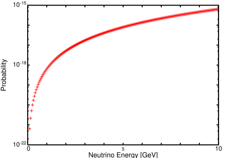
Figure 3: $E_{\nu}$ dependence of the probability Eq. (136) is shown. $B=10$ Tesla is used for the calculation.

they become in the magnetic field

$$P_{B}=6.4\times 10^{-27}\left({B\over B_{0}}\right)^{2}\left({p_{\nu}\over p_{\nu}^{(0)}}\right)^{3},$$ (136)

$$p_{\nu}^{(0)}=10\text{ MeV},\ B_{0}=1\text{ Tesla}.$$

and in the electric field

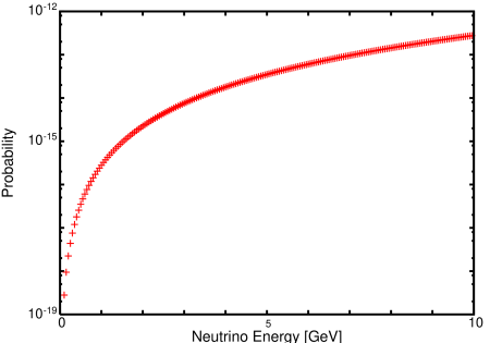
Figure 4: $E_{\nu}$ dependence of the probability Eq. (137) is shown. $E=100$ GV/m is used for the calculation.

$$~{}~{}P_{E}=2.8\times 10^{-20}\left({E\over E_{0}}\right)^{2}\left({p_{\nu}\over p_{\nu}^{(0)}}\right)^{3},$$ (137)

$$p_{\nu}^{(0)}=10\text{ MeV},\ E_{0}=10^{3}\text{ GV/m},$$

Neutrino energy dependences are shown in Figs. 3 ($\nu+B$) and 4 ($\nu+E$).

6.3.2 Low energy neutrinos

The transition probability of the low energy neutrino are

$$P_{B}=4\alpha\left({ecB\over m_{e}c^{2}}\right)^{2}{G_{F}^{2}\over 2}\pi^{-3/2}{1\over\epsilon\sqrt{\sigma_{\gamma}}}p_{\nu}C(m_{\nu}){1\over m_{e}^{2}}$$ (138)

$$P_{E}=4\alpha\left({eE\over m_{e}c^{2}}\right)^{2}{G_{F}^{2}\over 2}\pi^{-3/2}{1\over\epsilon\sqrt{\sigma_{\gamma}}}p_{\nu}C(m_{\nu}){1\over m_{e}^{2}}.$$ (139)

They become in the typical situations

$$\epsilon=10^{-20},\ \sqrt{\sigma_{\gamma}}=10^{-13}\text{ m},p_{\nu}=1\text{ eV},\ E_{0}=10^{3}\text{ GV/m},$$ (140)

$$~{}~{}P_{E}=6.4\times 10^{-38}\left({E\over E_{0}}\right)^{2}.$$

The probabilities Eqs. $(\ref{eq-neu-B-prob}),\ (\ref{high2-E-P}),\text{ and }(\ref{low1-E-P})$ are caused by the overlap of waves on the parent and daughters. The phases of waves become cancelled at small $m_{\gamma}$ or $\epsilon$, and more waves are added constructively then. Thus the effect become larger as they become smaller. The probability shows this and is inversely proportional to $m_{\gamma}^{2}$ or $\epsilon$. They become extremely large as $m_{\gamma}\rightarrow 0$ or $\epsilon\rightarrow 0$.

6.4 Table of processes

The $P^{(d)}$ could be tested in various neutrino processes of wide energy regions.

Neutrino source	Energy	Flux	B	E
Solar neutrino	1–10 MeV	$10^{15}/{{\text{m}}^{2}\text{s}}$	1–5 Tesla	–
Reactor neutrino	3–8 MeV	$10^{20}/{\text{s}}$	1–5 Tesla	–
Cumulonimbus cloud	1–10 MeV	$10^{15}/{{\text{m}}^{2}\text{s}}$(solar $\nu$)	$10^{-5}$ Tesla	$10^{3}$ GV/m
Accelerator neutrino	0.5–50 GeV	$10^{20}$	1–5 Tesla	–
Cosmic neutrino	$\sim 10^{6}$ GeV	$10^{-9}$ GeV/cm2s sr	$10^{-5}$ Tesla	–
Relic neutrino	$1$ meV	$10^{20}/\text{year}$	–	$10^{5}$ GV/m

The diffractive term $P^{(d)}$ becomes substantial in magnitude at high energy or fields. So this process may be relevant to the neutrino of high energy or at high fields, and may give new insights into or measurability of the following processes.

1. The accelerator neutrino has high energy and total intensity of the order $10^{20}$. At $B=10$ Tesla and $P_{\nu}=1(10)$ GeV, we have $P\approx 10^{-18}(10^{-15})$, and using the laser of $E_{0}=10^{3}\text{ GV/m}$ at $P_{\nu}=1(10)\text{ GeV}$, we have $P\approx 10^{-16}(10^{-13})$. The neutrino from the accelerator may be probed by detecting the final gamma rays. For example, at the beam dump of LHC we may set up laser to detect the neutrino interaction.

2. For the reactor neutrino, of the flux $\approx 10^{20}/$s per reactor, a detector of high magnetic field of the order $10$ Tesla, or of high intensity laser, may be able to detect the neutrino.

3. Direct observations of solar neutrinos, which have the energy in $0.5$ MeV to $10$ MeV and flux around $10^{15}$/m² sec, using the detector with strong magnetic field similar to that for axion search [51] would be possible.

4. In Supernova or neutron star, the neutrino photon reaction would give a new important process, because the final photon interacts with matter strongly. As to the detectability of neutrinos from the sun, $10$ GeV is the threshold from the sun, while they from SN interact with $10$ MeV photons.

5. We find that $P^{(d)}$ becomes maximum at $\zeta={\pi\over 2}$ from Eq.$(\ref{non-parallel-low-E})$, and may apply this effect to enhancing the neutrino flux. The term also has the momentum dependence, which may be exploites for “optical” effect of neutrino through the photon interaction.

6. The photon neutrino reaction may be useful for the relic neutrino detection. The reaction rate may be enhanced with such method as the neutrinos mirrors that collect them.[52] We may take advantage of the above effect.

7. The probability becomes huge at extremely high energy. So, this process may be relevant to ultra-high energy neutrino process. [53, 54, 55]),

8. Neutrino may interact with electromagnetic fields in Cumulonimbus cloud.

8-1. Lightening has total energy of the order $900\text{ MJ}\approx 10^{9}$ CV and current $10^{6}$ A in a short period. $cB$ at a radius $r=1\text{ cm}$ is $1.5\times 10^{9}N/C$. Assuming $E=cB=1.5\times 10^{9}$ N/C, and $m_{\gamma}c^{2}=10^{-11}$ eV, $P_{\nu}=10$ MeV we have $P_{E+B}\approx 10^{-15}$. The neutrino inevitably loses its energy, and the photons of the continuous spectrum are emitted. This may be related with the upper-atmospheric lightening [56] .

8-2. The gamma rays observed in Cumulonimbus cloud, [57], may be connected with the diffractive component.

9. Primordial magnetic fluctuations with zero frequency [58] may have interacted with neutrinos before neutrino detachment from the hot neutrino plasma($>$GeV temperature) during the Big Bang. Such signatures may be carried by neutrinos (which is now relic neutrinos).

7 Summary and the future prospect

We have found that the photon interaction expressed by the total derivative Eqs. $(\ref{effective-interaction})$ or $(\ref{neutrino-photon})$, which are derived from the triangle diagram in the standard model, causes the unusual transitions characterized by the time-independent probability. The interaction Lagrangian of this form does not give rise to any physical effect in classical physics, because the equation of motion is not affected. In quantum mechanics, this assertion is correct for the transition rate $\Gamma_{0}$. However, this does not apply to the diffractive term $P^{(d)}$, which manifests the wave characteristics of the initial and final waves. Our results show that $P^{(d)}$ is relevant to experiments and important in understanding many phenomena in nature.

The neutral particles do not interact with the photon in classical mechanics. In quantum field theory, the vacuum fluctuation expressed by triangle diagram gives the effective interaction to the neutral particles such as $1^{+}\text{ meson}\rightarrow\gamma\gamma$ and $\nu+\gamma(B,E)\rightarrow\nu+\gamma$. However, they have vanishing rates due to Landau-Yang-Gell-Mann’s theorem. $P^{(d)}$ does not vanish, nevertheless, and holds unusual properties such as the violation of the kinetic-energy conservation and that of Lorentz invariance. Furthermore the magnitudes become comparable to or even larger than the normal weak processes. Accordingly, the two photon or two gluon decays of the neutral axial vector mesons composed of a pair of electrons or quarks come to have finite decay probabilities. They will be tested in experiments. The neutrino photon processes, which have been ignored, also have finite probabilities from $P^{(d)}$. It will be interesting to observe the neutrino photon processes directly using electric or magnetic fields, or laser and neutrino beams in various energy regions. The diffractive probability $P^{(d)}$ would be also important for understanding the wide neutrino processes in earth, star, astronomy, and cosmology.

The diffractive probability $P^{(d)}$ is caused by the overlap of wave functions of the parent and decay products, which makes the interaction energy finite and the kinetic energy vary. Consequently the final state has continuous spectrum of the kinetic energy and possesses a wave nature unique to the waves. The unique feature of $P^{(d)}$, i.e., independence of on the time-interval $T$, shows that the number of parents, which decrease like $e^{-\Gamma t}$ in the normal decay, is constant now. The state of parent and daughter is expressed by the quasi-stationary states, which is expressed by the superposition of different energies and different from the normal stationary state of the form $e^{-iEt\over\hbar}\psi(x_{i})$.

The probability of the events that the neutrinos or photons are detected is computed with $S[T]$ that satisfies the boundary condition of the physical processes. Applying $S[T]$ we obtained the results that can be compared with experiments. The pattern of the probability is determined by the difference of angular velocities, $\omega=\omega^{E}-\omega^{dB}$, where $\omega^{E}={E_{\nu}/\hbar}$ and $\omega^{dB}={c|\vec{p}_{\nu}|/\hbar}$. The quantity $\omega$ takes the extremely small value ${m^{2}c^{4}}/{(2E\hbar)}$ for light particles such as neutrinos or photons [49] in matter. Consequently, the diffraction term becomes finite in the macroscopic spatial region of $r\leq\frac{2\pi E\hbar c}{m^{2}c^{4}}$.

This allows us to introduce a new class of experimental measurement possibilities of the deployment of photons to detect weakly interacting particles such as neutrinos. Because the modern technology on the electric and magnetic fields and laser, a large number of coherent photons are possible and the effects we have derived may have important implications in detecting and enhancing the measurement of neutrinos with photons. We see a variety of detectability opportunities that have eluded attention till now. These happen either with high energy neutrinos such as from cosmic rays and accelerators; or in high fields (such as intense laser and strong magnetic fields ). In the latter examples, neutrinos from reactors, accelerators, the sun, supernovae, thunder clouds and even polar ice may be detected with enhanced probabilities using intense lasers. We also mention the probability estimate for the primordial relic neutrinos and embedded information in them.

Appendix Appendix A

Wave functions including CG coefficients are

$$\phi_{0}:|J=0,{\vec{P}}=0\rangle=({1\over\sqrt{3}}|1/2,1/2;-1\rangle-{1\over\sqrt{6}}|1/2,-1/2;-1\rangle$$

$$~{}~{}~{}~{}+{1\over\sqrt{6}}|-1/2,1/2;-1\rangle+|-1/2,-1/2;-1\rangle,$$ (A.1)

$$\phi_{1}:|J=1,{\vec{P}}=0\rangle=({1\over\sqrt{2}}|1/2,1/2;0\rangle-{1\over 2}|+1/2,-1/2;-1\rangle$$

$$~{}~{}~{}~{}~{}-{1\over 2}|-1/2,1/2;1\rangle,$$ (A.2)

$$\phi_{2}:|J=2{\vec{P}}=0\rangle=|1/2,1/2;1\rangle.$$ (A.3)

Appendix Appendix B

The integration over a semi-infinite region of satisfying the causality in two dimensional variables, $x_{1}(t_{1},x_{1}),x_{2}(t_{2},x_{2})$

$$I=\int_{\lambda_{1},\lambda_{2}\geq 0}d^{2}x_{1}d^{2}x_{2}{\partial\over\partial t_{1}}{\partial\over\partial t_{2}}f(x_{1}-x_{2})g(x_{1}+x_{2}),$$ (A.4)

where the integrands satisfy

$$g(t_{+},x_{+}=\pm\infty)=0,\ f(t_{-},x_{-}=\pm\infty)=0$$ (A.5)

is made with the change of variables. Due to Eq. (A.5), $I$ would vanish if the integration region were from $-\infty$ to $+\infty$. We write $I$ with variables $x_{+}={x_{1}+x_{2}\over 2},\ x_{-}={x_{1}-x_{2}}$, and have

$$I=I_{1}-I_{2},$$ (A.6)

$$I_{1}=\int_{\lambda_{+}\geq 0}d^{2}x_{-}f(x_{-})d^{2}x_{+}({\partial^{2}\over\partial t_{+}^{2}}g(x_{+})),$$

$$I_{2}=\int_{\lambda_{+}\geq 0}d^{2}x_{+}g(x_{+})d^{2}x_{-}({\partial^{2}\over\partial t_{-}^{2}}f(x_{-})),$$

where $\lambda_{+}=x_{+}^{2}$. It is noted that $x_{+}$ is integrated in the restricted region but $x_{-}$ is integrated in whole region. Thus

$$I_{1}=-\int d^{2}x_{-}f(x_{-})dt_{+}v^{2}({\partial\over\partial x_{+}}g(x_{+}))|_{x_{+}=x_{+,{min}}},$$ (A.7)

$$I_{2}=0,$$

where the functional form $g(x_{+})=g(x_{+}-vt_{+})$ was used. $I$ is computed with the slope of $g(x_{+})$ at the boundary $x_{+}=t_{+}$. We apply this method for computing four dimensional integrals.

Appendix Appendix C

In the case of the low energy region the photon has no effective mass, but is expressed by the index of refraction very close to unity in dilute gas,

$$n=1+\epsilon.$$ (A.8)

Accordingly, the angular velocity in $\bar{\phi}_{c}(\delta t)$ is given by

$$\omega=(1+\epsilon)P_{\gamma}-P_{\gamma}=\epsilon P_{\gamma}.$$ (A.9)

$\epsilon$ in air is

$$\epsilon=0.000292,~{}~{}0C,1~{}\text{atomspheric~{} pressure},$$ (A.10)

and $\epsilon$ in dilute gas becomes extremely small of the order $10^{-14}-10^{-15}$. Consequently the integrand in $P^{(d)}$ is proportional to ${2\over P_{\gamma}\epsilon}$.

Appendix Appendix D Notations :MKSA unit

It is convenient to express the Lagrangian with MKSA unit to study quantum phenomena caused by macroscopic electric and magnetic field [59]. The Maxwell equations for electric and magnetic fields are expressed with the dielectric constant and magnetic permeability of the vacuum, $\epsilon_{0},\mu_{0}$ which are related with the speed of light, c,

$$c={1\over\sqrt{\epsilon_{0}\mu_{0}}}$$ (A.11)

The zeroth component $x_{0}$ in 4-dimensional coordinates $x_{\mu}$, is

$$x_{0}=ct;\ t=~{}\text{sec}.$$ (A.12)

The Maxwell equations in vacuum are,

$${\vec{\nabla}}\cdot{\vec{E}}={1\over\epsilon_{0}}\rho(x),$$ (A.13)

$${\vec{\nabla}}\cdot{\vec{B}}=0,$$

$${\vec{\nabla}}\times({1\over c}{\vec{E}})=-{\partial{\vec{B}}\over\partial x_{0}},$$

$${\vec{\nabla}}\times{\vec{B}}=\mu_{0}{\vec{j}(x)}+{\partial({1\over c}{\vec{E}})\over\partial x_{0}},$$

where the charge density and electric current, $\rho(x),\ {\vec{j}}(x)$, satisfy

$$c{\partial\over\partial x_{0}}\rho(x)+{\vec{\nabla}}{\vec{j}}(x)=0.$$ (A.14)

Using the vector potential

$$A_{\mu}=(A_{0},-{\vec{A}}\,),$$ (A.15)

we write

$${1\over c}{\vec{E}}(x)=-{\partial\over\partial x_{0}}{\vec{A}}(x)-{\vec{\nabla}}A_{0}(x),$$ (A.16)

$${\vec{B}}={\vec{\nabla}}\times{\vec{A}}(x),$$

and the Lagrangian density of electric and magnetic fields

$$L_{EM}=-{1\over 4}{1\over\mu_{0}}F_{\mu\nu}F^{\mu\nu}={\epsilon_{0}\over 2}{\vec{E}}^{2}-{1\over 2\mu_{0}}{\vec{B}}^{2}.$$ (A.17)

The Lagrangian density of electronic fields is,

$$L_{e}=\bar{\psi}(x)\left[\gamma_{0}ic\hbar{\partial\over\partial x_{0}}-\gamma_{l}ic\hbar{\partial\over\partial x_{l}}-mc^{2}\right]\psi,$$ (A.18)

and that of QED is

$$L_{QED}=L_{e}+L_{EM}++ecA_{0}\bar{\psi}\gamma_{0}\psi-ecA_{l}\bar{\psi}\gamma_{l}\psi.$$ (A.19)

Canonical momenta and commutation relations from Eqs. $(\ref{electromagnetic-MKSA})$ and $(\ref{QED-MKSA})$ are

$$\pi_{\psi}(x)={\partial\over\partial\dot{\psi}(x)}L=i\hbar\psi^{\dagger}(x),$$ (A.20)

$$\Pi_{l}(x)(x)={\partial\over\partial\dot{A}_{i}(x)}L={1\over\mu_{0}c^{2}}E_{i},$$

$$\{\psi(x_{1}),\psi^{\dagger}(x_{2})\}\delta(t_{1}-t_{2})=\delta({\vec{x}}_{1}-{\vec{x}}_{2})\delta(t_{1}-t_{2}),$$ (A.21)

$$[A_{i}(x_{1}),\dot{A}_{j}(x_{2})]\delta(t_{1}-t_{2})=i\hbar{1\over\epsilon_{0}}\delta_{ij}\delta({\vec{x}}_{1}-{\vec{x}}_{2})\delta(t_{1}-t_{2}),$$

where the gauge dependent term was ignored in the last equation. Thus the commutation relations for electron fields do not have $\hbar$, and those of electromagnetic fields have $\hbar$ and the dielectric constant $\epsilon_{0}$. ${\hbar\over\epsilon_{0}}$ shows the unit size in phase space. Accordingly the number of states per unit area and the strength of the light-cone singularity are proportional to $1/\epsilon_{0}$. The fields are expanded with the wave vectors as

$$\psi(x)=\sum_{s}\int{d{\vec{k}}\over(2\pi)^{3/2}}({\tilde{\omega}_{0}\over k^{0}({\vec{k}})})^{1/2}(u({\vec{k}},s)b({\vec{k}},s)e^{-ikx}+v({\vec{k}},s)d^{\dagger}({\vec{k}},s)e^{ikx}),$$ (A.22)

$$A_{i}(x)=\sum_{s}\int{d{\vec{k}}\over((2\pi)^{3}2k_{0})^{1/2}}({\hbar\over\epsilon_{0}})^{1/2}(\epsilon_{i}({\vec{k}},s)a({\vec{k}},s)e^{-ikx}+\epsilon^{*}({\vec{k}},s)a^{\dagger}({\vec{k}},s)e^{ikx}),$$ (A.23)

where

$$kx=k_{0}x_{0}-{\vec{k}}{\vec{x}},$$ (A.24)

$$k_{0}({\vec{k}})=\sqrt{{\vec{k}}^{2}+{\tilde{\omega}_{0}}^{2}},~{}~{}\tilde{\omega}_{0}={mc\over\hbar}.$$

The creation and annihilation operators satisfy

$$\{b({\vec{k}}_{1},s_{1}),b^{\dagger}({\vec{k}}_{2},s_{2})\}=\delta({\vec{k}}_{1}-{\vec{k}}_{2})\delta_{s_{1}s_{2}},$$ (A.25)

$$[a({\vec{k}}_{1},s_{1}),a^{\dagger}({\vec{k}}_{2},s_{2})]=\delta({\vec{k}}_{1}-{\vec{k}}_{2})\delta_{s_{1}s_{2}}.$$ (A.26)

The spinor is normalized as

$$\sum_{s}u({\vec{k}},s)\bar{u}({\vec{k}},s)={{\gamma}\cdot k+\tilde{\omega}_{0}\over 2\tilde{\omega}_{0}},$$ (A.27)

and the light-cone singularity is

$$\Delta_{+}(x_{1}-x_{2})=\int{d{\vec{k}}\over(2\pi)^{3}2k_{0}}e^{-ik\cdot(x_{1}-x_{2})}=2i{1\over 4\pi}\delta(\lambda)\epsilon(\delta x^{0})+\cdots,$$ (A.28)

where the less-singular and regular terms are in $\cdots$.

The action

$$S=\int dx(L_{QED}+\bar{\psi}(x)\gamma_{\mu}(1-\gamma_{5})\psi(x)J^{\mu}(x)),$$ (A.29)

$$J^{\mu}(x)={G_{F}\over\sqrt{2}}\bar{\nu}(x)\gamma^{\mu}(1-\gamma_{5})\nu(x).$$

governs the dynamics of electron, photon and neutrino. Integrating $\psi(x)$ and $\bar{\psi}(x)$, we have $\text{Det}(D+J^{\mu}\gamma_{\mu}(1-\gamma_{5}))$ and the effective action between neutrino and photon

$$S_{eff}={e^{2}\over 8\pi^{2}c\hbar^{2}}f(0)\int dx{\partial\over\partial x_{\nu}}\left[J^{\nu}(x)\epsilon_{\alpha\beta\rho\sigma}{\partial\over\partial x_{\alpha}}A^{\beta}{\partial\over\partial x_{\rho}}A^{\sigma}\right],$$ (A.30)

where

$$f(0)={1\over 2{\tilde{\omega}_{0}}^{2}}.$$ (A.31)

The magnetic field and electric field in the 3-rd direction, and laser field expressed by the external fields,

$$F^{\mu\nu}_{ext}=\epsilon^{03\mu\nu}B,\ F^{\mu\nu}_{ext}=\epsilon^{12\mu\nu}{E\over c},\ A^{\mu}_{laser}(x)$$ (A.32)

are substituted to the action Eq .$(\ref{action-MKSA})$, and we have the actions

$$S_{eff,B}=g_{B}\epsilon_{03\rho\sigma}\int dx{\partial\over\partial x_{\nu}}[\bar{\nu}(x)\gamma^{\nu}(1-\gamma_{5})\nu(x){\partial\over\partial x_{\rho}}A^{\sigma}(x)],$$ (A.33)

$$S_{eff,E}=g_{E}\epsilon_{12\rho\sigma}\int dx{\partial\over\partial x_{\nu}}[\bar{\nu}(x)\gamma^{\nu}(1-\gamma_{5})\nu(x){\partial\over\partial x_{\rho}}A^{\sigma}(x)],$$ (A.34)

$$S_{eff,laser}=g_{l}\epsilon_{\mu\nu\rho\sigma}\int dx{\partial\over\partial x_{\nu}}[\bar{\nu}(x)\gamma^{\nu}(1-\gamma_{5})\nu(x)F^{\mu\nu}_{laser}(x){\partial\over\partial x_{\rho}}A^{\sigma}(x)],$$ (A.35)

where the coupling strengths are

$$g_{B}={e^{2}\over 8\pi^{2}c\hbar^{2}}f(0)B{G_{F}\over\sqrt{2}},$$ (A.36)

$$g_{E}={e^{2}\over 8\pi^{2}c\hbar^{2}}f(0){E\over c}{G_{F}\over\sqrt{2}},$$ (A.37)

$$g_{l}={e^{2}\over 8\pi^{2}c\hbar^{2}}f(0){G_{F}\over\sqrt{2}}.$$ (A.38)

The wave vectors are connected with the energy and momentum

$$E({\vec{k}})=\hbar ck_{0}({\vec{k}}),\ {\vec{p}}=\hbar c{\vec{k}}.$$ (A.39)

Appendix Appendix E Integration formulae

The integrals

$$I_{0}=\int_{\lambda_{+}=0}d^{4}x_{1}d^{4}x_{2}\rho_{s}(x_{-}^{0})({\partial\over\partial x_{+}^{0}})^{2}e^{-\chi(x_{1})-\chi(x_{2})^{*}}\delta((\lambda_{-})^{2})e^{ip\cdot x_{-}},$$ (A.40)

$$I_{i}=\int_{\lambda_{+}=0}d^{4}x_{1}d^{4}x_{2}\rho_{s}(x_{-}^{0})({\partial\over\partial x_{+}^{i}})^{2}e^{-\chi(x_{1})-\chi(x_{2})^{*}}\delta((\lambda_{-})^{2})e^{ip\cdot x_{-}},$$ (A.41)

$$\rho_{s}(x_{-}^{0})=1+i{x_{1}^{0}-x_{2}^{0}\over E\sigma_{\gamma}},$$

where the spreading in the transverse direction in Eq. (58) leads to $\rho_{s}(x_{-}^{0})$ in the right hand sides. Changing the variables to $x_{+}$ and $x_{-}$, we have

$$\chi(x_{1})+\chi(x_{2})^{*}=\chi^{(+)}(x_{+})+\chi^{(-)}(x_{-})+\chi^{(+-)}(x_{+},x_{-}),$$ (A.42)

$$\chi^{(+)}(x_{+})={1\over\sigma_{\gamma}}(({x_{+,l}}-v(x_{+,0}))^{2}+{1\over 2\sigma_{T}(+)}(({\vec{x}}_{+})_{T}^{2}),$$

$$\chi^{(-)}(x_{-})={1\over 4\sigma}_{\gamma}({x_{-,l}}-v(x_{-,0}))^{2}+{1\over 8\sigma_{T}(+)}(({\vec{x}}_{-})_{T}^{2}),$$

$$\chi^{(+-)}(x_{+},x_{-})={1\over\sigma_{T}(-)}(({\vec{x}}_{+})_{T}({\vec{x}}_{-})_{T}),$$

where the wavepacket sizes in the transverse direction are

$${1\over 2\sigma_{T}(+)}={1\over 2\sigma_{T}(1)}+{1\over 2\sigma_{T}(2)^{*}},$$ (A.43)

$${1\over 2\sigma_{T}(-)}={1\over 2\sigma_{T}(1)}-{1\over 2\sigma_{T}(2)^{*}}.$$

The wavepacket expands in the transverse direction and the size $\sigma_{T}(+)$ is given by

$$\sigma_{T}(+)={\sigma_{\gamma}\over 2}-{i\over 4E}(x_{-}^{0})+O(x_{-}^{2},x_{+}^{2}).$$ (A.44)

The off-diagonal term $\chi(x_{+},x_{-})$ gives small corrections and is ignored. We have

$$I_{0}={1\over\sigma_{\gamma}}I_{0}(+)I(-),$$ (A.45)

$$I_{0}(+)=\int_{x_{+}^{0}=|{\vec{x}}_{+}|}dx_{l}^{+}d^{2}{\vec{x}}_{T}^{+}e^{-\chi(x_{+})}{({\vec{x}}_{T}^{+})^{2}\over x_{l}^{+}}=\int dx_{+}^{l}\pi(2\sigma_{T}(+))^{2}{1\over x_{+}^{l}},$$

$$I(-)=\int d^{4}x_{-}\rho(x_{-}^{0})e^{-\chi(x_{-})}\delta(\lambda_{-}^{2})e^{ipx_{-}}=\int dx_{-}^{0}\rho(x_{-}^{0}){4\sigma_{T}(+)\over x_{-}^{0}}e^{i\omega x_{-}^{0}},$$

and

$$I_{0}=\pi\int_{0}^{T}dx_{+}^{l}{1\over x_{+}^{l}}\int_{-x_{+}^{l}}^{+x_{+}^{l}}dx_{-}^{0}\rho(x_{-}^{0}){16\sigma_{T}(+)^{3}\over\sigma_{l}}{e^{i\omega x_{-}^{0}}\over x_{-}^{0}}$$

$$=-i2\pi^{2}(\sigma_{\gamma}^{2}\text{log}(\omega T)+{\sigma_{\gamma}\over 4\omega E}).$$ (A.46)

Eq. $(\ref{log-constant})$ is composed of the $\log T$ term and constant. At $\omega\approx 0$, the latter is important and at a larger $\omega$, the former is important.

Similarly

$$I_{i} =I_{i}(+)I(-)$$ (A.47)

$$I_{i}(+) =\int_{x_{+}}^{i}=\pm\sqrt{(x_{+}^{0})^{2}-(x_{+}^{l})^{2}-(x_{+}^{i})^{2}}dx_{+}^{0}dx_{+}^{l}d{\vec{x}}_{+}^{i^{\prime}}{x_{+}^{i}\over\sigma_{T}(+)}e^{-\chi(x_{+})}$$

$$=\pi\int dx_{+}^{0}{2\sigma_{T}(+)\over x_{+}^{0}},$$

and

$$I_{i}=\pi\int_{0}^{T}dx_{+}^{0}{1\over x_{+}^{0}}\int_{x_{+}^{0}}^{x_{+}^{0}}dx_{-}^{0}\rho(x_{-}^{0})8\sigma_{T}(+)^{2}{e^{i\omega x_{-}^{0}}\over x_{-}^{0}}$$

$$=-i2\pi^{2}(\sigma_{\gamma}^{2}\text{log}(\omega T)).$$ (A.48)

In high energy regions, $\omega={m_{\gamma}^{2}\over 2E}$, and

$$I_{0}=-i2\pi^{2}(\sigma_{\gamma}^{2}\text{log}(\omega T)+{\sigma_{\gamma}\over 4m_{\gamma}^{2}}),$$ (A.49)

$$I_{T,i}=-i2\pi^{2}(\sigma_{\gamma}^{2}\text{log}(\omega T)),$$ (A.50)

$$I_{l}=I_{0}.$$ (A.51)

In low energy regions, $\omega=\epsilon p$, and

$$I_{0}=-i2\pi^{2}(\sigma_{\gamma}^{2}\text{log}(\omega T)+{\sigma_{\gamma}\over 4\epsilon p^{2}}),$$ (A.52)

$$I_{i}=-i2\pi^{2}(\sigma_{\gamma}^{2}\text{log}(\omega T)),$$ (A.53)

$$I_{l}=I_{0}.$$ (A.54)

References

- [1] K. Ishikawa and Y. Tobita. Prog. Theor. Exp. Phys. 073B02, doi:10.1093/ptep/ptt049 (2013).
- [2] K. Ishikawa and Y. Tobita. Ann of Phys, 344, 118(2014), doi: 10.1016/j.aop.2014.02.007.
- [3] J. J. Sakurai, Advanced quantum mechanics (Princeton University Press, New Jersey 1979) p.184.
- [4] R. Peierls. Surprises in Theoretical Physics (Princeton University Press, New Jersey 1979) p.121.
- [5] W. Greiner, QUANTUM MECHANICS An Introduction (Springer, New York Berlin Heidelberg, 1994), p282.
- [6] P. A. M. Dirac. Pro. R. Soc. Lond. A 114, 243 (1927).
- [7] L. I. Schiff. Quantum Mechanics (McGRAW-Hill Book COMPANY,Inc. New York, 1955).
- [8] M. L. Goldberger and Kenneth M. Watson, Collision Theory (John Wiley & Sons, Inc. New York, 1965).
- [9] R. G. Newton, Scattering Theory of Waves and Particles (Springer-Verlag, New York, 1982).
- [10] J. R. Taylor, Scattering Theory: The Quantum Theory of non-relativistic Collisions (Dover Publications, New York, 2006).
- [11] M. Iinuma,et al, Phys.Letters A 346 255-260(2005)
- [12] H. Lehman, K. Symanzik, and W. Zimmermann, Il Nuovo Cimento (1955-1965) 1, 205 (1955).
- [13] F. Low, Phys. Rev. 97, 1392 (1955).
- [14] K. Ishikawa and T. Shimomura, Prog. Theor. Phys. 114, 1201 (2005) [hep-ph/0508303].
- [15] K. Ishikawa and Y. Tobita. Prog. Theor. Phys. 122, 1111 (2009) [arXiv:0906.3938[quant-ph]].
- [16] K. Ishikawa and Y. Tobita, AIP Conf. proc. 1016, 329(2008); arXiv:0801.3124 [hep-ph].
- [17] K. Ishikawa and Y. Tobita, arXiv:1106.4968[hep-ph].
- [18] B. Kayser. Phys. Rev. D24, 110 (1981).
- [19] C. Giunti, C. W. Kim and U. W. Lee. Phys. Rev. D44, 3635 (1991).
- [20] S. Nussinov. Phys. Lett. B63, 201 (1976).
- [21] K. Kiers, S. Nussinov and N. Weiss. Phys. Rev. D53, 537 (1996) [hep-ph/9506271].
- [22] L. Stodolsky. Phys. Rev. D58, 036006 (1998) [hep-ph/9802387].
- [23] H. J. Lipkin. Phys. Lett. B642, 366 (2006) [hep-ph/0505141].
- [24] E. K. Akhmedov. JHEP. 0709, 116 (2007) [arXiv:0706.1216 [hep-ph]].
- [25] A. Asahara, K. Ishikawa, T. Shimomura, and T. Yabuki, Prog. Theor. Phys. 113, 385 (2005) [hep-ph/0406141]; T. Yabuki and K. Ishikawa. Prog. Theor. Phys. 108, 347 (2002).
- [26] H. L. Anderson et al. Phys. Rev. 119, 2050 (1960).
- [27] K. Homma, D. Habs, and T. Tajima, Appl. Phys. B106, 229(2012).
- [28] T. Tajima, and K. Homma, Int. J. Mod. PhysA27,1230027(2012).
- [29] C. H. Lai, Ph.D dissertation (Univeristy of Texas,Austin,1994); T. Tajima and K. Shibata, ”Plasma Astrophysics” (Addison-Wesley,Reading,1997) p.451.
- [30] L. Landau. Sov. Phys. Doclady 60, 207(1948).
- [31] C. N. Yang. Phys. Rev. 77, 242(1950).
- [32] H. Fukuda and Y. Miyamoto, Prog. Theor. Phys.4,49(1949).
- [33] J. Steinberger, Phys. Rev. 76, 1180(1949).
- [34] L. Rosenberg. Phys. Rev. 129, 2786(1963).
- [35] S. L. Adler. Phys. Rev. 177, 2426(1969).
- [36] J. Liu, Phys. Rev. D44, 2879(1991).
- [37] R. P. Feynman, Phys. Rev. 76, 749(1949).
- [38] A. I. Alelseev, Zh. Eksp. Teor. Fiz. 34,1195(1958) [Sov Phys. JETP 7,826(1958)].
- [39] K. A. Tumanov, Zh. Eksp. Teor. Fiz. 25, 385(1953).
- [40] T. Tajima and J. M. Dawson, Phys. Rev. Lett. 43, 267(1979).
- [41] R. Barbieri, R. Gatto, and R. Kogerler, Phys. Lett. 60B, 183(1976).
- [42] W. Kwong,P. B. Mackenzie, R. Rosenfeld, and J. L. Rosner, Phys. Rev. D37,3210(1988).
- [43] Z. P. Li, F.E.Close, and T.Barns, Phys. Rev. D43, 2161(1991).
- [44] G.T. Bodwin, E. Braaten and G. P. Lepage, Phys. Rev. D51, 1125(1995).
- [45] Han-Wen Huang and Kuang-Ta Chao, Phys. Rev. D54, 6850(1996).
- [46] J. E. Gaiser, et al, Phys. Rev. D34, 711(1986).
- [47] S. B. Athar, et al, Phys. Rev. D70, 112002(2004).
- [48] M. Ablikin, et al, Phys. Rev. D71, 092002(2005).
- [49] J. Beringer et al. [Particle Data Group], J. Phys.Rev D86, 010001(2012).
- [50] M. Gell-Mann. Phys. Rev. Lett. 6, 70(1961).
- [51] Y. Inoue, et. al, Phys. Lett. B668, 93(2008).
- [52] J.Arafune and G.Takeda, “Total Reflection of Relic Neutrinos from Material Targes”, University of Tokyo, ICEPP Report, ut-icepp 08-02, and private communication.
- [53] M. G. Aartsen et al. (IceCube Collaboration): Observation of High-Energy Astrophysical Neutrinos in Three Years of IceCube Data, 2014, arXiv:1405.5303 [astro-ph.HE].
- [54] P. Abreu et al. (Pierre Auger Collaboration), Adv. High Energy Phys. 2013, 708680 (2013), arXiv:1304.1630 [astro-ph.HE].
- [55] G. I. Rubtsov et al. (Telescope Array Collaboration), J. Phys. Conf. Series 409 (2013), 012087.
- [56] R. C. Franz, R. J. Nemzek, and J. R. Winckler, Science 249 48 (1990); G. J. Smith, et.al., Science,textbf264,1313(1994).
- [57] T.Torii, M.Takeishi, and T. Hosono, J.Geophys.Res.107,4324(2002); H.Tsuchiya, et. al, Phys.Rev.Letters. 99165002(2007)
- [58] T.Tajima, S. Cable, K.Shibata, and R. M. Kulsrud, Ap. J. 390, 309 (1992).
- [59] Claude Cohen-Tannoudji, Jacques Dupont-Roc, and Gilbert Grynberg. Photons and atoms: Introduction to Quantum Elctrodynamics (John Wiley & Sons, Inc. New York, 1989).