Role of the potential landscape on the single-file diffusion through channels

Abstract

Transport of colloid particles through narrow channels is ubiquitous in cell biology as well as becoming increasingly important for microfluidic applications or targeted drug delivery. Membrane channels in cells are useful models for artificial designs because of their high efficiency, selectivity and robustness to external fluctuations. Here we model the passive channels that let cargo simply diffuse through them, affected by a potential profile along the way. Passive transporters achieve high levels of efficiency and specificity from binding interactions with the cargo inside the channel. This however leads to a paradox: why should channels which are so narrow that they are blocked by their cargo evolve to have binding regions for their cargo if that will effectively block them? Using Brownian dynamics simulations, we show that different potentials, notably symmetric, increase the flux through narrow passive channels – and investigate how shape and depth of potentials influence the flux. We find that there exist optimal depths for certain potential shapes and that it is most efficient to apply a small force over an extended region of the channel. On the other hand, having several spatially discrete binding pockets will not alter the flux significantly. We also explore the role of many-particle effects arising from pairwise particle interactions with their neighbours and demonstrate that the relative changes in flux can be accounted for by the kinetics of the absorption reaction at the end of the channel.

I Introduction

Transport of macromolecules through nano-sized pores and narrow protein channels is essential for cell function alberts2008molecular while also becoming increasingly important in microfluidic applications shah2008 ; Pagliara2013 or to understand drug delivery.Sugano2010 Channels in cell membranes are remarkable for their high efficiency, selectivity and robustness with respect to fluctuations of their environment hille2001ion and come in two flavours. Active transporters move their cargo by using cellular energy, e.g. from hydrolysing adenosine triphosphate or by harvesting concentration gradients of cell metabolites across the membrane. On the other hand, passive transporters are driven by the growth of entropy of the system as they translocate their specific cargo. Initially thought of as molecular sieves that select via the pore size to let the ‘right’ cargo simply diffuse through the channel, it is now well established that passive transporters achieve high levels of efficiency and specificity from binding interactions with the cargo inside the channel. A well-characterised example is the bacterial channel Maltoporin, where oligosaccharide transport is facilitated by an extended binding region.Schirmer1995 Although many more examples of this phenomenon have since been discovered using a plethora of methods (e.g. ex-situ crystallographic studies,Kasianowicz2006 indirect measurements of ionic currents Hilty2001 and molecular dynamics simulations,Jensen2002 ) the exact details of the mechanisms of passive transporters are still poorly understood.Kolomeisky2007

Our work is motivated by a seeming paradox that arises when one considers the flux through a narrow channel, such as Maltoporin, which prevents particles from overtaking each other. Increasing the binding affinity between the channel interior and the cargo will prolong the time each particle spends inside the channel, hence reducing the flux and effectively blocking it. Why then would channels evolve to have binding regions for the molecules they have evolved to translocate? In this paper, we combine the results of Brownian dynamics simulations with theoretical arguments to show how developing binding regions inside a channel can indeed increase flux through narrow channels. We model the binding regions using a variety of potential-energy landscapes along the channel and investigate the dependence of the flux through the channel on the shape and depth of these potentials.

We first consider a single freely diffusing particle to tune our Brownian dynamics simulations in the setting where an exact analytical solution for the transport exists, applying various tests to the simulation procedure to ensure its proper reflection of the physical situation. We then investigate single-file diffusion through a channel to analyse the dependence of particle flux on the shape and depth of applied potentials. Finally, we demonstrate that we can account for the relative changes in flux by considering the diffusion-limited reaction kinetics of the absorption in a scheme Dorsaz2010 based on the osmotic pressure along the channel alone.

To investigate the dynamics of colloid particles diffusing freely or in a potential, we need to solve the Langevin or corresponding Fokker-Planck equation. In a many-body problem like the one considered here, solving these equations directly is completely unfeasible and we therefore turned to Brownian dynamics (BD) simulations Chen2004 using the LAMMPS package.Plimpton1995 This allowed us to efficiently compute solutions of the equations from an ensemble of simulated stochastic processes with the same initial conditions.

II Free Brownian particle

The one-dimensional motion of a Brownian particle is described by the Langevin equation $m\dot{v}+\alpha v=\zeta(t)$, where $m$ is the particle mass, $v$ its velocity and $\alpha$ is the viscous drag coefficient. We further assume white noise $\zeta(t)$ with $\langle\zeta(t)\zeta(t^{\prime})\rangle=\Gamma\delta(t-t^{\prime})$, where $\Gamma=2\alpha k_{B}T/m$ is the intensity of the stochastic force, satisfying the fluctuation-dissipation theorem. The general solution for the root mean square displacement of the particle is Uhlenbeck1930 :

$$\langle\Delta x^{2}\rangle=\frac{2k_{B}T\,m}{\alpha^{2}}\left(t/\tau_{v}-1+\exp(-t/\tau_{v})\right)$$ (1)

with the velocity relaxation time $\tau_{v}=m/\alpha$. In the overdamped (or diffusive) regime, with $t\gg\tau_{v}$, we recover the Einstein result: $\langle\Delta x^{2}\rangle=2({k_{B}T}/{\alpha})t$, where one defines the diffusion constant $D\equiv k_{B}T/\alpha$. On the other hand, in the inertial regime $t\ll\tau_{v}$, the displacement grows linearly with time: $\langle\Delta x^{2}\rangle=({k_{B}T}/{m})t^{2}$.

Brownian dynamics simulation

To verify that LAMMPS yields particle trajectories with the right statistical properties, we first simulated freely diffusing spherical Brownian particles of different sizes at different temperatures. The goal was to identify the crossover from the inertial to the diffusive regime at different temperatures and to verify the fluctuation-dissipation theorem.

Integration of the Langevin equation and the application of thermostat conditions was done via the fix_langevin routine.Schneider1978 The free particles were simulated in a box with periodic boundary conditions and were assigned initial velocities drawn from a uniform distribution for the given temperature. The viscous drag coefficient $\alpha$ was computed using Stoke’s law for a spherical particle at low Reynolds number: $\alpha=6\pi\eta R$ where $R=\sigma/2$ is the particle radius and $\eta$ is the fluid viscosity.

Figure 1: Inertial to diffusive crossover for the single particle. Points are rms displacements computed from the simulated trajectories of 100 freely diffusing single particles for each set of parameters. Solid lines are the inertial and the diffusive limits of the Langevin equation solution (1). Particle #2 initially follows the trajectory of particle #3, with has the same mass, before crossing over to the trajectory of particle #1, which has the same drag coefficient. Errors were computed from the statistical distribution of particle displacements, but are to small to appear on this scale.

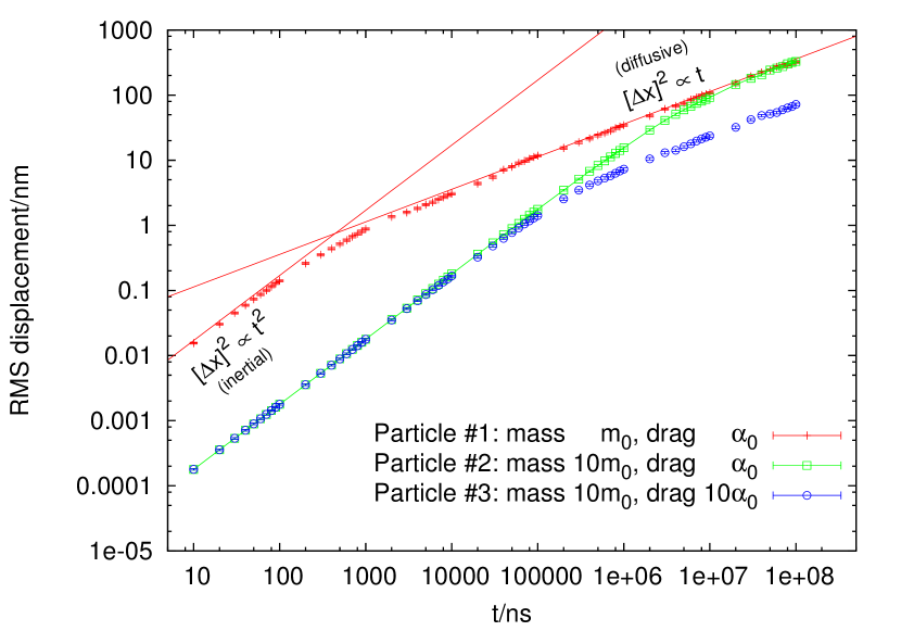
Figure 1 shows the average root mean squared displacement of the particles computed as the average of 100 simulated trajectories per particle. Since there is no energy scale for the free particle, we used natural units and in this case set the diameter of the particles to $\sigma=1\mu\text{m}$ and their mass density to that of water, yielding a mass of $m\sim 4.2\cdot 10^{-15}\text{kg}$. We found that the statistical relative errors for the average trajectories were negligible for this number of simulations.

The crossover time was determined by inspection from the graphs. We can read off a crossing-over time of $\sim 0.5\mu\text{s}$ for particle #3 where the inertial response has fully died down; this is on the same order as the characteristic time scale $\tau_{v}=m/\alpha\sim 220\text{ns}$.

We simulated particles of different sizes ($1-20\mu\text{m}$) at different temperatures ($293-400\text{K}$). Here it may be necessary to account for the fluid viscosity variation with temperature, and we used the empirical formula for water Al-Shemmeri2012 :

$$\eta(T)=2.141\cdot 10^{-5}\cdot 10^{247.8/(T-140)}.$$ (2)

We have confirmed that the particle trajectories generated by LAMMPS had the statistical properties expected from theory. We were also able to confirm that the crossover time $\tau_{v}$ is practically independent on the heat bath temperature, since the viscosity only depends weakly on temperature in the range that we covered in our simulations.

Figure 2: Testing the fluctuation-dissipation theorem. Diffusion constants $D_{sim}$ were obtained from of average trajectories and are plotted as points, multiplied by the drag coefficient $\alpha=6\pi\eta\sigma$ which was given as a parameter to the fix_langevin routine for simulations at different temperatures. The different colours correspond to the types of particles, with different radii as indicated on the plot. The corresponding Einstein relations $D\alpha=k_{B}T$ are plotted as solid lines.

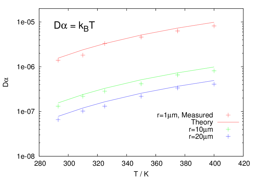
To verify the fluctuation-dissipation theorem, which is used to derive the Einstein relation $D=k_{B}T/\alpha$, we computed the diffusion constant from a linear fit of the last three decades of each trajectory, i.e. for $t>10^{5}\text{ns}$, obtained from 100 simulated particles using the SciPy Oliphant2007b curve_fit routine. Figure 2 shows the product $D\alpha$ that was computed theoretically using the Stokes relation (see above) as a function of temperature, compared with the measured data. The predicted trend is observed, with a very small systematic offset that has been observed for a number of integration schemes in Brownian dissipative dynamics.Vattulainen2002 Essentially, this is an artefact that arises from the coarse-graining of the microscopic properties of the fluid using a random force $\zeta$ while imposing overall momentum conservation; this error is not significant for our purposes for two reasons: the algorithm produces trajectories in almost perfect agreement with the theory across a broad range of temperatures and furthermore, previous studies have shown that the effects due to integrator artefacts are only significant when the conservative forces of interest are comparable to the thermal fluctuations Vattulainen2002 – all the potentials we apply will exceed energies of a few $k_{B}T$.

III Free particle in a channel

Having established the dynamics of Brownian particles and verified that LAMMPS generates trajectories with the desired statistics, we now turn our attention to the diffusion of free particles confined in a narrow channel.

We considered particles of diameter $\sigma=2R$ freely diffusing through a channel of radius $\sigma$. Note that from here on, we will use Lennard-Jones (LJ) units which render all quantities dimensionless by assuming that particle interactions follow the standard Lennard-Jones potential $V(r)=4\epsilon[(\sigma/r)^{12}-(\sigma/r)^{6}]$ and setting the particle mass $m$, the Boltzmann constant $k_{B}$ and $\epsilon$ and $\sigma$ as defined above equal to 1 ljunits . All masses are to be understood as multiples of these fundamental values, while other variables can be transformed to a dimensionless form by a scaling with an appropriate combination of the above, e.g. for time: $t_{\mathrm{LJ}}=t\cdot\sqrt{\epsilon m^{-1}\sigma^{-2}}$. For a full list of conversion formulae see.ljunits LJ units are widely used in computational physics and offer the advantage of being able to treat systems of different size and energy scales in one framework.

In our simulations, particles are modelled as spheres with a Lennard-Jones 12/6 type repulsion and no attractive interaction tail, that is, the LJ potential of pair interaction is truncated at the point of its minimum, $r^{*}=2^{1/6}\sigma$. The channel radius is too small to allow particles to overtake each other, thus producing the single-file diffusion and reflecting the experimental fact that many metabolites will completely block their channels during the transport due to their tight fit.Nestorovich2002

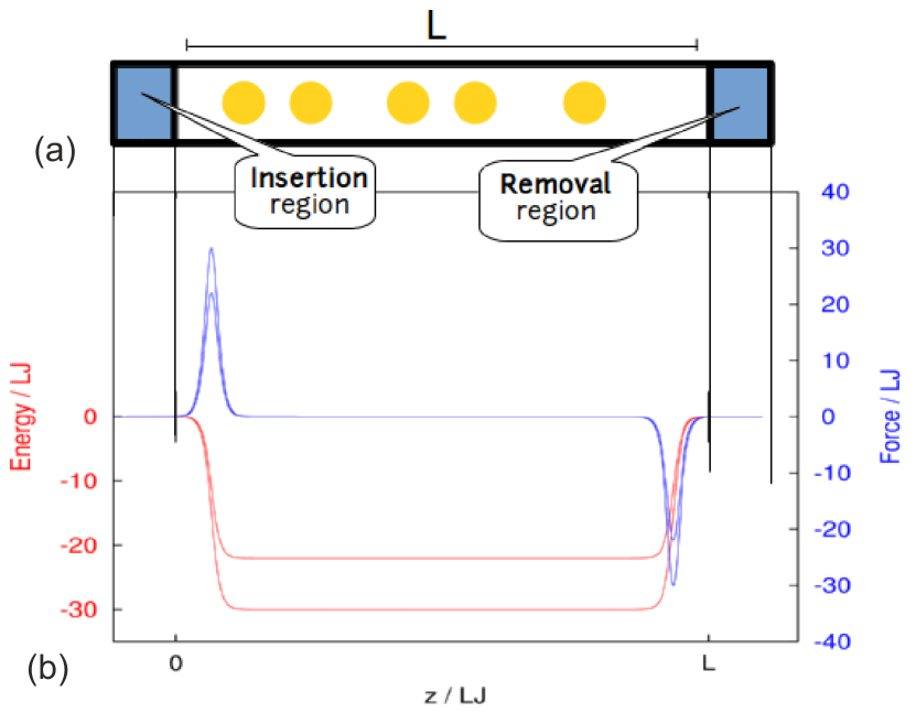
Figure 3(a) shows a 2D-projection of the setup of the simulation box (all simulations were carried out in full three dimensions). The ‘channel’ of length $L$ is the white area in the middle and is aligned along the $z$-axis. Its walls interact with particles using the repulsive part of the Lennard-Jones potential, same as described above, thereby ‘softly’ preventing contact. Particles are inserted in the insertion region to the left (blue) if there is enough space. They then diffuse inside the cylinder. Once they have crossed the channel and entered the removal region to the right of the channel (blue), they are removed from the simulation. Underneath, in Fig. 3(b) is a plot of two example potentials $V(z)$ and their corresponding force landscapes, to scale. To investigate the first passage time distribution, no potential was applied.

Figure 3: Channel geometry and an applied potential. (a) The simulation box is split in three, with the ‘channel’ of length $L$ in the middle aligned along the z-axis, containing spherical particles. Particles are inserted in the blue region to the left and removed from the simulation once they have crossed the channel and entered the blue removal region to the right. (b) A typical applied potential (red), in this case a uniform well, and the corresponding force exerted on a particle (blue), to scale.

Distribution of first passage times

To check the physics of our channel setup, we looked at the distribution of first passage times, $f(\tau)$, of particles freely diffusing through the channel, i.e. without any applied potential. There is a classical result due to Lord Kelvin, obtained by the methods of images Lappala2013 – however, it is only applicable when the particle is free to diffuse as far as necessary to the left of $z=0$, while the first passage time is being tested by arriving at $z=L$ to the right of its entry point, see Fig. 3(a). In our case the passage is blocked to the left, so to find the probability for a particle $p(z,t)$ one needs to solve the one-dimensional free diffusion equation with the boundary conditions: reflective wall, $\nabla p=0$ at $z=0$, absorbing wall, $p=0$ at $z=L$, and the initial condition for insertion: $p(x,t=0)=\delta(z)$. The solution is:

$$p(z,t)\propto\sum_{n=0}^{\infty}\cos\left[\frac{\pi z}{L}(n+1/2)\right]\exp\left(-\frac{\pi D^{2}(n+1/2)^{2}}{L^{2}}t\right),$$ (3)

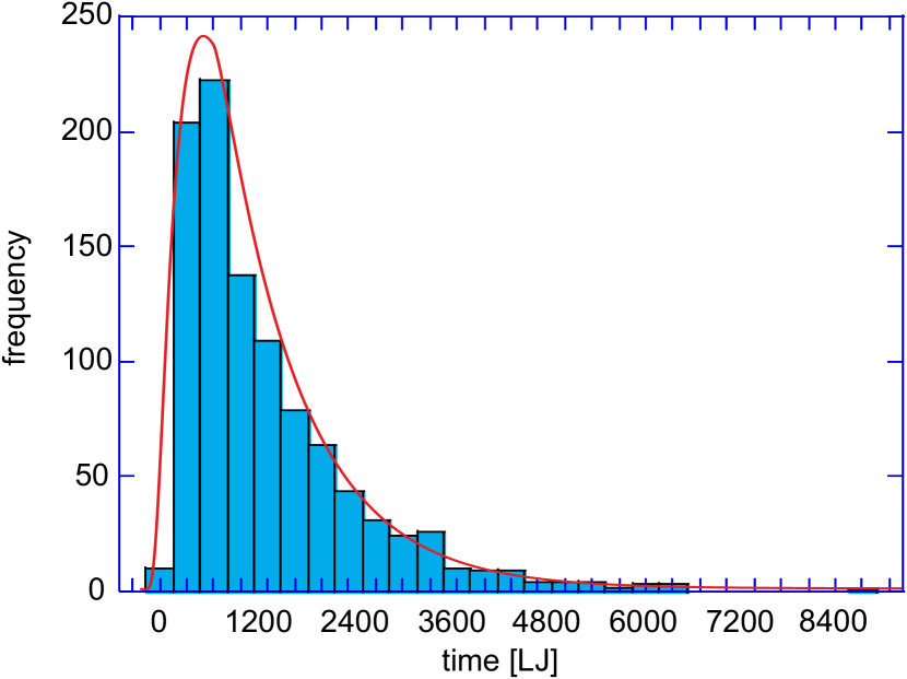
where the constant $C_{0}$ is determined by normalisation. The survival probability for the particle to remain anywhere between 0 and $L$, having started at $z=0$ is obtained by integration: $Q(t)=\int_{0}^{L}p(x,t)dx$. Given the boundary conditions, $Q(t)$ does not depend on anything happening outside the $(0-L)$ interval. Given the definition of the survival probability, the fraction of particles equal to $-dQ(t)/dt$ is absorbed between $t$ and $t+dt$. This means that $f(t)=-dQ(t)/dt$ is actually the probability density of the time $t$ that takes the particle to reach $z=L$ for the first time. This distribution function is plotted in Fig.4, and it gives average first passage time $\tau_{\text{diff}}\approx 4.92L^{2}/\pi^{2}D$.

We measured the passage times in 500 simulations of a single particle diffusion (to ensure no pair-interaction events could take place), where we inserted a particle in the insertion area and allowed it to freely diffuse to the end of the channel, the time for which we measured. We fit the distribution of first passage times to the resulting histogram of particle travel times in Fig.4, where only the diffusion constant $D$ and a normalisation act as fitting parameters. The data are in good agreement with the model, and we find a bare diffusion constant $D_{0}=0.28$.

Figure 4: Distribution of first passage times for free diffusion. The histogram was obtained from the first passage time of 500 single-particle simulations. The solid line is the theoretically calculated distribution $f(\tau)$, fitted using the diffusion constant $D=0.284$ and a normalisation constant as the fitting parameters.

Interestingly, we found that when we considered a similar experiment where we inserted several particles into the channel one by one at a certain low frequency, the distribution of first passage times severely deviated from the free-diffusion result even at concentrations of just 2-3 particles inside a channel of length $L=30$ at any one time. This shows that many-particle effects caused by particle-particle interactions cannot realistically be ignored even at the lowest of concentrations, a point to which we will return at the end of this paper. In this particular case, the average first passage time was significantly increased at these concentrations, suggesting a smaller diffusion constant or higher effective resistance.

IV Potential along the channel

Having established that our simulation setup produces physically meaningful results, we now turn to the dependence of the flux through a passive channel on the potential landscape inside it. We therefore made a series of experiments, in each of which we simulated the insertion of 100 particles in the channel at a rate $0.001\tau^{-1}=1/T_{\text{in}}$. Since this is now a genuine multi-particle problem, simulation time increases accordingly. We therefore made use of the parallel computing capacities of LAMMPS.

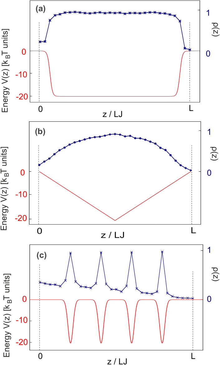
Particles were only inserted if there was enough space in the insertion region; if a particle could not be inserted due to crowding at the channel entry, the insertion was skipped and the next attempt was made after a time interval of $T_{in}$. Inside the channel, one out of a number of different potential shapes was applied with potential depth between $V_{\text{min}}\in[-5,-70]$ in LJ units. The shapes of the potential are shown in the insets of Fig. 6. Note that potential ‘steps’ are modelled using $\tanh$ functions, hence the names ‘Double tanh’ etc. Potential shapes include ‘continuous’ potentials, where the channel is modelled having a homogeneous attractive interaction along its entire length (single/double tanh, triangular potentials) or ‘discrete’ potentials, where the channel provides a number of discrete, spatially well-defined binding pockets, modelled as a Gaussian with a depth $V_{\text{min}}$ and a standard deviation of $0.5\sigma$.

Figure 5: Example trajectory of a single particle in a channel with four binding pockets. Time is plotted on the y-axis and displacement along the channel in red on the x-axis. The potential inside the channel (blue) has four binding pockets, and the trajectory clearly displays trapping of the particle in every pocket, spending most time in the second pocket. The overall flux, however, is unaltered compared to a channel with no potential at all (see Figs. 6 and 7).

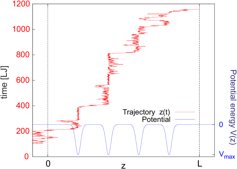
Despite the binding pockets being narrow, we can clearly see particle trapping occurring by looking at individual particle trajectories such as the one shown in Fig. 5, where displacement of a single particle along the channel is plotted on the x-axis in red, with time on the y-axis. The applied potential, a series of four spatially discrete binding pockets, each modelled as a Gaussians, is plotted in blue. We can clearly see that the particle is trapped by every binding pocket, spending most time in the second pocket from the left. However, the continuous insertion of particles to the left of the channel leads to a consistent movement of the tagged particle to the right.

We measured the cumulative number of particles that have crossed the channel as a function of time. An example of these measurements is shown in Fig. 6, where the cumulative number of translocated particles is plotted as a function of time for different potential shapes, all with the same $V_{\text{min}}=-20$. Insets show the exact form of the applied potentials for each experiment.

Figure 6: Cumulated number of translocated particles for different potential shapes with $V_{\text{min}}=-20$. The insets show the applied potential in the colour of the translocation curve that it produced, e.g. the ‘Double tanh’ potential, plotted in red, was applied along the channel in a simulation that yielded the red translocation curve. Discrete binding pockets don’t change the flux compared to the free ($V=0$) channel, plotted in pink. Symmetric potentials (blue, green) enhance the flux, but as we’d expect not as much as a simple potential drop at the beginning of the channel (red).

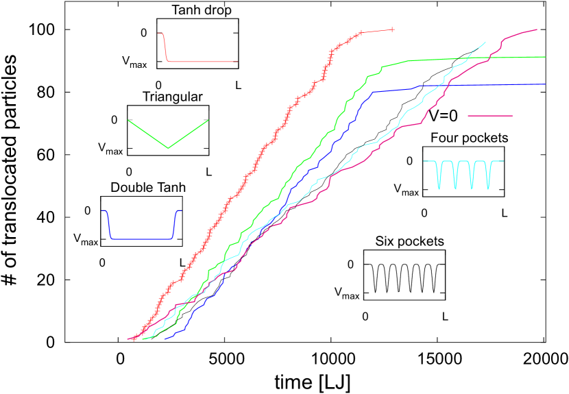
We can already make a number of observations from Fig. 6. First of all, a simple potential drop at the entrance of the channel leads to the expected acceleration and hence significantly increased the flux (red). Symmetrical potentials produce an increased flux compared to a channel with no potential ($V=0$) or different numbers of discrete binding pockets, which surprisingly produce a flux on par with the $V=0$ case. The number of translocated particles saturates at a value lower than 100, the total number of particles inserted during the simulation, because as particle insertion stops, exiting the channel becomes increasingly harder for the remaining particles since the pressure inside the channel decreases. The fact that the translocation number for a triangular potential saturates at a higher value than for the double-tanh potential supports this interpretation, since the double-tanh potential has a steeper wall at the end of the channel which will effectively block the channel.

Let us now discuss how the flux through the channel depends on the depth of the potential for the different potential functions discussed so far. We therefore define flux as the slope of a fit to the linear portion of the translocation plots in Fig. 6:

$$J=\left\langle\frac{\operatorname{d}\!N}{\operatorname{d}\!t}\right\rangle,$$ (4)

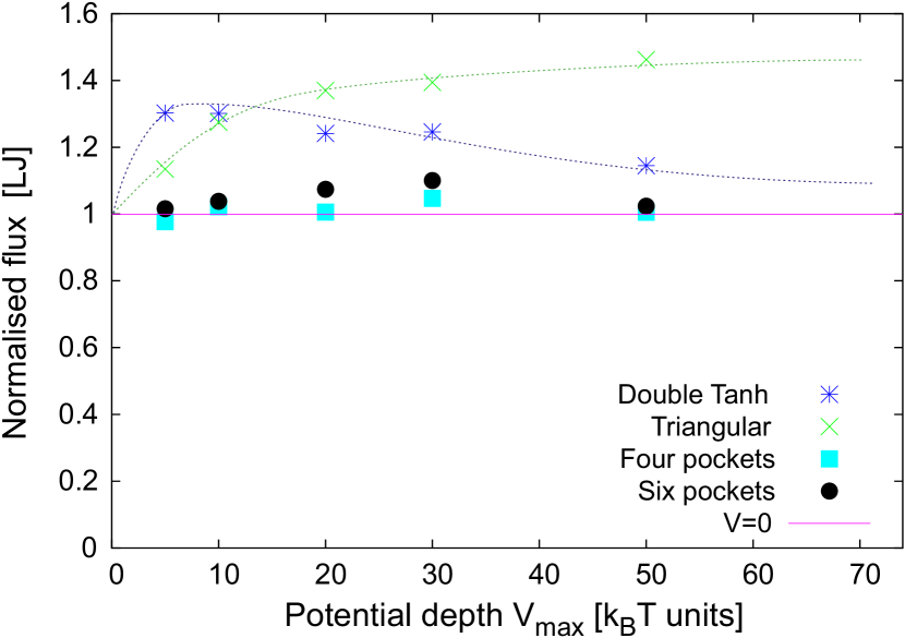
and repeat the analysis above for different potential depths. The average flux was computed from five experiments for given potential shape and depth, that simulated the translocation of 100 particles each. Simulating this number of particles stabilised the linear fits and resulted in the small relative errors that are plotted in Fig. 7 and enable us to refine some of the observations already made.

Figure 7: Normalised flux as a function of potential depth for different profiles. Fluxes are defined as the slopes of a linear fit to the cumulative plot of the number of translocated particles as a function of time (e.g. Fig. 6). Fluxes were measured from five experiments per potential shape/depth that simulated the translocation of 100 particles each and were normalised to the flux through a channel with $V=0$. The dashed lines for the three characteristic types of behaviour are to guide an eye.

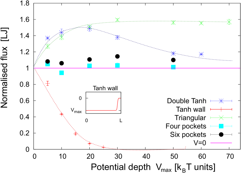
1.  Symmetric potentials increase the flux of single-file diffusion. This is surprising at first sight, since the overall work done on the particle is zero. However, the symmetry of the potentials is broken by the pressure that the newly inserted particles exert on the particles near the end of the channel at the potential wall.Lappala2013 It should be noted that this pressure emerges purely from the free diffusion inside the channel and has significant effects even at low colloid concentrations inside the channel. We are only inserting particles if there is free space at the beginning of the channel, as described above, so we are not actively pushing particles through the channel.

Furthermore, the flux through channels with symmetric potentials does not go below the flux through a free channel even for deep potentials.

2.  The triangular potential profile outperforms the double-tanh potential. This is due to the fact that in the overdamped limit, after an impulse is exerted on a particle, it quickly relaxes back to normal diffusion. Effectively, Newton’s second law does not hold anymore and a small force over a longer time, pushing the dense region forward at the entry half of the channel, is more effective than a strong force over a short period of time.

3.  The increase in flux with symmetric potentials is not due to some sort of Kramers-type barrier hoping. This is shown by the fact that the flux through a channel with a $\tanh$ step at its end (‘tanh wall’) (see inset in Fig. 7) goes to zero for $V_{\text{max}}=25$, where double-tanh and triangular potentials still outperform the $V=0$ case.

4.  Narrow binding pockets do not alter the flux significantly, even though it is clear from individual particle trajectories that particles do get trapped in the binding pockets, as we see in Fig. 5.

Figure 8: Binding potentials keep particles in the channel. The snapshots (a), (b) and (c) for different potential profiles give particle positions at the end of a simulation run, with channel and particle diameters to scale. This illustrates that sufficiently deep attractive potential will retain some particles, in regions shaded in the plots, when no additional influx from the left occurs (explaining the saturation plateau below 100 in Fig. 6).

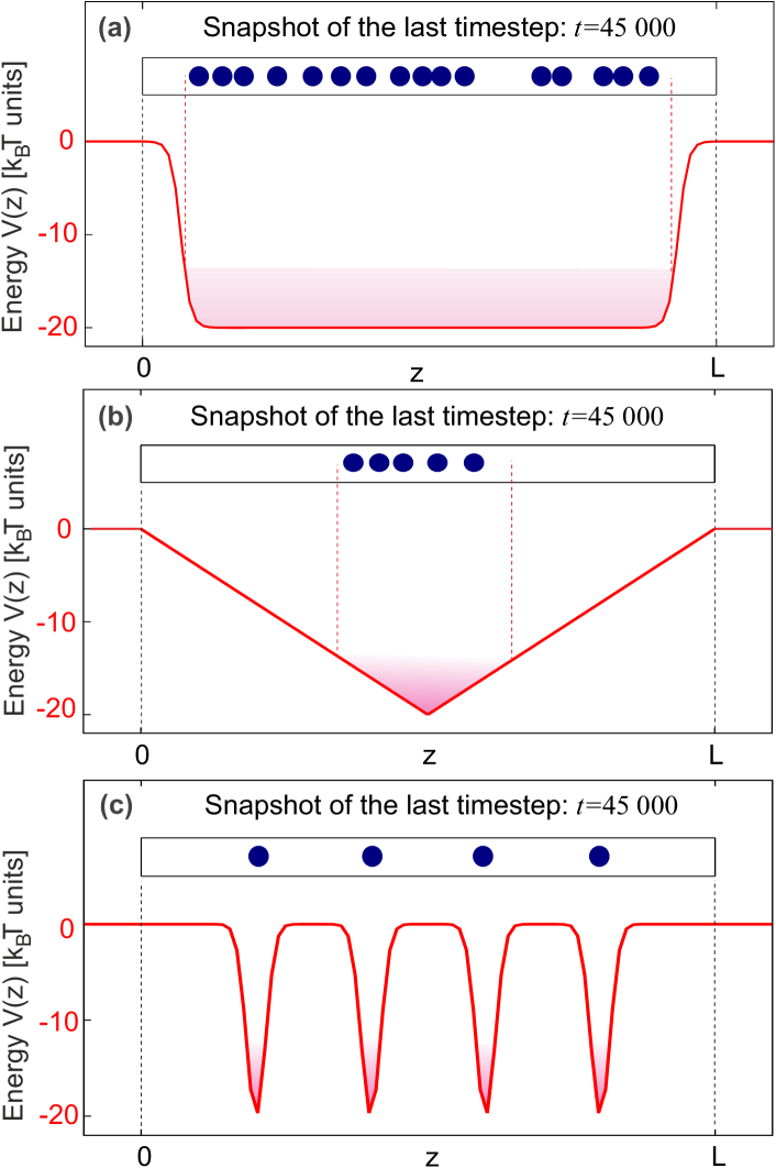
Figure 8 gives the snapshots of final simulation frames to illustrate what is an ‘equilibrium’ situation in each potential profile $V(z)$. It shows that for a sufficiently deep attractive potential well, particles are retained in such a well, while the particles facing weaker binding forces escape and diffuse out of the channel. The final number of retained particles explains why the plateaus of different curves in Fig. 6 are below 100. These snapshots also help understand why the flux increases with the depth of continuous potentials (double-tanh or triangular). The process is analogous to the enzymatic action: although the energy barrier at the end of channel is prohibitively high (as illustrated by the complete vanishing of diffusive flux for the ‘tanh-wall’ potential in Fig. 7), when particles are confined at a high density in front of such a wall – they are forced to escape, pushed by the neighbours from the left.

It is also interesting to observe that at a constant temperature of our heat bath, when these potentials become excessively deep, the channel does get blocked: this occurs at $V_{\text{max}}>50-60$ for the double-tanh potential, and has to be inferred to occur at a much greater depth for the triangular potential, see Fig. 7.

V Theoretical considerations

We would like to gain a better insight into the data shown in Fig. 7 from a theoretical perspective. Since the basic features of single-file diffusion have already been discussed extensively elsewhere,Levitt1973 ; Kollmann2003 ; Burada2009 we will focus our discussion here on the relative change in flux through a channel when we apply a potential.

It turns out that an effective way to pose this problem is to describe translocation as a reaction $A+B\rightarrow B$ where the colloidal particles $A$ are absorbed by a “trap” $B$, i.e. the channel exit, upon encounter. The problem of finding the flux through the channel becomes the problem of computing the rate $\kappa$ of this reaction in a crowded single-file environment with applied potentials. For systems with spherical symmetry in the limit of infinitely diluted reactants $A$, this is a classical problem of diffusion-controlled reaction kinetics, which was solved exactly by Smoluchowski,Smoluchowski1917 producing the rate $\kappa_{s}=4\pi D_{0}\rho_{0}$ where $\rho(r)$ is the density profile of reactants $A$ around the trap reaching the value $\rho_{0}$ at infinity.

In general, the reaction dynamics is governed by the diffusive Fokker-Planck equation:

$$\frac{\partial\rho}{\partial t}=D_{c}\nabla\cdot\left(\nabla\rho-\frac{F}{k_{B}T}\rho\right),$$ (5)

which takes the many-body effects into account through the inhomogeneous density profile $\rho(r)$ along the channel, which generates an osmotic pressure $\Pi(r)$ that acts as to spread the density profile via a force per particle $F=-1/\rho(r)\cdot\nabla\Pi(\rho)$.Zaccone2012 These two parameters are non-linearly coupled via the collective diffusion coefficient $D_{c}=D_{0}\cdot\partial\Pi/\partial\rho$, which makes an exact solution of this problem a formidable task even for numerics and makes us look for reasonable approximations.Zaccone2013

Figure 9: Binding potentials keep steady-state density highly non-linear. The snapshots (a), (b) and (c) for different potential profiles give the average density of particles in each case, in the steady-state transport regime (constant flux).

In our 1-dimensional case, we take $\rho(z)$ as the number of colloid particles per unit length along the channel at a given time (hence always $\rho<1$ for narrow channels), and we initially ignore the force due to the applied potential. With increasing $\rho$, it takes a given particle longer to reach the channel exit, but once it is in the vicinity of the exit, its chance of reaching it and escaping increases due to the added gradient of osmotic pressure. Using this model for the analysis of their simulations, Dorsaz and co-workers Dorsaz2010 showed that the reaction rate can be approximated well by the following expression:

$$\kappa\approx\kappa_{s}\frac{\beta\Pi(\rho_{0})}{\rho_{0}}\cdot\exp\left(\frac{-\beta\Pi(\rho_{\Delta})}{\rho_{\Delta}}\right)$$ (6)

where $\beta=1/k_{B}T,\ \rho_{0}$ is the density at the beginning of the channel, and $\rho_{\Delta}=\rho(\Delta)$ is the density a characteristic ‘encounter distance’ $\Delta$ from the channel end at which the density of colloid particles acquires structure due to interactions (in other words, where the ideal-gas linear relationship $\Pi=k_{B}T\rho$ stops being valid), see Fig. 9. Equation (6) has since been derived from first principles by Zaccone,Zaccone2013 who finds a prefactor of $\beta(\operatorname{d}\!\Pi/\operatorname{d}\!\rho)_{\rho_{0}}$ instead of $\beta\Pi(\rho_{0})/\rho_{0}$, but notes that that the two prefactors have the same dependence on $\rho_{0}$ which would indicate that the solution is qualitatively correct.

We write the osmotic pressure $\beta\Pi$ as a virial expansion in the density along the channel:

$$\beta\Pi=\rho+B_{2}\rho^{2}+B_{3}\rho^{3}+\mathcal{O}\left(\rho^{4}\right)$$ (7)

and compute $\rho$ from 1000 randomly selected snapshots of the simulations after the flux has equilibrated to its steady-state value. The virial coefficients $B_{2}$ and $B_{3}$ account for two- and three-body interactions between the particles in the channel which captures the essential dynamics since in the effectively 1-D system of the channel, the motion of a particle is dependent on the particle in front and the particle behind it.Lappala2013 $B_{2}$ and $B_{3}$ were computed for a Lennard-Jones $12/6$ potential with $\epsilon=1,\sigma=1$ that was used to model particle-particle interactions as described in section III. While $B_{2}=2\pi\int_{0}^{\infty}r^{2}[1-e^{-\beta V(r)}]\operatorname{d}\!r$; computation of $B_{3}$ is more involved, but values are available.Bird1950

Figure 10: Reaction rates (6) for an absorption reaction $A+B\rightarrow B$ correctly predict the flux through a channel with applied potential. The trends seen in the simulations (Fig. 7) are correctly predicted and numerical agreement is also good, although there is a systematic offset of $\sim 0.1$. Since the form of the potentials does not enter the model at any point, we conclude that all the information is encoded in the equilibrium density distribution, which we sample at only two discrete points.

A plot of the reaction rates computed from (6) is shown in Fig. 10. All values are normalised with respect to the reaction rate computed for no potential, $\kappa_{V=0}=1$. It is clear from the graph that these rates correctly predict the trends seen in the flux from the simulations (Fig. 7): there is no significant flux change with discrete pockets but a considerable increase with continuous potentials; the double tanh potential performs best at small potential depths while the triangular potential trumps at higher values of $V_{max}$. The numerical range of the relative changes is good although it is systemically low by $~{}0.1$. This is a remarkable agreement given that at no point we explicitly introduced the form of the potentials and evaluate $\rho$ only at two discrete points, i.e. the beginning of the channel and very close to its exit. This shows that all the information about many-particle effects and the channel translocation with an applied potential is encoded in the steady-state density distribution, which in turn is controlled by the two virial coefficients $B_{2}$ and $B_{3}$ (or the two values $\rho_{0}$ and $\rho_{\Delta}$ sampled near the beginning and near the end of the channel).

VI Conclusion

Our result that continuous, symmetrical potentials increase the flux significantly confirms earlier speculation that membrane channels in cells are most likely to provide a “molecular slide” Schirmer1995 by organising discrete binding sites in succession, since having them isolated one after the other would provide little to no increase in flux as shown. Furthermore, our results can offer guidance for the design of artificial channels in microfluidic applications, where improving flux is often important and clogging can be a problem Lappala2013 .

Any theoretical description of particle translocation has to account for both the applied potential and the crowding inside the channel. We have shown that it is possible to account for the relative changes in flux by considering the kinetics of the “absorption reaction” of particles exiting the channel, thus mapping the many-body problem to a two-body-interaction where crowding is modelled by the osmotic pressure inside the channel, without knowledge of the applied potential. However, this is more of an explanation a posteriori since it requires knowledge of the density profile along the channel. Further theoretical work will therefore have to focus on the development of methods to calculate these distributions not just for periodic boundary conditionsKollmann2003 , but for more realistic geometries and boundary conditions in the presence of potentials in an attempt to predict particle flux without resorting to simulations.

References

- (1) B. Alberts et al., Molecular Biology of the Cell, Garland Science, New York, 2008.
- (2) R. Shah et al., Mater. Today 11, 18 (2008).
- (3) S. Pagliara, C. Schwall, and U. F. Keyser, Adv. Mater. 25, 844 (2013).
- (4) K. Sugano et al., Nat. Rev. Drug Discov. 9, 597 (2010).
- (5) B. Hille, Ion channels of excitable membranes, Sinauer Sunderland, MA, 2001.
- (6) T. Schirmer, T. Keller, Y. Wang, and J. Rosenbusch, Science 267, 512 (1995).
- (7) J. J. Kasianowicz, T. L. Nguyen, and V. M. Stanford, Proc. Natl. Acad. Sci. 103, 11431 (2006).
- (8) C. Hilty and M. Winterhalter, Phys. Rev. Lett. 86, 5624 (2001).
- (9) M. O. Jensen, S. Park, E. Tajkhorshid, and K. Schulten, Proc. Natl. Acad. Sci. 99, 6731 (2002).
- (10) A. Kolomeisky, Phys. Rev. Lett. 98, 048105 (2007).
- (11) N. Dorsaz, C. De Michele, F. Piazza, P. De Los Rios, and G. Foffi, Phys. Rev. Lett. 105, 120601 (2010).
- (12) J. C. Chen and A. S. Kim, Adv. Colloid Interface Sci. 112, 159 (2004).
- (13) S. J. Plimpton, J. Comput. Phys. 117, 1 (1995).
- (14) G. Uhlenbeck and L. Ornstein, Phys. Rev. 36, 823 (1930).
- (15) T. Schneider and E. Stoll, Phys. Rev. B 17, 1302 (1978).
- (16) T. Al-Shemmeri, Engineering Fluid Mechnanics, Ventus Publishing ApS, 2012.
- (17) T. E. Oliphant, Comput. Sci. Eng. 9, 10 (2007).
- (18) I. Vattulainen, M. Karttunen, G. Besold, and J. M. Polson, J. Chem. Phys. 116, 3967 (2002).
- (19) The LAMMPS Team, Lammps documentation, http://lammps.sandia.gov/doc/units.html, 2014.
- (20) E. M. Nestorovich, C. Danelon, M. Winterhalter, and S. M. Bezrukov, Proc. Natl. Acad. Sci. 99, 9789 (2002).
- (21) A. Lappala, A. Zaccone, and E. M. Terentjev, Sci. Rep. 3, 3103 (2013).
- (22) D. Levitt, Phys. Rev. A 8, 3050 (1973).
- (23) M. Kollmann, Phys. Rev. Lett. 90, 180602 (2003).
- (24) P. S. Burada, P. Hänggi, F. Marchesoni, G. Schmid, and P. Talkner, Chemphyschem 10, 45 (2009).
- (25) M. Smoluchowski, Z. phys. Chem. 92, 129 (1917).
- (26) A. Zaccone and E. M. Terentjev, Phys. Rev. E 85, 061202 (2012).
- (27) A. Zaccone, J. Chem. Phys. 138, 186101 (2013).
- (28) R. B. Bird, E. L. Spotz, and J. O. Hirschfelder, J. Chem. Phys. 18, 1395 (1950).