Planar Embeddings with Small and Uniform Faces

Abstract

Motivated by finding planar embeddings that lead to drawings with favorable aesthetics, we study the problems MinMaxFace and UniformFaces of embedding a given biconnected multi-graph such that the largest face is as small as possible and such that all faces have the same size, respectively.

We prove a complexity dichotomy for MinMaxFace and show that deciding whether the maximum is at most $k$ is polynomial-time solvable for $k\leq 4$ and NP-complete for $k\geq 5$. Further, we give a 6-approximation for minimizing the maximum face in a planar embedding. For UniformFaces, we show that the problem is NP-complete for odd $k\geq 7$ and even $k\geq 10$. Moreover, we characterize the biconnected planar multi-graphs admitting 3- and 4-uniform embeddings (in a $k$-uniform embedding all faces have size $k$) and give an efficient algorithm for testing the existence of a 6-uniform embedding.

1 Introduction

While there are infinitely many ways to embed a connected planar graph into the plane without edge crossings, these embeddings can be grouped into a finite number of equivalence classes, so-called combinatorial embeddings, where two embeddings are equivalent if the clockwise order around each vertex is the same. Many algorithms for drawing planar graphs require that the input graph is provided together with a combinatorial embedding, which the algorithm preserves. Since the aesthetic properties of the drawing often depend critically on the chosen embedding, e.g. the number of bends in orthogonal drawings, it is natural to ask for a planar embedding that will lead to the best results.

In many cases the problem of optimizing some cost function over all combinatorial embeddings is NP-complete. For example, it is known that it is NP-complete to test the existence of an embedding that admits an orthogonal drawing without bends or an upward planar embedding [9]. On the other hand, there are efficient algorithms for minimizing various measures such as the radius of the dual [1, 2] and attempts to minimize the number of bends in orthogonal drawings subject to some restrictions [3, 4, 5].

Usually, choosing a planar embedding is considered as deciding the circular ordering of edges around vertices. It can, however, also be equivalently viewed as choosing the set of facial cycles, i.e., which cycles become face boundaries. In this sense it is natural to seek an embedding whose facial cycles have favorable properties. For example, Gutwenger and Mutzel [11] give algorithms for computing an embedding that maximizes the size of the outer face. The most general form of this problem is as follows. The input consists of a graph and a cost function on the cycles of the graph, and we seek a planar embedding where the sum of the costs of the facial cycles is minimum. This general version of the problem has been introduced and studied by Mutzel and Weiskircher [13]. Woeginger [14] shows that it is NP-complete even when assigning cost 0 to all cycles of size up to $k$ and cost 1 for longer cycles. Mutzel and Weiskircher [13] propose an ILP formulation for this problem based on SPQR-trees.

In this paper, we focus on two specific problems of this type, aimed at reducing the visual complexity and eliminating certain artifacts related to face sizes from drawings. Namely, large faces in the interior of a drawing may be perceived as holes and consequently interpreted as an artifact of the graph. Similarly, if the graph has faces of vastly different sizes, this may leave the impression that the drawn graph is highly irregular. However, rather than being a structural property of the graph, it is quite possible that the artifacts in the drawing rather stem from a poor embedding choice and can be avoided by choosing a more suitable planar embedding.

We thus propose two problems. First, to avoid large faces in the drawing, we seek to minimize the size of the largest face; we call this problem MinMaxFace. Second, we study the problem of recognizing those graphs that admit perfectly uniform face sizes; we call this problem UniformFaces. Both problems can be solved by the ILP approach of Mutzel and Weiskircher [13] but were not known to be NP-hard.

Our Contributions.

First, in Section 3, we study the computational complexity of MinMaxFace and its decision version $k$-MinMaxFace, which asks whether the input graph can be embedded such that the maximum face size is at most $k$. We prove a complexity dichotomy for this problem and show that $k$-MinMaxFace is polynomial-time solvable for $k\leq 4$ and NP-complete for $k\geq 5$. Our hardness result for $k\geq 5$ strengthens Woeginger’s result [14], which states that it is NP-complete to minimize the number of faces of size greater than $k$ for $k\geq 4$, whereas our reduction shows that it is in fact NP-complete to decide whether such faces can be completely avoided. Furthermore, we give an efficient 6-approximation for MinMaxFace.

Second, in Section 4, we study the problem of recognizing graphs that admit perfectly uniform face sizes (UniformFaces), which is a special case of $k$-MinMaxFace. An embedding is $k$-uniform if all faces have size $k$. We characterize the biconnected multi-graphs admitting a $k$-uniform embedding for $k=3,4$ and give an efficient recognition algorithm for $k=6$. Finally, we show that for odd $k\geq 7$ and even $k\geq 10$, it is NP-complete to decide whether a planar graph admits a $k$-uniform embedding.

2 Preliminaries

A graph $G=(V,E)$ is connected if there is a path between any two vertices. A cutvertex is a vertex whose removal disconnects the graph. A separating pair $\{u,v\}$ is a pair of vertices whose removal disconnects the graph. A connected graph is biconnected if it does not have a cutvertex and a biconnected graph is 3-connected if it does not have a separating pair. Unless specified otherwise, throughout the rest of the paper we will consider graphs without loops, but with possible multiple edges.

We consider $st$-graphs with two special pole vertices $s$ and $t$. The family of $st$-graphs can be constructed in a fashion very similar to series-parallel graphs. Namely, an edge $st$ is an $st$-graph with poles $s$ and $t$. Now let $G_{i}$ be an $st$-graph with poles $s_{i},t_{i}$ for $i=1,\dots,k$ and let $H$ be a planar graph with two designated adjacent vertices $s$ and $t$ and $k+1$ edges $st,e_{1},\dots,e_{k}$. We call $H$ the skeleton of the composition and its edges are called virtual edges; the edge $st$ is the parent edge and $s$ and $t$ are the poles of the skeleton $H$. To compose the $G_{i}$’s into an $st$-graph with poles $s$ and $t$, we remove the edge $st$ from $H$ and replace each $e_{i}$ by $G_{i}$ for $i=1,\dots,k$ by removing $e_{i}$ and identifying the poles of $G_{i}$ with the endpoints of $e_{i}$. In fact, we only allow three types of compositions: in a series composition the skeleton $H$ is a cycle of length $k+1$, in a parallel composition $H$ consists of two vertices connected by $k+1$ parallel edges, and in a rigid composition $H$ is 3-connected.

For every biconnected planar graph $G$ with an edge $st$, the graph $G-st$ is an $st$-graph with poles $s$ and $t$ [6]. Much in the same way as series-parallel graphs, the $st$-graph $G-st$ gives rise to a (de-)composition tree $\mathcal{T}$ describing how it can be obtained from single edges. The nodes of $\mathcal{T}$ corresponding to edges, series, parallel, and rigid compositions of the graph are Q-, S-, P-, and R-nodes, respectively. To obtain a composition tree for $G$, we add an additional root Q-node representing the edge $st$. We associate with each node $\mu$ the skeleton of the composition and denote it by $\operatorname{skel}(\mu)$. For a Q-node $\mu$, the skeleton consists of the two endpoints of the edge represented by $\mu$ and one real and one virtual edge between them representing the rest of the graph. For a node $\mu$ of $\mathcal{T}$, the pertinent graph $\operatorname{pert}(\mu)$ is the subgraph represented by the subtree with root $\mu$. For a virtual edge $\varepsilon$ of a skeleton $\operatorname{skel}(\mu)$, the expansion graph of $\varepsilon$ is the pertinent graph $\operatorname{pert}(\mu^{\prime})$ of the neighbor $\mu^{\prime}$ corresponding to $\varepsilon$ when considering $\mathcal{T}$ rooted at $\mu$.

The SPQR-tree of $G$ with respect to the edge $st$, originally introduced by Di Battista and Tamassia [6], is the (unique) smallest decomposition tree $\mathcal{T}$ for $G$. Using a different edge $s^{\prime}t^{\prime}$ of $G$ and a composition of $G-s^{\prime}t^{\prime}$ corresponds to rerooting $\mathcal{T}$ at the node representing $s^{\prime}t^{\prime}$. It thus makes sense to say that $\mathcal{T}$ is the SPQR-tree of $G$. The SPQR-tree of $G$ has size linear in $G$ and can be computed in linear time [10]. Planar embeddings of $G$ correspond bijectively to planar embeddings of all skeletons of $\mathcal{T}$; the choices are the orderings of the parallel edges in P-nodes and the embeddings of the R-node skeletons, which are unique up to a flip. When considering rooted SPQR-trees, we assume that the embedding of $G$ is such that the root edge is incident to the outer face, which is equivalent to the parent edge being incident to the outer face in each skeleton. We remark that in a planar embedding of $G$, the poles of any node $\mu$ of $\mathcal{T}$ are incident to the outer face of $pert(\mu)$. Hence, in the following we only consider embeddings of the pertinent graphs with their poles lying on the same face.

3 Minimizing the Maximum Face

In this section we present our results on MinMaxFace. We first strengthen the result of Woeginger [14] and show that $k$-MinMaxFace is NP-complete for $k\geq 5$ and then present efficient algorithms for $k=3,4$. In particular, the hardness result also implies that the problem MinMaxFace is NP-hard. Finally, we give an efficient $6$-approximation for MinMaxFace on biconnected graphs. Recall that we allow graphs to have multiple edges.

Theorem 3.1

$k$-MinMaxFace is NP-complete for any $k\geq 5$.

Proof

Clearly, the problem is in NP, since we can simply guess a planar embedding and verify in polynomial time that all faces have size at most $k$.

We show hardness for $k=5$ and in the end briefly sketch how to adapt the proof for $k>5$. We give a reduction from Planar $3$-Sat with the additional assumption that each variable occurs three times and each clause has size two or three. Further, we can assume that if a variable occurs three times, then it appears twice as a positive literal and once as a negative literal. This variant is NP-complete [7, Lemma 2.1].

We construct gadgets where some of the edges are in fact two parallel paths, one consisting of a single edge and one of length 2 or 3. The ordering of these paths then decides which of the faces incident to the gadget edge is incident to a path of length 1 and which is incident to a path of length 2 or 3; see Fig. 1a. Due to this use, we also call these gadgets $(1,2)$- and $(1,3)$-edges, respectively.

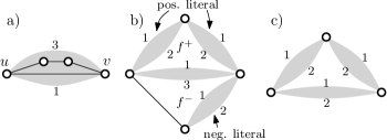
Figure 1: Illustration of the gadgets for the proof of Theorem 3.1. (a) A $(1,3)$-edge. (b) A variable gadget for a variable that occurs twice as a positive literal and once as a negative literal. Changing the flip of the $(1,3)$-edge in the middle (variable edge) forces flipping the upper two literal edges. (c) A clause gadget for a clause of size 3.

Now consider a variable $x$ whose positive literals occur $d^{+}$ times. Note that the negative literal hence occurs $3-d^{+}$ times. We represent $x$ by a variable gadget consisting of two cycles $C^{+}$ and $C^{-}$ of lengths $5-d^{+}$ and $5-(3-d^{+})=2+d^{+}$, respectively, sharing one edge. The shared edge is actually a $(1,3)$-edge, called variable edge, and in $C^{+}$ (in $C^{-}$), we replace $d^{+}$ of its edges ($3-d^{+}$ of its edges) by $(1,2)$-edges, called positive (negative) literal edges, respectively; see Fig. 1b. We denote the faces bounded solely by $C^{+}$ and $C^{-}$ by $f^{+}$ and $f^{-}$, respectively. Without loss of generality, we assume that the gadget is embedded so that $f^{+}$ and $f^{-}$ are inner faces, and we denote the outer face by $f_{0}$. The gadget represents truth values as follows. A literal edge represents the truth value true if and only if its path of length 1 is incident to the outer face. A variable edge represents value true if and only if its path of length 1 is incident to $f^{+}$. If the variable edge represents value true, then $f^{-}$ is incident to a path of length 3 of the variable edge. Hence, all negative literal edges must transmit value false. A symmetric argument shows that if the variable edge encodes value false, then all positive literal edges must transmit value false. On the other hand, given a truth value for variable $x$, choosing the flips of the variable edge and all literal edges accordingly yields an embedding where each inner face has size at most $5$.

A clause gadget for a clause of size 3 consists of a cycle of three $(1,2)$-edges that correspond bijectively to the literals occurring in it; see Fig. 1c. Similarly, a clause of size 2 consists of a cycle on four edges, two of which are $(1,2)$-edges corresponding to the literals. The encoding is such that a literal edge has its path of length 2 incident to the inner face of the clause gadget if and only if such a literal has value false. Clearly, the inner face has size at most 5 if and only if at most two literals transmit value false, otherwise the size is 6. Thus, the inner face of the clause gadget has size at most 5 if and only if at least one the literals transmit value true.

We now construct a graph $G_{\varphi}$ as follows. We create for each variable a corresponding variable gadget and for each clause a corresponding clause gadget. We then identify literal edges of variables and clauses that correspond to the same literal. By adhering to the planar embedding of the variable–clause graph of $\varphi$, the resulting graph $G_{\varphi}$ is planar and can be embedded such that all inner faces of the gadgets are faces of the graph. Denote this plane graph by $H_{\varphi}$. To obtain $G_{\varphi}$, we arbitrarily triangulate all faces of $H_{\varphi}$ that are not internal faces of a gadget. Then, the only embedding choices of $G_{\varphi}$ are the flips of the $(1,2)$- and $(1,3)$-edges. We claim that $G_{\varphi}$ admits an embedding where every face has size at most 5 if and only if $\varphi$ is satisfiable.

If $G$ is satisfiable, pick a satisfying truth assignment. We flip each variable edge and each literal edge to encode its truth value in the assignment. As argued above, every inner face of a variable now has size at most 5, and, since each clause contains at least one satisfied literal, also the inner faces of the clause gadgets have size at most 5. Conversely, given a planar embedding of $G_{\varphi}$ where each face has size at most 5, we construct a satisfying truth assignment for $\varphi$ by assigning a variable the truth value encoded by the variable edge in the corresponding gadget. Due to the above properties, it follows that all edges corresponding to a negative literal must contribute a path of length 2 to each clause gadget containing such a literal. However, each inner face of a clause gadget has only size 5, and hence at least one of the literal edges must contribute a path of only length 1, i.e., the clause contains a satisfied literal. Since the construction of $G_{\varphi}$ can clearly be done in polynomial time, this finishes the proof for $k=5$.

For $k>5$, it suffices to lengthen all cycles of the construction by $k-5$ edges. All arguments naturally carry over.

3.1 Polynomial-Time Algorithm for Small Faces

Next, we show that $k$-MinMaxFace is polynomial-time solvable for $k=3,4$. Note that, if the input graph is simple, the problem for $k=3$ is solvable if and only if the input graph is maximal planar. A bit more work is necessary if we allow parallel edges.

Let $G$ be a biconnected planar graph. We devise a dynamic program on the SPQR-tree $\mathcal{T}$ of $G$. Let $\mathcal{T}$ be rooted at an arbitrary Q-node and let $\mu$ be a node of $\mathcal{T}$. We call the clockwise and counterclockwise paths connecting the poles of $\mu$ along the outer face the boundary paths of $\operatorname{pert}(\mu)$. We say that an embedding of $\operatorname{pert}(\mu)$ has type $(a,b)$ if and only if all its inner faces have size at most $k$ and its boundary paths have length $a$ and $b$, respectively. Such an embedding is also called an $(a,b)$-embedding. We assume that $a\leq b$.

Clearly, each of the two boundary paths of $\operatorname{pert}(\mu)$ in an embedding $\mathcal{E}_{\mu}$ of type $(a,b)$ will be a proper subpath of the boundary of a face in any embedding of $G$ where the embedding of $\operatorname{pert}(\mu)$ is $\mathcal{E}_{\mu}$. Hence, when seeking an embedding where all faces have size at most $k$, we are only interested in the embedding $\mathcal{E}_{\mu}$ if $1\leq a\leq b\leq k-1$. We define a partial order on the embedding types by $(a^{\prime},b^{\prime})\preceq(a,b)$ if and only if $a^{\prime}\leq a$ and $b^{\prime}\leq b$. Replacing an $(a,b)$-embedding $\mathcal{E}_{\mu}$ of $\operatorname{pert}(\mu)$ by (a reflection of) an $(a^{\prime},b^{\prime})$-embedding $\mathcal{E}_{\mu}^{\prime}$ with $(a^{\prime},b^{\prime})\preceq(a,b)$ does not create faces of size more than $k$; all inner faces of $\mathcal{E}_{\mu}^{\prime}$ have size at most $k$ by assumption, and the only other faces affected are the two faces incident to the two boundary paths of $\mathcal{E}_{\mu}^{\prime}$, whose length does not increase. We thus seek to compute for each node $\mu$ the minimal pairs $(a,b)$ for which it admits an $(a,b)$-embedding. We remark that $\operatorname{pert}(\mu)$ can admit an embedding of type $(1,b)$ for any value of $b$ only if $\mu$ is either a P-node or a Q-node.

We now present the algorithm for $k=3$, which works even if we allow parallel edges.

Theorem 3.2

3-MinMaxFace can be solved in linear time for biconnected graphs.

Proof

Clearly, the only interesting types of embeddings are $(1,1),(1,2)$ and $(2,2)$ and $\preceq$ defines a total ordering on them. We thus seek to determine for each pertinent graph bottom-up in the SPQR-tree the smallest type (with respect to $\preceq$) of a valid planar embedding. For Q-nodes this is $(1,1)$. Now consider an R-node or S-node $\mu$. By the above remark its only possible type of embedding can be $(2,2)$. Since every face is bounded by at least three edges, it is not hard to see that $\operatorname{pert}(\mu)$ admits a $(2,2)$-embedding if and only if every face of $\operatorname{skel}(\mu)$ has size 3 and all children admit $(1,1)$-embeddings.

For a P-node, we observe that none of its children can have a $(1,2)$-embedding, as no two P-node can be adjacent. Thus, all children admit either a $(1,1)$-embedding, then they are Q-nodes, or they admit a $(2,2)$-embedding. We denote the virtual edges in $\operatorname{skel}(\mu)$ by $(1,1)$-edges and $(2,2)$-edges, respectively, according to the type of embedding the corresponding graph admits. To obtain an embedding where all faces have size at most 3, we have to choose the embedding of $\operatorname{skel}(\mu)$ in such a way that every $(2,2)$-edge is adjacent to either two $(1,1)$-edges or to a $(1,1)$-edge and the parent edge. Let $a$ and $b$ denote the number of $(1,1)$-edges and $(2,2)$-edges in $\operatorname{skel}(\mu)$, respectively. Clearly, an ordering satisfying these requirements exists if and only if $a\geq b-1$; otherwise we necessarily have two adjacent $(2,2)$-edges. To find a good sequence, we proceed as follows. If $a=b-1$, the sequence must alernatingly consist of $(2,2)$-edges and $(1,1)$-edges, starting with a $(1,1)$-edge. The type of the resulting embedding is $(2,2)$ and one cannot do better. If $a=b$, we do the same, but the type of the resulting embedding is $(1,2)$; again one cannot do better. Finally, if $a\geq b+1$, we again do the same, and finally append the remaining $(1,1)$-edges. Then the resulting embedding has type $(1,1)$.

Clearly, we can process each node $\mu$ in time proportional to the size of its skeleton. The graph admits an embedding if and only if the pertinent graph of the child of the root admits some valid embedding.

We now deal with the case $k=4$, which is similar but more complicated. The relevant types are $(1,1),(1,2),(1,3),(2,2),(2,3)$, and $(3,3)$. We note that precisely the two elements $(2,2)$ and $(1,3)$ are incomparable with respect to $\preceq$. Thus, it seems that, rather than computing only the single smallest type for which each pertinent graph admits an embedding, we are now forced to find all minimum pairs for which the pertinent graph admits a corresponding embedding. However, by the above observation, if a pertinent graph $\operatorname{pert}(\mu)$ admits a $(1,3)$-embedding, then $\mu$ must be a P-node. However, if the parent of $\mu$ is an S-node or an R-node, then using a $(1,3)$-embedding results in a face of size at least 5. Thus, such an embedding can only be used if the parent is the root Q-node. If there is the choice of a $(2,2)$-embedding in this case, it can of course also be used at the root. Therefore, we can mostly ignore the $(1,3)$-case and consider the linearly ordered embedding types $(1,1),(1,2),(2,2),(2,3)$ and $(3,3)$. The type $(1,3)$ is only relevant for P-nodes whose pertinent graph admits an embedding of type $(1,3)$ embedding but no embedding of type $(2,2)$.

Theorem 3.3

4-MinMaxFace can be solved in $O(n^{1.5})$ time for biconnected graphs.

Proof

We process the SPQR-tree of the input graph in a bottom-up fashion. The pertinent graphs of Q-nodes admit embeddings of type $(1,1)$.

Now consider an S- or an R-node $\mu$. All faces of $\operatorname{skel}(\mu)$ must have size at most 4. Moreover, since all faces have length at least 3, a valid embedding of $\operatorname{pert}(\mu)$ does not exist if some child only allows embeddings of type $(1,3)$, $(2,3)$ or $(3,3)$. Thus, the only freedom is to choose the flips of the pertinent graphs admitting only $(1,2)$-embeddings. A face can receive only a single path of length 2 from one of its incident edges, and this is possible only if the face is a triangle and none of its incident edges is a $(2,2)$-edge. We thus seek a matching between the $(1,2)$-edges and their incident faces that can receive a path of length 2. Depending on the size of the faces incident to the parent edge and whether they need to receive a path of length 2 in order to find a valid embedding, the type is either $(2,2)$ (if both faces are triangles and they do not need to receive a path of length 2), $(2,3)$ (if one is a triangle that does not need to receive a path of length 2) or $(3,3)$ (remaining cases).

Now consider a P-node. Each child must have an embedding of type $(1,1)$, $(2,2)$, $(2,3)$ or $(3,3)$. Again, we denote the edges whose corresponding pertinent graph admits an embedding of type $(a,b)$ as $(a,b)$-edges.

First observe that removing in any embedding all $(2,2)$-edges except for one and placing them next to the single $(2,2)$-edge we did not remove results in a valid embedding whose boundary paths do not increase. Thus, we can assume without loss of generality that there is at most one $(2,2)$-edge. Moreover, if there is a $(2,3)$-edge, we can actually move the $(2,2)$-edge next to it without increasing the size of any face. Thus, if there are any $(2,3)$-edges we can even assume that there is no $(2,2)$-edge.

Let us first assume that there is no $(2,3)$-edge. We then have to choose the embedding such that $(1,1)$-edges alternate with $(3,3)$-edges and the single $(2,2)$-edge. We append any excess of $(1,1)$-edges at the end. Let $a$ denote the number of $(1,1)$-edges and let $b$ denote the total number of $(2,2)$ and $(3,3)$-edges. A valid embedding exists only if $a\geq b-1$. In this case a suitable sequence always exists. If possible, we start and end with a $(1,1)$-edge, resulting in a $(1,1)$-embedding. If this is not the case, we try to start with a $(1,1)$ and put the $(2,2)$ in the end if it exists. Then we obtain a $(1,2)$-embedding if there is a $(2,2)$-edge and a $(1,3)$-embedding otherwise. If this is also not possible since $a=b-1$, we start with the $(2,2)$-edge if it exists. This results in either a $(2,3)$ or a $(3,3)$-embedding.

The bottleneck concerning the running time is finding the matching for treating the R-node, which can be solved in $O(n^{1.5})$ time [8].

3.2 Approximation Algorithm

In this section, we present a constant-factor approximation algorithm for the problem of minimizing the largest face in an embedding of a biconnected graph $G=(V,E)$. We again solve the problem by dynamic programming on the SPQR-tree of $G$.

Let $G$ be a biconnected planar graph, and let $\mathcal{T}$ be its SPQR-tree, rooted at an arbitrary Q-node. Let $\mu$ be a node of $\mathcal{T}$. We shall consider the embeddings of $\operatorname{pert}(\mu)$ where the two poles are embedded on the outer face. We also include the parent edge in the embedding, by drawing it in the outer face. In such an embedding of $\operatorname{skel}(\mu)$, the two faces incident to the parent edge are called the outer faces, while the remaining faces are inner faces.

Recall that an $(a,b)$-embedding of $\operatorname{pert}(\mu)$ is an embedding whose boundary paths have lengths $a$ and $b$, where we always assume that $a\leq b$. We say that an $(a,b)$-embedding of $\operatorname{pert}(\mu)$ is out-minimal if for any $(a^{\prime},b^{\prime})$-embedding of $\operatorname{pert}(\mu)$, we have $a\leq a^{\prime}$ and $b\leq b^{\prime}$. Note that an out-minimal embedding need not exist; e.g., $\operatorname{pert}(\mu)$ may admit a $(2,4)$-embedding and a $(3,3)$-embedding, but no $(a,b)$-embedding with $a\leq 2$ and $b\leq 3$. We will later show, however, that such a situation can only occur when $\mu$ is an S-node.

Let $\textsc{Opt}(G)$ denote the smallest integer $k$ such that $G$ has an embedding whose every face has size at most $k$. For a node $\mu$ of $\mathcal{T}$, we say that an embedding of $\operatorname{pert}(\mu)$ is $c$-approximate, if each inner face of the embedding has size at most $c\cdot\textsc{Opt}(G)$.

Call an embedding of $\operatorname{pert}(\mu)$ neat if it is out-minimal and 6-approximate. The main result of this section is the next proposition.

Proposition 1

Let $G$ be a biconnected planar graph with SPQR tree $\mathcal{T}$, rooted at an arbitrary $Q$-node. Then the pertinent graph of every Q-node, P-node or R-node of $\mathcal{T}$ has a neat embedding, and this embedding may be computed in polynomial time.

Since the pertinent graph of the root of $\mathcal{T}$ is the whole graph $G$, the proposition implies a polynomial 6-approximation algorithm for minimization of largest face.

Our proof of Proposition 1 is constructive. Fix a node $\mu$ of $\mathcal{T}$ which is not an S-node. We now describe an algorithm that computes a neat embedding of $\operatorname{pert}(\mu)$, assuming that neat embeddings are available for the pertinent graphs of all the descendant nodes of $\mu$ that are not $S$-nodes. We distinguish cases based on the type of the node $\mu$.

Non-root Q-nodes.

As a base case, suppose that $\mu$ is a non-root Q-node of $\mathcal{T}$. Then $\operatorname{pert}(\mu)$ is a single edge, and its unique embedding is clearly neat.

P-nodes.

Next, suppose that $\mu$ is a P-node with $k$ child nodes $\mu_{1},\dotsc,\mu_{k}$, represented by $k$ skeleton edges $e_{1},\dotsc,e_{k}$. Let $G_{i}$ be the expansion graph of $e_{i}$. We construct the expanded skeleton $\operatorname{skel}^{*}(\mu)$ as follows: if for some $i$ the child node $\mu_{i}$ is an S-node whose skeleton is a path of length $m$, replace the edge $e_{i}$ by a path of length $m$, whose edges correspond in a natural way to the edges of $\operatorname{skel}(\mu_{i})$.

Every edge $e^{\prime}$ of the expanded skeleton corresponds to a node $\mu^{\prime}$ of $\mathcal{T}$ which is a child or a grand-child of $\mu$. Moreover, $\mu^{\prime}$ is not an S-node, and we may thus assume that we have already computed a neat embedding for $\operatorname{pert}(\mu^{\prime})$. Note that $\operatorname{pert}(\mu^{\prime})$ is the expansion graph of $e^{\prime}$.

For each $i\in\{1,\dotsc,k\}$ define $\ell_{i}$ to be the smallest value such that $G_{i}$ has an embedding with boundary path of length $\ell_{i}$. We compute $\ell_{i}$ as follows: if $\mu_{i}$ is not and S-node, then we already know a neat $(a_{i},b_{i})$-embedding of $G_{i}$, and we may put $\ell_{i}=a_{i}$. If, on the other hand, $\mu_{i}$ is an S-node, then let $m$ be the number of edges in the path $\operatorname{skel}(\mu_{i})$, and let $G_{i}^{1},G_{i}^{2},\dotsc,G_{i}^{m}$ be the expansion graphs of the edges of the path. For each $G_{i}^{j}$, we have already computed a neat $(a_{j},b_{j})$-embedding, so we may now put $\ell_{i}=\sum_{j=1}^{m}a_{j}$. Clearly, this value of $\ell_{i}$ corresponds to the definition given above.

We now fix two distinct indices $\alpha,\beta\in\{1,\dotsc,k\}$, so that the values $\ell_{\alpha}$ and $\ell_{\beta}$ are as small as possible; formally, $\ell_{\alpha}=\min\{\ell_{i};\;i=1,\dotsc,k\}$ and $\ell_{\beta}=\min\{\ell_{i};\;i=1,\dotsc,k\text{ and }i\neq\alpha\}$.

Let us fix an embedding of $\operatorname{skel}(\mu)$ in which $e_{\alpha}$ and $e_{\beta}$ are adjacent to the outer faces. We extend this embedding of $\operatorname{skel}(\mu)$ into an embedding of $\operatorname{pert}(\mu)$ by replacing each edge of $\operatorname{skel}^{*}(\mu)$ by a neat embedding of its expansion graph, in such a way that the two boundary paths have lengths $\ell_{\alpha}$ and $\ell_{\beta}$. Let $\mathcal{E}$ be the resulting $(\ell_{\alpha},\ell_{\beta})$-embedding of $\operatorname{pert}(\mu)$.

We now show that $\mathcal{E}$ is neat. From the definitions of $\ell_{\alpha}$ and $\ell_{\beta}$, we easily see that $\mathcal{E}$ is out-minimal. It remains to show that it is 6-approximate. Let $f$ be any inner face of $\mathcal{E}$. If $f$ is an inner face of the expansion graph $G_{i}$ of some $e_{i}$, then $f$ is an inner face of some previously constructed neat embedding, hence $|f|\leq 6\cdot\textsc{Opt}(G)$.

Suppose then that $f$ is not the inner face of any $G_{i}$. Then the boundary of $f$ intersects two distinct expansion graphs $G_{i}$ and $G_{j}$. Hence the boundary of $f$ is the union of two paths $P_{i}$ and $P_{j}$, with $P_{i}\subseteq G_{i}$ and $P_{j}\subseteq G_{j}$. Let $d_{i}$ and $d_{j}$ be the lengths of $P_{i}$ and $P_{j}$, respectively, and assume that $d_{i}\leq d_{j}$. It follows that $|f|=d_{i}+d_{j}\leq 2d_{j}$. We claim that every embedding of $G$ has a face of size at least $d_{j}/2$. If $\mu_{j}$ is not an S-node, this follows from the fact that $P_{j}$ is a boundary path in an out-minimal embedding of $G_{j}$, hence any other embedding of $G_{j}$ must have a boundary path of length at least $d_{j}$. If, on the other hand, $\mu_{j}$ is an S-node, then in every embedding of $G_{j}$, the two boundary paths have total length at least $d_{j}$, so every embedding of $G_{j}$ has a boundary path of length at least $d_{j}/2$ and thus $G$ has a face of size at least $d_{j}/2$. We conclude that $|f|\leq 2d_{j}\leq 4\cdot\textsc{Opt}(G)$, showing that $\mathcal{E}$ is indeed neat.

R-nodes.

Suppose now that $\mu$ is an R-node. As with P-nodes, we define the expanded skeleton $\operatorname{skel}*(\mu)$ by replacing each edge of $\operatorname{skel}(\mu)$ corresponding to an S-node by a path of appropriate length. The graph $\operatorname{skel}*(\mu)$ together with the parent edge forms a subdivision of a 3-connected graph. In particular, its embedding is determined uniquely up to a flip and a choice of outer face. Fix an embedding of $\operatorname{skel}^{*}(\mu)$ and the parent edge, so that the parent edge is on the outer face. Let $f_{1}$ and $f_{2}$ be the two faces incident to the parent edge of $\mu$.

Let $e$ be an edge of $\operatorname{skel}^{*}(\mu)$, let $G_{e}$ be its expansion graph, and let $\mathcal{E}_{e}$ be a neat $(a,b)$-embedding of $G_{e}$, for some $a\leq b$. The boundary path of $\mathcal{E}_{e}$ of length $a$ will be called the short side of $\mathcal{E}_{e}$, while the boundary path of length $b$ will be the long side. If $a=b$, we choose the long side and short side arbitrarily.

Our goal is to extend the embedding of $\operatorname{skel}^{*}(\mu)$ into an embedding of $\operatorname{pert}(\mu)$ by replacing each edge $e$ of $\operatorname{skel}^{*}(\mu)$ with a copy of $\mathcal{E}_{e}$. In doing so, we have to choose which of the two faces incident to $e$ will be adjacent to the short side of $\mathcal{E}_{e}$.

First of all, if $e$ is an edge of $\operatorname{skel}^{*}(\mu)$ incident to one of the outer faces $f_{1}$ or $f_{2}$, we embed $\mathcal{E}_{e}$ in such a way that its short side is adjacent to the outer face. Since $f_{1}$ and $f_{2}$ do not share an edge in $\operatorname{skel}^{*}(\mu)$, such an embedding is always possible, and guarantees that the resulting embedding of $\operatorname{pert}(\mu)$ will be out-minimal.

It remains to determine the orientation of $\mathcal{E}_{e}$ for the edges $e$ that are not incident to the outer faces, in such a way that the largest face of the resulting embedding will be as small as possible. Rather than solving this task optimally, we formulate a linear programming relaxation, and then apply a rounding step which will guarantee a constant factor approximation.

Intuitively, the linear program works as follows: given an edge $e$ incident to a pair of faces $f$ and $g$, and a corresponding graph $G_{e}$ with a short side of length $a$ and a long side of length $b$, rather than assigning the short side to one face and the long side to the other, we assign to each of the two faces a fractional value in the interval $[a,b]$, so that the two values assigned by $e$ to $f$ and $g$ have sum $a+b$, and the maximum total amount assigned to a single face of $\operatorname{skel}^{*}(\mu)$ from its incident edges is as small as possible.

More precisely, we consider the linear program with the set of variables

$$\{M\}\cup\{x_{e,f};\;e\text{ is an edge adjacent to face }f\},$$

where the goal is to minimize $M$ subject to the following constraints:

• For every edge $e$ adjacent to a pair of faces $f$ and $g$, we have the constraints $x_{e,f}+x_{e,g}=a+b$, $a\leq x_{e,f}\leq b$ and $a\leq x_{e,g}\leq b$, where $a\leq b$ are the lengths of the two boundary paths of $\mathcal{E}_{e}$.

• Moreover, if an edge $e$ is adjacent to an outer face $f\in\{f_{1},f_{2}\}$ as well as an inner face $g$, then we set $x_{e,f}=a$ and $x_{e,g}=b$, with $a$ and $b$ as above.

• For every inner face $f$ of $\operatorname{skel}^{*}(\mu)$, we have the constraint $\sum_{e}x_{e,f}\leq M$, where the sum is over all edges incident to $f$.

Given an optimal solution of the above linear program, we determine the embedding of $\operatorname{pert}(\mu)$ as follows: for an edge $e$ of $\operatorname{skel}^{*}(\mu)$ incident to two inner faces $f$ and $g$, if $x_{e,f}\leq x_{e,g}$, embed $\mathcal{E}_{e}$ with its short side incident to $f$ and long side incident to $g$. Let $\mathcal{E}_{\mu}$ be the resulting embedding.

We claim that $\mathcal{E}_{\mu}$ is neat. We have already seen that $\mathcal{E}_{\mu}$ is out-minimal, so it remains to show that every inner face of $\mathcal{E}_{\mu}$ has size at most $6\cdot\textsc{Opt}(G)$. Let us say that an inner face of $\mathcal{E}_{\mu}$ is deep if it is also an inner face of some $\mathcal{E}_{e}$, and it is shallow if it corresponds to a face of $\operatorname{skel}^{*}(\mu)$. Note that the deep faces have size at most $6\cdot\textsc{Opt}(G)$, since all the $\mathcal{E}_{e}$ are neat embeddings, so we only need to estimate the size of the shallow faces.

Let $\textsc{Opt}_{out}$ denote the minimum $k$ such that $\operatorname{pert}(\mu)$ has an out-minimal embedding whose every shallow face has size at most $k$. We claim that $\textsc{Opt}_{out}\leq 3\cdot\textsc{Opt}(G)$. To see this, consider an embedding of $\operatorname{pert}(\mu)$ in which each face has size at most $\textsc{Opt}(G)$. In this embedding, replace each subembedding of $G_{e}$ by a copy of $\mathcal{E}_{e}$, without increasing the size of any shallow face. This can be done, because each $\mathcal{E}_{e}$ is out-minimal. Call the resulting embedding $\mathcal{E}^{\prime}$. Next, for every edge $e$ of $\operatorname{skel}^{*}(\mu)$ adjacent to $f_{1}$ or $f_{2}$, flip $\mathcal{E}_{e}$ so that its short side is incident to $f_{1}$ or $f_{2}$. Let $\mathcal{E}^{\prime\prime}$ be the resulting embedding of $\operatorname{pert}(\mu)$. Clearly, $\mathcal{E}^{\prime\prime}$ is out-minimal.

In $\mathcal{E}^{\prime\prime}$, some inner shallow face $f$ adjacent to $f_{1}$ or $f_{2}$ may have larger size than the corresponding face of $\mathcal{E}^{\prime}$; however, for such an $f$, its size in $\mathcal{E}^{\prime\prime}$ is at most equal to the sum of the sizes of $f$, $f_{1}$ and $f_{2}$ in $\mathcal{E}^{\prime}$. In particular, each inner shallow face has size at most $3\cdot\textsc{Opt}(G)$ in $\mathcal{E}^{\prime\prime}$, and hence $\textsc{Opt}_{out}\leq 3\cdot\textsc{Opt}(G)$, as claimed.

We will now show that each shallow face of $\mathcal{E}_{\mu}$ has size at most $2\cdot\textsc{Opt}_{out}$. Let $M$ be the value of optimum solution to the linear program defined above. Clearly, $M\leq\textsc{Opt}_{out}$, since from an out-minimal embedding with shallow faces of size at most $\textsc{Opt}_{out}$, we may directly construct a feasible solution of the linear program with value $\textsc{Opt}_{out}$. Let $f$ be a shallow face of $\mathcal{E}_{\mu}$. Let $e$ be an edge of $\operatorname{skel}^{*}(\mu)$ incident to $f$, and let $g$ be the other face incident to $e$. Let $a$ and $b$ be the lengths of the short side and long side of $\mathcal{E}_{e}$, respectively. If $x_{e,f}\leq x_{e,g}$, then $\mathcal{E}_{e}$ contributes to the boundary of $f$ by its short side, which has length $a$. Otherwise, $f$ has the long side of $\mathcal{E}_{e}$ on its boundary, but that may only happen when $x_{e,f}\geq x_{e,g}$, and hence $b\leq a+b=x_{e,f}+x_{e,g}\leq 2x_{e,f}$. From this, we see that $f$ has size at most $\sum_{e}2x_{e,f}\leq 2M$, with the previous sum ranging over all edges of $\operatorname{skel}^{*}(\mu)$ incident to $f$.

Thus, for every shallow face $f$ of $\mathcal{E}_{\mu}$, we have $|f|\leq 2M\leq 2\cdot\textsc{Opt}_{out}\leq 6\cdot\textsc{Opt}(G)$, showing that $\mathcal{E}_{\mu}$ is neat.

The root Q-node.

Finally, suppose that $\mu$ is the root of the SPQR-tree $\mathcal{T}$. That means that $\mu$ is a Q-node, and its skeleton is formed by two parallel edges $e_{1}$ and $e_{2}$, where the expansion graph of $e_{1}$ is a single edge and the expansion graph $G_{2}$ of $e_{2}$ is the pertinent graph of the unique child node $\mu^{\prime}$ of $\mu$. If $\mu^{\prime}$ is not an S-node, we already have a neat $(a,b)$-embedding $\mathcal{E}_{2}$ of $G_{2}$, and by inserting the edge $e_{1}$ to this embedding in such a way that the outer face has size $a+1$, we clearly obtain a neat embedding of $G$. If $\mu^{\prime}$ is an S-node, then $G_{2}$ is a chain of biconnected graphs $G_{2}^{1},G_{2}^{2},\dotsc,G_{2}^{k}$, and for each $G_{2}^{i}$ we have a neat $(a_{i},b_{i})$-embedding. Combining these embedding in an obvious way, and adding the edge $e_{1}$, we get an embedding of $G$ whose outer face has size $1+a_{1}+a_{2}+\dotsb+a_{k}$, and whose unique inner shallow face has size $1+b_{1}+b_{2}+\dotsb+b_{k}$. Since in each embedding of $G$, the two faces incident to $e_{1}$ have total size at least $2+a_{1}+\dotsb+a_{k}+b_{1}+\dotsb+b_{k}$, we conclude that our embedding of $G$ is neat.

This completes the proof of Proposition 1, and yields a 6-approximation algorithm for the minimization of largest face in biconnected graphs.

Theorem 3.4

A $6$-approximation for MinMaxFace in biconnected graphs can be computed in polynomial time.

4 Perfectly Uniform Face Sizes

In this section we study the problem of deciding whether a biconnected planar graph admits a $k$-uniform embedding. Note that, due to Euler’s formula, a connected planar graph with $n$ vertices and $m$ edges has $f=m-n+2$ faces. In order to admit an embedding where every face has size $k$, it is necessary that $2m=fk$. Hence there is at most one value of $k$ for which the graph may admit a $k$-uniform embedding.

In the following, we characterize the graphs admitting 3-uniform and 4-uniform embeddings, and we give an efficient algorithm for testing whether a graph admits a 6-uniform embedding. Finally, we show that testing whether a graph admits a $k$-uniform embedding is NP-complete for odd $k\geq 7$ and even $k\geq 10$. We leave open the cases $k=5$ and $k=8$.

Our characterizations and our testing algorithm use the recursive structure of the SPQR-tree. To this end, it is necessary to consider embeddings of pertinent graphs, where we only require that the interior faces have size $k$, whereas the outer face may have different size, although it must not be too large. We call such an embedding almost $k$-uniform. The following lemma states that the size of the outer face in such an embedding depends only on the number of vertices and edges in the pertinent graph.

Lemma 1

Let $G$ be a graph with $n$ vertices and $m$ edges with an almost $k$-uniform embedding. Then the outer face has length $\ell=k(n-m-1)+2m$.

Proof

Let $f$ denote the number of faces of $G$ in a planar embedding, which us uniquely determined by Euler’s formula $n-m+f=2$. By double counting, we find that $(f-1)\cdot k+\ell=2m$. Euler’s formula implies that $f=2+m-n$, and plugging this into the second formula, we obtain that $(1+m-n)\cdot k+\ell=2m$ or, equivalently, $\ell=k(n-m-1)+2m$.

Thus, for small values of $k$, where the two boundary paths of the pertinent graph may have only few different lengths, the type of an almost $k$-uniform embedding is essentially fixed.

4.1 Characterization for $k=3,4$

For 3-uniform embeddings first observe that every facial cycle must be a triangle. If the input graph is simple, then this implies that it must be a triangulation. Then the graph is 3-connected and the planar embedding is uniquely determined. We characterize the multi-graphs that have such an embedding.

Theorem 4.1

A biconnected planar graph $G$ admits $3$-uniform embedding if and only if its SPQR-tree satisfies all of the following conditions.

1. S- and R-nodes are only adjacent to Q- and P-nodes.

2. Every R-node skeleton is a planar triangulation.

3. Every S-node skeleton has size 3.

4. Every P-node with $k$ neighbors has $k$ even and precisely $k/2$ of the neighbors are Q-nodes.

Proof

It is not hard to see that all conditions are necessary. We prove sufficiency. To this end, we choose the embeddings of the R-node skeletons arbitrarily, and we embed the P-node skeletons such that virtual edges corresponding to Q-node and non-Q-node neighbors alternate. We claim that in the resulting planar embedding of $G$ all faces have size 3.

To this end, root the SPQR-tree $\mathcal{T}$ of $G$ at an arbitrary edge $e$ and consider the embedding $e$ incident to the outer face.

Claim

1. If $\mu$ is a Q-node or a P-node whose parent is not a Q-node, then it has an almost 3-uniform embedding of type $(1,1)$.

2. If $\mu$ is an S-node, an R-node, or a P-node whose parent is a Q-node, then it has an almost 3-uniform embedding of type $(2,2)$.

We prove this by induction on the height of the node in the SPQR-tree. Clearly, the statement holds for Q-nodes. Now consider an internal node $\mu$ and assume that the claim holds for all children.

If $\mu$ is an S-node, then the clockwise (counterclockwise) path of $\operatorname{pert}(\mu)$ between the poles along the outer face is the concatenation of the clockwise path (counterclockwise) paths of the pertinent graphs of its children. By property (iii) there are only two children and by property (i) they are either Q- or P-nodes. By the inductive hypothesis, their embeddings are almost 3-uniform and have type $(1,1)$, and hence the type of the embedding of $\operatorname{pert}(\mu)$ is $(2,2)$.

If $\mu$ is an R-node, then its clockwise (counterclockwise) path between the poles is the concatenation of the clockwise (counterclockwise) paths of the pertinent graphs corresponding to the edges on the clockwise (counterclockwise) path between the poles. By property (ii) each of these paths has length 2 in $\operatorname{skel}(\mu)$ and the children are either Q- or P-nodes. Thus, by the inductive hypothesis, their embeddings have type $(1,1)$.

If $\mu$ is a P-node whose parent is not a Q-node, then, by our choice of the planar embedding, the two outer paths in $\operatorname{skel}(\mu)$ are edges corresponding to Q-nodes, and the claim follows from the inductive hypothesis. If the parent of $\mu$ is a Q-node, then, again by the embedding choice, the two edges outer paths in $\operatorname{skel}(\mu)$ are edges corresponding to S- or R-nodes, and again the inductive hypothesis implies the claim. This finishes the proof of the claim.

Let now $\mu$ denote the Q-node corresponding to the root edge $e$ and consider the two faces incident to $e$, which show up as faces in $\operatorname{skel}(\mu)$. Let $\mu^{\prime}$ be the neighbor of $\mu$ in the SPQR-tree. Then $\mu^{\prime}$ is either an S-node, an R-node, or a P-node whose parent is a Q-node. In all cases the embedding of $\operatorname{pert}(\mu^{\prime})$ has type $(2,2)$, and hence the two faces incident to $e$ have size 3. Since $e$ was chosen arbitrarily, it follows that each face has size 3.

Corollary 1

It can be tested in linear time whether a biconnected planar graph admits a 3-regular dual.

For 4-uniform embeddings observe that every facial cycle must be a simple cycle of length 4. Since every planar graph containing a cycle of odd length also has a face of odd length in any planar embedding, it follows that the graph must be bipartite.

Now, if the graph is simple, the graph must be planar, bipartite and each face must have size 4. It is well known (and follows from Euler’s formula) that this is the case if and only if the graph has $2n-4$ edges; the maximum number of edges for a simple bipartite planar graph. Again, if the graph is not simple more work is necessary. For a virtual edge $e$ in a skeleton $\operatorname{skel}(\mu)$, we denote by $m_{e}$ and $n_{e}$ the number of edges in its expansion graph.

Theorem 4.2

A biconnected planar graph admits a 4-regular dual if and only if it is bipartite and satisfies the following conditions.

1. For each P-node either all expansion graphs satisfy $m_{e}=2n_{e}-4$, or half of them satisfy $m_{e}=2n_{e}-5$ and the other half are Q-nodes.

2. For each S- or R-node all faces have size 3 or 4; the expansion graphs of all edges incident to faces of size 4 satisfy $m_{e}=2n_{e}-3$ and for each triangular face, there is precisely one edge whose expansion graph satisfies $m_{e}=2n_{e}-4$, the others satisfy $m_{e}=2n_{e}-3$.

Proof

We choose the planar embedding as follows. For each P-node, if half of the neighbors are Q-nodes, then we choose the embedding such that Q-nodes and non-Q-nodes alternate. All remaining embedding choices can be done arbitrarily. We claim that in the resulting embedding all faces have size 4.

As in the proof of Theorem 4.1, root the SPQR-tree $\mathcal{T}$ of $G$ at an arbitrary edge $e$ and consider the embedding as having $e$ incident to the outer face.

Claim

For each node $\mu$ of $\mathcal{T}$ in the embedding of $\operatorname{pert}(\mu)$ without the parent edge denote by $\ell_{\mu}$ and $r_{\mu}$ the length of the clockwise and counterclockwise path on the outer face connecting the poles of $\mu$.

1. Each internal face of $\operatorname{pert}(\mu)$ has size 4.

2. If $\mu$ is a Q-node or a P-node with Q-node neighbors whose parent is not a Q-node, then $\operatorname{pert}(\mu)$ has an almost 4-uniform embedding of type $(1,1)$.

3. If $\mu$ is a P-node whose neighbors all satisfy $m_{e}=2n_{e}-4$, or $\mu$ is an S- or an R-node whose parent satisfies $m_{e}=2n_{e}-4$, then $\operatorname{pert}(\mu)$ has an almost 4-uniform embedding of type $(2,2)$.

4. If $\mu$ is a P-node with Q-node neighbors whose parent is a Q-node, or if $\mu$ is an S- or an R-node whose parent is a Q-node or satisfies $m_{e}=2n_{e}-3$, then $\operatorname{pert}(\mu)$ has an almost 4-uniform embedding of type $(3,3)$.

The proof of the claim is by structural induction on the SPQR-tree. Clearly, it holds for the leaves, which are Q-nodes. Now consider an internal node $\mu$.

If $\mu$ is a P-node, with Q-node neighbors whose parent is not a Q-node then, by property (i) all children have almost 4-uniform embeddings. Further, the children that are not Q-nodes satisfy $m_{e}=2n_{e}-4$, and hence, their outer face has size 6 by Lemma 1. It must hence be an S- or an R-node and, by the inductive hypothesis, their embeddings have type $(3,3)$. Thus, the alternation of Q-nodes and these children ensures that inner faces have size 4. Moreover, since the parent is not a Q-node, the linear ordering of the children (excluding the parent) starts and ends with a Q-node. Hence the embedding of $\operatorname{pert}(\mu)$ has type $(1,1)$.

If $\mu$ is a P-node whose neighbors all satisfy $m_{e}=2n_{e}-4$, then all children have almost 4-uniform embeddings whose outer faces have size 4 by Lemma 1. Since a non-P-node cannot have an embedding of type $(1,x)$ for any value of $x$, their embeddings have type $(2,2)$. This implies the inductive hypothesis.

If $\mu$ is a P-node with Q-node neighbors whose parent is a Q-node, then one more than half of its children satisfy $m_{e}=2n_{e}-4$ and hence have almost 4-uniform embeddings of type $(3,3)$. The alternation of Q-nodes and these children implies the statement.

If $\mu$ is an S- or an R-node whose parent satisfies $m_{e}=2n_{e}-3$ (or it is a Q-node), the internal faces have size 4 according to the inductive hypothesis and property (ii). A similar argument shows that the embedding has type $(3,3)$.

If $\mu$ is an S- or an R-node whose parent satisfies $m_{e}=2n_{e}-4$, then the two faces incident to the parent edge are triangles, and the children all satisfy $m_{e}=2n_{e}-3$, and hence have almost 4-uniform embeddings of type $(1,1)$. Thus the embedding of $\operatorname{pert}(\mu)$ has type $(2,2)$. This finishes the proof of the claim, and as it immediately implies that every face has size 4, also the proof of the theorem.

Corollary 2

It can be tested in linear time whether a biconnected planar graph admits a 4-regular dual.

4.2 Testing Algorithm for 6-Uniform Embeddings

To test the existence of a 6-uniform embedding, we again use bottom-up traversal of the SPQR-tree and are therefore interested in the types of almost 6-uniform embeddings of pertinent graphs. Clearly, each of the two boundary paths of a pertinent graph, may have length at most 5. Thus, only embedding of type $(a,b)$ with $1\leq a\leq b\leq 5$ are relevant. Although, by Lemma 1 the value of $a+b$ is fixed, this does usually not uniquely determine the values $a$ and $b$ in this case. For example, at first sight it may seem that if the outer face of a pertinent graph has length 6, then uniform embeddings of type $(1,5)$, $(2,4)$ and $(3,3)$ may all be possible. However, as we will argue in the following, only one of these choices is relevant in any situation.

In order to admit a $k$-uniform embedding with $k$ even, it is necessary that the graph is bipartite. In particular, this implies that also the outer face of any pertinent graph must have even length. For a 6-uniform embedding the length of the face must be in $\{2,4,6,8,10\}$. Let us now investigate for each such length the possible types of almost 6-uniform embeddings.

For length 2 and length 10, the types must be $(1,1)$ and $(5,5)$, respectively. For length 4, the type must be $(1,3)$ or $(2,2)$. However, the poles of $\operatorname{skel}(\mu)$ are either in the same color class of the bipartite graph of $G$, then only $(2,2)$ is possible, or they belong to different color classes, then only $(1,3)$ is possible. For length 6, the possible types are $(1,5),(2,4)$ and $(3,3)$. However, type $(1,5)$ implies that one of the paths consists of a single edge, i.e., $\mu$ is a P-node. However, due to the path of length 5 on the other boundary, we need another parallel edge to achieve faces of size 6. However, such an edge must be a Q-node child of $\mu$, showing that $(1,5)$ cannot occur. Thus only $(2,4)$ and $(3,3)$ are actually possible. Again, the color class of the poles determines the pair uniquely. Finally, for length 8, the possible types are $(3,5)$ and $(4,4)$ and again the color classes uniquely determine the type.

Thus, we know for each internal node $\mu$ precisely what must be the type of an almost 6-uniform embedding of $\operatorname{pert}(\mu)$ if one exists. It remains to check whether for each node $\mu$, assuming that all children admit an almost 6-uniform embedding of the correct type, it is possible to put them together to an almost 6-uniform embedding of $\operatorname{pert}(\mu)$ of the correct type. For this, we need to decide (i) an embedding of $\operatorname{skel}(\mu)$ and (ii) for each child whether to use the to mirror its almost $k$-uniform embedding. We refer to the latter decision as choosing the flip of the child.

For S-nodes, which must necessarily have length at most 6, we can simply try all ways to choose the flips of the children and see whether one of them gives the correct values.

For a P-node, observe that, in order to obtain an almost 6-uniform embedding, the boundary paths of the children must be either all odd or all even. If they are all even, then all pertinent graphs of children must have types $(2,2)$, $(2,4)$ or $(4,4)$. Clearly, the children with types $(2,2)$ and $(4,4)$ have to alternate in the sequence, the children of type $(2,4)$ can be inserted at an arbitrary place. Let $a$ and $b$ denote the number of children of type $(2,2)$ and $(4,4)$, respectively. It is necessary that $|a-b|=1$, otherwise they cannot alternate. If $a>b$, then the type of $\operatorname{pert}(\mu)$ must be $(2,2)$, if $b<a$, it must be $(4,4)$ and if $a=b$, then it must be $(2,4)$.

The case that all paths are odd is similar but slightly more complicated as there are more possible embedding types for the children. The possible types are $(1,1)$, $(3,3)$, $(3,5)$, and $(5,5)$ (recall that $(1,3)$ and $(1,5)$ cannot occur in a P-node). Again, we call the corresponding virtual edges $(1,1)$-, $(3,3)$-, $(3,5)$- and $(5,5)$-edges, respectively.

We now perform some simple groupings of such virtual edges that can be assumed to be placed consecutively in any valid embedding. We view these consecutive edges as a single child whose outer boundary paths determine its type of embedding. First, observe that if there is no $(3,5)$-edge but a $(3,3)$-edge, then all children must necessarily be of type $(3,3)$. In this case any embedding of $\operatorname{skel}(\mu)$ works and yields an embedding of type $(3,3)$ for $\operatorname{pert}(\mu)$. Otherwise, we group the $(3,5)$-edges together with all $(3,3)$-edges into one big chunk, which then represents a child of type $(3,5)$. Thus, we can assume that no $(3,3)$-edge exists. Next, observe that the $(3,5)$-edges must occur in pairs whose interior face is bounded by two paths of length 3. Viewed as one graph, the type of their embedding is $(5,5)$. Note that, due to the pairing, one $(3,5)$ might be left over. In this case, we start the ordering for the embedding of $\operatorname{skel}(\mu)$ with the $(3,5)$-edge. We then alternatingly insert $(1,1)$-edges and $(5,5)$-edges. If we manage to use up all virtual edges, we have found a valid embedding. Otherwise, since we only followed necessary conditions, a valid embedding does not exist.

For an R-node $\mu$, observe that each face of the skeleton has size at least 3. Thus children whose almost 6-uniform embedding has type $(x,5)$ for some value of $x$ immediately exclude the existence of a 6-uniform embedding for $\operatorname{pert}(\mu)$. It now remains to choose the flips of the almost 6-uniform embeddings of the children. Note that for children whose type $(a,b)$ is such that $a=b$, this choice does not matter. Thus, only the flips of children of types $(1,3)$ and $(2,4)$ matter. We initially consider each face as having a demand of 6. However, for each edge of type $(a,b)$ incident to a face $f$, we remove from the demand of face $f$ the amount $\min\{a,b\}$, and rather conceptually replace the edge by a $(0,|a-b|)$-edge. Due to the above observation, the only types of edges remaining are $(0,0)$ and $(0,2)$. Clearly, we can ignore the $(0,0)$-edges. The remaining $(0,2)$-edges can pass two units of boundary length into one of their incident faces. We now consider the demand of each face. Clearly, it is necessary that these demands are even. We then model this as a matching problem, where each $(0,2)$-edge has capacity 1, and each face has capacity half its demand. We then seek a generalized perfect matching in the incidence graph of faces and vertices with positive capacity such that each vertex is matched to exactly as many edges as its capacity. This can be solved in $O(n^{1.5})$ time by an algorithm due to Gabow [8]. Clearly an embedding exists if and only the corresponding matching exists. We thus have proved the following theorem.

Theorem 4.3

It can be tested in $O(n^{1.5})$ time whether a biconnected planar graph admits a 6-uniform embedding.

4.3 Uniform Embeddings with Large Faces

We prove NP-hardness for testing the existence of a $k$-uniform embedding for $k=7$ and $k\geq 9$ by giving a reduction from the NP-complete problem Planar Positive 1-in-3-SAT where each variable occurs at least twice and at most three times and each clause has size two or three. The NP-completeness of this version of satisfiability follows from the results of Moore and Robson [12], as shown by the following Theorem.

Theorem 4.4

Planar Positive 1-in-3-SAT is NP-complete even if each variable occurs two or three times and each clause has size two or three.

Proof

Clearly the problem is in NP. For the hardness proof, we reduce from the NP-complete problem Cubic Planar Monotone 1-in-3-SAT, a variant of planar 3-SAT where each variable occurs three times and each clause consists of three literals that are either all positive or all negative [12]. We denote 1-in-3 clauses as $(x,y,z)$ (or $(x,y)$ for clauses of size two) where $x,y,z$ are literals.

Consider a planar embedding of the variable–clause graph and a clause $C=(\neg x,y,z)$ where a variable $x$ occurs negated. We now replace $C$ by two clauses $C^{\prime}=(x^{\prime},y,z)$ and $C^{\prime\prime}=(x^{\prime},x)$, where $x^{\prime}$ is a new variable. Observe that, in the variable–clause graph this corresponds to subdividing the edge $xC$ twice. Thus, the resulting variable–clause graph remains planar. Further, the clause $C^{\prime\prime}$ ensures that, in any satisfying 1-in-3 truth assignment, the variables $x$ and $x^{\prime}$ have complementary truth values, i.e., $x^{\prime}$ is the negation of $x$. Thus the resulting instance of Planar Positive 1-in-3-SAT is equivalent to the original one. Moreover, the new instance has one fewer negated literal. After $O(n)$ such operations, we obtain an equivalent instance where all literals are positive. Obviously the resulting formula satisfies the claimed properties and the reduction can be performed in polynomial time.

Theorem 4.5

$k$-UniformFaces is NP-complete for all odd $k\geq 7$.

Proof

We reduce from Planar Positive 1-in-3-SAT where each variable occurs two or three times and each clause has size two or three, which is NP-complete by Theorem 4.4. Let $\varphi$ be such a formula with $n$ variables, $C$ clauses and $L$ literals (total number of literals in all clauses), and let $G_{\varphi}$ be its variable–clause graph embedded in the plane. We add an additional vertex $s$, which we call sink into the outer face and connect each variable to the sink in such a way that no two edges incident to $s$ cross. Call this augmented graph $G_{\varphi}^{\prime}$. Note that, due to the crossings, edges may be subdivided into several pieces, which we call arcs.

In the following we will construct gadgets modeling a flow-like problem on $G_{\varphi}^{\prime}$. Each variable has $2k-1$ units of flow, where $d$ is the degree in $G_{\varphi}^{\prime}$. It sends one unit of flow into each incident edge. For the remaining units of flow, it takes a decision. Either it sends the remaining flow to the sink (value false), or it evenly distributes it to all incident edges leading to a clause (value true). We then construct gadgets for the arcs, which simply pass on the information from one end to the other and crossing gadgets, which pass the information over crossings. Here it is crucial that the crossover happens between information flows of different sizes. The only crossings happen between variable–clause connections, which carry either one or two units of flow and variable–sink connections, which carry either one or three/four units of flow (depending on the degree of the variable). Since our construction is such that flows cannot be split, this allows to cross over these information flows. The clauses gadgets are constructed such that there is a face that has size $d$ if and only if it receives as incoming flow the number of incident variables plus one, which models the fact that precisely one of them must be assigned the truth value true.

Next, we observe that for a satisfying truth assignment, there are precisely $C$ satisfied literals and $L-C$ unsatisfied literals in the formula. Each satisfied literal ensures that only one unit is sent towards the sink, whereas each unsatisfied literal ensures that two units are sent towards the sink. Thus, there are precisely $C+2(L-C)=2L-C$ units of flow sent to $s$ via $n$ edges. We design a gadget that admits an embedding where every face has size $d$ no matter how the incoming flow is distributed to the edges incident to $s$, we call this the sink gadget. Let now $H_{\varphi}$ denote the graph obtained from $G_{\varphi}$ by replacing each variable, arc, crossing, clause, and the sink by a corresponding gadget. To ensure that the embedding of $H_{\varphi}$ follows the embedding of $G_{\varphi}$, we triangulate each face of $H_{\varphi}$ that corresponds to a face of $G_{\varphi}$ and then insert into each triangle a construction that ensures that each of the internal faces has size $d$. This fixes the planar embedding of $H_{\varphi}$ except for the decisions that are modeled by the gadgets. It is then clear that $H_{\varphi}$ admits a planar embedding if an only if $\varphi$ is satisfiable.

We now give a more detailed overview of the construction. The basic tool for passing information are wheels whose outer cycle has $d$ vertices for $d=3,4,5$, and whose inner edges are subdivided $(k-1)/2$ times such that all inner faces have size $k$; see Fig. 2(a). Note that this is possible since $k$ is odd. We then designate two adjacent vertices of the outer cycle as poles $u$ and $v$, where it attaches to the rest of the graph. The flip of this gadget then decides with of the two face incident to its outside is incident to a path of length 1 and which is incident to a path of length $d-1$. We call these two paths the boundary paths. In this respect, and since there internal faces always have size $k$, and hence are not relevant, these constructions behave like a single edge where one side has length 1 and the other one has length $d-1$. We therefore call them $(1,2)$-, $(1,3)$- and $(1,4)$-edges, respectively. We use them to model the flows from the above description.

(a)

(b)

Figure 2: Illustration of the gadgets for the proof of Theorem 4.5 in the case $d=7$. (a) $(1,2)$-edge and $(1,4)$-edge; the poles are shaded, the subdivision vertices are small squares. (b) Variable gadgets for variables occurring two (above) and three times (below), respectively. The $(1,k)$-edges are represented thick and the numbers give the lengths of the respective boundary paths. Note that simultaneously exchanging the numbers at each edge also gives an embedding where the inner face has size $d$, and these are the only two such choices. The edge at the bottom is the sink edge, the $(1,2)$-edges are the output edges.

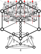
(a)

(b)

Figure 3: Illustration of the crossing gadgets for the proof of Theorem 4.5 in the case $d=7$. (a) A crossing gadget for two edges, one carrying values in $\{1,2\}$ and one in $\{1,3\}$. Observe that simultaneously exchanging the numbers at opposite edges results again in an inner face of size $d$, and this can be done independently for both pairs. (b) A crossing gadget for two edges, one carrying values in $\{1,2\}$ and the other in $\{1,4\}$. The dashed lines show where further gadgets attach, the length of the dotted paths depends on $d$, for $d=7$ their length would be 0.

Figure 4: Illustration of a shift ring consisting of several flow switches. The gray edges on the left and right boundary are identified. The red arrows illustrate the flow of information, where the states of two $(1,2)$-edges carrying different information is transposed in the circular ordering compared to the inner face of the shift ring (above the construction) and the outer face of the shift ring(below the construction).

We are now ready to describe our gadgets. A variable of degree $d$ in $G_{\varphi}^{\prime}$ (recall that $d=2$ or $d=3$), the gadget is a cycle of length $k-d$ such that $d$ edges are $(1,2)$-edges (the output edges) and one is an $(1,d-1)$-edge (the sink edge); see Fig. 2(b) for variable gadgets for $k=7$. Clearly, for the inner face $f$ to have size $k$, either all $(1,2)$-edges must be embedded such that their boundary paths of length 2 are incident to it and the $(1,d-1)$-edge must be embedded such that its boundary path of length 1 is incident to $f$, or all $(1,2)$-edges and the $(1,k-1)$-edge must be flipped. This precisely models the flows emanated by a variable as described above.

We use pipe gadgets to transport flow along an arc. By construction, each arc transports flows from exactly one of the three sets $\{1,2\}$, $\{1,3\}$ and $\{1,4\}$. We give separate pipes for them. Let the set of flow values be $\{1,d\}$. The gadget is a cycle of length $k-d+1$ where two nonadjacent edges are $(1,d)$-edges, one input and one output edge. Clearly, there are $k-d-1$ edges contributing length 1 to the inner face of the gadgets. Thus, the two $(1,d)$-edges must together contribute paths of length $d+1$, which occurs if and only if the information encoded by the input edge is transferred to the output edge.

For a clause of degree $d$ in $G_{\varphi}$ (recall that $d=2$ or $d=3$), the gadget is a cycle of length $k-1$ where $d$ edges are $(1,2)$-edges. Obviously, the inner face $f$ has size $k$ if and only if precisely one of the $(1,2)$-edges has its boundary path of length 2 incident to $f$. Thus, the gadget correctly models a 1-in-3-SAT clause.

For a crossing, one of the two edges transports values in $\{1,2\}$ and the other values in $\{1,3\}$ or in $\{1,4\}$. If it is $\{1,3\}$, we simply use a cycle of length $4$, where two opposite edges are $(1,2)$-edges and the other two opposite edges are $(1,3)$-edges; see Fig. 3(a). From each pair of opposite edges, we designate one as the input edge and one as the output edge. It is not hard to see that the inner face has size $k$ if and only if the state from each input edge is correctly transferred to the output edge. Of course, the same approach could be used for the case $\{1,4\}$, however, this would require $k\geq 8$. Instead, we use a different approach; see Fig. 3(b) for an illustration. First, we split the information into two separate pieces, one that transmits a value in $\{1,2\}$ and one that transmits a value in $\{1,3\}$ (note that the sum of the differences between the upper and the lower values remains constant). Then we cross over the part of the sink edge carrying the flow in $\{1,3\}$ as before. To cross the part of the sink edge carrying flow in $\{1,2\}$ with the variable–clause arc, we use a gadget we call flow switch. It consists of a cycle of length $k-2$ where four edges are $(1,2)$-edges, and for each pair of opposite $(1,2)$-edges one is declared the input and one is the output. Note that, unlike the above crossing gadget, this does not necessarily transfer the input information to the correct output edge. It only requires that half of the $(1,2)$-edges have a boundary path of length 2 in the inner face. However, the fact that, afterwards, we use a symmetric construction as for splitting the flow in $\{1,4\}$ to merge the two flows on the sink edges after the crossing back into a flow in $\{1,4\}$ enforces this behavior.

We can now construct a graph $H_{\varphi}^{\prime}$ by replacing each variable by a variable gadget, each clause by a clause gadget, each crossing by a crossing gadget and each arc by a corresponding pipe gadget. The gadgets are joined to each other by identifying corresponding input and output edges of the gadgets (i.e., we identify the corresponding construction), taking into account the embedding of $G_{\varphi}^{\prime}$. For the sink, we first attach to each of the output edges of the pipe gadgets leading there, a corresponding variable gadget via its sink edge to split the flow arriving there into $(1,2)$-edges. We identify the endpoints of these $(1,2)$-edges such that they form a simple cycle whose interior faces represents the sink.

We now arbitrarily triangulate, possibly by inserting vertices, all faces corresponding to a face of $G_{\varphi}^{\prime}$ that are not internal faces of a gadget and insert into each of the resulting triangles a vertex connected to each triangle vertex by a path of length $(k-1)/2$. This ensures that all resulting subfaces of the triangles have size $k$ and at the same time the embedding of $H_{\varphi}^{\prime}$ is fixed except for the flips of the $(1,d)$-edges. Using the above arguments, it is not hard to see that $\varphi$ admits a satisfying 1-in-3 truth assignment if and only if $H_{\varphi}$ admits a planar embedding where each face has size $k$ except for the face representing the sink vertex, which is bounded by $L$ $(1,2)$-edges and has size $2L-C$. To complete the proof, we present a construction for the interior of the sink that always allows an embedding where all inner faces have size $k$ as long as the outer face has size $2L-C$, i.e., $C$ edges have a boundary path of length 1 at the inner face, and the remaining $L-C$ have a boundary path of length 2 at the inner face.

This works in two steps. First, we build a shift ring, which allows to shift the information encoded in a subset of the edges by one unit to the left or the right. The shift ring consists of a ring of pairs of flow switches as shown in Fig. 4. Its inner and outer face is bounded by $L$ $(1,2)$-edges. There is a natural bijection between the $(1,2)$-edges on the inner and on the outer ring, but the shift ring allows to exchange the state of two adjacent edges. We then nest sufficiently many shift rings ($L^{2}$ certainly suffice), which allows us to assume that, in the innermost face, the edges whose boundary paths have length 2 are consecutive, and the first one (in clockwise direction) is at a specific position. Second, assuming that the innermost face has the configuration of its $(1,2)$-edges as described above, we simply triangulate it arbitrarily and insert into each triangle the construction that makes every face have size $k$. This concludes the construction of the sink gadget, and thus the proof.

Theorem 4.6

$k$-UniformFaces is NP-complete for all even $k\geq 10$.

Proof

The proof runs along the lines of the proof of Theorem 4.5. For this proof, however, we need the additional assumption that number $L$ of literals is even. If it is not the case, we take a variable $x$ that occurs only twice (subdivide an edge to introduce such a variable as in the proof of Theorem 4.4 if none exists). We then create new variables $u,v,w$ and add the clause $(x,u,v)$ and twice the clause $(u,v,w)$. If $x$ has the value true, then setting $u=v=\texttt{false}$ and $w=\texttt{true}$ satisfies the new clauses, and if $x=\texttt{false}$, then $u=\texttt{true}$, $v=w=\texttt{false}$ satisfies them. Thus the resulting formula is equivalent to the original one, has an even number of literals, and satisfies all the conditions of Theorem 4.4.

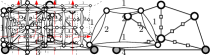
Figure 5: Construction for subdividing a face of even length (bold) into faces of arbitrary size $d$ (here $d=8$).

Now the proof essentially reuses the construction from Theorem 4.5 for such a formula. However, since all faces have to have even size, it is not possible to construct a $(1,2)$-edge (or $(1,k)$-edges with $k$ even for that matter); its outer face would have to have odd length while all interior faces have even length, which is not possible. We thus use $(1,3)$-edges to transmit information for all the gadgets. The sink edges can then use $(1,5)$- and $(1,7)$-edges. A crossing gadget for a $(1,3)$-edge and a $(1,5)$-edge requires a face of size 10. A $(1,7)$-edge can be split into a $(1,3)$ and a $(1,5)$-edge for the corresponding crossing gadget. By choosing suitably long pipes, we can ensure that all faces that are not internal to a gadget have even length. Such a face can then be subdivided into faces of size $d$ by adding a new vertex incident to all vertices of the face and subdividing every second of these edges $d-3$ times; see Fig 5. For the sink, we first distribute the information to $(1,3)$-edges using variable gadgets and then use corresponding shift rings made of flow switches for $(1,3)$-edges. Now, in the innermost face of the shift ring, there are $L$ $(1,3)$-edges of which $C$ have length 1 in the inner face and $L-C$ have length 3, and they can be assumed to be en bloc, starting at a specific edge. The total length of the innermost face then is $3(L-C)+C=3L-2C$, which is even due to our assumption on $L$. Thus, the construction making every face have size $d$ can be done as described above.

Open Problems.

What is the complexity of $k$-UniformFaces for $k=5$ and $k=8$? Are UniformFaces and MinMaxFace polynomial-time solvable for biconnected series-parallel graphs? Are they FPT with respect to treewidth?

Acknowledgments.

We thank Bartosz Walczak for discussions.

References

- [1] P. Angelini, G. Di Battista, and M. Patrignani. Finding a minimum-depth embedding of a planar graph in time. Algorithmica, 60:890–937, 2011.
- [2] D. Bienstock and C. L. Monma. On the complexity of covering vertices by faces in a planar graph. SIAM J. Comput., 17(1):53–76, 1988.
- [3] T. Bläsius, M. Krug, I. Rutter, and D. Wagner. Orthogonal graph drawing with flexibility constraints. Algorithmica, 68:859–885, 2014.
- [4] T. Bläsius, I. Rutter, and D. Wagner. Optimal orthogonal graph drawing with convex bend costs. In F. V. Fomin, R. Freivalds, M. Kwiatkowsak, and D. Peleg, editors, Automata, Languages, and Programming (ICALP’13), volume 7965 of LNCS, pages 184–195. Springer, 2013.
- [5] G. Di Battista, G. Liotta, and F. Vargiu. Spirality and optimal orthogonal drawings. SIAM Journal on Computing, 27(6):1764–1811, 1998.
- [6] G. Di Battista and R. Tamassia. On-line graph algorithms with SPQR-trees. In M. S. Paterson, editor, Automata, Languages and Programming (ICALP’90), volume 443 of LNCS, pages 598–611. Springer, 1990.
- [7] M. R. Fellows, J. Kratochvíl, M. Middendorf, and F. Pfeiffer. The complexity of induced minors and related problems. Algorithmica, 13:266–282, 1995.
- [8] H. N. Gabow. An efficient reduction technique for degree-constrained subgraph and bidirected network flow problems. In Theory of Computing (STOC’83), pages 448–456. ACM, 1983.
- [9] A. Garg and R. Tamassia. On the computational complexity of upward and rectilinear planarity testing. SIAM J. on Comput., 31(2):601–625, 2001.
- [10] C. Gutwenger and P. Mutzel. A linear time implementation of SPQR-trees. In J. Marks, editor, Graph Drawing (GD’00), volume 1984 of LNCS, pages 77–90. Springer, 2001.
- [11] C. Gutwenger and P. Mutzel. Graph embedding with minimum depth and maximum external face (extended abstract). In G. Liotta, editor, Graph Drawing (GD’03), volume 2912 of LNCS, pages 259–272. Springer, 2004.
- [12] C. Moore and J. M. Robson. Hard tiling problems with simple tiles. Discrete Comput. Geom., 26(4):573–590, 2001.
- [13] P. Mutzel and R. Weiskircher. Optimizing over all combinatorial embeddings of a planar graph (extended abstract). In G. Cornuéjols, R. E. Burkard, and G. J. Woeginger, editors, Integer Programming and Combinatorial Optimization (IPCO’99), volume 1610 of LNCS, pages 361–376. Springer, 1999.
- [14] G. J. Woeginger. Embeddings of planar graphs that minimize the number of long-face cycles. Oper. Res. Lett., pages 167–168, 2002.