Adaptive Finite Element Solution of Multiscale PDE-ODE Systems

Abstract

We consider adaptive finite element methods for solving a multiscale system consisting of a macroscale model comprising a system of reaction-diffusion partial differential equations coupled to a microscale model comprising a system of nonlinear ordinary differential equations. A motivating example is modeling the electrical activity of the heart taking into account the chemistry inside cells in the heart. Such multiscale models pose extremely computationally challenging problems due to the multiple scales in time and space that are involved.

We describe a mathematically consistent approach to couple the microscale and macroscale models based on introducing an intermediate “coupling scale”. Since the ordinary differential equations are defined on a much finer spatial scale than the finite element discretization for the partial differential equation, we introduce a Monte Carlo approach to sampling the fine scale ordinary differential equations. We derive goal-oriented a posteriori error estimates for quantities of interest computed from the solution of the multiscale model using adjoint problems and computable residuals. We distinguish the errors in time and space for the partial differential equation and the ordinary differential equations separately and include errors due to the transfer of the solutions between the equations. The estimate also includes terms reflecting the sampling of the microscale model. Based on the accurate error estimates, we devise an adaptive solution method using a “blockwise” approach. The method and estimates are illustrated using a realistic problem.

1 Introduction

Our interest in problems consisting of a macroscale time dependent partial differential equation (PDE) coupled to a miscroscale system of ordinary differential equations (ODEs) originates in the modeling of the electrical activity in the heart. The standard macroscale model of electrical phenomena in cardiac tissue is the bidomain model proposed by Tung [1], which consists of parabolic and elliptic PDEs modeling the macroscopic potential distribution. These PDEs are derived assuming a representation of the tissue as two anisotropic media, one intracellular, which is strongly anisotropic, and one extracellular, which is weakly anisotropic. If the two media are assumed to have proportional conductivity tensors, it is possible to reduce the model to the monodomain model, consisting of a single reaction-diffusion PDE with a load depending on the solution to the ODEs.

On the cellular level, the electrical activity may be modeled by a set of ODEs that depends on a potential determined by the solution of the PDE. Many cellular models are available, both phenomenological models that try to mimic measurements, and physiological models which are based on measurements as well as physiological theory. The latter may be very complex, involving up to hundred variables. For a review on mathematical models describing the electrical activity in the heart, see Sundnes et. al. [2] and the references therein. A space-time adaptive method can be found in Colli Franzone and coworkers [3]. A survey of heart modeling can be found in Noble [4].

Specialized numerical methods are required for high fidelity simulation of the heart, since the heart may consist of up to $10^{10}$ cells [2], each modeled by a set of ODEs, and it is impossible to solve the PDE on the same spatial scale as the ODEs. Moreover, determining the actual physical geometry and location of cells is itself a difficult problem. Thus, including the cellular scale phenomena in the macroscale discretization requires some form of “upscaling” or “recovery” of the information provided by the microscale modeling. This is in fact necessary if the PDE model derived using homogenization as is the case for the bidomain equations.

Unfortunately, this subtle mathematical issue is often ignored in computational electrocardiography, where it is common to simply evaluate the ODEs in the cells located at the quadrature points of a finite element method, for example. However, this is not mathematically consistent, since caused the model to change with the PDE discretization. One consequence, for example, is that it is impossible to perform a mesh convergence study, which is the crudest form of uncertainty quantification.

As an alternative, we create an intermediate “coupling” or “mesoscale” representation of the cellular scale physics that is used to exchange information between the macroscale and microscale. To deal with the very large number of cells, we create the mesoscale representation by sampling cells at the microscale at random and taking averages over the mesoscale cells.

Another potential issue in such coupled systems is significant differences in the temporal scales in the different components. For example, in a system where the ODEs model chemical reactions and the PDE models global behavior such as transport, it is likely that the dynamics of the chemical systems are much faster than that of the total system. Coupled PDE-ODE systems where the ODEs describe chemical reactions and the PDE describe transport occur in applications such as the study of pollution in groundwater, surface water and the atmosphere, control theory and semiconductor simulation. To deal with this, we allow the PDE and ODE systems to employ significantly different time steps.

Numerical solutions of such multiscale systems are invariably affected by error arising from numerous discretization effects and present significant discretization challenges in terms of obtaining a desired accuracy [5]. It is therefore critically important to accurately estimate the numerical error in computed quantities of interest and devise efficient discretization parameter selection algorithms. In this paper, we derive goal-oriented a posteriori error estimates that distinguish the relative contributions of various discretization effects, and thus provide the capability of adjusting various discretization parameters to efficiently obtain a desired accuracy. The error analysis is based on a posteriori error estimates that employ computable residuals and adjoint equations, see [6, 7, 8, 9, 10] for general information. For applications to multiscale systems, see [5, 11, 12, 13, 14, 15, 16]. We base the adaptive strategy on the block adaptive approach described in [17].

The content of this paper is organized as follows: In Section 2, we formulate the multiscale model. In Section 3, we describe the discretization methods. The a posteriori error analysis is presented in Section 4. In Section 5, we describe some implementation details and the adaptive algorithm. A numerical example is presented in Section 6. The paper ends with a conclusion in Section 7.

2 Model description

The nominal model problem consists of a reaction-diffusion PDE that describes macroscale behavior over a domain $\Omega$ coupled to systems of ODEs that model processes taking place inside small “cells” $C$ that comprise the heart domain. The coupling of the macro- and micro-scale processes taking place on vastly different scales in space and time raise serious challenges for analyzing the behavior and computing solutions of the model. We first describe the original coupled system, then we describe a new system that includes a coupling mechanism that provides an avenue to address these challenges.

2.1 The original model

The region $\Omega=\cup_{i=1}^{\mathcal{N}_{C}}C_{i}$ is comprised of $\mathcal{N}_{C}$ cells $C_{i}$ indexed as $\{1,\ldots,\mathcal{N}_{C}\}$. We model the microscale behavior using a collection of ODEs: Find ${\bm{p}}_{i}\in[\mathcal{C}^{1}(0,T)]^{\mathcal{N}_{r}}$ solving

$$\begin{cases}\dot{{\bm{p}}_{i}}={\bm{g}}_{i}(u;{\bm{p}}_{i}),&t\in(0,T],\\ {\bm{p}}_{i}(0)={\bm{p}}_{i}^{0},&\end{cases},\quad i=1,\ldots,\mathcal{N}_{C},$$ (2.1)

where ${\bm{p}}_{i}$ is a vector of length $\mathcal{N}_{r}$ and $u$ is the solution of a PDE modeling the macroscopic behavior described below. In the context of (2.1), $u$ has the role of a parameter. We have allowed the model for the microscale behavior ${\bm{g}}_{i}$ to vary with each cell. For simplicity of notation, we have assumed the same number of equations in each cell model, however this is not necessary.

In order to introduce the microscale solutions of the reactants into the macroscale model, we define the piecewise constant function ${\bm{p}}(x)$ for $x\in\Omega$,

$${\bm{p}}(x,t)={\bm{p}}_{i}(t),\quad(x,t)\in C_{i}\times(0,T],\quad i=1,\ldots,\mathcal{N}_{C}.$$

The macroscale model problem reads: Find $u(x,t)\in\mathcal{C}^{1}((0,T);\mathcal{C}^{2}(\Omega))$ such that

$$\begin{cases}\dot{u}-\nabla\cdot\epsilon\nabla u=f(u;{\bm{p}}),&(x,t)\in\Omega\times(0,T],\\ n\cdot\epsilon\nabla u=0,&(x,t)\in\partial\Omega\times(0,T],\\ u(x,0)=u^{0}(x),&x\in\Omega,\end{cases}$$ (2.2)

where $\epsilon=\epsilon(x)\geq\epsilon_{0}>0$ is a continuous function and $f$ and $u^{0}$ are sufficiently smooth functions. In this equation, ${\bm{p}}$ now plays the role of a parameter, but one that varies in space on the microscale.

2.2 Multiscale coupling

The coupled system (2.1)-(2.2) immediately raises several issues:

• The solutions of the microscale ODEs (2.1) vary in space on the scale of the cells. This happens both because of varying cell model and because the ODE model (2.1) depend on experimentally-determined parameters that vary stochastically. This microscale variation introduces extremely rapid variation in the coefficient $f$ on the scale of the macroscale PDE (2.2) along with discontinuities across cell boundaries. We would therefore have to use a spatial discretization for (2.2) that is finer than the cells while being consistent with the cell boundaries in order to achieve full order accuracy in numerical solutions.

• The ODE system (2.1) has an extremely large dimension $\mathcal{N}_{C}\times\mathcal{N}_{r}$, with the consequence that the solution of many systems of nonlinear ODEs are required to advance the PDE solution if we solve the microscale model (2.1) in every cell. This raises another significant computational burden.

• At the same time, we expect to see a macroscale pattern in variations in cell type and model, which implies it is inefficient to integrate the microscale ODEs in every cell.

To deal with these issues, we introduce a coupling scale decomposition of $\Omega$. We assume that $\Omega=\cup_{j=1}^{\mathcal{N}_{\omega}}\omega_{j}$ is decomposed into a set of non-overlapping regions $\omega_{i}$. Each $\omega_{j}$ is comprised of a collection of cells $\omega_{j}=\cup_{i\in\mathcal{I}_{j}}C_{i}$, where $\mathcal{I}_{j}$ is a subset of the indices $\{1,\ldots,\mathcal{N}_{C}\}$. We assume the collection $\{\mathcal{I}_{j}\}$ is non-intersecting while their union equals $\{1,\ldots,\mathcal{N}_{C}\}$. To smooth out the cell-scale variation in the reaction model (2.1), we average the reaction solutions over $\omega_{i}$. We introduce a “recovery” operator $\mathcal{R}:\mathbb{R}^{\mathcal{N}_{C}\times\mathcal{N}_{r}}\to[\mathcal{L}^{2}(\Omega)]^{\mathcal{N}_{r}}$ defined as

$$\mathcal{R}{\bm{p}}(x)=\frac{1}{|\omega_{j}|}\int_{\omega_{j}}{\bm{p}}(y)\,dy=\frac{1}{|\omega_{j}|}\left(\sum_{i\in\mathcal{I}_{j}}{\bm{p}}_{i}|C_{i}|\right),\quad x\in\omega_{j},\quad j=1,\ldots,\mathcal{N}_{\omega},$$ (2.3)

where $|\omega_{j}|$ and $|C_{i}|$ denote the volume of the indicated region and cell respectively. Note that $\sum_{i\in\mathcal{I}_{j}}|C_{i}|=|\omega_{j}|$. The function $\mathcal{R}{\bm{p}}$ is piecewise constant, but now varies on the coupling scale rather than the cell scale.

One reasonable criteria to choosing the intermediate scale cells is to assume that the same reaction model ${\bm{g}}_{i}$ is used for each cell $C_{i}$ in each coupling region $\omega_{j}$. We now replace the original macroscale model problem (2.2) by

$$\begin{cases}\dot{u}-\nabla\cdot\epsilon\nabla u=f(u;\mathcal{R}{\bm{p}}),&(x,t)\in\Omega\times(0,T],\\ n\cdot\epsilon\nabla u=0,&(x,t)\in\partial\Omega\times(0,T],\\ u(x,0)=u^{0}(x),&x\in\Omega,\end{cases}$$ (2.4)

Next we note that in the original formulation, ${\bm{p}}_{i}$ depends implicitly on the spatial variable $x$ (which has the role of a parameter) inside each cell. To avoid this, we introduce a projection of $u$ into a space of functions that are constant on each cell. We let $\mathcal{P}:\mathcal{L}^{2}(\Omega)\to\mathbb{R}^{\mathcal{N}_{C}}$ be a suitably chosen projection into functions that are piecewise constant on the cells and we replace (2.1) by

$$\begin{cases}\dot{{\bm{p}}_{i}}={\bm{g}}_{i}(\mathcal{P}u;{\bm{p}}_{i}),&t\in(0,T],\\ {\bm{p}}_{i}(0)={\bm{p}}_{i}^{0},&\end{cases}\quad i=1,\ldots,\mathcal{N}_{C},$$ (2.5)

When the exact spatial location of each cell is unavailable, as often is the case, we use a projection $\mathcal{P}$ into the space of functions that are constant on the coupling scale domains $\omega_{j}$, which also produces a function that is constant on each cell.

3 Multirate finite element methods

In order to derive a variational a posteriori error estimate, we write the time discretization as a finite element method for a piecewise polynomial while using a common finite element method for spatial discretization. Combined with suitable quadrature formulas, the resulting approximations match standard finite difference schemes.

3.1 Variational formulation

To this end, we let $(\cdot,\cdot)_{X}$ denote the inner product on $\mathcal{L}^{2}(X)$ on a space $X$ with corresponding norm $\lVert\cdot\rVert_{X}$ and let $a(v,w)$ denote the bilinear form $a(v,w)_{X}=(\epsilon\nabla v,\nabla w)_{X}$. The subscript $X$ is dropped when $X=\Omega$. Furthermore, we let $\langle\cdot,\cdot\rangle_{C_{j}}$ denote the inner product on $\mathbb{R}^{\mathcal{N}_{r}}$ on cell $C_{j}$ and let $\langle\cdot,\cdot\rangle=\sum_{i=1}^{\mathcal{N}_{C}}\langle\cdot,\cdot\rangle_{C_{i}}$. The corresponding norm is denoted by $\lVert\cdot\rVert$, which is the same notation as for the $\mathcal{L}^{2}$-norm, but it is obvious from the context which norm is intended. Furthermore, we write the right hand side functions $f$ and ${\bm{g}}$ as functions of two variables, replacing ’;’ with ’,’.

We first write (2.5)-(2.4) in variational form: The solutions ${\bm{p}}_{i}\in[\mathcal{H}^{1}(0,T)]^{\mathcal{N}_{r}}$ of (2.5) satisfy,

$$\int_{0}^{T}\langle\dot{{\bm{p}}}_{i},{\bm{q}}\rangle\ dt=\int_{0}^{T}\langle{\bm{g}}_{i}(\mathcal{P}u,{\bm{p}}_{i}),{\bm{q}}\rangle\ dt,\quad\forall{\bm{q}}\in[\mathcal{L}^{2}(0,T)]^{\mathcal{N}_{r}},\;\quad i=1,\ldots,\mathcal{N}_{C},$$ (3.1)

while the solution $u\in\mathcal{L}^{2}((0,T);\mathcal{H}^{1}(\Omega))$ satisfies,

$$\int_{0}^{T}(\dot{u},v)+a(u,v)\ dt=\int_{0}^{T}(f(u,{\mathcal{R}}{\bm{p}}),v)\ dt,\quad\forall v\in\mathcal{L}^{2}((0,T);\mathcal{H}^{1}(\Omega)).$$ (3.2)

3.2 A multirate finite element method

We solve the coupled system (2.5)-(2.4) using a discretization that allows different time steps to be used for the ODEs and the PDE. The discretization yields a nonlinear coupled system of discrete equations for the approximate solution that must be solved iteratively in practice. It is common to fix the number of iterations used for such coupled systems, which can significantly affect the properties of the resulting numerical solution. In the extreme case with no iteration, this represents a so-called explicit-implicit scheme.

For the temporal discretization for the PDE, the time interval $[0,T]$ is partitioned into $N$ subintervals $0=t_{0}<t_{1}<\cdots<t_{N}=T$, and we denote each subinterval by $I_{n}=(t_{n-1},t_{n}]$ with length by $\Delta t_{n}=t_{n}-t_{n-1}$. For the temporal mesh for the ODEs, each interval $I_{n}$ may be divided into $M_{n}$ subintervals by $t_{n-1}=s_{0,n}<s_{1,n}<\cdots<s_{M_{n},n}=t_{n}$, where $J_{m,n}=(s_{m-1,n},s_{m,n}]$ and is of length $\Delta s_{m,n}=s_{m,n}-s_{m-1,n}$. This is illustrated in Fig. 3.1. We also allow for different time steps in different cells, but the notation becomes very cumbersome so we do not indicate this. Moreover, we note that it is possible to let the individual $\mathcal{N}_{r}$ ODE components have different time stepping as in [13], but this is not considered here.

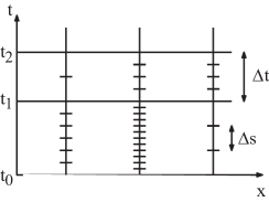
Figure 3.1: The PDE time steps $\Delta t$ (long horizontal lines) is allowed to depend on $t$ but not on $x$. The ODE time steps $\Delta s$ (short horizontal lines) may depend on both $t$ and $x$.

The space of polynomials of order $r$ is denoted $\mathbb{P}^{r}$, and we discretize all the $\mathcal{N}_{r}$ ODE components in the space of polynomials of degree $r_{p}$, $\bm{\mathcal{Q}}_{m,n}^{r_{p}}=\{{\bm{q}}(t):{\bm{q}}|_{I_{m,n}}\in[\mathbb{P}^{r_{p}}(I_{m,n})]^{\mathcal{N}_{r}}\}$. We denote the space of functions $\cup_{m=1}^{M_{n}}\bm{\mathcal{Q}}_{m,n}^{r_{p}}$ by $\bm{\mathcal{Q}}_{n}^{r_{p}}$. To simplify notation, we use the same order of polynomial in all cells, though this is not necessary.

For the PDE, we define a triangulation $\mathcal{T}_{n}^{h}$ of $\Omega$ on each interval $I_{n}$ that is inconsistent with the coupling scale decomposition $\Omega=\cup_{j=1}^{\mathcal{N}_{\omega}}\omega_{j}$: We let $\mathcal{T}_{n}^{h}$ be hexahedral elements and let the coupling scale partition be the Voronoi tessellation defined by $\mathcal{N}_{\omega}$ uniformly distributed random points in $\Omega$, i.e. each $\omega_{j}$ is a Voronoi cell [18]. An illustration of this tessellation can be seen in Fig. 3.2.

Let $\mathcal{V}_{n}^{h}\subset\mathcal{H}^{1}(\Omega)$ be the space $\mathcal{V}_{n}^{h}=\{v(x)\in\mathcal{C}(\Omega):v|_{K}\in\mathbb{P}^{r}(K),\ K\in\mathcal{T}_{n}^{h}\}$. To indicate the sizes of the elements in $\mathcal{V}_{n}^{h}$, we introduce the mesh function $h_{K}=\text{diam}(K)$ for $K\in\mathcal{T}_{n}^{h}$ and $h=\max h_{K}$. The approximation is in the space-time function space $\mathcal{W}^{r_{u}}_{n}=\{w(x,t):w(x,t)=\sum_{i=0}^{r_{u}}t^{i}v_{i}(x),\ v_{i}\in\mathcal{V}_{n}^{h},\ (x,t)\in\Omega\times I_{n}\}$.

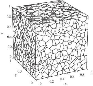
Figure 3.2: Illustration of a Voronoi tessellation with $\mathcal{N}_{\omega}=4096$.

The functions in $\mathcal{W}^{r_{u}}_{n}$ and $\bm{\mathcal{Q}}^{r_{p}}_{n}$ are discontinuous at time nodes, and we denote the jump across a time nodes $t_{i}$ by $[v]_{i}=v_{i}^{+}-v_{i}^{-}$, where $v_{i}^{\pm}=\lim_{t\rightarrow t_{i}^{\pm}}v(t)$. Finally in order to evaluate Galerkin orthogonality, we use the following projection operators into the discrete spaces:

$$\Pi_{n} :\mathcal{L}^{2}(\Omega)\rightarrow\mathcal{V}_{n}^{h},$$ (3.3)

$$\pi_{n}^{u} :\mathcal{L}^{2}(I_{n})\rightarrow\mathbb{P}^{r_{u}}(I_{n}),$$ (3.4)

$${\bm{\pi}}_{m,n}^{p} :[\mathcal{L}^{2}(I_{m,n})]^{\mathcal{N}_{r}}\rightarrow[\mathbb{P}^{r_{p}}(I_{m,n})]^{\mathcal{N}_{r}}.$$ (3.5)

Note that $\pi_{n}^{u}\Pi_{n}=\Pi_{n}\pi_{n}^{u}:\mathcal{L}^{2}(\Omega\times I_{n})\rightarrow\mathcal{W}^{r_{u}}_{n}$.

The multirate finite element method now reads: For all cells in $C$ and for each time interval $n=1,\ldots,N$, find ${\bm{P}}\in\bm{\mathcal{Q}}_{m,n}^{r_{p}}$ for $m=1,\ldots,M_{n}$ such that

$$\int_{I_{m,n}}\langle\dot{{\bm{P}}},{\bm{q}}\rangle\ dt+\langle[{\bm{P}}]_{m-1,n},{\bm{q}}^{+}\rangle=\int_{I_{m,n}}\langle{\bm{g}}(\mathcal{P}U,{\bm{P}}),{\bm{q}}\rangle\ dt,\quad\forall{\bm{q}}\in\bm{\mathcal{Q}}_{m,n}^{r_{p}},$$ (3.6)

with ${\bm{P}}^{0-}={\bm{p}}^{0}$. Note that there are $\mathcal{N}_{C}$ ODE systems in (3.6). The PDE discretization is: Find $U\in\mathcal{W}^{r_{u}}_{n}$ such that

$$\int_{I_{n}}(\dot{U},v)+a(U,v)\ dt+([U]_{n-1},v^{+}) =\int_{I_{n}}(f(U,{\mathcal{R}}{\bm{P}}),v)\ dt,\quad\forall v\in\mathcal{W}^{r_{u}}_{n},$$ (3.7)

where $U_{0}^{-}=\Pi_{0}u^{0}$.

Note that if we use $r_{p}=r_{u}=0$ with a left-hand rectangle rule for time integrals and employ a standard “lumped-mass” quadrature rule in space (trapezoidal rule on elements), then we obtain a standard difference approximation consisting of the implicit Euler in time and 5 point stencil difference scheme in space [8].

3.3 Practical discretization considerations

There are additional considerations for discretization that are used in practice.

Evaluation of the recovery operator

The definition of the recovery operator $\mathcal{R}$ in (2.3) requires the solution of the cell reaction equations (2.5) on all $\mathcal{N}_{C}$ cells. We expect $\mathcal{N}_{C}$ to be very large, e.g. on the order of millions to billions. At the same time, we expect that the physical properties of cells vary over the macroscale rather than microscale, so it is inefficient to solve (2.5) on every cell. We approximate $\mathcal{R}$ by an average $\widetilde{\mathcal{R}}$ computed using a Monte Carlo sampling approach with a (relatively small) sample of the problems (2.5). As a consequence, we replace the PDE equation (3.7) by: Find $U\in\mathcal{W}^{r_{u}}_{n}$ such that

$$\int_{I_{n}}(\dot{U},v)+a(U,v)\ dt+([U]_{n-1},v^{+})=\int_{I_{n}}(f(U,\widetilde{\mathcal{R}}{\bm{P}}),v)\ dt,\quad\forall v\in\mathcal{W}^{r_{u}}_{n},$$ (3.8)

where $U_{0}^{-}=\Pi_{0}u^{0}$.

There are two ways to compute the samples. First, we can sample in the spatial variable $x$, so for $x\in\omega_{j}$,

$$\widetilde{\mathcal{R}}{\bm{p}}(x)=\frac{1}{K_{j}}\sum_{k=1}^{K_{j}}{\bm{p}}(x_{j,k}),$$ (3.9)

where $\{x_{j,k}\}_{k=1}^{K_{j}}$ is a set of $K_{j}$ points chosen at random in $\omega_{j}$, for each $j=1,\ldots,\mathcal{N}_{\omega}$. In this approach, we solve the reaction model (2.5) only in cells located at $\{x_{j,k}\}_{k=1}^{K_{j}}$. This means that the average is affected by by physical size of the cells, since bigger cells contribute more samples with some probability. Alternatively, we can sample by choosing cell indices at random, so for $x\in\omega_{j}$,

$$\widetilde{\mathcal{R}}{\bm{p}}(x)=\frac{1}{K_{j}}\sum_{k=1}^{K_{j}}{\bm{p}}_{i_{k}},$$ (3.10)

where $\{i_{k}\}$ is a randomly selected subset of $\mathcal{I}_{j}$. In the second approach, the cell average is not affected by the size of the cell.

Note that this Monte Carlo computation has the property that the computation is actually exact if sufficiently many samples are used, since there are only $\mathcal{N}_{C}$ different values. However for very large $\mathcal{N}_{C}$ and reasonably small numbers of samples, the convergence of the Monte Carlo approximations appears to behave according to the standard asymptotic results, so that the accuracy is roughly proportional to the variance of the integrand divided by the square root of the number of samples. Since we want to use relatively few samples, this indicates that the coupling regions $\omega_{j}$ should be chosen so that the variance of the integrand defining $\mathcal{R}$ has small variance.

Iterative solution of the nonlinear discrete equations

In general, (3.6)-(3.8) presents a nonlinear coupled discrete system that is solved iteratively in practice. We describe a simple fixed point iteration.

We use the superscript $\ell$ to denote the iteration number and assume that we carry out $L_{n}$ total iterations on each time step. In practice, we may vary the number of iterations in each cell and for the PDE, but we suppress that notation. The fixed point - finite element method can be formulated on time interval $I_{n}$ as: Given ${\bm{P}}^{0}={\bm{P}}(t_{n-1})$ and $U^{0}=U(x,t_{n-1})$, for each cell find ${\bm{P}}^{\ell}\in\bm{\mathcal{Q}}_{m,n}^{r_{p}}$ for $m=1,\dots,M_{n}$ on $I_{n}$ such that

$$\int_{I_{m,n}}\langle\dot{{\bm{P}}^{\ell}},{\bm{q}}\rangle\ dt+\langle({\bm{P}}^{\ell+}-{\bm{P}}^{-})|_{m-1,n},{\bm{q}}^{+}_{m-1,n}\rangle=\\ \int_{I_{m,n}}\langle{\bm{g}}(\mathcal{P}U^{\ell-1},{\bm{P}}^{\ell}),{\bm{q}}\rangle\ dt,\quad\forall{\bm{q}}\in\bm{\mathcal{Q}}_{m,n}^{r_{p}}.$$ (3.11)

Then, given ${\bm{P}}^{\ell}$ on $I_{n}$, find $U^{\ell}\in\mathcal{W}^{r_{u}}_{n}$ such that

$$\int_{I_{n}}(\dot{U}^{\ell},v)+a(U^{\ell},v)\ dt+((U^{\ell+}-U^{-})|_{n-1},v^{+}_{n-1})\\ =\int_{I_{n}}(f(U^{\ell},\widetilde{\mathcal{R}}{\bm{P}}^{\ell}),v)\ dt,\quad\forall v\in\mathcal{W}^{r_{u}}_{n},$$ (3.12)

given $U^{0}$. We iterate (3.11) and (3.12) for $\ell=1,\ldots,L_{n}$, set ${\bm{P}}^{-}_{n}={\bm{P}}^{L_{n}}(t_{n})$ and $U^{-}_{n}=U^{L_{n}}(t_{n})$ to form the data for the next interval.

In this iterative formulation, we are “lagging” the values of the PDE model $U$ in the cell reaction model, but treat the remaining nonlinear problems for ${\bm{P}}^{\ell}$ and $U^{\ell}$ implicitly. This entails using an additional nonlinear solver for each model equation. However, we do not indicate this in the notation as these problems can typically be solved very accurately, e.g. using a standard Newton method.

An implicit-explicit method

In practice, the iterative formulation (3.11)-(3.12) is often solved for only one iteration $L_{n}=1$, yielding an “implicit-explicit” method. This is: For $n=1,\ldots,N$, find ${\bm{P}}\in\bm{\mathcal{Q}}_{m,n}^{r_{p}}$ for $m=1,\ldots,M_{n}$ such that

$$\int_{I_{m,n}}\langle\dot{{\bm{P}}},{\bm{q}}\rangle\ dt+\langle[{\bm{P}}]_{m-1,n},{\bm{q}}^{+}\rangle=\int_{I_{m,n}}\langle{\bm{g}}(\mathcal{P}U_{n-1},{\bm{P}}),{\bm{q}}\rangle\ dt,\quad\forall{\bm{q}}\in\bm{\mathcal{Q}}_{m,n}^{r_{p}},$$ (3.13)

with ${\bm{P}}^{0-}={\bm{p}}^{0}$. Then find $U\in\mathcal{W}^{r_{u}}_{n}$ such that

$$\int_{I_{n}}(\dot{U},v)+a(U,v)\ dt+([U]_{n-1},v^{+})=\int_{I_{n}}(f(U,\widetilde{\mathcal{R}}{\bm{P}}),v)\ dt,\quad\forall v\in\mathcal{W}^{r_{u}}_{n},$$ (3.14)

where $U_{0}^{-}=\Pi_{0}u^{0}$. The scheme is said to be explicit-implicit due to the use of explicit use of $U_{n-1}$ when solving for ${\bm{P}}$ on $I_{n}$, while $U_{n}$ is solved implicitly.

4 A posteriori error analysis

In this section, we derive adjoint-based error representation formulas for the methods above. Using these formulas, we derive indicators of local contributions to the global error that can serve as the basis for an adaptive method. Ignoring the effect of iteration in the solution of the discrete equations, there are three discretization parameters that affec the numerical accuracy, namely the spatial mesh size, the time steps for the PDE, and the time steps for the ODEs. In addition, there is a choice of the projection and recovery operators. We present error indicators that distinguish the relative contributions of these choices to the global error. For the iterative method, there is the additional parameter of number of iterations per time step.

We begin by noting that since the right hand side of (3.13) involves the solution $U_{n-1}$ from the previous time step and since the right hand side of (3.14) involves the approximation $\widetilde{\mathcal{R}}$, there is an error arising from operator decomposition [5] due the differences $U$ and $U_{n-1}$ as well as a modeling error due to the differences between $\mathcal{R}$ and $\widetilde{\mathcal{R}}$.

4.1 Preliminaries

The adjoint to the function spaces presented is denoted by the superscript $*$. The same notation is used for the adjoint operators, as noted in the following identities

$$(v,\mathcal{R}{\bm{q}}) =\langle\mathcal{R}^{*}v,{\bm{q}}\rangle,$$ (4.1)

$$\langle\mathcal{P}v,{\bm{q}}\rangle =(v,\mathcal{P}^{*}{\bm{q}}),$$ (4.2)

which hold for any ${\bm{q}}\in\bm{\mathcal{Q}}_{m,n}^{r_{p}}$ and $v\in\mathcal{W}_{n}^{r_{u}}$.

We define the residuals, the linearizations of the functions $f$ and ${\bm{g}}$ and state the adjoint problems. The derivation of the theorems follow in the next Section.

Definition 4.1.

Let the residuals corresponding to (3.13) and (3.14) be denoted by ${\bm{R}}_{p}({\bm{P}})\in\bm{\mathcal{Q}}_{m,n}^{r_{p}*}$ and $R_{u,K}(U,{\bm{P}})\in\mathcal{W}^{r_{u}*}_{n}$. These are defined by

$$\int_{I_{m,n}}\langle{\bm{R}}_{p}({\bm{P}}),{\bm{q}}\rangle\ dt =\int_{I_{m,n}}\langle{\bm{g}}(\mathcal{P}U_{n-1},{\bm{P}})-\dot{{\bm{P}}},{\bm{q}}\rangle\ dt-\langle[{\bm{P}}]_{m-1,n},{\bm{q}}_{m-1,n}^{+}\rangle,$$ (4.3)

$$\int_{I_{n}}(R_{u,K}(U,{\bm{P}}),v)_{K}\ dt =\int_{I_{n}}(f(U,\widetilde{\mathcal{R}}{\bm{P}})-\dot{U}+\nabla\cdot\epsilon\nabla U,v)_{K}$$

$$\qquad-\frac{1}{2}([n\cdot\epsilon\nabla U],v)_{\partial K\setminus\partial\Omega}\ dt-([U]_{n-1},v_{n-1}^{+})_{K}.$$ (4.4)

Definition 4.2.

The linearizations of $f$ and ${\bm{g}}$ are defined as

$$\overline{f_{u}} =\int_{0}^{1}\frac{\partial f}{\partial u}(us+U(1-s),\mathcal{R}{\bm{p}}s+\mathcal{R}{\bm{P}}(1-s))\ ds,$$ (4.5)

$$\overline{{\bm{f}}_{p}} =\left[\int_{0}^{1}\frac{\partial f}{\partial\mathcal{R}{\bm{p}}_{j}}(us+U(1-s),\mathcal{R}{\bm{p}}s+\mathcal{R}{\bm{P}}(1-s))\ ds\right]_{j=1}^{\mathcal{N}_{r}},$$ (4.6)

$$\overline{{\bm{g}}_{u}} =\left[\int_{0}^{1}\frac{\partial{\bm{g}}_{i}}{\partial\mathcal{P}u}(\mathcal{P}us+\mathcal{P}U(1-s),{\bm{p}}s+{\bm{P}}(1-s))\ ds\right]_{i=1}^{\mathcal{N}_{r}},$$ (4.7)

$$\overline{{\bm{g}}_{p}} =\left[\int_{0}^{1}\frac{\partial{\bm{g}}_{i}}{\partial{\bm{p}}_{j}}(\mathcal{P}us+\mathcal{P}U(1-s),{\bm{p}}s+{\bm{P}}(1-s))\ ds\right]_{i,j=1}^{\mathcal{N}_{r}}.$$ (4.8)

4.2 Adjoint problems

The definition of an appropriate adjoint problem for a multiscale model is a problematic issue [5]. First of all, there are a number of possible adjoint problems that can be associated with any nonlinear differential equation. In addition, it may be reasonable to account for the use of projections between scales and representations and the effects of a finite number of iterations in the definition. Another issue is the computational difficulty and cost required in the numerical solution of the adjoint.

We consider two different adjoint problems that present a tradeoff between accuracy of the resulting estimates on one hand and the cost and practicality of implementation on the other. The first approach is closely related to the ideal adjoint of the coupled system (3.1)-(3.2) treated by an implicit discretization, a so-called “implicit adjoint”. This choice leads to a robustly accurate error estimate, but the cost is that the linear adjoint problem is nearly as difficult to solve numerically as the original multiscale model. As an alternative, we define a second adjoint problem that uses the same decomposition and finite iterations as used in the forward model. This approach is much more computationally tractable, however the resulting error estimate includes terms that cannot be estimated. It is possible to show that these terms are relative small compared to the terms that can be estimated in the limit of refined discretization however.

4.3 Fully implicit adjoint problem and error representation formula

The ideal fully implicit adjoint reads: For $n=N,\ldots,1$, find $\widetilde{\bm{\phi}}_{p}(t)\in[\mathcal{L}^{2}(I_{m,n})]^{\mathcal{N}_{r}}$ on $m=1,\ldots,M_{n}$ and $\widetilde{\phi}_{u}(x,t)\in\mathcal{L}^{2}(I_{n};\mathcal{H}^{1}(\Omega))$ such that

$$\int_{I_{m,n}}\langle{\bm{q}},-\dot{\widetilde{{\bm{\phi}}}}_{p}\rangle-\langle{\bm{q}},\overline{{\bm{g}}_{p}}^{*}\widetilde{\bm{\phi}}_{p}+\mathcal{R}^{*}\overline{{\bm{f}}_{p}}^{*}\widetilde{\phi}_{u}\rangle\ dt =\int_{I_{m,n}}\langle{\bm{q}},{\bm{\psi}}_{p}\rangle\ dt$$ (4.9)

and

$$\int_{I_{n}}(v,-\dot{\widetilde{\phi}}_{u})+a(v,\widetilde{\phi}_{u})-(v,\overline{f_{u}}^{*}\widetilde{\phi}_{u}+\mathcal{P}^{*}\overline{g_{u}}^{*}\widetilde{\bm{\phi}}_{p})\ dt =\int_{I_{n}}(v,\psi_{u})\ dt,$$ (4.10)

where $\psi_{u}\in\mathcal{L}^{2}(\Omega)$ and ${\bm{\psi}}_{p}\in[\mathcal{L}^{2}(\Omega)]^{\mathcal{N}_{r}}$ are given data that determine the quantity of interest to be computed. The initial conditions for the adjoint problem are $\widetilde{\phi}_{u}(x,T)=0$ and $\widetilde{\bm{\phi}}_{p}(T)=\mathbf{0}$. Next we derive the error representation formula corresponding to this fully implicit adjoint problem.

Theorem 4.1 (Error representation formula).

Let the quantity of interest be the linear functional $m(u,{\bm{p}})$ be defined by the functions $\psi_{u}\in\mathcal{L}^{2}(\Omega)$ and ${\bm{\psi}}_{p}\in[\mathcal{L}^{2}(\Omega)]^{\mathcal{N}_{r}}$ such that $m(u,{\bm{p}})=\int_{0}^{T}(u,\psi_{u})+\langle{\bm{p}},{\bm{\psi}}_{p}\rangle\ dt$. The error representation formula for the error $E(U,{\bm{P}})=\lvert m(u,{\bm{p}})-m(U,{\bm{P}})\rvert$ reads

$$E(U,{\bm{P}}) =\Big{|}\sum_{n=1}^{N}\int_{I_{n}}(e_{u},\psi_{u})+\langle{\bm{e}}_{p},{\bm{\psi}}_{p}\rangle\ dt\Big{|}$$ (4.11)

$$=\Big{|}I+\sum_{n=1}^{N}(II_{n}+III_{n}+IV_{n}+V_{n}+V\!I_{n})\Big{|},$$ (4.12)

where

$$I =(u^{0}-\Pi_{0}u^{0},\widetilde{\phi}_{u,0}),$$ (4.13)

$$II_{n} =\sum_{K\in\mathcal{T}_{n}^{h}}\int_{I_{n}}(R_{u,K}(U,{\bm{P}}),\widetilde{\phi}_{u}-\Pi_{n}\pi_{n}^{u}\widetilde{\phi}_{u})_{K}\ dt,$$ (4.14)

$$III_{n} =\sum_{m=1}^{M_{n}}\int_{I_{m,n}}\langle{\bm{R}}_{p}({\bm{P}}),\widetilde{\bm{\phi}}_{p}-{\bm{\pi}}_{m,n}^{p}\widetilde{\bm{\phi}}_{p}\rangle\ dt,$$ (4.15)

$$IV_{n} =\int_{I_{n}}(f(U,\mathcal{R}{\bm{P}})-f(U,\widetilde{\mathcal{R}}{\bm{P}}),\widetilde{\phi}_{u})\ dt,$$ (4.16)

$$V_{n} =\int_{I_{n}}\langle{\bm{g}}(\mathcal{P}U,{\bm{P}})-{\bm{g}}(\mathcal{P}U_{n-1},{\bm{P}}),\widetilde{\bm{\phi}}_{p}\rangle\ dt.$$ (4.17)

The first term is the contribution from error in the initial data for the PDE. The second and the third terms quantify the contributions of the discretization of the PDE and the ODEs respectively. The fourth term quantifies the contribution of the recovery operator and the fifth term is the contribution of the explicit splitting scheme.

Proof.

Introducing the errors $e_{u}=u-U$ and ${\bm{e}}_{p}={\bm{p}}-{\bm{P}}$, we use the chain rule identities to obtain,

$$\langle\overline{{\bm{g}}_{u}}\mathcal{P}e_{u}+\overline{{\bm{g}}_{p}}{\bm{e}}_{p},{\bm{q}}\rangle =\langle{\bm{g}}(\mathcal{P}u,{\bm{p}})-{\bm{g}}(\mathcal{P}U,{\bm{P}}),{\bm{q}}\rangle,$$ (4.18)

$$(\overline{f_{u}}e_{u}+\overline{{\bm{f}}_{p}}\mathcal{R}{\bm{e}}_{p},v) =(f(u,\mathcal{R}{\bm{p}})-f(U,\mathcal{R}{\bm{P}}),v).$$ (4.19)

Note that (4.18) holds on each $I_{m,n}$ whereas (4.19) holds on each $I_{n}$. Furthermore, by the continuity of $u$,

$$e_{u,(m-1,n)}^{+} =u_{m-1,n}^{+}-U_{m-1,n}^{+}=(u_{m-1,n}^{-}-U_{m-1,n}^{-})-(U_{m-1,n}^{+}-U_{m-1,n}^{-})$$ (4.20)

$$=e_{u,(m-1,n)}^{-}-[U]_{m-1,n}.$$

Similarly,

$${\bm{e}}_{p,(m-1,n)}^{+} ={\bm{e}}_{p,(m-1,n)}^{-}-[{\bm{P}}]_{m-1,n}.$$ (4.21)

Now substituting ${\bm{e}}_{p}$ for ${\bm{q}}$ in (4.9) and applying integration by parts we arrive at,

$$\int_{I_{m,n}}\langle{\bm{e}}_{p},{\bm{\psi}}_{p}\rangle\ dt =\int_{I_{m,n}}\langle{\bm{e}}_{p},-\dot{\widetilde{{\bm{\phi}}}}_{p}\rangle-\langle{\bm{e}}_{p},\overline{{\bm{g}}_{p}}^{*}\widetilde{\bm{\phi}}_{p}+\mathcal{R}^{*}\overline{{\bm{f}}_{p}}^{*}\widetilde{\phi}_{u}\rangle\ dt$$ (4.22)

$$=-\langle{\bm{e}}_{p}^{-},\widetilde{\bm{\phi}}_{p}\rangle_{m-1,n}+\langle{\bm{e}}_{p}^{+},\widetilde{\bm{\phi}}_{p}\rangle_{m-1,n}$$

$$\phantom{a}\quad+\int_{I_{m,n}}\langle{\dot{{\bm{e}}}}_{p},\widetilde{\bm{\phi}}_{p}\rangle-\langle\overline{{\bm{g}}_{p}}{\bm{e}}_{p},\widetilde{\bm{\phi}}_{p}\rangle\ dt-\int_{I_{m,n}}\langle\overline{{\bm{f}}_{p}}\mathcal{R}{\bm{e}}_{p},\widetilde{\phi}_{u}\rangle\ dt$$

Now we apply (4.21),

$$\int_{I_{m,n}}\langle{\bm{e}}_{p},{\bm{\psi}}_{p}\rangle\ dt =-\langle{\bm{e}}_{p}^{-},\widetilde{\bm{\phi}}_{p}\rangle_{m,n}+\langle{\bm{e}}_{p}^{-},\widetilde{\bm{\phi}}_{p}\rangle_{m-1,n}-\langle[{\bm{P}}]_{m-1,n},\widetilde{\bm{\phi}}_{p,(m-1,n)}\rangle$$ (4.23)

$$\phantom{a}\quad+\int_{I_{m,n}}\langle{\dot{{\bm{e}}}}_{p},\widetilde{\bm{\phi}}_{p}\rangle-\langle\overline{{\bm{g}}_{p}}{\bm{e}}_{p},\widetilde{\bm{\phi}}_{p}\rangle-\langle\overline{{\bm{f}}_{p}}\mathcal{R}{\bm{e}}_{p},\widetilde{\phi}_{u}\rangle\ dt.$$

A similar computation for $e_{u}$ leads to,

$$\int_{I_{n}}(e_{u},\psi_{u})\ dt =-(e_{u}^{-},\widetilde{\phi}_{u})_{n}+(e_{u}^{-},\widetilde{\phi}_{u})_{n-1}-([U]_{n-1},\widetilde{\phi}_{u,(n-1)})$$ (4.24)

$$+\int_{I_{n}}(\dot{e}_{u},\widetilde{\phi}_{u})+a(e_{u},\widetilde{\phi}_{u})-(\overline{f_{u}}e_{u},\widetilde{\phi}_{u})-(\overline{g_{u}}\mathcal{P}e_{u},\widetilde{\bm{\phi}}_{p})\ dt$$ .

Summing (4.23) over all $m$, combining it with (4.24) and using (4.18) and (4.19) leads to,

$$\int_{I_{n}}(e_{u},\psi_{u}) +\langle{\bm{e}}_{p},{\bm{\psi}}_{p}\rangle\ dt=-\langle{\bm{e}}_{p}^{-},\widetilde{\bm{\phi}}_{p}\rangle_{n}-(e_{u}^{-},\widetilde{\phi}_{u})_{n}$$ (4.25)

$$+\langle{\bm{e}}_{p}^{-},\widetilde{\bm{\phi}}_{p}\rangle_{n-1}+(e_{u}^{-},\widetilde{\phi}_{u})_{n-1}+\sum_{m=1}^{M_{n}}\Big{\{}-\langle[{\bm{P}}]_{m-1,n},\widetilde{\bm{\phi}}_{p,(m-1,n)}\rangle$$

$$+\int_{I_{m,n}}\langle{\dot{{\bm{e}}}}_{p},\widetilde{\bm{\phi}}_{p}\rangle-\langle{\bm{g}}(\mathcal{P}u,{\bm{p}})-{\bm{g}}(\mathcal{P}U,{\bm{P}}),\widetilde{\bm{\phi}}_{p}\rangle\ dt\Big{\}}-([U]_{n-1},\widetilde{\phi}_{u,(n-1)})$$

$$+\int_{I_{n}}(\dot{e}_{u},\widetilde{\phi}_{u})+a(e_{u},\widetilde{\phi}_{u})-(f(u,\mathcal{R}{\bm{p}})-f(U,\mathcal{R}{\bm{P}}),\widetilde{\phi}_{u})\ dt.$$

Now, using (2.4) and (2.5), and summing over all $n$,

$$\sum_{n=1}^{N}\int_{I_{n}}(e_{u},\psi_{u}) +\langle{\bm{e}}_{p},{\bm{\psi}}_{p}\rangle\ dt=(u^{0}-\Pi_{0}u^{0},\widetilde{\phi}_{u,0})+\sum_{n=1}^{N}\Bigg{\{}$$ (4.26)

$$\sum_{m=1}^{M_{n}}\Big{\{} -\langle[{\bm{P}}]_{m-1,n},\widetilde{\bm{\phi}}_{p,(m-1,n)}\rangle-\int_{I_{m,n}}\langle\dot{{\bm{P}}},\widetilde{\bm{\phi}}_{p}\rangle-\langle{\bm{g}}(\mathcal{P}U,{\bm{P}}),\widetilde{\bm{\phi}}_{p}\rangle\ dt\Big{\}}$$

$$-([U]_{n-1},\widetilde{\phi}_{u,(n-1)})-\int_{I_{n}}(\dot{U}_{u},\widetilde{\phi}_{u})+a(U,\widetilde{\phi}_{u})-f(U,\mathcal{R}{\bm{P}}),\widetilde{\phi}_{u})\ dt\Bigg{\}}.$$

Addition and subtraction of $\int_{I_{n}}(f(U,\widetilde{\mathcal{R}}{\bm{P}}),\widetilde{\phi}_{u})\ dt$ and $\int_{I_{n}}\langle{\bm{g}}(\mathcal{P}U_{n-1},{\bm{P}}),\widetilde{\bm{\phi}}_{p}\rangle\ dt$, integration by parts on $a(U,\widetilde{\phi}_{u})$ and the use of Galerkin orthogonalities (3.13) and (3.14) to subtract the interpolants $\Pi_{n}\pi_{n}^{u}\widetilde{\phi}_{u}$ and ${\bm{\pi}}_{m,n}^{p}\widetilde{\bm{\phi}}_{p}$ completes the proof. ∎

4.4 The implicit-explicit adjoint problem and error representation formula

Lemma 4.1 gives an error representation formula that requires numerical solution of the fully implicit adjoint problem. Alternatively, we consider an adjoint that employs the same discretization steps as used for the original model. The exact implicit-explicit adjoint corresponding to the implicit-explicit numerical scheme reads: For $n=N,\ldots,1$, find ${\bm{\phi}}_{p}(t)\in[\mathcal{L}^{2}(I_{m,n})]^{\mathcal{N}_{r}}$ on $m=1,\ldots,M_{n}$ such that

$$\int_{I_{m,n}}\langle{\bm{q}},-\dot{{\bm{\phi}}}_{p}\rangle-\langle{\bm{q}},\overline{{\bm{g}}_{p}}^{*}{\bm{\phi}}_{p}+\mathcal{R}^{*}\overline{{\bm{f}}_{p}}^{*}\phi_{u,n}\rangle\ dt =\int_{I_{m,n}}\langle{\bm{q}},{\bm{\psi}}_{p}\rangle\ dt.$$ (4.27)

Note the use of $\phi_{u,n}$, which is known from the time interval $I_{n+1}$. Then find $\phi_{u}(x,t)\in\mathcal{L}^{2}(I_{n},\mathcal{H}^{1}(\Omega))$ such that

$$\int_{I_{n}}(v,-\dot{\phi}_{u})+a(v,\phi_{u})-(v,\overline{f_{u}}^{*}\phi_{u}+\mathcal{P}^{*}\overline{g_{u}}^{*}{\bm{\phi}}_{p})\ dt =\int_{I_{n}}(v,\psi_{u})\ dt.$$ (4.28)

The corresponding iterative method follows.

Theorem 4.2 (Error representation formula).

Let the quantity of interest be the linear functional $m(u,{\bm{p}})$ be defined by the functions $\psi_{u}\in\mathcal{L}^{2}(\Omega)$ and ${\bm{\psi}}_{p}\in[\mathcal{L}^{2}(\Omega)]^{\mathcal{N}_{r}}$ such that $m(u,{\bm{p}})=\int_{0}^{T}(u,\psi_{u})+\langle{\bm{p}},{\bm{\psi}}_{p}\rangle\ dt$. The error representation formula for the error $E(U,{\bm{P}})=\lvert m(u,{\bm{p}})-m(U,{\bm{P}})\rvert$ now reads

$$E(U,{\bm{P}}) =\Big{|}\sum_{n=1}^{N}\int_{I_{n}}(e_{u},\psi_{u})+\langle{\bm{e}}_{p},{\bm{\psi}}_{p}\rangle\ dt\Big{|}$$ (4.29)

$$=\Big{|}I+\sum_{n=1}^{N}(II_{n}+III_{n}+IV_{n}+V_{n}+V\!I_{n})\Big{|},$$ (4.30)

where

$$I =(u^{0}-\Pi_{0}u^{0},\phi_{u,0}),$$ (4.31)

$$II_{n} =\sum_{K\in\mathcal{T}_{n}^{h}}\int_{I_{n}}(R_{u,K}(U,{\bm{P}}),\phi_{u}-\Pi_{n}\pi_{n}^{u}\phi_{u})_{K}\ dt,$$ (4.32)

$$III_{n} =\sum_{m=1}^{M_{n}}\int_{I_{m,n}}\langle{\bm{R}}_{p}({\bm{P}}),{\bm{\phi}}_{p}-{\bm{\pi}}_{m,n}^{p}{\bm{\phi}}_{p}\rangle\ dt,$$ (4.33)

$$IV_{n} =\int_{I_{n}}(f(U,\mathcal{R}{\bm{P}})-f(U,\widetilde{\mathcal{R}}{\bm{P}}),\phi_{u})\ dt,$$ (4.34)

$$V_{n} =\int_{I_{n}}\langle{\bm{g}}(\mathcal{P}U,{\bm{P}})-{\bm{g}}(\mathcal{P}U_{n-1},{\bm{P}}),{\bm{\phi}}_{p}\rangle\ dt,$$ (4.35)

$$V\!I_{n} =\int_{I_{n}}(\overline{{\bm{f}}_{p}}\mathcal{R}{\bm{e}}_{p},\phi_{u}-\phi_{u,n})\ dt.$$ (4.36)

The first five terms are similar to the error representation in Lemma 4.1. The last term is the contribution of the transfer error from the ODEs to the PDE through $f$, weighted by the effect of the splitting of the adjoint equations.

Proof.

The proof proceeds as in the case of Theorem 4.1. However we have to account for the implicit-explicit solve of the adjoint, which shows up in the analogue of (4.23) as,

$$\int_{I_{m,n}}\langle{\bm{e}}_{p},{\bm{\psi}}_{p}\rangle\ dt =-\langle{\bm{e}}_{p}^{-},{\bm{\phi}}_{p}\rangle_{m,n}+\langle{\bm{e}}_{p}^{-},{\bm{\phi}}_{p}\rangle_{m-1,n}-\langle[{\bm{P}}]_{m-1,n},{\bm{\phi}}_{p,(m-1,n)}\rangle$$ (4.37)

$$\phantom{a}\quad+\int_{I_{m,n}}\langle{\dot{{\bm{e}}}}_{p},{\bm{\phi}}_{p}\rangle-\langle\overline{{\bm{g}}_{p}}{\bm{e}}_{p},{\bm{\phi}}_{p}\rangle-\langle\overline{{\bm{f}}_{p}}\mathcal{R}{\bm{e}}_{p},\phi_{u,n}\rangle\ dt.$$

The presence of the term involving $\phi_{u,n}$ prevents use of the fact that ${\bm{p}}$ and $u$ satisfy (2.4) and (2.5) . Thus, we add and subtract $\int_{I_{m,n}}\langle\overline{{\bm{f}}_{p}}\mathcal{R}{\bm{e}}_{p},\phi_{u}\rangle\ dt$ to (4.37). The rest of the proof follows as before. The addition and subtraction of the additional term leads to the sixth term in the error representation formula. ∎

4.5 Error indicators

Theorem 4.3 (Error indicators).

By decomposing the contributions to the discretization error of the PDE into a spatial and temporal parts as $II_{n}=II_{n}^{x}+II_{n}^{t}$, we can distinguish the contributions from the spatial discretization for the PDE as $E^{x}$, the temporal discretization of the PDE by $E^{t}$ and the ODE discretization contribution as $E^{s}$, so

$$E(U,{\bm{P}})\leq E^{x}+E^{t}+E^{s},$$

where

$$E^{x} =I+\sum_{n=1}^{N}(II_{n}^{x}+IV_{n}),$$ (4.38)

$$E^{t} =\sum_{n=1}^{N}(II_{n}^{t}+V_{n}),$$ (4.39)

$$E^{s} =\sum_{n=1}^{N}III_{n}.$$ (4.40)

Furthermore, these indicators can be approximated by the computable indicators $\widetilde{E}^{x}$, $\widetilde{E}^{t}$ and $\widetilde{E}^{s}$ as

$$\widetilde{E}^{x} =\sum_{K\in\mathcal{T}_{0}^{h}}\lvert I_{K}\rvert+\sum_{n=1}^{N}\sum_{K\in\mathcal{T}_{n}^{h}}\lvert II_{n,K}^{x}\rvert+\sum_{n=1}^{N}\lvert IV_{n}\rvert,$$ (4.41)

$$\widetilde{E}^{t} =\sum_{n=1}^{N}(\lvert II_{n}^{t}\rvert+\lvert V_{n}\rvert),$$ (4.42)

$$\widetilde{E}^{s} =\sum_{n=1}^{N}\sum_{m=1}^{M_{n}}\lvert III_{m,n}\rvert,$$ (4.43)

where the subscripts indicate restriction. For these to be computable we replace $\phi_{u}$ and ${\bm{\phi}}_{p}$ by the discrete approximations $\Phi_{u}$ and ${\bm{\Phi}}_{p}$ respectively. This leads to additional terms in the representation that cannot be estimated but are relatively small in the limit of discretization refinement.

Proof.

We have to account for the effect of replacing the exact adjoints $\phi_{u}$ and ${\bm{\phi}}_{p}$ with the approximations $\Phi_{u}\in\mathcal{W}^{r_{u}+1}_{n}$ and ${\bm{\Phi}}_{p}\in\bm{\mathcal{Q}}_{m,n}^{r_{p}+1}$ obtained by finite element discretizations similar to (3.14) and (3.13), but with ${\bm{q}}\in\bm{\mathcal{Q}}_{m,n}^{r_{p}}$ and $v\in\mathcal{W}^{r_{u}}_{n}$. The effect on $E(U,{\bm{P}})$ of replacing $\phi_{u}$ with $\Phi_{u}$ in (4.31) – (4.36) leads to additional terms with weights of the type $\phi_{u}-\Phi_{u}$. However, these additional terms are higher order. The same holds for replacing ${\bm{\phi}}_{p}$ with ${\bm{\Phi}}_{p}$. Since these errors are negligible we do not indicate this change in the terms $I$ – $V\!I$ below.

To have separate indicators for the spatial and the temporal contributions from discretization of the PDE and the contribution for the discretization of the ODEs, we decompose the error $E(U,{\bm{P}})$ into parts corresponding to these contributions. To distinguish the different contributions, we note that term $II$ (4.32) contributes both to errors in space as well as in time. To deal with this, we write

$$\Phi_{u}-\Pi_{n}\pi_{n}^{u}\Phi_{u}=\Phi_{u}-\Pi_{n}\Phi_{n}+\Pi_{n}\Phi_{n}-\Pi_{n}\pi_{n}^{u}\Phi_{u},$$ (4.44)

which gives $II_{n}=II_{n}^{x}+II_{n}^{t}$, where

$$II_{n}^{x} =\sum_{K\in\mathcal{T}_{n}^{h}}\int_{I_{n}}(R_{u,K}(U,{\bm{P}}),\Phi_{u}-\Pi_{n}\Phi_{u})_{K}\ dt,$$ (4.45)

$$II_{n}^{t} =\sum_{K\in\mathcal{T}_{n}^{h}}\int_{I_{n}}(R_{u,K}(U,{\bm{P}}),\Pi_{n}\Phi_{u}-\pi_{n}^{u}\Pi_{n}\Phi_{u})_{K}\ dt,$$ (4.46)

where $R_{u,K}$ is the algebraic equivalent to (4.1), since $\Pi_{n}\Phi_{u}\in\mathcal{V}_{n}^{h}$.

Term $IV_{n}$ involve the exact quantity $\mathcal{R}$, which is not computable. We compute an approximation of this term by sampling at a large number of points to form $\mathcal{R}$ and then choose only a subset of these samples to form $\widetilde{\mathcal{R}}$. ∎

Finally, the Term $V\!I_{n}$ involving ${\bm{e}}_{p}$, which arises from the choice of a computationally-tractable adjoint problem, is not directly computable. In some cases, such terms can be approximated at the cost of solving auxiliary adjoint problems [12]. Alternatively, a rigorous mathematical analysis showing such terms are small relative to the computable terms in the error estimate is carried out in [15]. Intuitively $V\!I_{n}$ is small in the limit of discretization refinement because involves a product of the errors ${\bm{e}}_{p}$ and $\phi_{u}-\phi_{u,n}$. On the other hand, if $V\!I_{n}$ is large, we expect the other terms in the error estimate to be large as well. Hence, while the error estimate may not capture the true error accurately in this case, it is still be reliable in the sense of indicating a large error in the numerical solution.

5 Details of the discretization and the adaptive algorithm

5.1 Discretization details

For discretization in space of the PDE, the partition $\mathcal{T}_{n}^{h}$ of $\Omega$ consists of hexahedral elements with trilinear basis functions for the primal PDE problem and triquadratic basis functions for its adjoint. The capability for spatial mesh adaptivity, including refinement and derefinement, is provided by the use of hanging nodes, where at most one hanging node per edge or face is allowed. Conformity of the basis at the hanging nodes is obtained by interpolation using the neighboring nodes, see [19]. Handling of such shape regular but non-uniform meshes is alleviated by an octree-based data structure [20].

For the stochastic discretization of the microscale ODEs, the Voronoi cells $\omega_{j}$ are generated by $\mathcal{N}_{\omega}$ uniformly distributed random points in $\Omega$. Given these points, the corresponding Voronoi tessellation is generated by calling the Voro++ library [21]. Since this tessellation is generally not aligned with $\mathcal{T}_{n}^{h}$ (as can be seen in Fig. 3.2) a map from each quadrature point in each $\mathcal{T}_{n}^{h}$ to the corresponding Voronoi cell is constructed. This procedure requires searching the Voronoi diagram, but the library supplies efficient routines for doing this. Moreover, $\mathcal{T}_{n}^{h}$ only varies when the mesh is changed, which happens fairly infrequently in the block adaptivity approach that we use (described in the next section). We sample by using 10 random points in each $\omega_{j}$ to compute $\mathcal{R}P$ in Term IV (cf. (4.34)) and sample using 1 point to compute (3.9) or (3.10).

Computing the projection $\mathcal{P}$ is performed using the same data structures created for $\mathcal{R}$: We sample 10 points in each $\omega_{j}$, and for each of these points, we find the corresponding element in $\mathcal{T}_{n}^{h}$ and compute the function value at that point. Then we average over these function values to get the projection over $\omega_{j}$.

The temporal discretization of the primal and adjoint PDE problem is performed using a dG(0) and a cG(1) respectively. For the ODEs, a dG(1) method is used for the primal and a dG(2) method for its adjoint. The ODEs are initially solved on the same temporal discretization as the PDE. However, the ODEs are allowed to have individual time steps in each slab $K\times I_{n}$ (see Section 3). To determine these time steps, as well as the discretization of the PDE, we use blockwise adaptivity [17], which is a more efficient procedure than a standard compute – estimate – mark – refine strategy. This is described in the following section. Finally, the adjoint time discretization is set to be equal to the temporal discretization for the forward problem.

To be able to represent data on the different grids, the octree data structure facilitates the projection and interpolation routines that are necessary. To alleviate the matrix allocations, assembly of the matrices and vectors as well as solving the linear systems involved we take use of the PETSc library [22]. We use its conjugated gradient method with the incomplete LU factorization as preconditioner. A Newton method is used for performing the nonlinear iterations for the primal PDE and ODEs.

Finally, despite the higher order method used for the adjoints, the costs can be compared with those for the forward problem due to the fact that they are linear.

5.2 Blockwise adaptive error control

To determine spatial and temporal refinement, the adaptive algorithm called blockwise adaptivity is used. This procedure, introduced by Carey et. al. in [17], is built upon the creation of a sequence of blocks of meshes. The meshes that constitute the block are carefully created to guarantee that the numerical method is accurate in terms of the goal functional as well as being efficient in the sense that they are as coarse as possible.

The blocks form the partition in time by $0=T_{0}<T_{1}<\cdots<T_{B}=T$. In each block, both the spatial and temporal meshes are fixed but possibly non-uniform. Given initial primal and adjoint solutions on a coarse discretization, the algorithm is based on an absolute tolerance ATOL for the total error, the Principle of Equidistribution and a strategy for computing blocks. The Principle of Equidistribution says that an optimal mesh for controlling ATOL is obtained when the element contributions are approximately equal, see e.g. Eriksson et. al. [6].

The strategy may be based on a criteria, for example the maximum size of a mesh due to limitations in computer memory. This strategy, known as a memory-bound strategy, is employed in this paper. Other strategies include forming blocks by considering changes in the topology of the meshes. For the memory-bound strategy we place upper bounds on the number of degrees of freedom, such that there are

• a maximum number of spatial elements xMAX,

• a maximum number of PDE time intervals tMAX,

• a maximum number of ODE time intervals sMAX.

Each of this restrictions may define end time of blocks. For completeness we briefly present this method, but is thoroughly described in [17].

Assuming that in a mesh there are $N_{x}$ space elements, $N$ macro time intervals and $M_{n}$ subintervals in each macro interval, there is a total of $N_{x}NM_{n}$ space-time subslabs in the initial discretization. The Principle of Equidistribution determines an approximate local error tolerance on each subslab of

$$\text{LATOL}=\frac{\text{ATOL}}{3N_{x}NM_{n}},$$ (5.1)

since there are three different contributions to the error which should be equal: The spatial and temporal part of the PDE and the ODE.

The next step is to predict meshes such that each element contribution is approximately LATOL. For example, standard a priori analysis may show that the error $E^{s}|_{I_{m,n}}$ on a subinterval of size $\Delta s$ is of the order of $(\Delta s)^{r}$ for some $r$. Due to the Principle of Equidistribution, the desired error should be LATOL. If this requires a subinterval of size $\Delta s_{new}$ we have by proportionality

$$\text{LATOL}\approx E^{s}|_{I_{m,n}}\times\left(\frac{\Delta s_{new}}{\Delta s},\right)^{r},$$ (5.2)

which results in that the approximate subinterval length can be determined as

$$\Delta s_{\text{new}}\approx\Delta s\times\left(\frac{\text{LATOL}}{E^{s}|_{I_{m,n}}}\right)^{1/r},$$ (5.3)

or as a number of new subintervals by

$$\frac{\Delta s}{\Delta s_{\text{new}}}=\left(\frac{E^{s}|_{I_{m,n}}}{\text{LATOL}}\right)^{1/r}.$$ (5.4)

It should be noted that if the original discretization is finer than needed, then $\Delta s_{\text{new}}>\Delta s$, which suggests coarsening. Moreover, $\Delta s_{\text{new}}$ is in fact a computable quantity, since $E^{s}|_{I_{m,n}}\approx\widetilde{E}^{s}|_{I_{m,n}}$ (cf. equations (4.40) and (4.43)). For the space and discretizations of the PDE, the procedure is similar and uses the approximations $\widetilde{E}^{x}$ and $\widetilde{E}^{t}$ defined in (4.41) and (4.42).

Using the memory bound strategy, we determine that the predicted number of elements that are of interest. Thus, besides (5.4) we also need to predict the number of elements in space and time for the PDE. The latter is done using a similar quotient as (5.4), but for the former, there is a scaling factor with the dimension $d=3$ as

$$\left(\frac{h}{h_{new}}\right)^{d}\approx\left(\frac{\widetilde{E}^{x}|_{n,K}}{\text{LATOL}}\right)^{d/r},$$ (5.5)

where $r$ is the order of convergence in space.

Using the predicted number of spatial elements (5.5), one can create a block by starting at $T_{0}=0$, loop over time and add up the total number of predicted number of elements until the sum is about equal to xMAX or tMAX. Then this time defines $T_{1}$. If the maximum predicted number of ODE steps over all spatial elements exceeds sMAX, that PDE time interval is to be refined, thus increasing the predicted number of PDE time intervals. The second block starts with $T_{1}$ and is formed analogously.

Derefinement is restricted to the resolution of the initial coarse mesh, both is space and time. In addition to the three restriction criteria above, a sufficiently coarse predicted mesh may also define the end of a block. This can be determined by a parameter $\theta$ defined as

$$\theta=\frac{\#\text{elements in current block}}{\#\text{elements predicted for the next block}}.$$ (5.6)

We coarsen the mesh when $\theta>10$.

We note there can be significant contributions to the error if the meshes on adjacent blocks are sufficiently different [17]. We do not include expressions estimating these contributions in the a posteriori error estimate. Rather, we reduce the impact of such contributions by using the maximum error estimate in the final time interval of the previous block to determine the refinements of the first time interval on the next block.

Below, we use one iteration of the block adaptive algorithm, so the PDE-ODE system is solved once on the initial coarse mesh. This initial mesh is then refined in space and time according to the strategy described above with $\text{ATOL}\approx 10\%$ of the approximate total error estimate $\widetilde{E}^{x}+\widetilde{E}^{t}+\widetilde{E}^{s}$ for the initial mesh.

6 A numerical example

We consider a problem from electrocardiography known as the monodomain model (cf. [3]), which is (2.4) where $u$ is the transmembrane potential, i.e. the potential difference over the cell membrane and $f$ is a current of charged ions. We assume $\Omega=[0,1]^{3}$, $T=400$ ms, and a constant conductivity $\epsilon=0.1$. The initial value $u^{0}$ is set such that there is an excited region close to the origin, which decreases to a resting value using smoothed Heaviside functions $G_{\delta}$ as,

$$u^{0}(r)=v_{1}(1-G_{\delta}(r))+v_{0}G_{\delta}(r),$$ (6.1)

where $r=\lvert x\rvert-r_{0}$ and,

$$G_{\delta}(x)=\begin{cases}1,&x>\delta,\\ \displaystyle\frac{1}{2}\left(1+\frac{x}{\delta}+\frac{1}{\pi}\sin\frac{\pi x}{\delta}\right),&\lvert x\rvert\leq\delta,\\ 0,&x<-\delta,\end{cases}$$ (6.2)

with $v_{0}=-84.624$ mV, $v_{1}=20$ mV, $r_{0}=0.5$ and $\delta=0.2$.

The monodomain model is coupled to an ODE model called the Beeler-Reuter model, a common model for describing mammalian ventricular action potentials, i.e., the voltage response of a specific type of heart muscle cells. The model is described in full in Beeler and Reuter’s original paper [23] and we review it briefly here for completeness.

The model contains seven ODE variables, where six describe gates governing the inflow and outflow of certain ions through the cell membrane. These gating variables are modeled on the assumptions by Hodgkin and Huxley saying that the openness depends on the proportion of already open channels, ${\bm{p}}_{i}$, and the proportion of closed channels, $1-{\bm{p}}_{i}$. Thus, ${\bm{p}}_{i}\in[0,1]$, $i=1,\ldots,6$. Moreover, the level of openness is in turn depending on the potential by rate functions $\alpha_{i}(u)$ and $\beta_{i}(u)$ to form

$$\dot{{\bm{p}}}_{i} =\alpha_{i}(u)(1-{\bm{p}}_{i})-\beta_{i}(u){\bm{p}}_{i},\quad i=1,\ldots,6.$$ (6.3)

Three of the gating variables are fast and thus sensitive to changes in the potential, the other three are slower. See the seminal paper by Hodgkin and Huxley [24] for a thorough analysis of the modeling of the gating variables. Beeler and Reuter uses the following general expression for the rate functions

$$\frac{c_{1}\exp(c_{2}(u+c_{3}))+c_{4}(u+c_{5})}{\exp(c_{6}(u+c_{3}))+c_{7}},$$ (6.4)

and the values for the constants $c_{k}$, $k=1,\ldots,7$, can be found in [23].

The seventh ODE variable models the concentration of calcium ions inside the cell, and is governed by the ODE

$$\dot{{\bm{p}}}_{7} =-a_{0}j_{S}(u,{\bm{p}})-b_{0}(a_{0}-{\bm{p}}_{7}),$$ (6.5)

where $a_{0}$ and $b_{0}$ are constants and $j_{S}$ is a current depending on the potential $u$ and the gating variables. The coupling to the PDE is through the ion current $f=j_{ion}$ which is sum of different currents,

$$j_{ion}(u,{\bm{p}})=-(j_{Na}(\mathcal{P}u,{\bm{p}})+j_{S}(\mathcal{P}u,{\bm{p}})+j_{X}(\mathcal{P}u,{\bm{p}})+j_{K}(\mathcal{P}u)).$$ (6.6)

Similar to $j_{S}$, the currents $j_{Na}$ and $j_{X}$ depend on the potential $u$ and the gating variables. The current $j_{K}$ depend only on the potential $u$.

We are interested in controlling the average error in the PDE solution, so we set $\psi_{u}=1$ and ${\bm{\psi}}_{p}={\bm{0}}$.

For the initial temporal discretization of the PDE, a time step of $\Delta t=0.1$ is chosen up to $t=10$, after which point we use $\Delta t=1$. The total initial total number of time steps is thus 490. The motivation for this initial non-uniform discretization is that it is known a priori that the dynamics is rapid in the beginning of the front. We use $L_{n}=2$ for all $n$.

To form the initial spatial mesh, $\Omega$ is uniformly subdivided into $16^{3}=4096$ elements. The adjoint PDE problem is solved on this mesh resolution for all times, even though the primal mesh is refined. Moreover we set $\mathcal{N}_{\omega}=75000$.

The parameters for blockwise adaptivity are set to be $\text{xMAX}=75000$ (i.e. equal to $\mathcal{N}_{\omega}$), $\text{tMAX}=1000$ and $\text{sMAX}=20$.

6.1 Results

Fig. 6.1 illustrates $U$ and $\Phi_{u}$ at $t=0.5$ ms on the refined mesh. It is clear how the adjoint is large at the front. For later times, after wave has passed over the domain, the solution have little variation in space as shown in Fig. 6.2. The adjoint also has little variation in space.

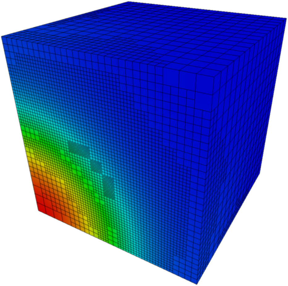
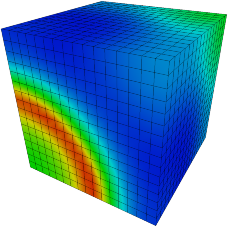
Figure 6.1: The primal (left) and adjoint (right) PDE solutions at time 0.5 ms (block no. 1).

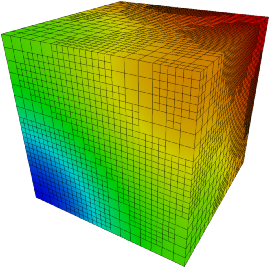
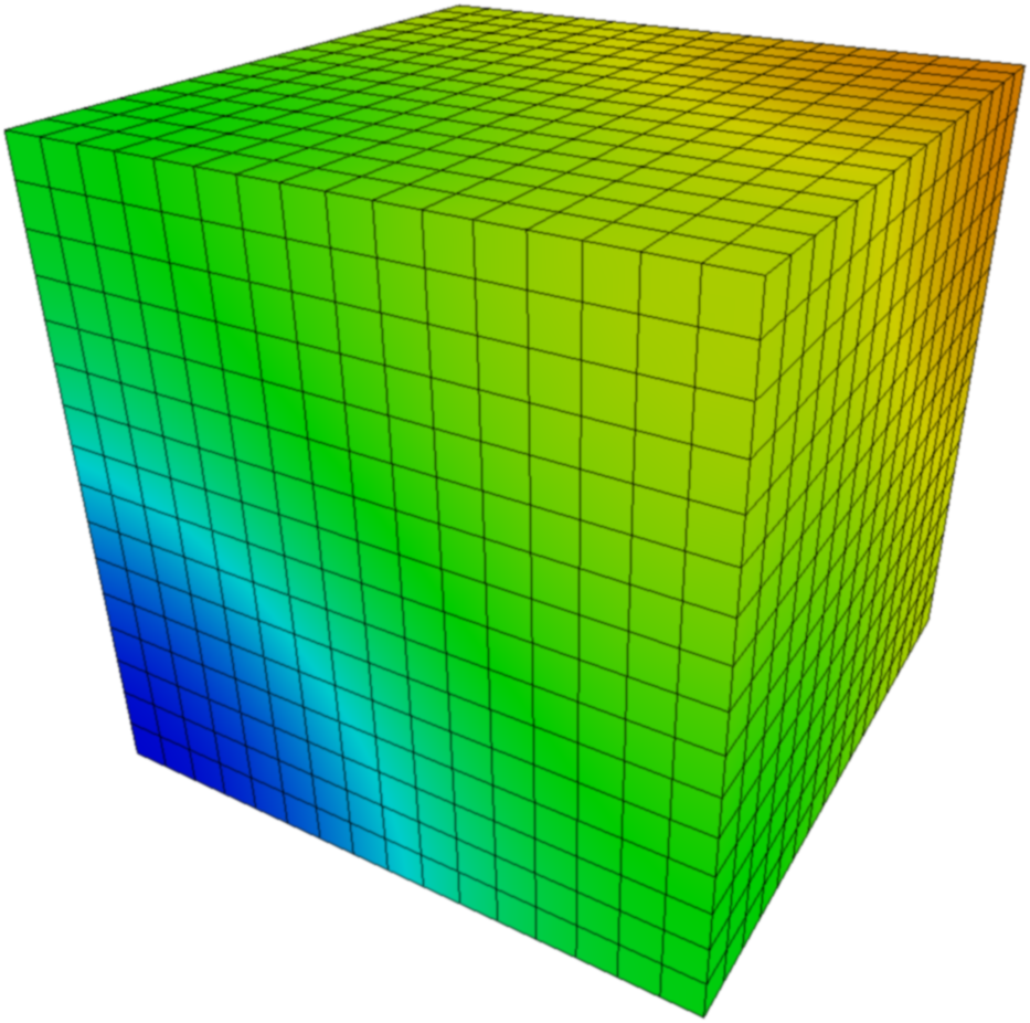
Figure 6.2: The primal (left) and adjoint (right) PDE solutions at time 200 ms (block no. 5). The range of the primal solution is $-11.76$ to $-11.70$ mV and for the adjoint solution $1.405\cdot 10^{4}$ to $1.406\cdot 10^{4}$.

The dynamics of the PDE and its adjoint are clearly visible in Fig. 6.3, which illustrates the solutions in the center of $\Omega$, i.e. at $(0.5,0.5,0.5)$. The left graph shows that there is a very steep gradient of $U$ in the first 5 ms of the simulation after which the solution then decays fairly smoothly back to its initial and resting value after about 300 ms. The adjoint solution $\Phi_{u}$ in the right plot of Fig. 6.3 has a large peak around 240 ms. This may seem surprising at first, but its explanation can be found by looking at the dynamics of the coupled ODEs in Figures 6.4, 6.5 and 6.6.

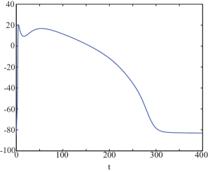
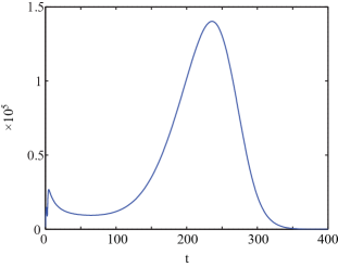
Figure 6.3: Solutions of the primal (left) and adjoint (right) PDE measured in the center of $\Omega$.

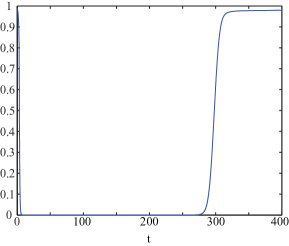
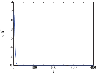
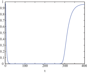
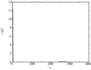
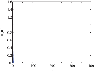
Figure 6.4: Solutions of the primal (left column) and adjoint (right column) fast ODE gating variables measured in the center of $\Omega$.

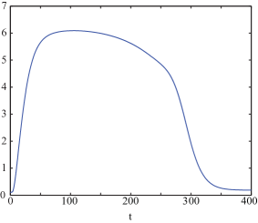
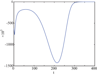
Figure 6.5: The calcium ion concentration and its adjoint measured in the center of $\Omega$.

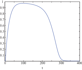
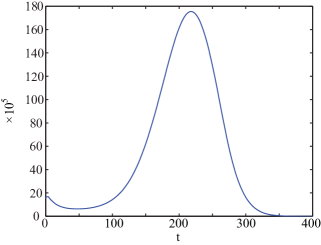
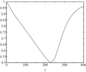
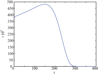
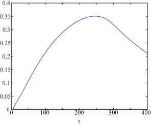
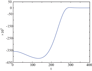
Figure 6.6: Solutions of the primal (left column) and adjoint (right column) slow ODE gating variables measured in the center of $\Omega$.

Recalling that the six of the ODE variables are gating variables and one models the calcium ion concentration, we can identify two types of gating variables by looking at Figures 6.4, 6.5 and 6.6. Three rapid gating variables in Fig. 6.4, which has a fast change in state in the beginning and then returns to its original state after about 250-350 ms – thus slightly later than the large peak of $\Phi_{u}$. Moreover, the calcium concentration in Fig. 6.5 seem to be strongly related to $\Phi_{u}$ at around 220 ms. Fig. 6.6 illustrates three slower gating variables, and similar to the calcium concentration, they are less influential for small $t$ but rather have their significance when the system goes back to its resting state.

To examine convergence properties, we evaluate the error terms after varying the number of iterations $L_{n}$ in the iterative multirate method, the spatial and temporal mesh sizes of the PDE as well as the time steps of the ODEs. These four parameters were changed uniformly to produce Figures 6.7 and 6.8. The default values in these experiments are $4096$ elements, $\Delta t=\Delta s=0.1$, $L_{n}=1$, $\mathcal{N}_{\omega}=10000$ and $T=20$. As can be seen the errors in the various terms of (4.29) decrease as expected. The main observation is that the splitting error Term $V$ dominates the total error, but can be controlled by increasing $L_{n}$, cf. Fig. 6.8. In Fig. 6.9 we show the effect of varying the number of Voronoi cells, $\mathcal{N}_{\omega}$, which also show expected behavior.

      

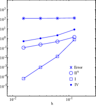
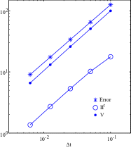
Figure 6.7: Left: Error and selected contributions as the spatial mesh size varies. Right: Error and selected contributions as the PDE time step varies.

      

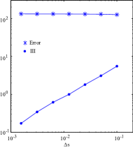
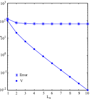
Figure 6.8: Left: Error and selected contributions as the ODE time step varies. Right: Error and selected contribution as the number of iterations $L_{n}$ in the multirate iterative scheme varies.

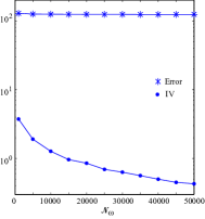
Figure 6.9: Error and selected contribution as the number of Voronoi cells $\mathcal{N}_{\omega}$ varies.

The large dynamics in the system are naturally manifested in the number of blocks, and the spatial and temporal discretizations on these blocks. With the given tolerances and parameter values, $8$ blocks are obtained and basic statistics about these blocks can be found in Table 6.1. As can be seen, the sizes of the first four blocks are limited by the xMAX criteria, with predicted number of elements being $77309$, $79829$, $94074$ and $87403$. Recalling that $\text{xMAX}=75000$, we thus obtain significantly more elements. This can be understood by looking at the block creation procedure in detail. For example, considering block 3, the predicted number of elements for the first interval $(2.3,2.4]$ was $48987$. Since this is less than xMAX, the procedure considers also the next interval $(2.4,2.5]$. The predicted number of elements for the total interval $(2.3,2.5]$ results in $71870$ elements. This is also less than xMAX, albeit close. The fact that this prediction is close to xMAX and knowing that the dynamics of the problem is rapid could suggest that the block should be ended. In the implementation here, the xMAX criterion is a strict inequality and the interval $(2.5,2.6]$ is considered. This results in a prediction of $94074$ elements to guarantee error control. The true number of elements obtained are slightly larger, although less than $1$ %, due to the constraint of having at most one hanging node per element edge.

The blocks 5, 6, 7 and 8 have the same spatial discretization with $45718$ elements. Recall that the reason for the spatial meshes not being coarsened is due to the parameter $\theta$ (5.6). As can be seen in Table 6.1, blocks 5, 6 and 7 are limited in time by the $\text{tMAX}=1000$ criteria. Finally we note that the variation in time is great: the time step size for the PDE and the ODEs are in the range of $10^{-3}$ to $1$ ms and $10^{-4}$ to $1$ ms respectively. Fig. 6.10 illustrates the various time steps over time for the PDE.

Table 6.1: Date on blocks: $b$ is the block number, $T_{b}$ is the end time in ms and $\lvert I_{b}\rvert$ is the number of time intervals in block number $b$. $\Delta t$ is the PDE time step. $M_{n}$ is the number of ODE time subintervals with $\max$ and ${\operatorname{mean}}$ values. $N_{x}$ is the number of elements that are predicted and actually used.

$b$	$T_{b}$ (ms)	$\lvert I_{b}\rvert$	$\Delta t\times 10^{-3}$ ($\mu$s)			$M_{n}$		$N_{x}$
			$\min$	$\max$	${\operatorname{mean}}$	$\max$	${\operatorname{mean}}$	predicted	used
1	1.9	352	2.27	25.0	5.41	8	2.02	77309	77554
2	2.3	182	1.63	3.58	2.21	6	2.07	79829	79899
3	2.6	173	1.61	1.93	1.74	5	2.13	94074	94158
4	2.8	120	1.51	1.89	1.68	6	2.18	87403	87508
5	159.5	1000	0.78	1000	157	6	2.04	45718	45935
6	266.4	1000	28.0	1000	107	2	2	45718	45935
7	293.7	1000	22.0	56.0	27.4	2	2	45718	45935
8	400	222	55.0	1000	481	2	2	45718	45935

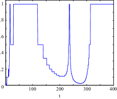
Figure 6.10: The time steps of the PDE.

7 Conclusion

We consider a problem of a macroscale parabolic PDE which is coupled to a set of microscale ODEs. We introduce an intermediate scale to couple information between the scales, and use projections to transfer information to the intermediate scale. We use a Monte Carlo method to deal with the very high dimension of the system of ODEs. We also allow the ODEs to be solved on a much finer scale than the PDE. We derive an adjoint-based a posteriori estimate that accounts for all of the key discretization components, and use the estimate to derive indicators of element contributions to the error both in space and time for the PDE and in time for the ODEs. The estimates take into account errors in the data passed between the PDE and the ODEs, as well as the fact that the ODEs are modeled on a much smaller scale than that of the PDE. The indicators are used to guide an algorithm for adaptive error control.

Finally, we test the adaptive algorithm on a realistic problem.

Future work could consider parallel blockwise adaptivity. Since the ODEs in this model do not interact inbetween spatial elements, this set of ODEs constitute an embarrassingly parallel problem and can simply be parallelized using a graphical processing unit, GPU. Developing adaptive algorithms designed for modern computer technologies with several memory hierarchies such as a GPU are indeed interesting, and the blockwise adaptivity could be one method for limiting the number of data transfers between hierarchies.

References

- [1] L. Tung, A bi-domain model for describing ischemic myocardial d-c potentials., Ph.D. thesis, Massachusetts Institute of Technology (1978).
- [2] J. Sundnes, G. T. Lines, X. Cai, B. F. Nielsen, K.-A. Mardal, A. Tveito, Computing the Electrial Activity in the Heart, Springer-Verlag, 2006.
- [3] P. Colli Franzone, P. Deuflhard, B. Erdmann, J. Lang and L. F. Pavarino, Adaptivity in space and time for reaction-diffusion systems in electrocardiology, SIAM J. Sci. Comput. 28 (2006) 942–962.
- [4] D. Noble, Modeling the heart - from genes to cells to the whole organ, Science (2002) 1678–1682.
- [5] D. Estep, Error estimation for multiscale operator decomposition for multiphysics problems, Oxford University Press, 2010, Ch. 11, Bridging the Scales in Science and Engineering, Editor: Jacob Fish.
- [6] K. Eriksson, D. Estep, P. Hansbo, C. Johnson, Introduction to adaptive methods for differential equations, Acta Numerica 4 (1995) 105–158.
- [7] K. Eriksson, D. Estep, P. Hansbo, C. Johnson, Computational Differential Equations, Cambridge University Press, New York, 1996.
- [8] D. Estep, M. G. Larson, R. D. Williams, Estimating the error of numerical solutions of systems of reaction-diffusion equations, Memoirs A.M.S. 146 (2000) 1–109.
- [9] W. Bangerth, R. Rannacher, Adaptive Finite Element Methods for Differential Equations, Birkhauser Verlag, 2003.
- [10] M. B. Giles, E. Süli, Adjoint methods for pdes: a posteriori error analysis and postprocessing by duality, Acta Numerica 11.
- [11] D. Estep, V. Ginting, D. Ropp, J. N. Shadid, S. Tavener, An a posteriori-a priori analysis of multiscale operator splitting, SIAM J. Numer. Anal. 46 (2008) 1116–1146.
- [12] V. Carey, D. Estep, S. Tavener, A posteriori analysis and adaptive error control for multiscale operator decomposition solution of elliptic systems i: Triangular systems, SIAM J. Numer. Anal. 47 (2009) 740–761.
- [13] A. Logg, Multi-Adaptive Galerkin Methods for ODEs I, SIAM J. Sci. Comput. 24 (2002) 1879–1902.
- [14] D. Estep, V. Ginting, S. Tavener, A posteriori analysis of multirate numerical method for ordinary differential equations,, Comput. Meth. Appl. Mech. Engin. 223 (2012) 10–27.
- [15] D. Estep, V. Ginting, J. Hameed, S. Tavener, A posteriori analysis of an iterative multi-discretization method for reaction–diffusion systems, Computer Methods in Applied Mechanics and Engineering 267 (0) (2013) 1 – 22.
- [16] V. Carey, D. Estep, S. Tavener, A posteriori analysis and adaptive error control for operator decomposition solution of coupled semilinear elliptic systems, Inter. J. Numer. Meth. Engin. 94 (2013) 826–849.
- [17] V. Carey, D. Estep, A. Johansson, M. Larson, S. Tavener, Blockwise adaptivity for time dependent problems based on coarse scale adjoint solutions, SIAM Journal on Scientific Computing 32 (4) (2010) 2121–2145.
- [18] F. Aurenhammer, Voronoi diagrams – a survey of a fundamental geometric data structure, ACM Comput. Surv. 23.
- [19] M. Ainsworth, B. Senior, Aspects of an adaptive hp-finite element method: Adaptive strategy, conforming approximation and efficient solvers, Computer Methods in Applied Mechanics and Engineering 150 (1997) 65 – 87.
- [20] S. F. Frisken, R. N. Perry, Simple and efficient traversal methods for quadtrees and octrees, Graphics tools: The JGT editors’ choice.
- [21] C. H. Rycroft, Voro++: A three-dimensional Voronoi cell library in C++, Chaos: An Interdisciplinary Journal of Nonlinear Science 19.
-
[22]
S. Balay, et al., PETSc Web page,
http://www.mcs.anl.gov/petsc (2014).
URL http://www.mcs.anl.gov/petsc - [23] G. W. Beeler, H. Reuter, Reconstruction of the action potential of ventricular myocardial fibres, J Physiol. 268 (1) (1977) 177–210.
- [24] A. L. Hodgkin, A. F. Huxley, A Quantitative Description of Membrane Current and its Application to Conduction and Excitation in Nerve, Journal of Physiology 4 (1952) 500–544.