A new encoding of coalescent processes.
Applications to the additive and multiplicative cases.

Abstract

We revisit the discrete additive and multiplicative coalescents, starting with $n$ particles with unit mass. These cases are known to be related to some “combinatorial coalescent processes”: a time reversal of a fragmentation of Cayley trees or a parking scheme in the additive case, and the random graph process $(G(n,p))_{p}$ in the multiplicative case. Time being fixed, encoding these combinatorial objects in real-valued processes indexed by the line is the key to describing the asymptotic behaviour of the masses as $n\to+\infty$.

We propose to use the Prim order on the vertices instead of the classical breadth-first (or depth-first) traversal to encode the combinatorial coalescent processes. In the additive case, this yields interesting connections between the different representations of the process. In the multiplicative case, it allows one to answer to a stronger version of an open question of Aldous [Ann. Probab., vol. 25, pp. 812–854, 1997]: we prove that not only the sequence of (rescaled) masses, seen as a process indexed by the time $\lambda$, converges in distribution to the reordered sequence of lengths of the excursions above the current minimum of a Brownian motion with parabolic drift $(B_{t}+\lambda t-t^{2}/2,t\geq 0)$, but we also construct a version of the standard augmented multiplicative coalescent of Bhamidi, Budhiraja and Wang [Probab. Theory Rel., to appear] using an additional Poisson point process.

Mathematics Subject Classification (2000): 60C05, 60K35, 60J25, 60F05, 68R05
Keywords: multiplicative coalescent, additive coalescent, random graph, Cayley tree, invasion percolation, Prim’s algorithm.

1 Introduction

Consider a family of weighted particles (carrying a mass, or a size) which (informally) merge according to the following rule: given some non-negative symmetric collision kernel $K$, each pair of particles with masses $x$ and $y$ collides at rate $K(x,y)$, upon which they coalesce to form a single new particle of mass $x+y$ (later on, this is sometimes referred to as a cluster). A mean-field model is provided by Smoluchowski’s equations [30], which consist in an infinite system of ordinary differential equations characterising the joint evolution of the densities of particles of each mass as time goes. The systems are only solved in some special cases, among which one may cite the cases when the kernel is either additive, $K(x,y)=x+y$, or multiplicative, $K(x,y)=xy$ ([5, 8], see [16] for more recent and general results).

Arguably, one of the objectives in the field of coalescent processes is to tend towards models of physical systems that would be more realistic “at the particles level”, even if many of the features of real systems are still ignored, starting with the positions in space and energies of the particles. For an overview of the literature on these issues, and of the relation between coalescence processes and Smoluchowski’s equations, we refer the interested reader to Aldous’ survey [5], Pitman [28], or Bertoin [8].

When the number of particles is finite, it is rather easy to define rigorously a Markov process having the dynamics discussed in the first paragraph above. One possible construction is the so-called Marcus–Lushnikov [26, 24] coalescence process. Informally, consider the masses as vertices of a complete graph, and equip the edges between vertices $i$ and $j$ with random exponential clocks with parameter $K(x_{i},x_{j})$. When the clock between $i$ and $j$ rings, replace the masses $x_{i}$ and $x_{j}$ on the nodes $i$ and $j$ by $x_{i}+x_{j}$ and $0$, respectively, and update the parameters of the clocks involving $i$ and $j$ so that the rates remain given by the kernel. When the number of masses is infinite, the definition of coalescence processes is much more involved. These issues are discussed and solved for important classes of kernels in Evans & Pitman [15] and in Fournier & Löcherbach [17] (see also references therein, and [5]).

In this paper we focus on the additive and multiplicative kernels. Together with Kingman’s coalescent (for which $K(x,y)=1$), the associated coalescence processes are somehow the simplest, but also some of the most important. This is mostly because of their manifestations in fundamental discrete models that we will call hereafter combinatorial coalescence processes. These “incarnations” are forest-like or graph-like structures modelling the coalescence at a finer level which (partially) keep track of the history of the coalescing events [15, 4, 3, 8, 7, 13, 27, 28, 9].

Invasion percolation and linear representations. Most importantly for us, both the additive and the multiplicative coalescents started with unit-mass particles admit a graphical representation as (a time change of) the process of level sets of some weighted graph: there exists some (random) graph and random weights such that at each time $t$, the clusters are the connected components of the graph consisting of all edges of weight at most $t$. We call such processes percolation systems. For the multiplicative coalescent, the graph is simply the complete graph weighted by independent and identically distributed (i.i.d.) random variables uniform on $[0,1]$; the additive case arises when taking the graph as a uniformly random labelled tree, and the weights to be i.i.d. uniform that are also independent of the tree. The idea underlying our work relies on invasion percolation [12, 23] or equivalently on Prim’s algorithm [19, 29] to obtain an order on the vertices of such percolation systems, which we refer to as the Prim order and that is consistent with the coalescent in a sense that we make clear immediately. Given a connected graph whose edges are marked with non-negative and distinct weights, and a starting node, say $v_{1}$, Prim’s algorithm grows a connected component from $v_{1}$, each time adding the endpoint of the lightest edge leaving the current component (see Section 4). Prim order “linearises” the coalescent in a consistent way: at all times, the clusters are intervals of the Prim order, so that, in particular the clusters that coalesce are always “adjacent” (Proposition 11). Furthermore, it is remarkable that this definition of an alternate (random) order makes the consistence in time transparent and exact at the combinatorial level. We believe that that this new point of view should lead to further advances in the study of coalescence processes.

Aside from this new unifying idea which is interesting on its own, our main contributions about the multiplicative and additive coalescent are the following:

Multiplicative coalescent. We prove that the representation of the asymptotic cluster masses in terms of the excursion lengths of a functional of a Brownian motion with parabolic drift that Aldous [3] proved valid for some fixed time (convergence of a marginal) can be extended to a convergence as a time-indexed process (convergence as a random function). This answers in particular Question 6.5.3 p. 851 of Aldous [3]. The combinatorial coalescence process of interest is the percolation process on the complete graph, which is nothing else than the classical (Erdős–Rényi) random graph process $(G(n,p),p\in[0,1])$ (see Section 3.1) seen around $p=1/n+O(1/n^{-4/3})$. Furthermore, we also construct a version of the standard augmented multiplicative coalescent of Bhamidi, Budhiraja, and Wang [10] using only a Brownian motion and a Poisson point process. This process has been constructed as the scaling limit of the sequence of cluster sizes and excesses of critical random graphs, see Section 2 for more details.

Additive coalescent. Here the central combinatorial model is the percolation process on a uniformly random labelled tree, hereafter referred to as ${\sf CP}_{+}^{\textsc{ap}}$ which has initially been built using random forests. The construction due to Pitman [27] (see also references there for a complete and long history of the problem) leads to a continuous representation of the standard additive coalescent in terms of the time reversal of a fragmentation process (the logging process) of the Brownian continuum random tree (see Aldous and Pitman [4]). We introduce a slight modification of the parking model, that we refer to as ${\sf CP}_{+}^{\textsc{cl}}$, constructed by Chassaing and Louchard [13] as an approximation of the additive coalescence process. Our model ${\sf CP}_{+}$ is equivalent to ${\sf CP}_{+}^{\textsc{cl}}$ up to a random time change. Again ${\sf CP}_{+}$ is a one-dimensional model in which only consecutive blocks merge as time evolves. Our contribution here is to unify these results by showing that the model ${\sf CP}_{+}$ can be used to encode ${\sf CP}_{+}^{\textsc{ap}}$. Similarly to what is done in [13], the blocks (resp. limiting blocks) have a representation in terms of the excursion lengths of some associated random walks (resp. functional of the normalised Brownian excursion) indexed by a two-dimensional domain (space and time). In this case, the limiting process is the standard additive coalescent and its construction using a Brownian excursion was already known ([7, 13]).

2 Main results about additive and multiplicative coalescents

We present here the consequences of our work in terms of coalescence processes. Write $\ell^{p}_{\downarrow}$ for the set of non increasing sequences of non-negative real numbers belonging to $\ell^{p}$ equipped with the standard $\ell^{p}$ norm, $\|x\|_{p}=\left(\sum_{i}|x_{i}|^{p}\right)^{1/p}$. As explained in Evans and Pitman [15], $\ell^{p}_{\downarrow}$ is a convenient space to describe coalescence processes. Consider an element ${\bf x}=(x_{i},i\geq 1)$ of this space as a configuration, $x_{i}$ being the mass of particle $i$. When two particles with masses $x_{i}$ and $x_{j}$ merge, their masses are removed from ${\bf x}$, and replaced by one mass $x_{i}+x_{j}$ and another one with mass zero, inserted at the positions that ensure that the resulting configuration remains a non-increasing sequence of masses.

The Marcus–Lushnikov ([26, 24], see also [3]) definition of the finite-mass additive (resp. multiplicative) coalescent can be extended to sequences of masses in $\ell^{1}$ (resp. $\ell^{2}$) (see [4] and [3]). More precisely, Aldous [3, Proposition 5] (resp. Evans & Pitman [15, Theorem 2]) proved that there exists a Feller Markov process taking values in $\ell^{2}_{\downarrow}$ (resp. $\ell^{1}_{\downarrow}$) which has the dynamics of the multiplicative (resp. additive) coalescent.

Let $X^{n}$ be the additive coalescent process started at time $0$ in the state $(1/n,\dots,1/n,0,0,\dots)\in\ell^{1}_{\downarrow}$, a configuration with $n$ particles each having mass $1/n$. Evans & Pitman [15] (see also Aldous & Pitman [4, Proposition 2]), proved that

$$\Big{(}X^{n}\Big{(}t+\frac{1}{2}\log n\Big{)}\Big{)}_{-\infty<t<+\infty}\xrightarrow[n]{(d)}\left(X^{\infty}_{+}(t)\right)_{-\infty<t<+\infty}$$

for the Skorokhod topology on $\mathbb{D}((-\infty,+\infty),\ell^{1}_{\downarrow})$, the space of cadlag functions from $(-\infty,+\infty)$ taking values in $\ell^{1}_{\downarrow}$, where the limiting process is also an additive coalescent, called the standard additive coalescent (see also Section 3.2.1).

In the multiplicative case, Aldous [3, Proposition 4] states that starting with a configuration with $n$ particles of mass $n^{-2/3}$, when the parameters of the exponential clocks between clusters are the product of their masses, then the sorted sequence of cluster sizes present at time $n^{1/3}+t$ (for a fixed $t$) converges in distribution in $\ell^{2}_{\downarrow}$ to some sequence $\boldsymbol{\gamma}^{\times}(t)$ (described below). In Corollary 24, he shows that there exists a Markov process, called the standard multiplicative coalescent, whose distribution at time $t$ coincides with $\boldsymbol{\gamma}^{\times}(t)$, and whose evolution is that of the multiplicative (Marcus–Lushnikov) coalescent. Nevertheless, with the construction he proposes, he is not able to prove that, as a process, $\boldsymbol{\gamma}^{\times}$ is the standard multiplicative coalescent.

The marginals of these standard coalescents both possess a representation using Brownian-like processes. Let ${\sf e}$ be a normalised Brownian excursion (with unit length) and let ${\sf B}$ be a standard Brownian motion. Define

$${\sf y}^{(\lambda)}_{\times}(x) ={\sf B}(x)+\lambda x-x^{2}/2, x\geq 0,\lambda\in`R$$

$${\sf y}^{(\lambda)}_{+}(x) ={\sf e}(x)-\lambda x, x\in[0,1],\lambda>0$$

and consider the operator $\Psi$ on the set of continuous functions $f:\Lambda\to`R$ defined by

$$\Psi f(x)=f(x)-\min\{f(y)~{}:y\leq x\},~{}~{}~{}~{}~{}x\in\Lambda$$ (1)

where $\Lambda=[0,+\infty)$ or $\Lambda=[0,1]$ is the domain of $f$. An interval $I=[a,b]$ is said to be an excursion of $f$ (resp. of $f$ above its minimum) if $f(a)=f(b)=0$ and $b=\inf\{t>a,f(t)=0\}$ (resp. if $f(a)=f(b)=\min\{f(t)~{}:t\leq b\}$). An important property of $\Psi$ is the following immediate lemma, which is illustrated in Fig. 1.

Lemma 1.

If $f(0)=0$ and $g=\Psi f$, then $I=[a,b]$ is an excursion of $f$ above its minimum if and only if $I$ is an excursion of $g$ above 0. As a consequence, when these are well-defined, the multiset of the $k$ largest excursion sizes of $f$ above its minimum and of $g$ above 0 coincide.

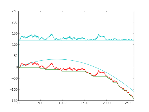
Figure 1: A simulation of the processes ${\sf y}_{\times}^{(\lambda),n}$ (bottom) and $\Psi{\sf y}_{\times}^{(\lambda),n}$ (top), with the green line materializing the infimum process. Observe the correspondance between the excursions above 0 in the top picture with that above the minimum in the bottom one.

Let $\boldsymbol{\gamma}^{+}(\lambda):=(\gamma^{+}_{i}(\lambda))_{i\geq 1}$ and $\boldsymbol{\gamma}^{\times}(\lambda):=(\gamma^{+}_{i}(\lambda))_{i\geq 1}$ be the sequence of lengths of the excursions of $\Psi{\sf y}_{+}^{(\lambda)}$ and of $\Psi{\sf y}_{\times}^{(\lambda)}$, respectively, sorted in decreasing order. Clearly, for any $\lambda\geq 0$, $\gamma^{+}(\lambda)\in\ell_{\downarrow}^{1}$ and, by Aldous [3, Lemma 25], for any $\lambda\in`R$, $\boldsymbol{\gamma}^{\times}(\lambda)\in\ell_{\downarrow}^{2}$. Then, it is known that for any integer $k$ and real numbers $\lambda_{1}<\lambda_{2}<\dots<\lambda_{k}$ the vectors

$$(\boldsymbol{\gamma}^{+}(-\ln(\lambda_{1})),\dots,\boldsymbol{\gamma}^{+}(-\ln(\lambda_{k})))\quad\text{and}\quad(\boldsymbol{\gamma}^{\times}(\lambda_{1}),\dots,\boldsymbol{\gamma}^{\times}(\lambda_{k}))$$

are distributed as the marginals at times $(\lambda_{1},\dots,\lambda_{k})$ of the standard additive and multiplicative coalescent, respectively (for the additive case, see Bertoin [7] and Chassaing–Louchard [13]; for the multiplicative case, see Aldous [3] for the marginal convergence, and Bhamidi et al. [10] for the finite-dimensional distributions).

Bertoin [7] also proved that the process $(\boldsymbol{\gamma}^{+}(-\ln(\lambda)))_{\lambda\geq 0}$ is a version of the standard additive coalescent. A similar statement has been announced by Armendariz [6] for $(\boldsymbol{\gamma}^{\times}(\lambda))_{\lambda\in\mathbb{R}}$, but has never been published. Both [7] and [6] argue directly in the continuum (Chassaing and Louchard [13, Theorem 4.2] proceeded from a parking scheme, see Section 3.2.2, and proved only convergence of marginals). The main purpose of this paper is to give a simple and unified proof of these results based on discrete versions of the coalescents. The objects involved are, as we said earlier, a parking scheme in the additive case and the random graph process $(G(n,p))_{p}$ in the multiplicative one. More precisely, our approach relies on encodings of these objects using discrete analogues of ${\sf y}_{+}^{(\lambda)}$ and ${\sf y}_{\times}^{(\lambda)}$, denoted by ${\sf y}_{+}^{(\lambda),n}$ and ${\sf y}_{\times}^{(\lambda),n}$. The associated processes

$$\boldsymbol{\gamma}^{+}(n,\lambda):=(\gamma^{+}_{i}(n,\lambda))_{i\geq 1}\qquad\text{and}\qquad\boldsymbol{\gamma}^{\times}(n,\lambda):=(\gamma^{+}_{i}(n,\lambda))_{i\geq 1}$$

will be seen (and this is standard) to coincide with lengths of their excursions above their respective minima (up to some details, see Note 6).

Using the Prim order alluded above, the strength of these encodings will appear to be that the lengths of the excursions of $\Psi{\sf y}_{+}^{(\lambda),n}$ (resp. $\Psi{\sf y}_{+}^{(\lambda),n}$) correspond, up to a time change and a normalisation, to the cluster sizes in an additive (resp. multiplicative) coalescent process, as a time-indexed process ($\lambda$ plays the role of time). In particular, as $\lambda$ grows, only successive excursions of $\Psi{\sf y}^{(\lambda),n}$ merge, which translates the fact that the Prim order linearises the additive and multiplicative processes, in the sense that it makes them consistent with a linear order.

Again, the construction in the additive case is close to that of Chassaing–Louchard [13] where the same property holds. As developed in Section 3.2.4, the novelty here is that our combinatorial additive coalescent corresponds to the linearisation of the time reversal of a fragmentation of a uniform Cayley tree defined by Pitman (see Section 3.2.1). We show that in a suitable space

$${\sf y}^{(\lambda),n}_{+}(x)\xrightarrow[n]{(d)}{\sf y}^{(\lambda)}_{+}(x)$$

as a process indexed by $(\lambda,x)$ (see Theorem 8).

The linearisation in the multiplicative case is new and allows us to prove the convergence of ${\sf y}^{(\lambda),n}_{\times}(x)$ to ${\sf y}^{(\lambda)}_{\times}(x)$ as a process indexed by $(\lambda,x)$ (see Theorem 5).

Using the properties of $\Psi$ and of the operator “extraction of excursion sizes”, we prove:

Theorem 2.

We have

$$(\boldsymbol{\gamma}^{+,n}(\lambda):\lambda\geq 0)\xrightarrow[n]{(d)}(\boldsymbol{\gamma}^{+}(\lambda):\lambda\geq 0)$$ (2)

and

$$(\boldsymbol{\gamma}^{\times,n}(\lambda):\lambda\in\mathbb{R})\xrightarrow[n]{(d)}(\boldsymbol{\gamma}^{\times}(\lambda):\lambda\in\mathbb{R})$$

in the sense of Skorokhod convergence on $\mathbb{D}(\mathbb{R},\ell^{1}_{\downarrow})$ and $\mathbb{D}(\mathbb{R},\ell_{\downarrow}^{2})$, respectively.

A a corollary, using a correspondence with coalescence (which in the additive case amounts to clarifying the time change) we establish that

Corollary 3.

The processes $(\boldsymbol{\gamma}^{+}(e^{-t}))_{t\in\mathbb{R}}\mathrel{\mathop{\kern 0.0pt=}\limits^{(d)}}(X^{\infty}_{+}(t))_{t\in\mathbb{R}}$ and $(\boldsymbol{\gamma}^{\times}(\lambda))_{\lambda\in\mathbb{R}}$ are versions of the additive and multiplicative coalescent, respectively.

There, the statement means that $(\boldsymbol{\gamma}^{+}(e^{-t}))_{t\in\mathbb{R}}$ is a Markov process taking values in $\ell^{1}_{\downarrow}$ such that for every $t$, $\boldsymbol{\gamma}^{+}(e^{-t})$ is distributed as follows [4]. Consider a Brownian continuum random tree ${\cal T}$ [2] with mass measure $\mu$ and length measure $l$ on its skeleton $\operatorname{Sk}({\cal T})$. Consider a Poisson point process $\mathcal{P}$ of intensity measure $l\otimes ds$ on $\operatorname{Sk}({\cal T})\times[0,\infty)$. At time $s$, splits ${\cal T}$ at the marks $u$ such that $(u,t)\in\mathcal{P}$ and $t\leq s$, and denote by ${\bf F}(s):=(\mathcal{F}_{1}(s),\mathcal{F}_{2}(s),\dots)$ the sequence of the $\mu$-masses of the connected components (subtrees) obtained, sorted in decreasing order. Then, for every $s\in\mathbb{R}$, we have ${\bf F}(s)\in\ell^{1}_{\downarrow}$ and $\|{\bf F}(s)\|_{1}=1$. With this setting, $(\boldsymbol{\gamma}^{+}(s))_{s\in\mathbb{R}}$ and $({\bf F}(s))_{s\in\mathbb{R}}$ have the same distribution, a result which is originally due to Bertoin [7].

In the multiplicative case, this means that $(\boldsymbol{\gamma}^{\times}(\lambda))_{\lambda\in\mathbb{R}}$ is a Markov coalescent process taking values in $\ell^{2}_{\downarrow}$ such that for every $\lambda\in\mathbb{R}$, the vector $\boldsymbol{\gamma}^{\times}(\lambda)$ is distributed as the limit rescaled component sizes of the random graph $G(n,p_{\lambda}(n))$ for

$$p_{\lambda}(n)=\frac{1}{n}+\frac{\lambda}{n^{4/3}}.$$ (3)

The existence of such a process, the standard multiplicative coalescent, has been proved by Aldous [3, Corollary 24] by resorting to Kolmogorov’s extension theorem. Here, we provide an explicit construction of the process from a single Brownian motion. The fact that the coalescing rates are multiplicative is a direct consequence of weak convergence used for the construction. The proofs of Theorem 2 and of Corollary 3 are postponed until Section 7.

In the multiplicative case, we also construct a version of the standard augmented multiplicative coalescent of Bhamidi et al. [10] as a “decorated” process of $\boldsymbol{\gamma}^{\times}$. For a connected graph, let the excess be the minimum number of edges that one must remove in order to obtain a tree. Then, the augmented multiplicative coalescent is the scaling limit of the sizes and excesses of the connected components of $G(n,p_{\lambda}(n))$, that is of $(\boldsymbol{\gamma}^{\times,n}(\lambda),{\bf s}^{n}(\lambda))$ where ${\bf s}^{n}(\lambda)=(s_{i}^{n},i\geq 1)$ and $s_{i}^{n}$ is the excess of the $i$th largest connected component of $G(n,p_{\lambda}(n))$. The zero-set $\{x\geq 0:\Psi{\sf y}_{\times}^{(\lambda)}(x)=0\}$ separates the half-line $\mathbb{R}^{+}$ into countably many open intervals $(I_{i}(\lambda))_{i\geq 1}$ whose lengths are precisely the components of the vector $\boldsymbol{\gamma}^{\times}(\lambda)$. Let $\Xi$ be a Poisson point process with unit rate on $\mathbb{R}^{+}\times\mathbb{R}^{+}$. Then, for each $\lambda\in\mathbb{R}$ and for each $i\geq 1$, let $s_{i}(\lambda)$ denote the number of points of $\Xi$ falling under the graph of $\Psi y_{\times}^{(\lambda)}$ on the interval $I_{i}(\lambda)$, the interval corresponding to the $i$-th longest excursion of $\Psi y_{\times}^{(\lambda)}$:

$$s_{i}(\lambda):=\#\big{\{}(x,w)\in\Xi:x\in I_{i}(\lambda),w\leq\Psi{\sf y}_{\times}^{(\lambda)}(x)\big{\}}.$$

Then write ${\bf s}(\lambda)=(s_{i}(\lambda))_{i\geq 1}$. The state space of interest is now $\mathbb{U}_{\downarrow}$ defined by

$$\mathbb{U}_{\downarrow}:=\bigg{\{}({\bf x},{\bf s})\in\ell^{2}_{\downarrow}\times`N^{\infty}:\sum_{i\geq 1}x_{i}s_{i}<\infty\text{~{}and~{}}s_{i}=0\text{~{}whenever~{}}x_{i}=0\bigg{\}}$$

endowed with the metric

$$\operatorname{d}_{\mathbb{U}}(({\bf x},{\bf s}),({\bf x}^{\prime},{\bf s}^{\prime})):=\Bigg{(}\sum_{i\geq 1}|x_{i}-x_{i}^{\prime}|^{2}\Bigg{)}^{1/2}+\sum_{i\geq 1}|x_{i}s_{i}-x_{i}^{\prime}s_{i}^{\prime}|~{}.$$

Theorem 4.

The following convergence

$$((\boldsymbol{\gamma}^{\times,n}(\lambda),{\bf s}^{n}(\lambda)):\lambda\in\mathbb{R})\xrightarrow[n]{(d)}((\boldsymbol{\gamma}^{\times}(\lambda),{\bf s}(\lambda)):\lambda\in\mathbb{R})$$

holds in $\mathbb{D}(\mathbb{R},\mathbb{U}_{\downarrow})$. In particular, $(\boldsymbol{\gamma}^{\times}(\lambda),{\bf s}(\lambda))_{\lambda\in\mathbb{R}}$ is a version of the standard augmented multiplicative coalescent.

Observe that the metric structure of the connected components obtained in [1] from a similar representation at fixed $\lambda$ seems to be ruined by the random Prim order. A careful look at Section 4 should suffice to convince the reader that the very idea of obtaining a representation that is consistent in $\lambda$ is incompatible with tracking the internal structure of connected components.

3 Combinatorial coalescence processes and their encodings

3.1 The multiplicative case: critical random graphs

The aim of this part is to present some elements concerning the multiplicative coalescence processes, our new approach, and the main steps to the proofs of Theorem 2 and 3.

We first define the random graph process on the vertex set $[n]:=\{1,2,\dots,n\}$, for a positive integer $n$. Let $E^{n}=\{\{i,j\},i\neq j,i,j\in[n]\}$ denote the set of pairs of elements of $[n]$, the set of edges. Let $(U_{e})_{e\in E^{n}}$ be a collection of i.i.d.  uniform random variables on $[0,1]$. Let $G(n,p)$ be the graph on $[n]$ consisting of the edges $e\in E^{n}$ for which $U_{e}\leq p$. Then, $(G(n,p))_{p\in[0,1]}$ is the classical random graph process [11, 18]. It is a Markov process but not time-homogeneous (as it would have been if instead of uniform random variables we would have used exponential ones). The ordered sequence of sizes of connected components $(|C^{n}_{i}(t)|)_{i\geq 1}$ is also a Markov process, for which the initial state is $(1,1,\dots,1)$ and the components of the vector coalesce at rate which is proportional to the product of their values. Indeed, conditionally on $G(n,t)$, the next edge to be added is equally likely among the ones which are not already present, so that the probability that it joins a vertex of $C_{i}^{n}(t)$ to one of $C_{j}^{n}(t)$ is proportional to $|C_{i}^{n}(t)|\times|C_{j}^{n}(t)|$. Thus, up to a time change, the connected components in $G(n,p)$ behave as the multiplicative coalescent.

To obtain a limit theorem for these connected component sizes as a time-indexed process, our approach uses ideas from the proof by Aldous [3] of the convergence at a fixed time. He encodes the connected components into a discrete random real-valued process whose convergence implies the convergence of the sizes of the connected component. To get suitable limit theorem, the probability $p$ has to be chosen inside the critical window, that is of the form $p=p_{\lambda}(n)$, as defined in (3). The method of Aldous relies on a breadth-first traversal of the graph $G(n,p_{\lambda}(n))$. It is easily seen that, in the context of the random graph $G(n,p)$, the following “smallest-label-first” traversal has the same distribution, so that the results of Aldous [3] apply when using this modified algorithm. In the following, we call neighbourhood of a set of vertices $S$ the collection of nodes that have an edge to a node in $S$, but are not themselves in $S$.

Algorithm 1 (Standard traversal).

Traverse the vertices of a graph on $[n]$ as follows:

• Start at step $k=1$ with node $v_{1}=1$ and set $S_{1}=\{v_{1}\}$.

• At step $k+1\in\{2,\dots,n\}$, the nodes $v_{1},\dots,v_{k}$ are already known, and we have $S_{k}=\{v_{1},\dots,v_{k}\}$. Let $v_{k+1}$ be the node with smallest label among the neighbours of $S_{k}$, or if the neighbourhood of $S_{k}$ is empty, $v_{k+1}$ is the node with smallest label in $[n]\setminus S_{k}$.

Denote by $Z_{k}^{n,p_{\lambda}(n)}$ the size of the neighbourhood of $S_{k}$ and set

$$Y_{k}^{n,p_{\lambda}(n)}=Z_{k}^{n,p_{\lambda}(n)}-\#\{j\leq k,Z_{k}^{n,p_{\lambda}(n)}=0\}.$$

Then, the sizes of the connected components of $G(n,p_{\lambda}(n))$ are precisely the lengths of the intervals between the zeros of $(Z_{k}^{n,p_{\lambda}(n)},1\leq k\leq n)$ (see Section 1.3 of [3] and Lemma 12). Then define

$$y^{n,(\lambda)}(x):=\frac{Y^{n,p_{\lambda}(n)}(n^{2/3}x)}{n^{1/3}}\qquad\text{and}\qquad z^{n,(\lambda)}(x):=\frac{Z^{n,p_{\lambda}(n)}(n^{2/3}x)}{n^{1/3}}.$$

Aldous [3] proved that, for any fixed $\lambda\in\mathbb{R}$,

$$y^{n,(\lambda)}\xrightarrow[n]{(d)}{\sf y}^{(\lambda)}_{\times}\qquad\text{and}\qquad z^{n,(\lambda)}(x)\xrightarrow[n]{(d)}\Psi{\sf y}^{(\lambda)}_{\times},$$ (4)

where the convergence holds for the topology of uniform convergence on every compact.

We propose to modify a bit the traversal of the graph in Algorithm 1: instead of using the labels order to define the traversal, use the Prim order (see Section 4 for more details): that is proceed as in Algorithm 1 but replace the two instances of “the node with smallest label” by “the node with smallest Prim rank”. Observe that the Prim order on $G(n,p)$ is defined using the weights $(U_{e})_{e\in E^{n}}$ only, and thus does not depend on $p$, unlike the order given by the standard traversal used by Aldous. In the following, we add the subscript “$\times$” in the notation for the random variables defined using this modified Prim traversal, and we set

$${\sf y}^{n,(\lambda)}_{\times}(x):=\frac{Y^{n,p_{\lambda}(n)}_{\times}(n^{2/3}x)}{n^{1/3}}$$

where $Y_{\times}$ is assumed to be interpolated between integer points. Observe that in the superscript of ${\sf y}^{n,(\lambda)}$, the superscript $(\lambda)$ corresponds to the parameter $p_{\lambda}(n)$ defined in (3). In the following, the processes $\lambda\mapsto{\sf y}^{n,(\lambda)}_{\times}$ and $\lambda\mapsto{\sf y}_{\times}^{(\lambda)}$ are denoted more simply by ${\sf y}_{\times}^{n}$ and ${\sf y}_{\times}$.

Theorem 5.

The following convergence holds in $\mathbb{D}(`R,\mathbb{C}([0,\infty),`R))$,

$${\sf y}^{n}_{\times}\xrightarrow[n]{(d)}{\sf y}_{\times}$$ (5)

where $\mathbb{C}([0,\infty),`R)$ is the set of continuous functions from $[0,\infty)$ with values in $`R$.

The proof is postponed until Section 6 (and more details on the distribution of $({\sf y}^{n,(\lambda)}_{\times},\lambda\in`R)$ are given in Section 6.1).

Observe that for a fixed $\lambda$, the convergence (4) obtained by Aldous [3] implies that ${\sf y}^{n,(\lambda)}_{\times}\to{\sf y}_{\times}^{(\lambda)}$ in distribution, provided that we additionally prove that ${\sf y}^{n,(\lambda)}_{\times}$ and $y^{n,(\lambda)}$ have the same distribution, a fact that we prove in Lemma 13. We also provide a direct proof of the fixed-time convergence in Section 6.2.

Note 6.

When we are talking about interpolated discrete processes and discrete coalescence, a slight modification in the definition of excursions has to be done in order to obtain an exact correspondence between the cluster sizes and excursion sizes. For the excursion away from zero, $f(a)=f(b)=0$ and $b=\inf\{t>a:f(t)=0\}$ has to be replaced by $f(a)=f(b)=0$ and $b=\inf\{t>a+\alpha_{n}:f(t)=0\}$, where $\alpha_{n}$ is the size of a rescaled discrete step. The discrete excursions above the current minimum are defined by $a=\min\{t:f(t)=f(a)\}$, and $b=\min\{t:f(t)=f(b)\}$ with $f(b)=f(a)-\beta_{n}$, where $\beta_{n}$ is the space normalisation.

Note 7.

In order to obtain exactly the (time-homogenenous) Markovian coalescent from the random graph process, one only needs to consider a new time parameter given by $t=-\ln(1-p_{\lambda}(n))$. However, as $n\to\infty$, $-\ln(1-p_{\lambda}(n))$ and $p_{\lambda}(n)$ behave similarly (at the second order), and the study of coalescent can be done using $p_{\lambda}(n)$. We use $p_{\lambda}(n)$ in order to stay closer to the random graph model, as did Aldous [3].

3.2 Additive coalescence processes

In the three next subsections, we treat the different combinatorial coalescence processes related to the additive coalescent. The main references here are [15, 27, 4, 7, 13, 28].

3.2.1 The combinatorial coalescence process ${\sf CP}_{+}^{\textsc{ap}}$

The following discussion relies on the results by Aldous and Pitman [4], see also Pitman [27, (ii)’ p. 170]. We define a process of random forests of unrooted labelled trees $F(n,s)$, $s\geq 0$ as follows. At time $s=0$, the forest $F(n,0)$ consists of $n$ isolated trees $t_{1},\dots,t_{n}$ where $t_{i}$ is reduced to the node $i$ alone. When the number of trees is $m$, wait an exponential random variable with parameter $m-1$, then pick a pair of trees $(t_{i},t_{j})$ with $1\leq i<j\leq m$ with probability $(|t_{i}|+|t_{j}|)/(n(m-1))$, and add an edge between a uniform node in $t_{i}$ and a uniform node in $t_{j}$. Considering only the rescaled tree sizes $C^{n,s}=(C_{i}^{n,s}/n,i\geq 1)$ of the forest $F(n,s)$ (sorted and completed by an infinite sequence of 0), we have

$$(C^{n,s},s\geq 0)\mathrel{\mathop{\kern 0.0pt=}\limits^{(d)}}(X_{+}^{n}(s),s\geq 0).$$

Since any pair of trees coalesces with probability proportional to the sum of their sizes, we just need to check that the same time-scale arises in the additive coalescent. This is indeed the case, since in the latter, when $m$ particles with total unit mass are present, the first coalescence occurs after a time equal to the minimum of independent exponential random variable with parameters $K(x_{i},x_{j})$, and $\sum_{1\leq i<j\leq m}K(x_{i},x_{j})=\sum_{1\leq i<j\leq m}x_{i}+x_{j}=m-1.$ Thus in the present coalescent, if one takes $(E_{i},1\leq i\leq n-1)$ a sequence of i.i.d. exponential r.v. with parameter 1, then the number of coalescences before time $s$ is

$$M^{n}(t)=\max\bigg{\{}m\geq 0:\sum_{j=1}^{m}\frac{E_{j}}{n-j}\leq s,\bigg{\}}$$

and

$$n^{-1/2}\left(n-M^{n}\left(s+\frac{1}{2}\log n\right)\right)\to e^{-s},$$

where the convergence holds in $\mathbb{D}((-\infty,+\infty),\mathbb{R})$ (the convergence holds in fact uniformly on any compact $[-\lambda_{\star},\lambda^{\star}]$).

3.2.2 The combinatorial coalescence process ${\sf CP}_{+}^{\textsc{cl}}$

We now present quickly the model and results of Chassaing & Louchard [13]. Assume $n$ cars park on a circular parking, identified with $\mathbb{Z}/n\mathbb{Z}$, according to the following algorithm. Let $({\sf Ch}_{i},1\leq i\leq n)$ be a family of i.i.d. random variables uniform on $\mathbb{Z}/n\mathbb{Z}$. The cars park successively. When the $i-1$ first cars have already parked, car $i$ chooses place ${\sf Ch}_{i}$ and parks at the first available place in the list ${\sf Ch}_{i}$, ${\sf Ch}_{i}+1\!\!\!\mod\!n$, ${\sf Ch}_{i}+2\!\!\!\mod\!n$… Assume that $m$ cars are parked and call block a sequence of adjacent occupied places. As explained in [13, Section 8] to get a suitable relation with the additive coalescent, the correct notion of size for a block is the number of cars consecutively parked plus one. This model coincides exactly with the Marcus–Lushnikov additive process up to a random time change. When $m=m(n)=\lfloor n-\lambda\sqrt{n}\rfloor$ cars are parked, the large $n$ asymptotic evolution of the sizes of these blocks (sorted in decreasing order)

$$B^{n,\lambda}:=\frac{1}{n}(B^{n,\lambda}_{i},i\geq 0)$$

is given by the standard additive coalescent up to a time change. Here are some precisions on this time change: the time $\lfloor n-\lambda\sqrt{n}\rfloor$ coincides with the number of coalescence done. From what we said above in the additive coalescent, this occurs at a random time of order $t+(1/2)\log(n)$ for $t$ such that $\exp(-t)=\lambda$, so that for a fixed $\lambda>0$ one can prove

$$B^{n,\lambda}\xrightarrow[n]{(d)}X^{\infty}(-\ln(\lambda)).$$

More precisely, Chassaing and Louchard obtained in [13, Theorem 1.3] the convergence of the sizes of the $k$ largest blocks to that of the $k$ largest excursions of $\Psi{\sf y}_{+}^{(\lambda)}$.

3.2.3 The new combinatorial coalescence process ${\sf CP}_{+}$

Our new combinatorial coalescence process is in the mean time very close to that of Chassaing and Louchard [13] and to that of Pitman (Section 3.2.1 above). The new idea of Prim’s order makes the connection between these two models very clear, in a way that is both different from the one discussed in [13, Section 8], and similar to our approach to the multiplicative coalescent.

Although the intuition comes from the percolation model on the uniformly random labelled tree, it is convenient for the proofs to construct the process ${\sf CP}_{+}$ as follows. The connections with the parking model and the fragmentation on trees are made later on in Section 3.2.4 Consider a sequence of i.i.d. Poisson random variables $(X(i),1\leq i\leq n)$ with parameter one, and associate to this sequence the random walk

$$Y(m)=\sum_{j=1}^{m}(X(j)-1),\qquad 0\leq m\leq n.$$

Denote by $\tau_{-1}=\inf\{m~{}:~{}Y(m)=-1\}$ the hitting time of $-1$.

Further, denote by $(Y_{+}^{n}(m),0\leq m\leq n)$ the random walk $Y$ conditioned on $\tau_{-1}=n$. Denote by $(X_{+}^{n}(i),1\leq i\leq n)$ the increments of $Y_{+}^{n}$ (that is under the condition that $\tau_{-1}=n$). Now introduce an array $(U_{k}(\ell),1\leq k\leq n,1\leq\ell\leq n)$ of i.i.d. ${\sf uniform}[0,1]$ random variables and, conditionally on the family $(X^{n}_{+}(i),1\leq i\leq n)$, define the family $(X^{n,(t)}_{+}(i),0\leq t\leq 1,1\leq i\leq n)$, by

$$X_{+}^{n,(t)}(i)=\sum_{j=1}^{X_{+}^{n}(i)}1_{U_{i}(\ell)\leq t},~{}~{}\textrm{ for any }t\in[0,1],1\leq i\leq n.$$

Hence, $X^{n,(0)}_{+}(i)=0$, $X^{n,(1)}_{+}(i)=X^{n}_{+}(i)$ and for any $i$, $t\mapsto X_{+}^{n,(t)}(i)$ is non-decreasing. Define

$$Y^{n,(t)}_{+}(m)=\sum_{j=1}^{m}(X^{n,(t)}_{+}(j)-1),~{}~{}0\leq m\leq n,~{}t\in[0,1].$$

From now on, consider that $(Y^{n,(t)}_{+}(m),0\leq m\leq n)$ is a continuous process in the variable $m$, obtained by linear interpolation between integer points. Set

$${\sf y}_{+}^{n,(\lambda)}(x)=\frac{Y^{n,(1-\lambda/\sqrt{n})}_{+}(nx)}{\sqrt{n}},~{}~{}~{}x\in[0,1],\lambda\geq 0.$$

The processes $(\lambda,x)\mapsto{\sf y}^{n,(\lambda)}_{+}(x)$ and $(\lambda,x)\mapsto{\sf y}_{+}^{(\lambda)}(x)$ are denoted more simply ${\sf y}_{+}^{n}$ and ${\sf y}_{+}$ in the sequel. They are seen as random variables taking their values in $\mathbb{D}(`R^{+},\mathbb{C}([0,1],`R))$. In words, for fixed $\lambda$, ${\sf y}_{+}^{(\lambda)}$ is a r.v. in $\mathbb{C}([0,1],`R)$. Seen as a process in $\lambda$ it is right-continuous with left limits. From what we said earlier $\lambda\mapsto{\sf y}_{+}^{n,(\lambda)}$ is non-increasing in $\lambda$.

For $\lambda=0$, $Y_{+}^{n,(0)}$ is just a random walk conditioned to hit $-1$ at time $n$. By a generalisation of Donsker’s invariance principle [14], see for instance [20, 25], we have

$${\sf y}^{n,(0)}_{+}\xrightarrow[n]{(d)}{\sf y}^{(0)}_{+},$$ (6)

in $\mathbb{C}([0,1],\mathbb{R})$ equipped with the topology of uniform convergence (recall that ${\sf y}^{(0)}_{+}={\sf e}$). The proof of the next theorem is postponed until Section 5.

Theorem 8.

The following convergence holds in $\mathbb{D}(`R^{+},\mathbb{C}([0,1],`R))$,

$${\sf y}^{n}_{+}\xrightarrow[n]{(d)}{\sf y}_{+}.$$

3.2.4 Between a parking scheme and fragmentation of Cayley trees

The parking scheme point of view on ${\sf CP}_{+}$. The construction in Section 3.2.3 may be interpreted as follows in terms of a parking scheme: $X(i)$ is the number of cars whose first choice is place $i$ and that park at the first empty place to the right of $i$. The condition $\tau_{-1}=n$ amounts to saying that, in then end, the place $n$ is still empty (see [13] for more details). The random variable $X_{+}^{n,(t)}(i)$ represents the number of cars that have chosen place $i$ by time $t$. Observe that conditionally on $\tau_{-1}=n$, $\sum_{i=1}^{n}X(i)=n-1$, so that $\sum_{i=1}^{n}X^{n,(t)}_{+}(i)$ is binomial with parameters $n-1$ and $t$. In particular, this is random, unlike in [13]. Hence, at time $t=1-{\lambda}/{\sqrt{n}}$ the number of coalescences that already occurred, denoted by $N^{n,\lambda}$, is binomial$(n-1,1-\lambda/{\sqrt{n}})$ and it follows that

$$W_{n,\lambda}:=\frac{n-N^{n,\lambda}}{\sqrt{n}}\xrightarrow[n]{(d)}\lambda,$$

the convergence holding in distribution in $\mathbb{D}([0,\lambda_{\star}],\mathbb{R})$ for any $\lambda_{\star}$, since the convergence is uniform on any compact. Indeed one may check that, as a process on $[0,\lambda_{\star}]$, we have $W_{n,\lambda}=n^{-1/2}\sum_{i=1}^{n-1}1_{U^{(i)}\leq\lambda/\sqrt{n}}$ for some $(U^{(i)},i\geq 1)$ i.i.d. uniform on $[0,1]$. The process $\lambda\mapsto W_{n,\lambda}$ is non-decreasing, and its finite-dimensional distributions converge to those of the deterministic process $(\lambda,\lambda\geq 0)$ (convergence of the mean, and the variance goes to 0), and thus the convergence is almost sure (a.s.) on any compact (see [25, Appendix] if more details are needed).

The convergence of this time change between our model and the discrete coalescence process, together with the convergence of the excursion sizes (as a process in $\lambda$) are the main tool to obtain the convergence to the additive coalescent.

The percolation point of view. Consider a uniform Cayley tree with $n$ vertices (uniformly labelled tree on $[n]$), and root it at the vertex labelled $1$. For a node in $[n]$, let its out-degree be the number of its neighbours that are further from the root. Then, it is folklore that the sequence of node out-degrees $(d_{i},1\leq 1\leq n)$ where the nodes are sorted according to the breadth-first order is distributed as $(X(i),1\leq i\leq n)$ conditional to $\tau_{-1}=n$, as described above. The random walk $Y^{n,(0)}_{+}$ appears in the literature as the Łukasiewicz walk associated with a uniform Cayley tree [see, e.g., 22]. Now, equip the edges of the Cayley tree with i.i.d. uniform weights $(U_{e},e\in E)$ (independently of the tree) and keep the edges with weight smaller than $t$, discarding the others. One then obtains a forest. In this forest $F_{t}$, let $d_{i}(t)$ denote the out-degree of the node that had previously rank $i$ in the Cayley tree (so that $d_{i}(1)=d_{i}$). Then clearly,

$$(d_{i}(t),~{}1\leq i\leq n)_{t\in[0,1]}\mathrel{\mathop{\kern 0.0pt=}\limits^{(d)}}(X^{n,(t)}_{+}(i),~{}1\leq i\leq n)_{t\in[0,1]}.$$ (7)

The following proposition is a consequence of Lemma 14 (and Lemma 13):

Proposition 9.

Let $T$ be a uniform Cayley tree on $n$ vertices whose edges are (independently) equipped with i.i.d. uniform $[0,1]$ weights. Let $(u_{i},1\leq i\leq n)$ be the nodes sorted according to the Prim order (when the root node is $u_{1}=1$), and let $X^{t}(i)$ be the number of edges between $u_{i}$ and its children, that have a weight at most $t$. Then

$$(X^{t}(1),\dots,X^{t}(n))_{t\in[0,1]}\mathrel{\mathop{\kern 0.0pt=}\limits^{(d)}}(X_{+}^{n,(t)}(1),\dots,X_{+}^{n,(t)})_{t\in[0,1]}.$$

As a consequence the collection of excursion sizes of $\Psi Y^{n,(t)}_{+}$ at time $t$ evolves, up to a time change, as the additive coalescent.

It is classical that a tree (or a forest) can be encoded by a Łukasiewicz walk. This walk encodes the sequence of node degrees $(Y^{n,t}(j)=\sum_{k=1}^{j}(d_{i}^{(t)}-1))$. As a consequence, the sequence of sizes of the trees in $F_{t}$, sorted using the Prim order correspond to the sequence of excursion sizes of $\Psi Y^{n,(t)}_{+}$, and this property is true as a process indexed by $t$. This makes a connection between the results by Aldous and Pitman [4] and our representation of additive coalescent, and explains again the fact that the additive coalescent can be linearised.

4 Prim’s order and linear representations of coalescents

This part presents the main new idea underlying this work.

4.1 Prim’s algorithm and coalescents

In this section, we assume that an integer $n\geq 2$ is fixed. Let $G=([n],E)$ be any connected graph, where the edges are marked by some weights, ${\bf w}=(w_{e},e\in E)\in[0,1]^{\#E}$, some non-negative real numbers. The pair $(G,{\bf w})$ is said to be properly weighted if the weights are distinct and positive.

Prim’s algorithm (or Prim–Jarník algorithm) is an algorithm which associates with any properly weighted graph $(G,{\bf w})$ its unique minimum spanning tree, the connected subgraph of $G$ that minimises the sum of the weights of its edges. It also defines a total order $\prec$ on the set of vertices. Let us describe the nodes $u_{1},\dots,u_{n}$ satisfying $u_{1}\prec u_{2}\prec\dots\prec u_{n}$. We will use below the notation $V_{i}$ for the set $\{u_{1},\dots,u_{i}\}$.

First set $u_{1}=1$ and $V_{1}=\{u_{1}\}$. Assume that for some $1\leq i\leq n-1$, the nodes $u_{1},\dots,u_{i}$ have been defined. Consider the set of weights $\{w_{\{a,b\}}~{}|~{}a\in V_{i},b\notin V_{i}\}$ of edges between a vertex of $V_{i}$ and another outside of $V_{i}$. Since all weights are distinct, the minimum is reached at a single pair $(a^{\star},b^{\star})\in V_{i}\times\complement V_{i}$. Set $u_{i+1}=b^{\star}$. This iterative procedure completely determines the Prim order $\prec$. If one sets additionally $\pi_{i+1}=a^{\star}$, a classical result (not used in the paper) is that the minimum spanning tree is the tree on $[n]$ with set of edges $\{(\pi_{i},u_{i}):2\leq i\leq n\}$.

Definition 10.

We say that a set of nodes $\{v_{1},\dots,v_{\ell}\}$ forms a Prim interval, if $\{v_{1},\dots,v_{\ell}\}=\{u_{i},i\in\llbracket a,a+\ell-1\rrbracket\}$ for some $a$, that is if their Prim ranks are consecutive. Any Prim interval can be written as $V_{j}\setminus V_{i}$ for some pair $(i,j)$.

Given a properly weighted graph $(G,{\bf w})$, for any $t\in[0,1]$, $E_{t}({\bf w})=\{e\in E:w_{e}\leq t\}$ and $G_{t}({\bf w})=([n],E_{t})$ the graph whose edges are the edges of $E$ with weight at most $t$. The next proposition, which seems to be folklore in graph theory, is of prime importance to us. In the sequel we write $E_{t}$ and $G_{t}$ for short, the weights being clear from the context.

Proposition 11.

Let $(G,{\bf w})$ be a properly weighted graph. For any $t\in[0,1]$, all the connected components of $G_{t}$ are Prim intervals. As a consequence, the coalescence of connected components arising when $t$ increases corresponds to coalescence of consecutive Prim intervals.

Figure 2: A realisation of the weighted complete graph $G$ on $[6]=\{1,2,\dots,6\}$ where only the edges with weight at most $0.9$ are drawn. On the right, only the edges $e$ such that $w_{e}\leq 0.5$ are kept (this is $G_{0.5}$), and the $u_{i}$’s are the nodes sorted according to the Prim order. Notice that the connected components are intervals in the Prim order. In this example, $\mathcal{Z}^{0.5}(1)=\{u_{2}\},\mathcal{Z}^{0.5}(2)=\{u_{3}\},\mathcal{Z}^{0.5}(3)=\varnothing,\mathcal{Z}^{0.5}(4)=\{u_{5}\},\mathcal{Z}^{0.5}(5)=\varnothing,\mathcal{Z}^{0.5}(6)=\varnothing$.

Proof.

Only the first statement needs to be proved. The graph $G_{t}$ is non-decreasing for $t\in[0,1]$, and since by hypothesis the weights are distinct and non-zero, we have $E_{0}=\varnothing$ and $E_{1}=E$. The finite set of weights/times $\{w_{e},e\in E\}$ are the jumping times for the function $(G_{t},0\leq t\leq 1)$, and exactly $n-1$ of these dates $t_{1},\dots,t_{n-1}$ modify the number of connected components. So the result needs only be checked at these times. For $t=t_{0}=0$ the result holds. Assume that, at time $t_{k}$ for some $0\leq k\leq n-2$, all the connected components are consecutive intervals $(I_{1},\dots,I_{\ell})$ with $I_{j}=[a_{j},b_{j}]$ and $a_{j+1}=b_{j}+1$. Denote by $e$ the edge which is added at time $t_{k+1}$. By hypothesis adding it decreases the number of connected components, and so its end points lie in two distinct intervals $I_{x}=[a_{x},b_{x}]$ and $I_{y}=[a_{y},b_{y}]$ for some $x<y$. If $y=x+1$ we are done, so assume for a contradiction that $y>x+1$. The weight $w_{e}$ is smaller than all those of the missing edges at time $t_{k+1}$; in particular, it is smaller than all the weights of the edges between $\cup_{i\leq x}I_{i}$ and $I_{x+1}$. But this is impossible, since it contradicts the fact that the vertices are sorted according to the Prim order: indeed, by definition, the extremity of the lightest edge out of $\cup_{i\leq x}I_{i}$ is $a_{x+1}\in I_{x+1}$. ∎

Denote by ${\sf Neigh}^{G}(v)=\{u~{}:\{u,v\}\in E\}$ the set of neighbours of $v$ in $G$. For a set of nodes $S$ let also ${\sf Neigh}^{G}(S)=\left(\bigcup_{v\in S}{\sf Neigh}^{G}(v)\right)\setminus S$, the set of neighbours of $S$ (out of $S$). Aldous [3] study of the multiplicative coalescent relies on an exploration of the graph and an encoding of the process $i\mapsto\#{\sf Neigh}^{G}(S_{i})$, for an increasing collection of sets $(S_{i})_{1\leq i\leq n}$ that are built by a breadth-first search algorithm. The modified Algorithm 1 uses the standard order on the nodes instead of breadth-first search, but here we investigate the influence of the order on $[n]$, hereafter denoted by $<$, that is used in building the sets $(S_{i})_{1\leq i\leq n}$. The exploration is as follows.

The first visited node is the smallest one $v_{1}$ for the order $<$. Assume we have visited $S_{k}=\{v_{1},\dots,v_{k}\}$ at some time $1\leq k\leq n$. Then two cases arise:

• if ${\sf Neigh}^{G}(S_{k})\neq\varnothing$, then $v_{k+1}$ is the smallest node for $<$ in ${\sf Neigh}^{G}(S_{k})$, or

• if ${\sf Neigh}^{G}(S_{k})=\varnothing$, then $v_{k+1}$ is the smallest node for $<$ in $[n]\setminus S_{k}$.

In the exploration used by Aldous, the labels of the nodes $1,2,\dots,n$ are compared using the standard order $<$ on $\mathbb{N}$. The exploration clearly depends on the order $<$, and the notation should have reflected this fact. For example, we could have written $v_{k}(<)$ and $S_{k}(<)$ instead of $v_{k}$ and $S_{k}$. We will sometimes used further these enriched notation, and for $0\leq k\leq n+1$ we also use the more compact notation

$$Z^{g}_{<}(k)=\#{\sf Neigh}^{g}(S_{k}(<))$$

where by convention $Z^{g}_{<}(0)=Z^{g}_{<}(n+1)=0$.

The proof of the following lemma is immediate. For a graph $g=([n],E)$, denote by ${\sf CC}(g)$ the set of connected components of $g$, seen as a partition of $[n]$.

Lemma 12.

Let $g=([n],E)$ be a graph (connected or not). For any total order $<$ on the set of nodes $[n]$,

$$\#\{k\in\{0,\dots,n\}~{}:Z^{g}_{<}(k)=0\}=\#{\sf CC}(g),$$

and the successive sizes of the connected components ordered by the exploration coincide with the distances between successive zeros in the sequence $(Z^{g}_{<}(k),0\leq k\leq n+1)$.

In the following we will call Prim exploration the exploration based on the Prim order $\prec$. Unlike the standard exploration, it is defined only on properly weighted graphs $(G,{\bf w})$.

4.2 Prim traversal versus standard traversal

Take a random graph ${\bf G}=([n],E)$ whose edges are equipped with i.i.d. uniform [0,1] weights. Let us examine the similarities and the differences between the standard exploration (using the order $<$) and the Prim exploration of the random graph ${\bf G}_{t}$. By Lemma 12 the multiset of excursions lengths of $Z^{{\bf G}_{t}}_{<}$ and $Z^{{\bf G}_{t}}_{\prec}$ are the same, but in general the paths $Z^{{\bf G}_{t}}_{<}$ and $Z^{{\bf G}_{t}}_{\prec}$ do not have the same distribution. We already said that the distributions of the corresponding processes in $t$ were different (by Proposition 11), but this is also true for fixed $t$ (even if the distribution of ${\bf G}$ is invariant by random permutation of the node labels). The reason is that during the exploration, the Prim order favours the nodes with a large indegree since the order is defined using the weights of the edges. Here is an example illustrating this. Consider ${G}$ the graph with vertices $\{1,a_{1},a_{2},a_{3}\}$ and edges $(1,a_{1}),(1,a_{2}),(1,a_{3}),(a_{2},a_{3})$. Conditionally on ${\bf G}_{t}=G$, one sees that for the standard exploration, under a random labelling preserving $1$, one visits $1,a_{2},a_{3},a_{1}$ in that order with probability $1/6$. However, under the Prim exploration, it is easy to check that, among the 24 possible orderings of the weights $(w_{e},e\in E)$, six of them give this order so that the probability is $1/4$.

There are however some special cases, including when ${\bf G}$ is a uniform Cayley tree or the complete graph for which the distributions of $Z^{{\bf G}_{t}}_{<}$ and $Z^{{\bf G}_{t}}_{\prec}$ are the same.

Lemma 13.

Let $({\bf G},W)=(([n],E),W)$ be a rooted weighted random graph. Assume that, for any $k$ the distribution of $\#{\sf Neigh}^{{\bf G}_{t}}(S_{k+1}(\prec))$ knowing $(S_{k},{\sf Neigh}^{{\bf G}_{t}}(S_{k}(\prec)))$ is

• independent of the weights $w_{e}$ on the edges between $S_{k}$ and ${\sf Neigh}^{{\bf G}_{t}}(S_{k}(\prec))$,

• the same as the distribution of $\#{\sf Neigh}^{{\bf G}_{t}}(S_{k+1}(\prec))$ knowing $(S_{k},\#{\sf Neigh}^{{\bf G}_{t}}(S_{k}(\prec)))$,

then $Z^{{\bf G}_{t}}_{\prec}$ and $Z^{{\bf G}_{t}}_{<}$ have the same distribution.

Proof.

We prove by induction on $k\geq 0$ that under the conditions of the lemma, for any $t\in[0,1]$, $(Z_{\prec}^{\mathbf{G}_{t}}(i))_{0\leq i\leq k}$ and $(Z_{<}^{\mathbf{G}_{t}}(i))_{0\leq i\leq k}$ have the same distribution. The base case $k=0$ is clear. Suppose now that this holds up to some integer $k$. Then, by Skorokhod’s representation theorem, we can find a coupling for which $(Z_{\prec}^{\mathbf{G}_{t}}(i))_{0\leq i\leq k}$ and $(Z_{<}^{\mathbf{G}_{t}}(i))_{0\leq i\leq k}$ are a.s. the same. Now, the distribution of $\#{\sf Neigh}(S_{k+1})$ conditional on $(S_{k},\#{\sf Neigh}(S_{k}))$ is the same as the one conditionally on $(S_{k},{\sf Neigh}(S_{k}))$, for both orders. Furthermore, since this distribution is independent of the weights between $S_{k}$ and ${\sf Neigh}(S_{k})$, it is not affected when modifying them in such a way that the end point of the lightest edge is the node of minimum label in ${\sf Neigh}(S_{k})$. But in this modified version, we then have $Z_{\prec}^{\mathbf{G}_{t}}(k+1)=Z_{<}^{\mathbf{G}_{t}}(k+1)$ with probability one, so that $(Z_{\prec}^{\mathbf{G}_{t}}(i))_{0\leq i\leq k+1}$ and $(Z_{<}^{\mathbf{G}_{t}}(i))_{0\leq i\leq k+1}$, which completes the proof of the induction step. ∎

Lemma 14.

The following models both satisfy the hypotheses (and then the conclusion) of Lemma 13:
$(a)$ The complete graph ${\bf G}=K_{n}$ on $[n]$ whose edges are weighted with i.i.d. uniforms on $[0,1]$.
$(b)$ ${\bf G}$ a uniform Cayley tree on $n$ nodes whose edges are equipped with i.i.d. weights uniform on $[0,1]$.

Case $(b)$ can easily be extended to Galton–Watson trees conditioned to have size $n$, but we omit the details (see the proof below).

Proof.

In the entire proof, there is no risk of confusion and we write $S_{k}$ instead of $S_{k}(\prec)$, and drop the superscript referring to the graph we are working on.

(a) The case of the complete graph is straightforward: whatever the node $v_{k+1}$, the distribution of $\#{\sf Neigh}(S_{k+1})$ given $(S_{k},{\sf Neigh}(S_{k})$ is always the same and is that of

$$\#{\sf Neigh}(S_{k}-\mathbf{1}_{\{\#{\sf Neigh}(S_{k})>0\}}+{\sf Bin}\big{(}n-k-\mathbf{1}_{\{\#{\sf Neigh}(S_{k})>0\}}-\#{\sf Neigh}(S_{k}),t\big{)}.$$

In particular, it is independent of the weights on the edges between $S_{k}$ and ${\sf Neigh}(S_{k})$. Also, this distribution is the same conditionally on $(S_{k},{\sf Neigh}(S_{k}))$.

(b) The case of the Cayley tree is based on the invariances of the distribution of the tree. Observe first that the percolated tree $\mathbf{G}_{t}$ is distributed as a forest of Cayley trees, which may each be seen as rooted at the node of smallest label. Now, condition on $(S_{k},\#{\sf Neigh}(S_{k}))$. If $\#{\sf Neigh}(S_{k})=0$, then the claim clearly holds. Otherwise, the distribution of $\#{\sf Neigh}(S_{k+1})$ is that of

$$\#{\sf Neigh}(S_{k})-1+{\sf Bin}(D_{k+1},t),$$

where $D_{k+1}+1$ denotes the degree of $v_{k+1}$, the next node to be visited. However, the subtrees rooted at ${\sf Neigh}(S_{k})$ are exchangeable, and since the weights are independent of the tree, we see that the distribution of $D_{k+1}$ is independent of the weights between $S_{k}$ and ${\sf Neigh}(S_{k})$. Furthermore, the distribution conditionally on $S_{k}$ and ${\sf Neigh}(S_{k})$ is unchanged since we may still permute the sets of children of the nodes in ${\sf Neigh}(S_{k})$ without altering the conditional distribution. ∎

5 Encoding the additive coalescent: Proof of Theorem 8

5.1 Finite-dimensional distributions

We start with the proof of the convergence of the finite-dimensional distributions (fdd).

Lemma 15.

For any integers $k\geq 1$ and $\ell\geq 1$, and for any $s_{1},s_{2},\dots,s_{k}\in[0,1]$ and $\lambda_{1},\lambda_{2},\dots,\lambda_{\ell}\geq 0$, we have

$$\big{(}{\sf y}^{n,(\lambda_{j})}_{+}(s_{i})\big{)}_{1\leq i\leq k,1\leq j\leq\ell}\xrightarrow[n]{(d)}\big{(}{\sf y}^{(\lambda_{j})}_{+}(s_{i})\big{)}_{1\leq i\leq k,1\leq j\leq\ell}.$$

We start with two bounds that will be used all along the proof. First, for any $`e>0$,

$$`P\left(\max_{1\leq i\leq n}X^{n,(1)}_{+}(i)\geq n^{`e}\right)=O\left(\exp\left(-n^{`e/2}\right)\right),$$ (8)

as $n\to\infty$. To see this, observe that $X^{n,(1)}_{+}(i)$ are Poisson$(1)$ random variables conditioned to satisfy $\tau_{-1}=n$, and we have $`P(\tau_{-1}=n)\sim cn^{-3/2}$ as $n\to\infty$. So the conditioning may be removed at the expense of a factor $(cn^{-3/2})^{-1}$, the union bound brings another factor $n$, and then $`P({\sf Poisson}(1)\geq n^{`e})\leq\min\{e^{-1+e^{s}-sn^{`e}}~{}:s>0\}$ by standard Chernoff’s bounding method. The case $\lambda=1$ provides the bound in (8). Furthermore, as a consequence of the weak convergence in $\mathbb{C}([0,1],\mathbb{R})$ stated in (6), we have

$$\big{\|}{\sf y}^{n,(0)}_{+}\big{\|}_{\infty}\to\big{\|}{\sf y}^{(0)}_{+}\big{\|}_{\infty},$$ (9)

and $\|{\sf y}^{(0)}_{+}\|_{\infty}<\infty$ with probability one.

Proof of Lemma 15.

By the Skorokhod representation theorem, there exists a probability space on which the convergence stated in (6) is almost sure. In the following, we work on this space, and keep the same notation for the version of ${\sf y}^{n,(0)}_{+}$ which converges a.s., and still denote the discrete increments by $(X_{+}^{n}(i),1\leq i\leq n)$. Conditionally on $(X_{+}^{n}(i),1\leq i\leq n)$, we have

$${\sf y}^{n,(\lambda)}_{+}(s)=n^{-1/2}\sum_{m=1}^{\lfloor ns\rfloor}\Bigg{(}-1+\sum_{\ell=1}^{X^{n}_{+}(m)}\mathbf{1}_{\{U_{m}(\ell)\leq 1-\lambda n^{-1/2}\}}\Bigg{)}+`e_{n,s,\lambda},$$ (10)

where $`e_{n,s,\lambda}$ is the term coming from the fact that $ns$ is not an integer, so that the sum misses a contribution corresponding to the portion between $\lfloor ns\rfloor$ and $ns$. We have the simple bound

$$\sup_{0\leq s\leq 1,\lambda\in\mathbb{R}}|`e_{n,s,\lambda}|\leq n^{-1/2}\max_{1\leq i\leq n}|X^{n}_{+}(i)-1|.$$ (11)

Note that, by (8), the bound in (11) goes to 0 in probability. Using the fact that $\sum_{m=1}^{\lfloor ns\rfloor}X^{n}_{+}(m)=\lfloor ns\rfloor+\sqrt{n}{\sf y}^{n,(0)}_{+}(s)$, we may rewrite ${\sf y}^{n,(\lambda)}_{+}(s)$ as:

$${\sf y}^{n,(\lambda)}_{+}(s) =n^{-1/2}\sum_{m=1}^{\lfloor ns\rfloor}\sum_{\ell=1}^{X_{+}^{n}(m)}\left(\mathbf{1}_{\{U_{m}(\ell)\leq 1-\lambda n^{-1/2}\}}-(1-\lambda n^{-1/2})\right)$$ (12)

$$\quad-n^{-1/2}\lfloor ns\rfloor+(1-{\lambda}n^{-1/2})n^{-1/2}\left(\lfloor ns\rfloor+\sqrt{n}{\sf y}^{n,(0)}_{+}(s)\right)$$

$$\quad+`e_{n,s,\lambda}.$$

Now, for $\lambda\in\mathbb{R}$ fixed, the first term goes to 0 in probability (conditionally on the $X_{i}$). To see this, observe that the number of terms in the sum is $\lfloor ns\rfloor+\sqrt{n}{\sf y}^{n,(0)}_{+}(s)$, and that the terms $\mathbf{1}_{\{U_{i}(\ell)\leq 1-\lambda n^{-1/2}\}}-(1-\lambda n^{-1/2})$ are independent and each have variance bounded by $\lambda n^{-1/2}$. So the total variance of this first term is $O(n^{-1/2})$. Since $\|{\sf y}^{n,(0)}_{+}\|_{\infty}$ converges a.s. on the probability space we are working on, and that each term is centred, Chebyshev’s inequality guarantees that we have convergence to zero in probability.

The term in the second line of the right-hand side of (12) is

$$(1-{\lambda}n^{-1/2}){\sf y}^{n,(0)}_{+}(s)-\lambda\frac{\lfloor ns\rfloor}{n} \xrightarrow[n]{(d)} {\sf y}^{(0)}_{+}(s)-s\lambda.$$ (13)

Finally, we see that on the probability space we are working on for any $s,\lambda$,

$${\sf y}^{n,(\lambda)}_{+}(s)\xrightarrow[n]{(proba.)}{\sf y}_{+}^{(0)}(s)-\lambda s.$$

This completes the proof of convergence of the fdd. ∎

5.2 Tightness of the sequence $({\sf y}_{+}^{n})_{n\geq 1}$

It suffices to show that the sequence $(\lambda\mapsto{\sf y}^{n,(\lambda)}_{+})_{n\geq 1}$ is tight on $\mathbb{D}([0,a],\mathbb{C}([0,1],`R))$ for each $a\geq 0$. So fix $a>0$. According to Kallenberg [21, Theorem 14.10], considering the modulus of continuity

$$\omega_{\delta}({\sf y}^{n}_{+}):=\sup\left\{\|{\sf y}^{n,(\lambda_{1})}_{+}-{\sf y}_{+}^{n,(\lambda_{2})}\|_{\infty}~{}:|\lambda_{1}-\lambda_{2}|\leq\delta,0\leq\lambda_{1},\lambda_{2}\leq a\right\},$$

it suffices to show that for any $`e,`e^{\prime}>0$, there exists $\delta>0$ such that for all $n$ large enough, $`P(\omega_{\delta}({\sf y}^{n}_{+})\geq`e)\leq`e^{\prime}$. Observe that this modulus of continuity is a priori not adapted to convergence in a space of cadlag functions, but we take advantage of the continuity of the limit, and simply show that the convergence is uniform on $[0,a]\times[0,1]$. So fix $`e,`e^{\prime}>0$. Considering again (8) and (9), there exist constants $b\in(0,1/4)$ and $b^{\prime}>0$ such that the following event

$$B_{n}:=\left\{\max_{1\leq i\leq n}X^{n,(1)}_{+}(i)\leq n^{b},\big{\|}{\sf y}^{n,(0)}_{+}\big{\|}_{\infty}\leq b^{\prime}\right\}$$

has probability $1-`e^{\prime}/10$ for all $n$ large enough.

From (12) and the discussion just below it, taking $\lambda_{1}<\lambda_{2}$, we have

$${\sf y}^{n,(\lambda_{1})}_{+}(s)-{\sf y}_{+}^{n,(\lambda_{2})}(s) =n^{-1/2}\sum_{m=1}^{\lfloor ns\rfloor}\sum_{\ell=1}^{X_{+}^{n}(m)}\left(\mathbf{1}_{\{\lambda_{1}n^{-1/2}<1-U_{m}(\ell)\leq\lambda_{2}n^{-1/2}\}}-\frac{\lambda_{2}-\lambda_{1}}{n^{1/2}}\right)$$ (14)

$$\qquad+s(-\lambda_{1}+\lambda_{2})+O\bigg{(}\frac{\|y^{n,(0)}\|_{\infty}}{n^{1/2}}+\frac{1}{n}+\frac{\max_{i}|X^{n}_{+}(i)-1|}{n^{1/2}}\bigg{)},$$

where the $O(\,\cdot\,)$ term above is uniform on $0\leq\lambda_{1},\lambda_{2}\leq a,0\leq s\leq 1$. We thus have $w_{\delta}({\sf y}^{n})\leq w_{\delta}({\sf v}^{(n)})+O(s(\lambda_{2}-\lambda_{1})),$ where

$${\sf v}^{n,(\lambda)}(s)=n^{-1/2}\sum_{m=1}^{\lfloor ns\rfloor}\sum_{\ell=1}^{X_{+}^{n}(m)}\left(\mathbf{1}_{\{U_{m}(\ell)\leq 1-\lambda n^{-1/2}\}}-(1-\lambda n^{-1/2})\right).$$

On $B_{n}$, the $O(\,\cdot\,)$ term in (14) goes to zero in probability. Furthermore, since $`P(\complement B)<`e^{\prime}/10$, in order to complete the proof, it suffices to show the following lemma:

Lemma 16.

For every $`e,`e^{\prime}>0$ there exists $\delta>0$ such that for every $n$ large enough

$$`P(\omega_{\delta}({\sf v}^{n})\geq`e/2)\leq`e^{\prime}/2.$$

In fact, ${\sf v}^{n,(\lambda)}(s)$ appears to be very small since it is a sum of $ns+\sqrt{n}{\sf y}_{+}^{n,(0)}(s)$ centred r.v. with variance $1/\sqrt{n}$ and the normalisation by $n^{-1/2}$ makes of the sum a centred r.v. with variance $1/\sqrt{n}$; however the fluctuations along the two dimensional rectangle are more difficult to handle.

Proof.

We discretise the parameter $\lambda$ and consider $\lambda_{j}=ja/\sqrt{n}$ for $j=1,\dots,n.$ Then,

$${\sf v}^{n,(\lambda_{j+1})}(s)-{\sf v}^{n,(\lambda_{j})}(s)=n^{-1/2}\sum_{m=1}^{\lfloor ns\rfloor}\sum_{\ell=1}^{X_{+}^{n}(m)}\left(\mathbf{1}_{\{1-\frac{(j+1)a}{n}\leq U_{m}(\ell)\leq 1-\frac{ja}{n}\}}-\frac{a}{n}\right).$$

Now, ${\sf v}^{n,(\lambda)}$ does not fluctuate much between the any two successive $\lambda_{j}$, $j=1,\dots,n$:

$$\sup_{1\leq j\leq n\atop{\lambda\in[\lambda_{j},\lambda_{j+1}]}}|{\sf v}^{n,(\lambda)}(s)-{\sf v}^{n,(\lambda_{j})}(s)|\leq \left(\lfloor ns\rfloor+\sqrt{n}{\sf y}_{+}^{n,(0)}(s)\right)\frac{a}{n^{3/2}}$$

$$+\sup_{1\leq j\leq n}\frac{\#\left\{1-U_{m}(\ell)\in\big{[}\frac{ja}{n},\frac{(j+1)a}{n}\big{]},m\in\llbracket 1,n\rrbracket,\ell\in\llbracket 1,X_{+}^{n}(m)\rrbracket\right\}}{n^{1/2}}.$$

The first term goes to 0. As for the second one, for a single $j$, on $B_{n}$ the term is dominated by $n^{-1/2}{\sf Bin}(n+n^{1+b},a/n)$, where ${\sf Bin}(n,p)$ denotes a binomial r.v. with parameters $n$ and $p$. Now, using Bernstein’s inequality, one can show, that for some $c>0$, and $n$ large enough,

$$`P\left(\frac{{\sf Bin}(n+n^{1+b},a/n)}{n^{1/2}}>`e/4\right)\leq\exp(-c`e^{2}n^{1/2}),$$

so that the union bound then suffices to control the supremum on $j\in\{1,2,\dots,n\}$. It remains to bound the fluctuations restricted to the $\lambda_{j}$, $1\leq j\leq n$.

Now, let $(\lambda,s)\mapsto{\sf w}^{n,(\lambda)}(s)$ be the continuous process (in $\mathbb{C}([0,a]\times[0,1],`R)$) which interpolates ${\sf v}^{n}$ as follows: for any $1\leq j\leq n$, ${\sf w}^{n,(\lambda_{j})}={\sf v}^{n,(\lambda_{j})}$. Each ${\sf w}^{n,(\lambda_{j})}$ is interpolated between the points ($k/n,(k+1)/n)$ (this corresponds to the discrete increments), and the interpolation from ${\sf v}^{n,(\lambda_{j})}(s)$ to ${\sf v}^{n,(\lambda_{j+1})}(s)$ being then also linear for each $s$. To end the proof of tightness, we will show that ${\sf w}^{n}$ is tight in $\mathbb{C}([0,a]\times[0,1],`R)$. We use the criterion given in Corollary 14.9 p. 261 of [21]. It suffices to show that $({\sf w}^{n,(0)}(x))_{x\in[0,1]}$ is tight (which is the case since ${\sf y}_{+}^{n,(0)}$ is tight), and for some constant $C$, some $\alpha,\beta>0$, for any $(\lambda_{1},s_{1})$ and $(\lambda_{2},s_{2})$ in $[0,a]\times[0,1]$, any $n$ large enough,

$$`E\Big{[}\left|{\sf w}^{n,(\lambda_{1})}({s_{1}})-{\sf w}^{n,(\lambda_{2})}(s_{2})\right|^{\alpha}\Big{]}\leq C\|(s_{1},\lambda_{1})-(s_{2},\lambda_{2})\|^{2+\beta}.$$ (15)

We will show this conditionally on $B_{n}$ only, which is sufficient too. As usual, it suffices to get the inequality at the discretisation points.

$$`E\bigg{[}\left|{\sf w}^{n,(\lambda_{j_{1}})}\bigg{(}\frac{k_{1}}{n}\bigg{)}-{\sf y}_{+}^{n,(\lambda_{j_{2}})}\bigg{(}\frac{k_{2}}{n}\bigg{)}\right|^{p}\bigg{]}=`E\bigg{[}\bigg{|}n^{-1/2}\sum_{m=k_{1}+1}^{k_{2}}\sum_{\ell=1}^{X_{+}^{n}(m)}\left(\mathbf{1}_{\{j_{1}a/n<1-U_{m}(\ell)\leq j_{2}a/n\}}-a\frac{j_{2}-j_{1}}{n}\right)\bigg{|}^{p}\bigg{]}$$

Using that for any sequence of independent and centred random variables $(A_{i})_{i\geq 1}$, we have $`E[|\sum_{k=1}^{m}A_{k}|^{p}]\leq C_{p}`E[\sum_{k=1}^{m}A_{k}^{2}]^{p/2}$, for some constant $C_{p}$, we obtain

$$`E\bigg{[}\left|{\sf w}^{n,(\lambda_{j_{1}})}\bigg{(}\frac{k_{1}}{n}\bigg{)}-{\sf y}_{+}^{n,(\lambda_{j_{2}})}\bigg{(}\frac{k_{2}}{n}\bigg{)}\right|^{p}~{}\bigg{|}~{}{\sf y}_{+}^{n,(0)}\bigg{]} \leq{C_{p}}\left\{\frac{k_{2}-k_{1}}{n}+n^{-1/2}\left({\sf y}_{+}^{n,(0)}\bigg{(}\frac{k_{2}}{n}\bigg{)}-{\sf y}_{+}^{n,(0)}\bigg{(}\frac{k_{1}}{n}\bigg{)}\right)\right\}^{p/2}$$

$$\qquad\times\bigg{(}\frac{(j_{2}-j_{1})a}{\sqrt{n}}\bigg{)}^{p/2}\frac{1}{\sqrt{n}^{p/2}}$$

this is much smaller than needed: conditionally on $B_{n}$ this is at most

$$\frac{C_{1}}{n^{p/2}}\left(\lambda_{j_{1}}-\lambda_{j_{2}}\right)^{p/2}\left(\frac{k_{2}-k_{1}}{n}\right)^{p/2}+{C_{2}}\left(\lambda_{j_{1}}-\lambda_{j_{2}}\right)^{p/2}\left(\frac{{\sf y}_{+}^{n,(0)}(k_{2}/n)-{\sf y}_{+}^{n,(0)}(k_{1}/n)}{n}\right)^{p/2}.$$

Finally, since ${\sf y}_{+}^{n,(0)}\leq b^{\prime}$ on $B_{n}$, we have

$$\left(\frac{{\sf y}_{+}^{n,(0)}(k_{2}/n)-{\sf y}_{+}^{n,(0)}(k_{1}/n)}{n}\right)^{p/2}\leq\left(\frac{M}{n}\right)^{p/2}\leq C^{\prime}\left(\frac{k_{2}-k_{1}}{n}\right)^{p/2},$$

which completes the proof of lemma. ∎

6 Encoding the multiplicative coalescent: Proof of Theorem 5

Theorem 5 states the convergence of ${\sf y}^{n}_{\times}$. Before proving this convergence, we need to establish carefully the distribution of the sequence ${\sf y}^{n}_{\times}$. This is the aim of the next subsection. We then move on to the proof of convergence in the sense of finite-dimensional distributions in Section 6.3 and of tightness of the sequence $({\sf y}^{n}_{\times})_{n\geq 1}$ in Section 6.4.

6.1 Distribution of ${\sf y}^{n}_{\times}$

In this part, we work on ${\bf G}=K_{n}$ equipped with the weights ${\bf w}=(W(i,j),ij\in[n])$ on its edges, some i.i.d. uniform r.v. on $[0,1]$. Let $u_{1},\dots,u_{n}$ be the list of nodes of $[n]$ sorted according to Prim’s order on $({\bf G},{\bf w})$. We now let $U_{k}(\ell)=W(u_{k},u_{\ell})$. In this case ${\bf G}_{t}$ coincides with $G(n,t)$, and Lemmas 14 and 13 apply.

For $i\geq 1$ and $t\in[0,1]$, define

$$\mathcal{Z}^{t}(i) :=\big{\{}u_{k}:i<k\leq n,\exists j\leq i,U_{j}(k)\leq t\big{\}}$$

$${\cal S}^{t}(i) :=\big{\{}u_{k}:i<k\leq n,U_{i}(k)\leq t\}\setminus\mathcal{Z}^{t}(i),$$

and let $Z^{t}(i)=\#\mathcal{Z}^{t}(i)$ and $S^{t}(i)=\#{\cal S}^{t}(i)$. The set $\mathcal{Z}^{t}_{i}$ is the list of nodes with Prim index greater than $i$, that share an edge in ${\bf G}_{t}$ with a node with index at most $i$. The set ${\cal S}^{t}(i)$ records the neighbours of $u_{i}$ in ${\bf G}_{t}$ with Prim index larger than $i$, that are not neighbours of any $u_{j}$ for $j<i$. Observe that for every $i$ the map $t\mapsto\mathcal{Z}^{t}(i)$ is non-decreasing, non-negative, and that $\mathcal{Z}^{t}(0)=\varnothing$ for every $t\in[0,1]$. Then define $\Delta Z^{t}(i):=Z^{t}(i)-Z^{t}(i-1)$; in ${\bf G}_{t}$, this is the number of nodes in $\{u_{i+1},...,u_{n}\}$ that are adjacent to $u_{i}$ but are not to any of $u_{1},\dots,u_{i-1}$, minus the number of nodes in $\{u_{i},\dots,u_{n}\}$ with an edge from $u_{1},\dots,u_{i-1}$ but not from $u_{i}$. Hence $\Delta Z^{t}(i)\geq-1$ since only $u_{i}$ can be in $\mathcal{Z}^{t}(i)$ but not in $\mathcal{Z}^{t}(i-1)$.

For a vector ${\bf x}=(x_{1},x_{2},\dots,x_{k})$ of distinct real numbers, we write ${\bf x}^{\downarrow}$ for the vector consisting of the elements $x_{1},\dots,x_{n}$ sorted in decreasing order.

Lemma 17.

For every $i\in[n]$, conditionally on $(\mathcal{Z}^{t}(i-1))_{t\in[0,1]}$, we have

1. $(U_{i}(j))^{\downarrow}_{i<j\leq n}$ is the reordering in decreasing order of $n-i-1$ i.i.d. $[0,1]$-uniform random variables,

2. $(\Delta Z^{t}(i))_{t\in[0,1]}=(\#\big{\{}k:U_{i}(k)\leq t,i<k\leq n,k\not\in\mathcal{Z}^{t}(i-1)\big{\}}-\mathbf{1}_{\{\mathcal{Z}^{t}(i-1)\neq\varnothing\}})_{t\in[0,1]}$, and

3. $(S^{t}(i))_{t\in[0,1]}=(\#\big{\{}k:U_{i}(k)\leq t,i<k\leq n,k\in\mathcal{Z}^{t}(i-1)\big{\}})_{t\in[0,1]}.$

Proof.

We define the sets $(\mathcal{Z}^{t}(i),1\leq i\leq n)$ and the Prim ordering $(u_{1},u_{2},\dots,u_{n})$ simultaneously. For $i\geq 1$, $V_{i}$ denotes the set of nodes $\{u_{1},\dots,u_{i}\}$. We proceed by induction on $i\geq 1$ and prove (a), (b) and (c) simultaneously for every $t\in[0,1]$. Initially, we have $\mathcal{Z}^{t}(0)=\varnothing$ and $i=1$, $u_{1}=1$, $V_{1}=\{u_{1}\}$. The weights $(W(u_{1},k))_{1<k\leq n}$ of the $n-1$ edges which have $u_{1}$ as an end point are independent and uniformly distributed on $[0,1]$, and by definition of ${\bf G}_{t}$, for every $t\in[0,1]$,

$$\Delta Z^{t}(1) =\#\big{\{}v\in[n]\setminus V_{1}:W(1,v)\leq t\big{\}}$$

$$=\#\big{\{}k\in[n]\setminus V_{1}:U_{1}(k)\leq t,k\not\in\mathcal{Z}^{t}(0)\big{\}},$$

which proves the base case since $\mathcal{Z}^{t}(0)=\varnothing$, for every $t\in[0,1]$. Furthermore, ${\cal S}^{t}(1)\subseteq\mathcal{Z}^{t}(0)=\varnothing$. This proves all three claims for every $t\in[0,1]$, in the case that $i=1$.

Suppose now that the claims (a), (b) and (c) hold true for all $j\in\{1,2,\dots,i\}$, and consider Prim’s algorithm just after $u_{i}$ has been defined. By definition, the node $u_{i+1}$ is the node $v$ in $[n]\setminus V_{i}$ for which the distance $d(v,V_{i})$ is minimised. In particular, conditional on $(\mathcal{Z}^{t}(i))_{t\in[0,1]}$,

$$d(u_{i+1},V_{i})=\inf\{t\geq 0:\mathcal{Z}^{t}(i)\neq\varnothing\}.$$

Observe that the choice of $u_{i+1}$ is done by looking at the weights of the edges $W(u_{j},v)$ for $j\leq i$ and $v\not\in V_{i}$. In particular, this choice is independent of the weights $(W(u_{i+1},k):k\not\in V_{i+1})$, so that these weights are also i.i.d. uniform on $[0,1]$, conditionally on the nodes rank $u_{1},\dots,u_{i+1}$. This is even true conditionally on $(\mathcal{Z}^{t}(i))_{t\in[0,1]}$ since these random variables only depend on the weights $W(u_{j},v)$, $1\leq j\leq i$, $v\in[n]$. Observe that once $u_{i+1}$ is defined, the collection (the set) of weights to its neighbours in $[n]\setminus V_{i+1}$ is fixed, even if we do not know yet the precise Prim order induced on $[n]\setminus V_{i+1}$, so (a) follows readily.

To prove (b), observe that we have the following disjoint union (denoted by $\bigsqcup$),

$$\mathcal{Z}^{t}(i+1) =\big{(}\mathcal{Z}^{t}(i)\setminus V_{i+1}\big{)}\bigsqcup\,\,\big{(}\big{\{}v\in[n]\setminus V_{i+1}:W(u_{i+1},v)\leq t\big{\}}\setminus\mathcal{Z}^{t}(i)\big{)}$$

$$=\big{(}\mathcal{Z}^{t}(i)\setminus V_{i+1}\big{)}\bigsqcup\,\,\big{\{}k:U_{i+1}(k)\leq t,i+1<k\leq n,k\not\in\mathcal{Z}^{t}(i)\big{\}},$$ (16)

which expresses the fact that we canonically assign the elements $v$ of $\mathcal{Z}^{t}(i)$ to the first node $u_{j}\in V_{i}$ for which $W(u_{j},v)\leq t$. The first set of (6.1) is easy to deal with. Indeed, by Proposition 11, we have:

• if $\mathcal{Z}^{t}(i)=\varnothing$ none of the nodes in $V_{i}$ is connected to any of the nodes in $[n]\setminus V_{i}$ by an edge of $E_{t}$;

• if $\mathcal{Z}^{t}(i)\neq\varnothing$ some nodes of $V_{i}$ are connected to some nodes in $[n]\setminus V_{i}$. But then, by Proposition 11, $u_{i+1}\in\mathcal{Z}^{t}(i)$ and there are $Z^{t}(i)-1\geq 0$ nodes of $[n]\setminus V_{i+1}$ which are connected to some node of $V_{i}$.

So, in any case, there are $(Z^{t}(i)-1)_{+}$ nodes of the set $[n]\setminus V_{i+1}$ which are already connected to nodes in $V_{i}$ by edges of $E_{t}$, and we have

$$|\mathcal{Z}^{t}(i)\setminus V_{i+1}|=(Z^{t}(i)-1)_{+}.$$ (17)

The representation of (b) follows immediately, and (c) is straightforward from the definition. ∎

Corollary 18.

There exists a collection $(U_{i}^{\star}(j))_{1\leq i<j\leq n}$ of i.i.d. random variables uniformly distributed on $[0,1]$ such that, for every $i\in[n]$, the family $(U^{\star}_{i}(j))_{i\leq j\leq n}$ is independent of $(Z^{t}(i))_{t\in[0,1]}$. Furthermore, conditionally on $(Z^{t}(i))_{t\in[0,1]}$, we have for every $t\in[0,1]$

1. $\Delta Z^{t}(i)=\#\big{\{}k:U^{\star}_{i}(k)\leq t,i+(Z^{t}(i-1)-1)_{+}<k\leq n\big{\}}-\mathbf{1}_{\{Z^{t}(i-1)>0\}}$, and

2. $S^{t}(i)=\#\big{\{}k:U^{\star}_{i}(k)\leq t,i<k\leq i+(Z^{t}(i-1)-1)_{+}\big{\}}.$

Proof.

The proof consists simply in observing that $\#(\mathcal{Z}^{t}(i-1)\setminus V_{i})=(Z^{t}(i-1)-1)_{+}$ by (17), and in reordering the random variables, $(U_{i}(j))_{i<j\leq n}$ for every fixed $i$ in such a way that they are hit by the set $\mathcal{Z}^{t}(i-1)$ in increasing order of index as time increases. So fix $i\geq 2$ and define $t^{i}_{i+1}=\inf\{t\geq 0:\#\mathcal{Z}^{t}(i-1)\geq 1\}$. Note that a.s., $\mathcal{Z}_{i-1}(t^{i}_{i+1})$ contains a single element which we denote by $\pi_{i}(i+1)$. Then, for $i<j<n$, let $t^{i}_{j+1}=\inf\{t>t^{i}_{j}:\#\mathcal{Z}^{t}(i-1)>\#\mathcal{Z}^{t-}(i-1)\}$ and define $\pi_{i}(j+1)$ to be the a.s. unique element of $\mathcal{Z}^{t^{i}_{j+1}}(i-1)\setminus\mathcal{Z}^{t^{i}_{j+1}-}(i-1)$. For $i<j\leq n$, define $U^{\star}_{i}(j)=U_{i}(\pi_{i}(j))$. In order to conclude the proof, observe that the permutation $\pi_{i}$ is depends only on $(\mathcal{Z}^{t}(i-1))_{t\in[0,1]}$, and is therefore independent of $(U_{i}(j))_{i<j\leq n}$. ∎

Using Lemma 12, the process $(Z^{t}(i),i\geq 0)$ seems to be a nice tool to study ${\sf CC}({\bf G}_{t})$, but it is not since its convergence is not sufficient to entails the convergence of the sizes of the excursions . To circumvent this problem, the idea, already exploited by [3] and [13], is to use a companion process $Y$ which has a drift and for which the lengths of the excursions above the current minimum converge.

For this, we use the settings of Corollary 18, and for $0\leq i\leq n,t\in[0,1]$ we set

$$X^{n,t}_{\times}(i) =\#\big{\{}k:U^{\star}_{i}(k)\leq t,i+(Z^{t}(i-1)-1)_{+}<k\leq n\big{\}}$$ (18)

$$Y_{\times}^{n,t}(i) =\sum_{j=1}^{i}(X^{n,t}_{\times}(j)-1).$$ (19)

Lemma 19.

For every $t\in[0,1]$, we have $Z^{n,t}_{\times}=\Psi Y^{n,t}_{\times}$. In particular, by Lemma 1 the excursions of $Y_{\times}^{n,t}$ above its current minimum coincide with the excursions of $Z^{n,t}$ away from zero.

Proof.

The processes $Z_{\times}^{n,t}$ and $Y^{n,t}_{\times}$ have the same increments, except when $Z^{t}_{i-1}=0$, in which case $\Delta Y^{n,t}_{\times}(i)=\Delta Z_{\times}^{n,t}(i)-1$. The conclusion follows easily. ∎

We are now ready to prove the convergence of ${\sf y}^{n}_{\times}$. The proof is quite similar to that of Theorem 8. Again it is sufficient to show the weak convergence in $\mathbb{D}([\lambda_{\star},\lambda^{\star}],\mathbb{C}([0,a],`R))$ for $-\infty<\lambda_{\star}<\lambda^{\star}<+\infty$ and $a>0$ fixed. We start by revisiting the proof of Aldous [3] of (4). Again, Lemma 13 entails that ${\sf y}^{n,(\lambda)}_{\times}$ has same distribution as Aldous’ version $y^{n,(\lambda)}$ associated with breadth first order.

6.2 Proof of convergence of ${\sf y}^{n,(\lambda)}_{\times}$ for a fixed $\lambda$

Here $\lambda$ is fixed, and we obtain the convergence in $\mathbb{C}([0,a],\mathbb{R})$ of ${\sf y}^{n,(\lambda)}_{\times}$. Aldous proved (4) using the approximation of the Markov chain $Y^{n,(\lambda)}$ by a diffusion, the convergence being on $\mathbb{D}([0,1],\mathbb{R})$; here, we provide a proof that is simpler and more easily extendable. For short, we use the following notation

$$X^{(\lambda)}(i) =X^{n,p_{\lambda}(n)}_{\times}(i)$$

$$Y^{(\lambda)}(i) =Y^{n,p_{\lambda}(n)}_{\times}(i)$$

$$Z^{(\lambda)}(i) =Z^{n,p_{\lambda}(n)}_{\times}(i).$$

Define also $\overline{X}^{(\lambda)}(i)$ and $\underline{X}^{(\lambda)}(i)$ by

$$\overline{X}^{(\lambda)}(i) =\#\big{\{}k:U^{\star}_{i}(k)\leq p_{\lambda}(n),i<k\leq n\big{\}}\sim{\sf Bin}(n-i,p_{\lambda}(n))$$

$$\underline{X}^{(\lambda)}(i) =\#\big{\{}k:U^{\star}_{i}(k)\leq p_{\lambda}(n),i+n^{1/2}<k\leq n\big{\}}\sim{\sf Bin}(n-i-n^{1/2},p_{\lambda}(n)).$$

(The term $n^{1/2}$ in the definition of $\underline{X}^{(\lambda)}(i)$ may be replaced by $n^{\alpha}$, for any $\alpha\in[1/3,2/3]$.) Here, in Section 6.2, $\lambda$ is fixed and we further shorten the notation by dropping the superscripts indicating its value. Then define $\overline{Y}(i)$ and $\overline{Z}(i)$ (resp. $\underline{Y}(i)$ and $\underline{Z}(i)$) with $\overline{X}$ (resp. $\underline{X}$) in the same way that $Y$ and $Z$ are defined with $X$ in (18). The random variables $X(i)$, $\overline{X}(i)$ and $\underline{X}(i)$ are all defined with the same uniforms, and, as long as $Z_{i}\leq n^{1/2}$, we have

$$\underline{X}(i)\leq X(i)\leq\overline{X}(i).$$

In particular, this inequality holds at least until the first time when $Z(i)$ exceeds $n^{1/2}$, which is no earlier than the first time $i$ when $\overline{Z}(i)\geq n^{1/2}$, that we denote by $\tau_{n^{1/2}}(\overline{Z})$. Now, consider some times $t_{0}:=0<t_{1}<\dots<t_{\kappa}\leq a$, for some $\kappa\geq 1$, and let us investigate the convergence of $(\Gamma(n^{2/3}t_{j}),1\leq j\leq\kappa)$ for $\Gamma=\overline{Y}$ and $W=\underline{Y}$. Set $\Delta t_{j}=t_{j}-t_{j-1}$ and $\Delta_{2}t_{j}=t_{j}^{2}-t_{j-1}^{2}$. The increments $(\Delta\Gamma(n^{2/3}t_{j}):=\Gamma(n^{2/3}t_{j})-\Gamma(n^{2/3}t_{j-1}),1\leq j\leq n)$ are independent, and for $1\leq j\leq\kappa$,

$$\Delta\overline{Y}(n^{2/3}t_{j}) =\#\big{\{}k:U^{\star}_{m}(k)\leq p_{\lambda}(n),m<k\leq n,n^{2/3}t_{j-1}<m\leq n^{2/3}t_{j}\big{\}}-n^{2/3}\Delta t_{j}$$

$$\sim{\sf Bin}\bigg{(}n^{5/3}\Delta t_{j}-\frac{n^{4/3}}{2}\Delta_{2}t_{j}+`e_{1},p_{\lambda}(n)\bigg{)}-n^{2/3}\Delta t_{j}$$

and

$$\Delta\underline{Y}(n^{2/3}t_{j}) =\#\big{\{}k:U^{\star}_{m}(k)\leq p_{\lambda}(n),m+n^{1/2}<k\leq n,n^{2/3}t_{j-1}<m\leq n^{2/3}t_{j}\big{\}}-n^{2/3}\Delta t_{j}$$

$$\sim{\sf Bin}\bigg{(}n^{5/3}\Delta t_{j}-\frac{n^{4/3}}{2}\Delta_{2}t_{j}-n^{2/3+1/2}\Delta t_{j}+`e_{2},p_{\lambda}(n)\bigg{)}-n^{2/3}\Delta t_{j},$$

where $`e_{1}$ and $`e_{2}$ account for the error made by replacing $k(k+1)^{2}/2$ by $k^{2}/2$ and by the approximation of the fractional parts; in particular, $`e_{1},`e_{2}=O(n^{2/3})$ and eventually negligible. Recall that $p_{\lambda}(n)=1/n+\lambda n^{-4/3}$. By the central limit theorem, for every $j\in\{1,\dots,\kappa\}$ we have

$$\frac{\Delta\overline{Y}(n^{2/3}t_{j})-\Delta\underline{Y}(n^{2/3}t_{j})}{n^{1/3}}\xrightarrow[n]{(d)}0$$

and

$$\frac{\Delta\overline{Y}(n^{2/3}t_{j})}{n^{1/3}}\xrightarrow[n]{(d)}\mathcal{N}\bigg{(}\lambda(t_{j}-t_{j-1})-\frac{(t_{j}^{2}-t_{j-1}^{2})}{2},t_{j}-t_{j-1}\bigg{)}$$

where $\mathcal{N}(\mu,\sigma^{2})$ denotes the normal distribution with mean $\mu$ and variance $\sigma^{2}$. This provides the convergence of the fdd of $\overline{Y}$ and $\underline{Y}$ to those of the process $({\sf y}^{(\lambda)}_{\times}(x),x\geq 0)$. This also implies that $\tau_{n^{1/2}}(\overline{Z})/n^{2/3}\to+\infty$. Then, the tightness of $Y$ follows from that of $\overline{Y}$ and $\underline{Y}$, and these ones are consequences of a simple control of the fourth moment of

$$\frac{\Delta\overline{Y}(n^{2/3}t_{j})}{n^{1/3}}-\bigg{(}\lambda(t_{j}-t_{j-1})-\frac{(t_{j}^{2}-t_{j-1}^{2})}{2}\bigg{)}$$

which is $3(t_{j}-t_{j-1})^{2}+O(n^{-1/3})$ the $O(\,\cdot\,)$ term being independent of $0\leq t_{j},t_{j-1}\leq a$ (we just used here that the fourth centred moment of ${\sf Bin}(n,q)$ is $nq(1-q)(1+(3n-6)(q-q^{2}))$. The same estimate with a different $O(\,\cdot\,)$ term holds for $\underline{Y}$. This completes the proof of (4).

We now slightly adapt the proof to get the full convergence of the bi-dimensional process as stated in Theorem 5. We will prove the convergence in $\mathbb{D}([\lambda_{\star},\lambda^{\star}]\times[0,a],\mathbb{R})$ which will be sufficient to conclude.

6.3 Proof of the convergence of the fdd of ${\sf y}^{n}_{\times}$ to those of ${\sf y}_{\times}$

In the additive case, we used three main ingredients: the convergence of ${\sf y}^{n,(0)}_{+}$ to ${\sf y}^{(0)}_{+}$ (stated in (6)), a global bound on the increments of ${\sf y}^{n,(\lambda)}_{+}$ (the bound in (8)), and a global bound on $({\sf y}^{n,(0)}_{+},n\geq 0)$ (in (9)). The proof proceeding by comparing ${\sf y}^{n,(\lambda)}_{+}$ with ${\sf y}^{n,(0)}_{+}$, and the expressing the limiting behaviour of ${\sf y}^{n,(\lambda)}_{+}$ in terms of ${\sf y}^{(0)}_{+}$, the limit of ${\sf y}^{n,(0)}_{+}$.

Here we rely on the same ingredients. The first one is (4), taken at $\lambda^{\star}$

$${\sf y}^{n,(\lambda^{\star})}_{\times}\xrightarrow[n]{(d)}{\sf y}^{(\lambda^{\star})}_{\times},$$ (20)

and we will express the limit of ${\sf y}^{n,(\lambda)}_{\times}$ for $\lambda\in[\lambda_{\star},\lambda^{\star}]$ in terms of ${\sf y}^{(\lambda^{\star})}_{\times}$. The convergence (20) implies that

$$\sup_{x\in[0,a]}\left|{\sf y}^{n,(\lambda^{\star})}_{\times}(x)\right|\xrightarrow[n]{(d)}\sup_{x\in[0,a]}\left|{\sf y}^{(\lambda^{\star})}_{\times}(x)\right|<_{a.s.}+\infty.$$

We rely on the approximations $\overline{X}^{(\lambda)}$ and $\underline{X}^{(\lambda)}$ introduced in the previous section, and recall that all the variables $X,\overline{X},\underline{X}$ are all defined on the same probability space (the space where are defined the $U^{\star}$).

Clearly, we have

$$\sup_{0\leq i\leq an^{2/3}}X^{(\lambda)}(i)\leq\max_{0\leq i\leq an^{2/3}}\overline{X}^{(\lambda^{\star})}(i),$$

where the $\overline{X}^{(\lambda^{\star})}(i)$, $1\leq i\leq an^{2/3}$, are independent ${\sf Bin}(n-i,p_{\lambda^{\star}}(n))$ random variables. Thus, for $`e>0$ small,

$$`P\bigg{(}\sup_{\lambda\in[\lambda_{\star},\lambda^{\star}]}\sup_{0\leq i\leq an^{2/3}}X^{(\lambda)}(i)\geq n^{`e}\bigg{)} \leq an^{2/3}\cdot`P({\sf Bin}(n,p_{\lambda^{\star}}(n))\geq n^{`e})$$

$$=O(\exp(-n^{\epsilon}/2)).$$

Again by Skorokhod representation theorem, we consider a space where the convergence (20) holds with probability one. Let us prove that for $\lambda\in[\lambda_{\star},\lambda^{\star}]$,

$$\sup_{0\leq x\leq a}\left|{\sf y}^{n,(\lambda^{\star})}_{\times}(x)-{\sf y}^{n,(\lambda)}_{\times}(x)-\left(\lambda^{\star}-\lambda\right)x\right|\xrightarrow[n]{(proba.)}0,$$ (21)

which suffices to get the convergence of the fdd. It suffices to get the same result with $\overline{{\sf y}}^{n,(\lambda^{\star})}_{\times}(x)-{\overline{\sf y}}^{n,(\lambda)}_{\times}(x)$ and $\underline{{\sf y}}^{n,(\lambda^{\star})}_{\times}(x)-{\underline{{\sf y}}}^{n,(\lambda)}_{\times}(x)$ instead (where $\overline{\sf y}$ and $\underline{{\sf y}}$ are defined from $\overline{Y}$ and $\underline{Y}$, respectively, in the same way that ${\sf y}$ is defined from $Y$). But for these processes this follows from the fact that

$$\overline{Y}^{(\lambda^{\star})}(n^{2/3}x)-\overline{Y}^{(\lambda)}(n^{2/3}x)\sim{\sf Bin}\bigg{(}n^{5/3}x-\frac{n^{4/3}}{2}x^{2}+`e_{n},p_{\lambda^{\star}}(n)-p_{\lambda}(n)\bigg{)}.$$

The same argument for ${\underline{Y}}^{(\lambda)}(n^{2/3}x)$ allows one to conclude.

6.4 Tightness of the sequence $({\sf y}^{n}_{\times})_{n\geq 1}$

We mimic what is done for the proof of the tightness of $({\sf y}^{n}_{+})_{n\geq 1}$ in Section 5. We consider here the modulus of continuity

$$w_{\delta}({\sf y}^{n}_{\times})=\sup\big{\{}\big{\|}{\sf y}^{n,(\lambda_{1})}_{\times}-{\sf y}_{\times}^{n,(\lambda_{2})}\big{\|}_{\infty}~{}:|\lambda_{1}-\lambda_{2}|\leq\delta,\lambda_{\star}\leq\lambda_{1},\lambda_{2}\leq\lambda^{\star}\big{\}},$$

where $\|f\|_{\infty}=\sup\{|f(x)|:0\leq x\leq a\}$. Again, for any $`e>0$, any small fixed $b>0$, the event

$$B_{n}:=\left\{\max_{1\leq i\leq n}X^{n,(\lambda^{\star})}_{\times}(i)\leq n^{b},\big{\|}{\sf y}^{n,(\lambda^{\star})}_{\times}\big{\|}_{\infty}\leq n^{2/3}\right\}$$

has probability at least $1-`e$ for $n$ large enough.

As in the proof of the tightness of ${\sf y}_{+}^{n,(\lambda)}$, one discretises the time parameter $p_{\lambda}(n)$. For $1\leq j\leq n$, we define

$$\lambda_{j}=\lambda_{j}(n)=\lambda_{\star}+\frac{j}{n}(\lambda^{\star}-\lambda_{\star}).$$

When $j$ goes from 0 to $n$, $p_{\lambda[k]}(n)=1/n+\lambda_{j}/n^{4/3}$ goes from $p_{\lambda_{\star}}(n)$ to $p_{\lambda^{\star}}(n)$. For $j\in\{0,...,n\}$, define ${\sf y}^{n,[\lambda_{j}]}_{\times}={\sf y}^{n,(\lambda_{j})}_{\times}$; then each one of the processes ${\sf y}^{n,[\lambda_{j}]}$ is already continuous in $[0,a]$. In order to obtain a process that is continuous for $\lambda\in[\lambda_{j},\lambda_{j+1}]$ and $x\in[0,a]$, ${\sf y}^{n,[\lambda]}_{\times}(x)$ is obtained by linear interpolation of ${\sf y}^{n,[\lambda_{j}]}_{\times}(x)$ and ${\sf y}^{n,[\lambda_{j+1}]}_{\times}(x)$. Instead of proving the tightness of $\lambda\mapsto(x\mapsto{\sf y}^{n,(\lambda)}_{\times}(x))$ in $\mathbb{D}([\lambda_{\star},\lambda^{\star}],\mathbb{C}([0,a],\mathbb{R}))$, we prove the tightness of $(\lambda,x)\mapsto{\sf y}^{n,[\lambda]}_{\times}(x)$ in $\mathbb{C}([\lambda_{\star},\lambda^{\star}]\times[0,a],\mathbb{R})$. For this we use a moment criterion, that is, a bound of the type

$$`E\big{[}\big{|}{\sf y}^{n,[\lambda_{2}]}_{\times}(s_{2})-{\sf y}^{n,[\lambda_{1}]}_{\times}(s_{1})\big{|}^{\alpha}\big{]}\leq C\|(s_{1},\lambda_{1}),(s_{2},\lambda_{2})\|^{2+\beta},$$

for some norm $\|\,\cdot\,\|$, where $\alpha,\beta>0$ and $C$ is a constant. Again, we get these bounds for $\overline{{\sf y}}^{n}_{\times}$ and $\underline{{\sf y}}^{n}_{\times}$ instead which is again sufficient to conclude.

However, for $\lambda_{2}\geq\lambda_{1}$, and $0\leq t_{1},t_{2}\leq a$, we have

$$\overline{{\sf y}}_{\times}^{n,[\lambda_{2}]}(t_{2})-\overline{{\sf y}}_{\times}^{n,[\lambda_{1}]}(t_{1})\sim{\sf Bin}(N,q)$$

with

$$N =n^{5/3}(t_{1}\vee t_{2}-t_{1}\wedge t_{2})-\frac{n^{4/5}}{2}\left((t_{1}\vee t_{2})^{2}-(t_{1}\wedge t_{2})^{2}\right)$$

$$q =p_{\lambda_{2}}(n)-p_{\lambda_{1}}(n)=\frac{\lambda_{2}-\lambda_{1}}{n^{4/3}}.$$

Again, a simple control of the fourth moment, the same as that of Section 6.2 suffices to conclude. The control of $\underline{{\sf y}}^{n}_{\times}$ is done along the same lines. This suffices to conclude since the limits of $\overline{{\sf y}}^{n,[\lambda^{\star}]}$ and $\underline{{\sf y}}^{n,[\lambda^{\star}]}$ are both the same, as well as that of $\overline{{\sf y}}^{n,[\lambda_{\star}]}$ and of $\underline{{\sf y}}^{n,[\lambda_{\star}]}$, and since $\underline{{\sf y}}^{n}\leq{\sf y}\leq\overline{{\sf y}}^{n}$.

7 Standard coalescents: Proofs of Theorem 2 and 4

7.1 Proof of Theorem 2

Recall that a subset $K$ of $\ell^{p}$ has a compact closure if the following conditions hold:

1. for any $i$ , $\{x_{i}~{}:x_{i}\in K\}$ is bounded, and

2. for any $`e>0$, there exists $n\geq 1$ such that for all $x\in K$, $\sum_{k\geq n}|x_{k}|^{p}\leq`e$.

Here, we deal with sequences of excursion-lengths that are non-negative by nature. So from now on, we focus on the subspace $\ell^{p}_{\geq 0}=\left\{x=(x_{i},i\geq 1),x_{i}\geq 0,\forall i,x\in\ell^{p}\right\}$. On $\ell^{p}$ define the operator $S^{p}$ by

$$S^{p}(x)=\Bigg{(}\sum_{j=1}^{k}x_{j}^{p},k\geq 1\Bigg{)}$$

the map associating the $p$-partial sum of $x$. The map $S^{p}$ is a continuous injective on $\ell^{p}_{\geq 0}$. Write $K^{\prime}=S^{p}(K)$. If $K$ satisfies $(i)$ and $(ii)$ then:

1. for any $k\geq 1$, $\{y_{k}:y\in K^{\prime}\}$ is bounded;

2. for any $y\in K^{\prime}$, the sequence $(y_{k})_{k\geq 1}$ is non-decreasing an has a finite limit as $k\to+\infty$.

Conversely, if $K^{\prime}$ satisfies $(i^{\prime})$ and $(ii^{\prime})$ then $(S^{p})^{-1}(K^{\prime})$ has a compact closure.

We now come back to our model: $\lambda\to\boldsymbol{\gamma}^{+,n}(\lambda)$ and $\lambda\to\boldsymbol{\gamma}^{\times,n}(\lambda)$ that can be considered as elements of $\ell_{\geq 0}^{1}$ and $\ell_{\geq 0}^{2}$ respectively. An important property is that for any $k$, any $n$, $\lambda\to S^{1}(\boldsymbol{\gamma}^{+,n}(\lambda))_{k}$ and $\lambda\to S^{2}(\boldsymbol{\gamma}^{\times,n}(\lambda))_{k}$ are both non decreasing (recall that the sequences $\boldsymbol{\gamma}$ are sorted). The second point comes from the fact that $(x_{i}+x_{j})^{2}\geq x_{i}^{2}+x_{j}^{2}$ implying that the coalescence of any two clusters will never decrease $S^{2}(x)_{k}$.

Lemma 20.

Let $I=[\lambda_{\star},\lambda^{\star}]\subset`R$, and let $p\geq 0$. Let $\mathcal{K}$ be a subset of $\mathbb{D}(I,\ell^{p}_{\geq 0})$. Assume that the following conditions hold:

1. for any $f\in{\cal K}$, any integer $k\geq 1$, $\lambda\mapsto S^{p}(f(\lambda))_{k}$ is non-decreasing,

2. for any $k\geq 1$, $\{f(\lambda^{\star})_{k}~{}:f\in{\cal K}\}$ is bounded, and

3. for any $\epsilon>0$, there exists $M\geq 0$ such that for any $m\geq M$ such that for any $f\in\cal K$ we have

   $$\inf_{\lambda\in I}S^{p}(f(\lambda))_{m}\geq\sup_{\lambda\in I}\lim_{k\to\infty}S^{p}(f(\lambda))_{k}-\epsilon.$$

Then ${\cal K}$ is relatively compact.

Proof.

Let $f_{n}$ be a sequence of functions in ${\cal K}$. One may extract from $f_{n}$ a subsequence $(f_{n[k]},k\geq 0)$ such that $\lambda\to S(f_{n}(\lambda))_{1}$ converges in $\mathbb{D}(I,`R)$ (any sequence of bounded non decreasing functions on $I$ has an accumulation point in $\mathbb{D}(I,`R)$). From a diagonal procedure one may further extract a subsequence $(f_{n[k]},k\geq 0)$ such that $\lambda\to S(f_{n}(\lambda))_{k}$ converges in $\mathbb{D}(I,`R^{k})$ for any $k\leq K$ (for any $K$). Condition $(c)$ provides the necessary tightness and allows one to conclude. ∎

Lemma 20 permits to complete the proof of Theorem 2. We start with the additive case. Note that in this case, $\|\boldsymbol{\gamma}^{+,n}(\lambda)\|_{1}=1$, for every $\lambda$, so (b) is satisfied. Condition (a) also clearly holds. Furthermore, for every integer $m\geq 1$, the tail

$$\|\boldsymbol{\gamma}^{+,n}(\lambda)\|_{1}-S^{1}(\boldsymbol{\gamma}^{+,n}(\lambda))_{m}=\sum_{i>m}\gamma^{+,n}(\lambda)$$

is largest at $\lambda=\lambda_{\star}$, and for Condition (c) in Lemma 20 to be satisfied, it suffices that there exists $m$ such that for any $f\in{\cal K}$, we have

$$S^{1}(f(\lambda_{\star}))_{m}\geq\lim_{k\to\infty}(S^{1}(f(\lambda_{\star}))_{k})-`e.$$

Let $I=[\lambda_{\star},\lambda^{\star}]\in(-\infty,0]$. By Theorem 8, ${\sf y}^{n}_{+}\to{\sf y}_{+}$ in distribution in $\mathbb{D}(I,\mathbb{C}([0,1],`R))$, which is separable. By Skorokhod representation theorem, there exists a probability space on which this convergence holds a.s.. Let us work on this space and use the same names for the variables ${\sf y}^{n}_{+}$ and ${\sf y}_{+}$. The sum of excursion lengths above the minimum of ${\sf y}_{+}(\lambda_{\star})$ is 1; so for any $`e>0$, there exists a $k\geq 1$ such $S^{1}(\boldsymbol{\gamma}^{+}(\lambda_{\star}))_{k}\geq 1-`e/2$. Hence, a.s. for all $n$ large enough, $S^{1}(\boldsymbol{\gamma}^{n,+}(\lambda_{\star}))_{k}\geq 1-`e$, so that for any $\lambda\in[\lambda_{\star},\lambda^{\star}]$, we have $S^{1}(\boldsymbol{\gamma}^{n,+}(\lambda))_{k}\geq 1-`e$, which proves that (c) holds. By Lemma 20, the family of functions $(\boldsymbol{\gamma}^{+,n}(\lambda))_{\lambda\in[\lambda_{\star},\lambda^{\star}]}$, $n\geq 1$, is tight in $\mathbb{D}([\lambda_{\star},\lambda^{\star}],\ell^{1}_{\downarrow})$. Besides, on the space on which we work, a.s. for any $\lambda_{\star}\leq\lambda_{1}<\cdots\lambda_{\ell}\leq\lambda^{\star}$, any $1\leq j\leq\ell$, we have $\max_{i\leq k}|S(\boldsymbol{\gamma}^{n,+})(\lambda_{j})_{i}-S(\boldsymbol{\gamma}^{+}(\lambda_{j}))_{i}|\to 0$, so that we have convergence in distribution.

In the multiplicative coalescent, conditions (a) and (b) easily follow from the monotonicity and convergence in distribution of $\boldsymbol{\gamma}^{\times,n}(\lambda^{\star})$, as $n\to\infty$. Here, we are working in $\ell^{2}$ and since the norm is growing with $\lambda$ the tail of $\boldsymbol{\gamma}^{+,n}(\lambda)$ is a priori not monotonic in $\lambda$. Thus, we cannot bound the supremum for $\lambda\in I$ by the value at $\lambda_{\star}$ as we did for the additive case and (c) is a little more delicate. However, for any $m\geq 1$, the only way for the tail

$$\|\boldsymbol{\gamma}^{\times,n}(\lambda)\|_{2}^{2}-S^{2}(\boldsymbol{\gamma}^{\times,n}(\lambda))_{m}=\sum_{i>m}\gamma^{\times,n}(\lambda)^{2}$$

to decrease is that some mass gets moved to some component of index at most $m$ because of a coalescent that involves at least one component of index smaller that $m$. In other words if we suppress the $m$ largest components, and let only the components of the tail evolve on their own according to the dynamics of the multiplicative coalescent, then their $2$-mass is monotonic (and their $\|.\|_{2}$ norm is larger than their contribution to the $\ell^{2}$ norm in the presence of the $m$ first ones). Hence, one may build on the same probability space a coupling of the initial coalescent and the one with the $m$ largest components suppressed.

For $m\geq 1$, define the $m$-tail to be the sequence

$$\boldsymbol{\tau}^{[m],n}(\lambda):=(\gamma^{\times,n}_{m+1}(\lambda),\gamma^{\times,n}_{m+2}(\lambda),\dots)\in\ell^{2}_{\downarrow}.$$ (22)

Let ${\bf T}^{[m],n}(\lambda)$ denote the state of the multiplicative coalescent at time $\lambda$ when started from ${\bf T}^{[m],n}(\lambda_{\star})=\boldsymbol{\tau}^{[m],n}(\lambda_{\star})$. Then, by the previous discussion we have (on a space) for $\lambda\in[\lambda_{\star},\lambda^{\star}]$,

$$\|\boldsymbol{\tau}^{[m],n}(\lambda)\|_{2}^{2}\leq\|{\bf T}^{[m],n}(\lambda)\|_{2}^{2}.$$ (23)

Now, in order to prove that $(c)$ in Lemma 20 holds, we rely on the Feller property. First note that, by the triangle inequality, for every $m,n\geq 1$,

$$\|\boldsymbol{\tau}^{[m],n}(\lambda_{\star})\|_{2}\leq\|\boldsymbol{\tau}^{[m]}(\lambda_{\star})\|_{2}+\|\boldsymbol{\gamma}^{\times,n}(\lambda_{\star})-\boldsymbol{\gamma}^{\times}(\lambda_{\star})\|_{2}.$$

So the starting point of ${\bf T}^{[m],n}$ can be made arbitrarily small by choice of $m$ and $n$ large enough, with high probability: $\|\boldsymbol{\tau}^{[m],n}(\lambda_{\star})\|_{2}\to 0$ in distribution as $n,m\to\infty$. Thus, by the (spatial) Feller property, we obtain at time $\lambda$

$$\|{\bf T}^{[m],n}(\lambda^{\star})\|_{2}\to 0,$$

in distribution as $m,n\to\infty$. Together with (23), this yields the desired uniform bound on $\boldsymbol{\tau}^{[m],n}$ on $[\lambda_{\star},\lambda^{\star}]$. It follows that (c) is satisfied with high probability, which is sufficient to prove tightness of the family of functions $(\boldsymbol{\gamma}^{\times,n}(\lambda))_{\lambda\in I}$, $n\geq 1$, in $\mathbb{D}(I,\ell^{2}_{\downarrow})$. To complete the proof of the convergence, it suffices now to prove convergence of the fdd.

To this aim, use Theorem 5 and a Skorokhod’s representation in order to obtain a sequence of functions $({\sf y}_{\times}^{n})_{n\geq 1}$ that converge a.s. in $\mathbb{D}(\mathbb{R}^{+}\times\mathbb{R},\mathbb{R})$. Then, in particular, for any $\ell\geq 1$ and for any $\lambda_{\star}\leq\lambda_{1}<\lambda_{2}<\dots<\lambda_{\ell}\leq\lambda^{\star}$, we have

$$\big{(}{\sf y}_{\times}^{n,(\lambda_{1})},\dots,{\sf y}_{\times}^{n,(\lambda_{\ell})}\big{)}\to\big{(}{\sf y}_{\times}^{(\lambda_{1})},\dots,{\sf y}_{\times}^{(\lambda_{\ell})}\big{)}$$

a.s. as $n\to\infty$. The result follows from a simple adaptation of the arguments leading to Lemma 7 of [3, Section 2.3].

Proof of Corollary 3.

Since the finite-dimensional distributions (fdd) characterize the law of the process, it suffices to verify that the fdd of $(\boldsymbol{\gamma}^{+}(e^{-t}))_{t\in\mathbb{R}}$ and $(\boldsymbol{\gamma}^{\times}(\lambda)_{\lambda\in\mathbb{R}}$ coincide with those of the standard additive and multiplicative coalescents, respectively.

Consider any natural number $k\geq 1$ and any $t_{1}<t_{2}<\dots<t_{k}$. Then, for fixed $n\geq 1$, the vector $(\boldsymbol{\gamma}^{+,n}(e^{-t_{1}}),\dots,\boldsymbol{\gamma}^{+,n}(e^{-t_{k}}))$ is distributed as the values at times $t_{1},t_{2},\dots,t_{k}$ of the additive coalescent started at time $t_{1}$ in the state $\boldsymbol{\gamma}^{+,n}(e^{-t_{1}})$. Since

$$(\boldsymbol{\gamma}^{+,n}(e^{-t_{1}}),\dots,\boldsymbol{\gamma}^{+,n}(e^{-t_{k}}))\to(\boldsymbol{\gamma}^{+}(e^{-t_{1}}),\dots,\boldsymbol{\gamma}^{+}(e^{-t_{k}}))$$

in distribution as $n\to\infty$, the Feller property of the additive coalescent implies that if the coalescent is started at time $t_{1}$ in state $\boldsymbol{\gamma}^{+}(e^{-t_{1}})$, then the distributions at times $t_{1},t_{2},\dots,t_{k}$ are given by

$$(\boldsymbol{\gamma}^{+}(e^{-t_{1}}),\dots,\boldsymbol{\gamma}^{+}(e^{-t_{k}})).$$

In other words, the fdds of $(\boldsymbol{\gamma}^{+}(e^{-t}))_{t\in`R}$ are those of the an additive coalescent, so that it is in fact an additive coalescent. We have the standard additive coalescent since for a single fixed time $t$, $\boldsymbol{\gamma}^{+}{e^{-t}}$ is the scaling limit of a percolated Cayley tree. The proof in the multiplicative case is similar, one only needs to use Note 7 to make the process time-homogeneous for fixed $n$, and identify the standard multiplicative coalescent because $\boldsymbol{\gamma}^{\times}(\lambda)$ is the scaling limit of the cluster sizes of $G(n,p_{\lambda}(n))$; the details are omitted. ∎

7.2 Proof of Theorem 4

The representation we have of the process also yields a construction of a standard version of the augmented multiplicative coalescent of Bhamidi et al. [10], which also keeps tracks of the surplus of the connected components (the minimum number of edges to remove in order to obtain a tree). We start with Corollary 18. Consider the random variables $U_{i}^{\star}(k)$, $i<k\leq n$, and arrange them geometrically in a field $(P^{n}_{i}(j))_{1\leq i\leq n,1\leq j\leq n-i}$ on the first quadrant $`N\times`N$ by setting $P_{i}^{n}(j):=U^{\star}_{i+1}(i+1+j)$ for $1\leq i\leq n$ and $1\leq j\leq k-i$. Then, the number of extra edges in $G(n,t)$ of a connected component corresponding to an interval $I$ is precisely the number of $P^{n}_{i}(j)$, $i\in I$, lying below the graph of $Z^{t}$ whose value is at most $t$. (See Figure 3.)

Proof of Theorem 4.

For every $t=1/n+\lambda n^{-4/3}$, the Bernoulli point set $\{(in^{-2/3},jn^{-1/3}):P^{n}_{i}(j)\leq t\}$ converges to a Poisson point process with intensity one on $`R^{+}\times`R^{+}$. Furthermore, the limit point set is independent of $\lambda\in`R$.

The convergence of the finite-dimensional distributions follows from arguments similar to the ones used in the proof of Theorem 2 which rely on Skorokhod’s representation theorem. So it suffices to prove convergence of the marginals. For fixed $t$, note that the random variables of the Bernoulli point set that are used to define $Z^{t}$ and the ones used to define the surplus are distinct. It follows that, for fixed $\lambda$, and on a space on which $\Psi y^{(\lambda),n}_{\times}$ converges a.s., we have

$$((\gamma_{i}^{\times,n}(\lambda))_{1\leq i\leq k},(s_{i}^{n}(\lambda))_{1\leq i\leq k})\to((\gamma_{i}^{\times}(\lambda))_{1\leq i\leq k},(s_{i}(\lambda))_{1\leq i\leq k}),$$

for every integer $k\geq 1$. It now remains to prove that $(\boldsymbol{\gamma}_{i}^{\times,n}(\lambda),{\bf s}^{n}(\lambda))_{n\geq 1}$ is tight in $\mathbb{U}_{\downarrow}$. Since $\boldsymbol{\gamma}^{\times,n}(\lambda)$ converges in $\ell^{2}$, it suffices to verify that for any $\epsilon>0$, there exists $K$ such that

$$\sup_{n\geq 1}{\mathbb{P}}\left(\sum_{i\geq 1}\gamma_{i}^{\times,n}(\lambda)\cdot s_{i}^{n}(\lambda)\geq K\right)\leq\epsilon.$$

Let $I_{i}(\lambda)$ denote the interval corresponding to the excursion of $\Psi{\sf y}^{(\lambda),n}_{\times}$ whose length is recorded in $\gamma_{i}^{\times,n}(\lambda)$. Let also $a_{i}^{n}$ denote the number of integral points lying (strictly) between the horizontal axis and the graph of $\Psi{\sf y}^{(\lambda),n}_{\times}$ on the interval $I_{i}(\lambda)$. Then,

$$\mathbb{E}[\gamma_{i}^{\times,n}(\lambda)\cdot s_{i}^{n}(\lambda)]=p_{\lambda}(n)\cdot\mathbb{E}[\gamma_{i}^{\times,n}(\lambda)\cdot a_{i}^{n}(\lambda)].$$

However $a_{i}^{n}$ is the area of the tree associated to the interval $I_{i}(\lambda)$ in the sense of [1, Section 2]. In particular, given $\gamma_{i}^{\times,n}(\lambda)n^{2/3}=m$, $a_{i}(\lambda)$ is distributed as $a(\tilde{T}^{p}_{m})$ there. More precisely,

$${\mathbb{P}}(\tilde{T}^{p}_{m}\in\mathcal{B})=\frac{\mathbb{E}[\mathbf{1}_{\{T_{m}\in\mathcal{B}\}}(1-p_{\lambda}(n))^{-a(T_{m})}]}{\mathbb{E}[(1-p_{\lambda}(n))^{-a(T_{m})}]},$$

where $T_{m}$ is a uniformly random tree on $[m]$, but we shall only use that $a(\tilde{T}^{p}_{m})\leq mh(\tilde{T}^{p}_{m})$, where $h(T)$ denotes the height of the labelled tree $T$, and refer to some bounds on the height of $\tilde{T}_{m}^{p}$ proved in [1]. By Lemma 25 there and Jensen’s inequality, there is a constant $C$ such that, for all $1\leq m\leq n$, we have

$$\mathbb{E}[a(\tilde{T}_{m}^{p})]\leq m\mathbb{E}[h(\tilde{T}_{m}^{p})]\leq C\max\{m^{3/2}/n,1\}\cdot m^{3/2}.$$ (24)

Note that here, $m$ is $n^{2/3}\gamma_{i}^{\times,n}$ for some $i\geq 1$, and $m^{3/2}/n\leq(\gamma_{1}^{\times,n})^{3/2}\leq\|\boldsymbol{\gamma}^{\times,n}\|^{3/2}_{2}$. Since for $n$ large enough we have $p_{\lambda}(n)\leq 2/n$, it follows that

$$`E\Bigg{[}\sum_{i\geq 1}\gamma_{i}^{\times,n}(\lambda)\cdot s_{i}^{n}(\lambda)\,\Bigg{|}\,\|\boldsymbol{\gamma}^{\times,n}(\lambda)\|_{2}\Bigg{]} =p_{\lambda}(n)`E\Bigg{[}\sum_{i\geq 1}\gamma_{i}^{\times,n}(\lambda)\cdot a_{i}^{n}(\lambda)\,\Bigg{|}\,\|\boldsymbol{\gamma}^{\times,n}(\lambda)\|_{2}\Bigg{]}$$

$$\leq 2C\mathbb{E}\left[\max\{\|\boldsymbol{\gamma}^{\times,n}(\lambda)\|^{3/2}_{2},1\}\cdot\|\boldsymbol{\gamma}^{\times,n}(\lambda)\|_{5/2}^{5/2}\,\Big{|}\,\|\boldsymbol{\gamma}^{\times,n}(\lambda)\|_{2}\right]$$

$$\leq 2C\max\{\|\boldsymbol{\gamma}^{\times,n}(\lambda)\|_{2}^{4},\|\boldsymbol{\gamma}^{\times,n}(\lambda)\|_{2}^{5/2}\}.$$

Since $(\boldsymbol{\gamma}^{\times,n}(\lambda))_{n\geq 1}$ is tight in $\ell^{2}$, it follows that $(\boldsymbol{\gamma}^{\times,n}(\lambda),{\bf s}^{n}(\lambda))_{n\geq 1}$ is tight in $\mathbb{U}_{\downarrow}$.

The tightness of the sequence of processes $(\boldsymbol{\gamma}^{\times,n}(\lambda),{\bf s}^{n}(\lambda))_{\lambda\in[\lambda_{\star},\lambda^{\star}]}$, $n\geq 1$, in $\mathbb{D}([\lambda_{\star},\lambda^{\star}],\mathbb{U}_{\downarrow})$ follows from the almost Feller property of the augmented multiplicative coalescent [10], as in the proof of Theorem 2. It suffices to consider the modified cumulative operator $\Sigma:\mathbb{U}_{\downarrow}\to\ell^{2}_{\geq 0}$ that associates to $({\bf x},{\bf s})\in\mathbb{U}_{\downarrow}$ the sequence

$$\Sigma({\bf x},{\bf s}):=\left(\sum_{i=1}^{k}x_{i}^{2}+\sum_{i=1}^{k}x_{i}s_{i},k\geq 1\right).$$

Then relative compactness in $\mathbb{D}([\lambda_{\star},\lambda^{\star}],\mathbb{U}_{\downarrow})$ reduces to the three conditions in Lemma 20 with $S^{p}$ replaced by $\Sigma$. The proof uses no idea that is not already present in the proof of Theorem 2 that we detailed earlier, so we omit the details. ∎

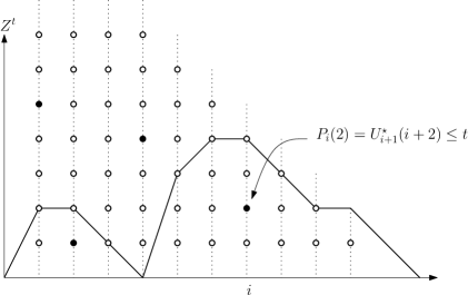
Figure 3: $Z^{t}$ and the field $(P^{n}_{i}(j))$ is represented by the bullets; the black ones are the ones whose value is at most $t$. So here, the graph represented has two connected components, each having one extra edge.

References

- Addario-Berry et al. [2012] L. Addario-Berry, N. Broutin, and C. Goldschmidt. The continuum limit of critical random graphs. Probability Theory and Related Fields, 152:367–406, 2012.
- Aldous [1991] D. Aldous. The continuum random tree. I. The Annals of Probability, 19:1–28, 1991.
- Aldous [1997a] D. Aldous. Brownian excursions, critical random graphs and the multiplicative coalescent. The Annals of Probability, 25(2):812–854, 1997a.
- Aldous and Pitman [1998] D. Aldous and J. Pitman. The standard additive coalescent. The Annals of Probability, 26:1703–1726, 1998.
- Aldous [1997b] D. J. Aldous. Deterministic and stochastic models for coalescence (aggregation, coagulation): a review of the mean-field theory for probabilists. Bernoulli, 5:3–48, 1997b.
- Armendariz [2001] I. Armendariz. Brownian excursions and coalescing particle systems. Phd thesis, New York University, 2001.
- Bertoin [2000] J. Bertoin. A fragmentation process connected to brownian motion. Probability Theory and Related Fields, 117(2):289–301, 2000.
- Bertoin [2006] J. Bertoin. Random fragmentation and coagulation processes. Cambridge University Press, Cambridge, 2006.
- Bhamidi et al. [2013a] S. Bhamidi, A. Budhiraja, and X. Wang. Aggregation models with limited choice and the multiplicative coalescent. Random Structures and Algorithms, 2013a. to appear.
- Bhamidi et al. [2013b] S. Bhamidi, A. Budhiraja, and X. Wang. The augmented multiplicative coaslescent, bounded size rules and critical dynamics of random graphs. Probability Theory and Related Fields, 2013b. To appear.
- Bollobás [2001] B. Bollobás. Random Graphs. Cambridge Studies in Advanced Mathematics. Cambridge University Press, second edition, 2001.
- Chandler et al. [1982] R. Chandler, K. Lerman, J. Koplik, and J.F. Willemsen. Capillary displacement and percolation in porous media. Journal of Fluid Mechanics, 119:249–267, 1982.
- Chassaing and Louchard [2002] P. Chassaing and G. Louchard. Phase transition for parking blocks, brownian excursion and coalescence. Random Struct. Algorithms, 21(1):76–119, 2002.
- Donsker [1952] M.D. Donsker. Justification and extension of Doob’s heuristic approach to the Kolmogorov-Smirnov theorems. The Annals of Mathematical Statistics, 23:277–281, 1952.
- Evans and Pitman [1998] S.N. Evans and J. Pitman. Construction of Markovian coalescents. Annales de l’Institut Henri Poincaré: Probabilités et Statistiques, 34:339–383, 1998.
- Fournier and Laurençot [2006] N. Fournier and P. Laurençot. Well-posedness of Smoluchowski’s coagulation equation for a class of homogeneous kernels. Journal of Functional Analysis, 233(2):351 – 379, 2006.
- Fournier and Löcherbach [2009] N. Fournier and E. Löcherbach. Stochastic coalescence with homogeneous-like interaction rates. Stochastic Processes and their Applications, 119(1):45–73, 2009.
- Janson et al. [2000] S. Janson, T. Łuczak, and A. Ruciński. Random Graphs. Wiley, New York, 2000.
- Jarník [1930] V. Jarník. O jistém problému minimálním. Práce Mor. Přírodověd. Spol. v Brně (Acta Societ. Scient. Natur. Moravicae), 6:57–63, 1930.
- Kaigh [1976] W.D. Kaigh. An invariance principle for random walk conditioned by late return to zero. The Annals of Probability, 4:115–121, 1976.
- Kallenberg [2002] O. Kallenberg. Foundations of modern probability. Probability and its applications. Springer, New York, 2002.
- Le Gall [2005] J.-F. Le Gall. Random trees and applications. Probability Surveys, 2:245–311, 2005.
- Lenormand and Bories [1980] R. Lenormand and S. Bories. Description d’un mécanisme de connexion de liaision destiné a l’étude du drainage avec piégeage en milieu poreux. C.R. Acad. Sci. Paris, 291:279–282, 1980.
- Lushnikov [1978] A.A. Lushnikov. Some new aspects of coagulation theory. Izv. Atmos. Ocean Phys., 14:738–743, 1978.
- Marckert [2008] J.-F. Marckert. One more approach to the convergence of the empirical process to the Brownian bridge. Electronic Journal of Statistics, 2:118–126, 2008.
- Marcus [1968] A.H. Marcus. Stochastic coalescence. Technometrics, 10(1):133–143, 1968.
- Pitman [1999] J. Pitman. Coalescent random forests. Journal of Combinatorial Theory, Series A, 85:165–193, 1999.
- Pitman [2006] J. Pitman. Combinatorial stochastic processes, volume 1875 of Lecture Notes in Mathematics. Springer, Berlin, 2006.
- Prim [1957] R. C. Prim. Shortest connection networks and some generalizations. Bell Syst. Tech. J., 36:1389–1401, 1957.
- Smoluchowski [1916] M.V. Smoluchowski. Drei Vortrage uber Diffusion, Brownsche Bewegung und Koagulation von Kolloidteilchen. Physik. Zeit., 17:557–585, 1916.