Confined flow of suspensions modeled by a frictional rheology

Abstract

We investigate in detail the problem of confined pressure-driven laminar flow of neutrally buoyant non-Brownian suspensions using a frictional rheology based on the recent proposal of Boyer et al. (2011a). The friction coefficient (shear stress over particle normal stress) and solid volume fraction are taken as functions of the dimensionless viscous number $I$ defined as the ratio between the fluid shear stress and the particle normal stress. We clarify the contributions of the contact and hydrodynamic interactions on the evolution of the friction coefficient between the dilute and dense regimes reducing the phenomenological constitutive description to three physical parameters. We also propose an extension of this constitutive framework from the flowing regime (bounded by the maximum flowing solid volume fraction) to the fully jammed state (the random close packing limit).

We obtain an analytical solution of the fully-developed flow in channel and pipe for the frictional suspension rheology. The result can be transposed to dry granular flow upon appropriate redefinition of the dimensionless number $I$. The predictions are in excellent agreement with available experimental results for neutrally buoyant suspensions, when using the values of the constitutive parameters obtained independently from stress-controlled rheological measurements. In particular, the frictional rheology correctly predicts the transition from Poiseuille to plug flow and the associated particles migration with the increase of the entrance solid volume fraction.

We also numerically solve for the axial development of the flow from the inlet of the channel/pipe toward the fully-developed state. The available experimental data are in good agreement with our numerical predictions, when using an accepted phenomenological description of the relative phase slip obtained independently from batch-settlement experiments. The solution of the axial development of the flow notably provides a quantitative estimation of the entrance length effect in pipe for suspensions when the continuum assumption is valid. Practically, the latter requires that the predicted width of the central (jammed) plug is wider than one particle diameter. A simple analytical expression for development length, inversely proportional to the gap-averaged diffusivity of a frictional suspension, is shown to encapsulate the numerical solution in the entire range of flow conditions from dilute to dense.

Keywords

Granular media, suspensions, porous media, particle/fluid flow

1 Introduction

Phenomenology of non-Brownian suspension flow distinguishes between several regimes based on the value of the solid volume fraction $\phi$: dilute, concentrated, and dense as the “flowing” limit $\phi\rightarrow\phi_{m}$ is approached (e.g. Stickel and Powell, 2005). In the dilute regime $(\phi\lesssim 0.2)$, the mixture behaves as a Newtonian fluid whose apparent viscosity is a slowly increasing function of the solid volume fraction (Einstein, 1906; Batchelor and Green, 1972), and the normal stress components acting on the solid phase, hereafter referred to as the particle or effective normal stresses, are negligible (e.g. Stickel and Powell, 2005). The upper bound of the dilute regime appears to be related to the percolation threshold for a transient cluster (De Gennes, 1979). Above this threshold, i.e. in the concentrated regime, suspension develops distinct compressive particle normal stress (Deboeuf et al., 2009; Dbouk et al., 2013b), and the apparent viscosity of the mixture increases significantly with the solid volume fraction (Krieger and Dougherty, 1959). No relative slip between the fluid and solid phases for low Reynolds number flows has been measured in this regime to the accuracy of the experimental methods (Lyon and Leal, 1998a; Isa et al., 2010). For yet larger solid volume fraction, approaching the jamming/flowing transition $\phi\rightarrow\phi_{m}$, the apparent viscosity diverges, and a finite frictional yield stress is approached in this limit even when the base fluid is strictly Newtonian. The reported values for the flowing limit of mono-disperse suspensions, $\phi_{m}\approx 0.585$ in the effective stress controlled experiments of Boyer et al. (2011a) and $\phi_{m}\approx 0.605$ from the local MRI measurements of Ovarlez et al. (2006), are distinctly lower than the random close packing value $\phi_{\mathrm{rcp}}\approx 0.63-0.64$. Above the flowing limit ($\phi>\phi_{m}$), the macroscopic solid velocity is zero and the medium behaves as a porous granular solid, through which the base fluid phase can percolate. In that limit, the relative phase slip governs pore fluid pressure diffusion “a la Darcy” (Bear, 1972).

Recently, dense suspension rheology has been investigated experimentally by (Boyer et al., 2011a) under conditions of a simple shear flow at a fixed applied particle normal stress $-\sigma_{n}^{\prime}$ (with the convention of positive stress in tension). Their results indicate that the suspension exhibits an apparent shear-thinning behaviour under constant particle normal stress conditions (i.e. the apparent viscosity decreases with the shear-rate). This behaviour is to be contrasted with an apparent Newtonian behaviour when the solid volume fraction is imposed and the particle normal stress is allowed to vary (increase) with the shear-rate. Boyer et al. (2011a) further show that suspensions, akin to dry granular media, can be phenomenologically described by a viscoplastic frictional rheology, fully characterized by the dependence of the friction coefficient $\mu=\tau/(-\sigma_{n}^{\prime})$ and the volume fraction $\phi$ on a dimensionless viscous number (Cassar et al., 2005)

$$I=\frac{\eta_{f}\dot{\gamma}}{-\sigma_{n}^{\prime}}$$

which contrasts the relative magnitudes of the viscous shear stress $\eta_{f}\dot{\gamma}$ ($\eta_{f}$ is the viscosity of the base fluid and $\dot{\gamma}$ is the macroscopic shear rate) and the particle normal stress $-\sigma_{n}^{\prime}$, respectively. The friction coefficient $\mu(I)$ evolves from a static value $\mu_{1}$ in the jamming limit $I=0$ of a dense suspension to a diverging value $\sim I+\frac{5}{2}\phi_{m}I^{1/2}$ for large $I$ in a dilute flow. This evolution spans the range of behaviors from the pressure-dependent frictional granular solid in the dense limit, $\tau=-\mu_{1}\sigma_{n}^{\prime}$, to the Newtonian fluid in the dilute limit, $\tau=\eta_{f}\dot{\gamma}$.

In this work, we review the frictional suspension rheology and consider an extension from the flowing regime to the jammed, non-flowing state. We point out that such an extension is necessary to model pressure-driven suspension flows, which are characterized by the existence of a jammed central “plug”, and to our knowledge has not been explicitly recognized in previous modeling attempts. We propose that non-flowing material compacts with the decreasing stress ratio, from the maximum flowing solid volume fraction $\phi_{m}$ at the flow threshold $\mu=\mu_{1}$ to the random close packing value $\phi_{rcp}$ at $\mu\sim 0$. The compaction of the non-flowing pack is formally similar to the dilatant/compactive behavior of the flowing material. However, the driving mechanisms behind the flowing and non-flowing compaction have to be distinct. In the former, the macroscopic shear flow enables changes of the particle pack, while in the latter, non-flowing packs, we hypothesize that microscopic, “in-cage” particle rearrangements are enabled by the velocity/pressure fluctuations in the surrounding flowing material. Notwithstanding the origin of the fluctuations, the latter mechanism appears to be similar to the compaction of a static granular pack in tapping and cyclic shear experiments (e.g. Knight et al., 1995; Pouliquen et al., 2003).

We use the extended frictional rheology to obtain solution for pressure-driven flow in a channel and a pipe of a non-Brownian, neutrally buoyant suspension of hard mono-dispersed spheres in a Newtonian liquid under the condition of negligible inertia. Such type of flows has been extensively investigated both experimentally (Karnis et al., 1966; Leighton and Acrivos, 1987; Sinton and Chow, 1991; Lyon and Leal, 1998a; Hampton et al., 1997) and theoretically with suspensions balance models (Nott and Brady, 1994; Mills and Snabre, 1995; Fang et al., 2002; Miller and Morris, 2006; Dbouk et al., 2013a; Ramachandran and Leighton, 2008; Ramachandran, 2013) among others. In such confined flow, the velocity profile transitions from a Poiseuille to plug-like shape when the entrance solid volume fraction increases. The frictional rheology has the advantage of combining the existence of a yield stress, which value depends on the magnitude of the particle normal stress, and the evolution of the shear and normal viscosities with solid volume fraction, similar to suspension balance models. It is therefore of interest to test its prediction on pressure-driven flow for which experimental results for velocity and solid volume fraction profiles across the gap are available in the literature. We develop an analytic solution for the fully-developed flow, and then study numerically how the flow evolves with distance from the inlet of the channel or pipe towards the fully-developed state. The predictions based on these solutions compare very well to the published experimental results. Importantly, these comparisons are drawn for the solutions which are devoid of any matching parameters, i.e. the constitutive parameters of the frictional rheology are identified independently from rheological experiments of Boyer et al. (2011a) and a phenomenological description of the intrinsic solid-pack permeability function (or, alternatively, sedimentation hindrance function) is based on existing extensive compilations of fluidization and batch settlement experiments (Garside and Al-Dibouni, 1977; Davis and Acrivos, 1985).

To aid with navigating this paper’s notation, we acknowledge that starting with Section 4 (formulation for flow in a channel) and onwards, we make use of the normalized field variables, using scales defined by (19)-(21). A recourse back to the dimensional form of these variables, where not obvious, is explicitly acknowledged.

2 Continuum model for dense suspension/ wet granular media

2.1 Conservation laws

As already defined, $\phi$ is the solid volume fraction, $\boldsymbol{v}^{f}$ and $\boldsymbol{v}^{s}$ are the local average fluid and solid Eulerian velocities, respectively, and $\boldsymbol{u}=\phi\boldsymbol{v}^{s}+(1-\phi)\boldsymbol{v}^{f}$ is the mixture velocity. We assume that both fluid and solid constituents are incompressible (taken separately). The continuity equations for the solid phase and the mixture are then, respectively,

$$\frac{\partial\phi}{\partial t}+\nabla\cdot(\phi\boldsymbol{v}^{s}) = 0$$ (1)

$$\nabla\cdot\boldsymbol{u}=\nabla\cdot(\boldsymbol{q}+\boldsymbol{v}^{s}) = 0$$ (2)

where a relative phase slip velocity (with respect to the solid velocity) was introduced (Bear, 1972)

$$\boldsymbol{q}=(1-\phi)\left(\boldsymbol{v}^{f}-\boldsymbol{v}^{s}\right)=\boldsymbol{u}-\boldsymbol{v}^{s}$$

It will be convenient to also use an alternative form of the solid phase continuity, which is referred to as the consolidation equation in the porous media literature (e.g., Bear, 1972),

$$\frac{1}{\phi}\frac{d^{s}\phi}{dt}=\nabla\cdot\boldsymbol{q}$$ (3)

where $d^{s}\phi/dt=\partial\phi/\partial t+\boldsymbol{v}^{s}\cdot\nabla\phi$ is the solid material time derivative.

2.1.1 Balance of momentum, drag force

Neglecting inertial terms, the balance of the mixture momentum, in the absence of body forces, reduces to:

$$\nabla\cdot\boldsymbol{\sigma}=\boldsymbol{0}$$ (4)

where the total stress tensor $\boldsymbol{\sigma}=\boldsymbol{\sigma}^{f}+\boldsymbol{\sigma}^{\prime}$ is the sum of the fluid $\boldsymbol{\sigma}^{f}$ and particle (effective) $\boldsymbol{\sigma}^{\prime}$ stress tensors (von Terzaghi, 1940). In the remainder of this paper, we will make use of the fluid ($p^{f}$), particle ($p^{\prime}$), and mixture ($p=p^{f}+p^{\prime}$) pressure, defined as the respective mean stress value taken positive in compression, and of the mixture stress-deviator tensor $\boldsymbol{\tau}=\boldsymbol{\sigma}+p\boldsymbol{I}$.

In addition to (4), the balance of momentum of either the fluid or solid phases is needed to describe the two-phase continuum. For the fluid phase (see (Jackson, 2000) for more details),

$$(1-\phi)\nabla\cdot\boldsymbol{\sigma}^{f}-\boldsymbol{F}=\boldsymbol{0}$$

where the force $\boldsymbol{F}$ is the total interaction force between the solid and fluid phases, besides the buoyancy $\phi\nabla\cdot\boldsymbol{\sigma}^{f}$. For negligible Reynolds number, the latter is limited to drag force, which is proportional to the phase slip velocity (Bear, 1972)

$$\boldsymbol{F}=(1-\phi)\frac{\eta_{f}}{k(\phi)}\boldsymbol{q}\quad\text{with}\quad k(\phi)=a^{2}\kappa(\phi),$$ (5)

where $k$ is the intrinsic permeability of the solid particles assembly, $\kappa$ its normalized form, $a$ the particle size (radius), and $\eta^{f}$ the fluid viscosity. The combination of the fluid phase balance of momentum and the expression for the drag force gives:

$$\boldsymbol{q}=\frac{a^{2}\kappa(\phi)}{\eta_{f}}\nabla\cdot\boldsymbol{\sigma}^{f}$$ (6)

which is further reduced to Darcy’s law under the assumption of negligible fluid shear stress ($\boldsymbol{\sigma}^{f}\approx-p^{f}\boldsymbol{I}$). For granular porous media, a classic choice for the permeability dependence on the solid volume fraction is given by the Kozeny-Carman law $\kappa(\phi)=(1-\phi)^{3}/45\phi^{2}$ (Kozeny, 1927; Carman, 1937).

In the suspension rheology literature, the balance of momentum for the solid phase is used instead to derive an expression for the particle slip velocity with respect to the bulk, $\boldsymbol{v}^{s}-\boldsymbol{u}=-\boldsymbol{q}$, (e.g., Jackson, 2000), which in the absence of body forces has the form:

$$-\boldsymbol{q}=\frac{2a^{2}}{9\eta_{f}}\frac{f(\phi)}{\phi}\nabla\cdot\boldsymbol{\sigma}^{\prime}$$ (7)

where $f(\phi)$ is the sedimentation hindrance function, evaluated in batch sedimentation ($\boldsymbol{\sigma}^{\prime}=\boldsymbol{u}=0$) as the ratio of the particle settling velocity in the suspension to the terminal settling velocity of a single particle in clear fluid.

The two formalisms (equations (6) and (7)) are equivalent in view of (4) when the scaled permeability $\kappa(\phi)$ is uniquely related to the hindrance function $f(\phi)$,

$$\kappa(\phi)=\frac{2}{9}\frac{f(\phi)}{\phi}$$ (8)

A particularly simple empirical form of the hindrance function, $f(\phi)=\left(1-\phi\right)^{\alpha}$ with $\alpha=4.65$, was proposed by Richardson and Zaki (1954) based on a number of fluidization experiments at low Reynolds numbers. The value of the exponent was later slightly revised to $\alpha=5.1$ by Garside and Al-Dibouni (1977) (see also Davis and Acrivos (1985)) based on the extensive study of fluidization and batch settlement experimental data available at the time. Figure 1 exemplifies how remarkably well the Richardson-Zaki phenomenology with $\alpha=5.1$ reproduces the experimental results of Bacri et al. (1986), obtained using very accurate acoustic measurements of sedimentation fronts, and the results of the direct numerical calculations of transport properties from dispersion of hard spheres (Ladd, 1990). The expressions of Kozeny-Carman and Mills and Snabre (1994), respectively, as well as the Richardson-Zaki relations with $\alpha=2$ and $\alpha=4$, are also shown in figure 1 for comparison purposes.

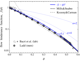
Figure 1: Different phenomenological expressions for the hindrance function $f(\phi)$ in log-linear scale (with the corresponding normalized permeability function given by $\kappa(\phi)=2f(\phi)/9\phi$) are contrasted to the data from batch sedimentation experiments (Bacri et al., 1986), and from the numerical simulations of the dispersion of hard spheres (Ladd, 1990). The Richardson and Zaki (1954) empirical form, $f=(1-\phi)^{\alpha}$ with $\alpha=5.1$ (Garside and Al-Dibouni, 1977; Davis and Acrivos, 1985), and Mills and Snabre (1994) theoretical expression, $f=(1-\phi)/(1+4.6\phi/(1-\phi)^{3})$, are in excellent agreement with both the experimental and numerical data over the entire (flowing) range of the solid volume fraction. Kozeny-Carman’s expression, $f=(1-\phi)^{3}/10\phi$, provides an adequate approximation of the sedimentation data for all but dilute ($\phi\lesssim 0.1$) suspensions.

2.2 Frictional rheology

In the rheology of suspension, constitutive relations for the evolution of the shear $\eta_{s}$ and normal $\eta_{n}$ viscosities of the mixture as function of the solid volume fraction $\phi$ are often used in so called suspension balance models (Morris and Boulay, 1999; Zarraga et al., 2000; Miller and Morris, 2006). Here, we use the frictional rheology proposed by Boyer et al. (2011a) to describe the constitutive behavior of dense suspension. Such a constitutive model is akin to a frictional viscoplastic law. A similar frictional framework has been successfully proposed for dry granular flow in the liquid regime (MiDi, 2004; Forterre and Pouliquen, 2008; Jop et al., 2006, and references therein).

For such a complex two-phase fluid, the effective stress, shear stress, shear rate, and solid volume fraction are intrinsically related, and only two of these four field variables can be prescribed independently. For a simple shear flow, Boyer et al. (2011a) write a frictional relation for the mixture shear stress and the effective (particle) confining stress and an evolution of the solid volume fraction as

$$\tau=\mu(I)\,(-\sigma_{n}^{\prime})\qquad\phi=\phi(I)$$ (9)

where macroscopic friction coefficient $\mu$ and the solid volume faction $\phi$ are functions of the viscous number $I$, defined as a ratio of the viscous shear stress in the fluid to the particle confining stress,

$$I=\frac{\eta_{f}\dot{\gamma}}{-\sigma^{\prime}_{n}}$$ (10)

This number was originally proposed by Cassar et al. (2005) based on a micro-mechanical consideration of timescales controlling the solid particles motion in a suspension. For large values of this dimensionless number, the stress transmitted through short-range particle interactions (contacts, lubrication), which, we further refer to as “contacts” for brevity, is negligible compared to the fluid viscous stress: hydrodynamics interactions dominate the behavior of the suspension. This limit corresponds to the dilute regime. On the contrary, for small $I$, short-range particle interactions dominate the suspension behavior and the macroscopic friction coefficient tends to a constant thus defining an effective pressure-dependent yield stress. Based on rheological experiments performed under effective normal stress control on two different suspensions of mono-disperse spheres in Newtonian fluid, Boyer et al. (2011a) propose the following phenomenological relation for the friction coefficient as a function of the viscous number:

$$\mu(I)=\underbrace{\mu_{1}+\frac{\mu_{2}-\mu_{1}}{1+I_{0}/I}}_{\mu^{cont}}+\underbrace{I+\frac{5}{2}\phi_{m}I^{1/2}}_{\mu^{hydro}}$$ (11)

This law combines a contribution from particle contacts $\mu^{cont}(I)$ similar to the one reported for dry granular media and a hydrodynamic contribution $\mu^{hydro}(I)$ designed to recover the behavior of the dilute regime. The second constitutive equation relates the solid volume fraction law to the viscous number $I$, and chosen by Boyer et al. (2011a) in the following form

$$\phi(I)=\frac{\phi_{m}}{1+I^{1/2}}$$ (12)

As can be seen from figure 2, relations (11)-(12) with $\mu_{1}=0.32$, $\mu_{2}=0.7$, $\phi_{m}=0.585$, and $I_{0}=0.005$ reproduce very well experimental results of Boyer et al. (2011a) and Dbouk et al. (2013b).

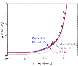
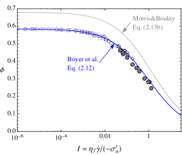
Figure 2: Selected frictional rheologies of a flowing suspension, which relate the stress ratio / friction coefficient $\mu$, solid volume fraction $\phi$, and the viscous number $I$, contrasted to experimental data of Boyer et al. (2011a), obtained for nearly mono-dispersed suspensions in annular shear cell under effective stress control ($\circ$, $\square$, $\diamond$), and Dbouk et al. (2013b), obtained in a parallel plate rheometer with local pressure measurements ($\bullet$).

As shown by Boyer et al. (2011a), a frictional rheology (9) with (10) is formally equivalent to suspension balance rheology (e.g., Morris and Boulay, 1999; Stickel and Powell, 2005)

$$\tau=\eta_{f}\eta_{s}(\phi)\dot{\gamma}\qquad{{\sigma^{\prime}_{n}=-\eta_{f}\eta_{n}(\phi)\dot{\gamma}}}$$

when the relative shear and normal viscosities are expressed as $\eta_{s}=\mu(I)/I$ and $\eta_{n}=1/I$, respectively, and $I=I(\phi)$, (9). The shear and normal viscosity functions of the solid volume fraction proposed in the literature (e.g. Krieger and Dougherty, 1959; Morris and Boulay, 1999; Boyer et al., 2011a) diverge when $\phi$ tends toward $\phi_{m}$ (i.e. when the shear rate tends to zero), highlighting the presence of a frictional yield stress, as intrinsically present in the frictional rheology. The ratio of the two suspension viscosities defines the friction coefficient, i.e. $\mu=\eta_{s}/\eta_{n}$. A frictional yield stress will thus be present only if $\lim_{\phi\rightarrow\phi_{m}}\eta_{s}(\phi)/\eta_{n}(\phi)$ tends to a finite constant, i.e. if the two viscosities diverge at the same rate $\sim 1/I(\phi)$,e.g. $\sim(\phi_{m}-\phi)^{-2}$ per (12).

Along the above lines, the rheology of Morris and Boulay (1999) (see also Fang et al., 2002; Miller and Morris, 2006) provide an example of suspension-balance rheology characterized by a finite frictional yield stress. Indeed, their rheology can be shown to be equivalent to

$$\mu(I)=\underbrace{\mu_{1}}_{\mu^{cont}}+\underbrace{I+\frac{5}{2}\phi_{m}\frac{I^{1/2}}{K_{n}^{1/2}}}_{\mu^{hydro}}\qquad\phi(I)=\frac{\phi_{m}}{1+K_{n}^{1/2}I^{1/2}}$$ (13)

where $\mu_{1}=0.133$, $K_{n}=0.75$, and $\phi_{m}=0.68$ are used by these authors to fit their model predictions to wide-gap Couette flow data of Phillips et al. (1992). (Note that the authors make use of the parameter $K_{s}=\mu_{1}K_{n}$ instead of $\mu_{1}$). The rheology (13) is qualitatively similar to that of Boyer et al. (2011a) (equations (11)-(12)) with one significant distinction being in the contribution of particle contacts to friction ($\mu^{cont}$). For the rheology of Morris and Boulay (1999), $\mu^{cont}$ is a constant given by the jamming value $\mu_{1}$, while for the experimentally-derived rheology of Boyer et al. (2011a), $\mu^{cont}$ is increasing with $I$ from the minimum value $\mu_{1}$ at $I=0$. Figure 2 shows that, although the two rheologies are qualitatively similar, the rheology of Morris and Boulay (1999) does not represent the experimental data very well quantitatively, which can be tracked to their choice of the jamming values of the solid volume fraction (overestimated $\phi_{m}$) and the friction coefficient (underestimated $\mu_{1}$), as well as the lack of dependence of their contact contribution $\mu^{cont}$ on the viscous number.

2.2.1 Alternative form of the friction expression

Although the functional form (11) of the friction law $\mu(I)$ proposed by Boyer et al. (2011a) provides a very good match to the experimental data, we do observe a slight inconsistency between their functional form and the interpretation of $\mu^{cont}$ and $\mu^{hydro}$ as the terms contributing to the total friction coefficient $\mu=\mu^{cont}+\mu^{hydro}$ from physically distinct “contact” and “hydrodynamic” interactions between the particles in a suspension, respectively. (This distinction may be blurred in the intermediate flowing regime, but is apparent in the two end member regimes corresponding to $\phi\rightarrow\phi_{m}$ and $\phi\rightarrow 0$, respectively). Specifically, the departure of the friction coefficient from the jamming limit ($\mu=\mu_{1}$ at $I=0$) with increasing shear rate in Boyer et al. framework, $\mu-\mu_{1}=\frac{5}{2}\phi_{m}I^{1/2}+O(I)$, is given by the Einstein’s term. This appears to be at odds with the physical origin of the Einstein’s term which lies in the suspension’s dilute limit.

We suggest to model the contact dominated response of a dense suspension, $\mu^{cont}$, by a simple linear dependence on the solid volume fraction

$$\mu^{cont}=\mu_{1}+\frac{\phi_{m}-\phi}{\beta}$$ (14)

where $\beta=-(d\phi/d\mu)^{cont}$ is a “compressibility” coefficient. This linear relation with

$$\phi_{m}=0.585\qquad\mu_{1}=0.3\qquad\beta=0.158$$

provides an excellent approximation to the available data when recasted onto the ($\phi,\mu$) plane on figure 3. Importantly, a linear relation between $\mu$ and $\phi$ in the dense regime has also been corroborated for dense dry granular media in numerical 2D simple shear experiments (da Cruz et al., 2005; Rognon et al., 2008) and in the laboratory (Craig et al., 1986). A friction law, which is not limited to the dense regime, is then put together similarly to Boyer et al. (2011a) by adding a “hydrodynamic” interactions term to the “contact” ones,

$$\mu(\phi)=\underbrace{\mu_{1}+\frac{\phi_{m}}{\beta}\left(1-\frac{\phi}{\phi_{m}}\right)}_{\mu^{cont}}+\underbrace{\left(I(\phi)+\left(\frac{5}{2}\phi_{m}+2\right)I(\phi)^{1/2}\right)\left(1-\frac{\phi}{\phi_{m}}\right)^{2}}_{\mu^{hydro}}$$ (15)

and adopting Boyer et al.’s relation (12) between the viscous number and the solid volume fraction,

$$I(\phi<\phi_{m})=(\phi_{m}/\phi-1)^{2}\quad\text{and}\quad I(\phi\geq\phi_{m})=0.$$ (16)

We comment on the form of $\mu^{hydro}$ in (15) which is similar to the Boyer’s $\mu^{hydro}$ in the dilute limit ($\phi\rightarrow 0$ or $I\rightarrow\infty$), which in itself is equivalent to the Einstein’s correction. This dilute limit is weighted by a quadratic prefactor $\sim(\phi_{m}-\phi)^{2}$ in (15) in order to enforce the dominance of the “contacts” interactions (14) in the dense regime, i.e. $\mu=\mu^{cont}(\phi)+O(\phi_{m}-\phi)^{3}$.

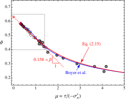
(a)(b)

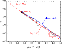
Figure 3: Solid volume fraction $\phi$ vs. stress ratio $\mu=\tau/{(-\sigma_{n}^{\prime})}$, (a), for the selected frictional rheologies contrasted to the experimental data of Boyer et al. (2011a) and Dbouk et al. (2013b). Dotted line shows a linear fit with the slope of $\beta\approx 0.158$ to the experimental data in the dense regime (see also the close-up of this regime shown in (b)), which is identified with the contribution of particle contacts to friction, $\mu^{cont}(\phi)$, in rheology Eq. (15), shown by solid red line. The latter rheology allows simple (linear) continuation into the jammed regime ($\phi_{m}<\phi<\phi_{rcp}$), where solid fraction relaxes to the maximum value $\phi_{rcp}\approx 0.632$ with either decreasing shear stress or increasing effective mean stress.

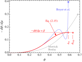
Figure 4: Inelastic “compressibility” parameter $(-d\phi/d\mu)$ as a function of a flowing solid volume fraction $\phi<\phi_{m}$ for three frictional rheologies, as in figure 2. Corresponding jamming points are shown by a cross. The modification of the Boyer et al.’s rheology (Eq. (15), red line) regularizes the latter in the dense flowing regime, and allows simple continuation into the jammed regime ($\phi_{m}<\phi<\phi_{rcp}$) using the asymptotic compressibility $\beta=0.158$ (dotted line).

Similarly to the original Boyer’s rheological expression (11), the framework (15) provides a very good match to the experimental data (figures 2 and 3), and, as to be seen in Section 4, the two constitutive frameworks yield close quantitative predictions for the fully-developed suspension flow in a channel or a pipe for all but very dense flows (with average $\phi\gtrsim 0.5$). One can thus legitimately wonder whether this “fine-tuning” of the frictional rheology is at all necessary. In fact, the advantage of the alternative frictional description becomes fully apparent when considering the axial flow development. It is to be shown in section 5 that, similarly to previous studies using suspension balance models, the flow development is driven by the cross diffusion of the particle normal stress. This stress diffusion is governed by the “hydraulic conductivity” $k(\phi)/\eta_{f}$ and the “compressibility” parameter of the suspension $(-d\phi/d\mu)$. The latter is shown on figure 4 for the original Boyer et al. (2011a) and the modified frictional models. Clearly, the expression (13) proposed by Boyer et al. (2011a) results in a seemingly degenerate behavior of the compressibility parameter in the dense regime, which impacts the flow axial development prediction and hinder the numerical treatment of the problem.

2.2.2 Extension to non-flowing state

In writing constitutive equations in the form (15-16), we effectively extended the linear relation between the solid volume fraction and the stress ratio $\mu$, found experimentally in the dense flowing regime, to the jammed state ($\phi>\phi_{m}$). We can find the corresponding maximum value of the solid fraction that can be achieved if the stress ratio is allowed to vanish in this constitutive description, $\phi\rightarrow\phi_{m}+\beta\mu_{1}\approx 0.632\approx\phi_{rcp}$ as $\mu=-\tau/\sigma^{\prime}_{n}\rightarrow 0$ (where we have used $\phi_{m}=0.585$, $\beta=0.158$, and $\mu_{1}=0.3$ as corroborated before). This value is conspicuously similar to the random-close-packing value $\phi_{rcp}$ for mono-dispersed spheres, estimated in the range between 0.63 and 0.64 (e.g., Scott and Kilgour, 1969; Berryman, 1983). We therefore hypothesize that the random close packing in the jammed part of otherwise flowing granular system can be achieved by either increasing particle normal stress(to infinity) while maintaining fixed, non-zero value of the shear stress, or by decreasing the shear stress to zero while maintaining a non-zero value of the particle normal stress. This response of the model is not inconsistent with what we usually think of the relaxation of the jammed solid fraction from an initially flowing state. In foreseen applications of suspension flow in various geometries, the jammed region of the flow is constantly excited by perturbations from the nearby flowing region, similar to tapping, vibrations or particle pressure / velocity fluctuations that are usually used to achieve closed packing from an initially loose jammed state in experiments (e.g. Knight et al., 1995; Pouliquen et al., 2003). Thus, we can infer with this model that the jammed state subjected to particle pressure fluctuations will evolve to the solid volume fraction value defined by the imposed macroscopic stress ratio, $\phi=\phi(\mu)$. We are not aware of any laboratory or numerical experiments that would try to quantify the dependence of the solid fraction in a jammed system of rigid particles on the imposed macroscopic $\mu$ (that would prove or disprove our proposal), but this issue can be probed by looking at solid fraction variation within a plug of otherwise flowing systems (such as pressure or gravity driven flow in a channel or pipe). As we will show in Section 4.5, when the resolution of experimental methods allow (Hampton et al., 1997), one can observe a solid fraction gradient in the plug region of a pressure-driven flow consistent with our jammed rheology and inferred values of the stress ratio gradient across the plug.

We also note that the random close packing has been approached in the limit of non-zero stress ratio $\mu(\phi_{\mathrm{rcp}})\sim 0.1$ in the numerical simulation of flowing (simple shear) dry granular system of frictionless particles (Peyneau and Roux, 2008). This may indicate that our assumption of vanishing $\mu(\phi_{\mathrm{rcp}})$ may not be fully accurate. Accepting for a moment that $\mu(\phi_{\mathrm{rcp}})>0$, would result in a finite region at the random close packing (where the stress ration is $0\leq\mu\leq\mu(\phi_{\mathrm{rcp}})$) within the broader jammed plug ($0\leq\mu\leq\mu(\phi_{\mathrm{m}})$) in a pressure-driven flow in a confined geometry. This is to be compared to a single point where the random close packing is reached within the plug when $\mu(\phi_{\mathrm{rcp}})=0$ is assumed. Resolution of the solid volume fraction measurements within a plug in the existing pressure-driven flow experiments is insufficient to eliminate either possibility, and, thus, we settle for $\mu(\phi_{\mathrm{rcp}})=0$ in this work.

Accounting for the inelastic compaction beyond the flowing regime, suggests that formulation of the frictional rheology using the solid volume fraction $\phi$, as the main state variable, i.e. $\mu=\mu(\phi)$ and $I=I(\phi)$, where $\phi$ spans both flowing ($I>0,\,\phi<\phi_{m}$) and non-flowing ($I=0,\,\phi_{m}<\phi<\phi_{rcp}$) regimes, may be a preferred form over the one using $I$ as the main state variable. Equations (15-16), which provide a particular form of this rheology, contain only three independent parameters, namely, values of the solid fraction, stress ratio, and compressibility $(-d\phi/d\mu)$ at the jamming transition, $\phi_{m}$, $\mu_{1}$, and $\beta$, respectively. Furthermore, in view of the proposed relation between these parameters and the random-close-packing limit, the system can be alternatively parametrized by values of the solid volume fraction and compressibility at random-close-packing, $\phi_{rcp}$ and $\beta$, respectively, and by $\phi_{m}$ (or $\mu_{1}=(\phi_{rcp}-\phi_{m})/\beta$) at the jamming transition.

2.2.3 Transient Effects

The constitutive framework discussed so far pertains to a “steady-state” flow, which assumes that the internal relaxation time of the system in response, for example, to a change of the macroscopic shear rate is small compared to the timescale of this change. One such relaxation process is transient inelastic dilatancy/contraction, as may occur, for example, in the beginning or cessation of the flow. As inspired by critical state soil mechanics Muir Wood (1990), the evolution of the system to a new steady-state can be described by an evolution law for the transient solid volume fraction development of the form (Pailha and Pouliquen, 2009)

$$\frac{1}{\phi}\frac{d^{s}\phi}{dt}\propto\dot{\gamma}\left[\phi_{cs}(I)-\phi\right]$$ (17)

where $\phi_{cs}(I)$ refers here to the “critical-state” solid volume fraction given by (12). For a pressure-driven flow in a channel or a pipe, the macroscopic timescale of axial flow development $t_{macro}\sim(L/H)/\dot{\gamma}$, where $H$ is the channel half-width (pipe radius) and $L\sim H^{3}/a^{2}\gg H$ is the axial development length (Nott and Brady, 1994). Consequently, the relaxation time $\sim 1/(\phi\dot{\gamma})$ associated with state evolution (17) is negligibly small compared to $t_{macro}$, pointing to the critical-state nature of this flow.

2.2.4 Normal Stress Differences

Neutrally buoyant non-Brownian suspensions are known to develop normal stress differences with increasing solid concentration (see, for example, Zarraga et al., 2000; Boyer et al., 2011b; Garland et al., 2013; Dbouk et al., 2013b). In the case of channel flow, normal stress differences do not impact the flow predictions when a frictional rheology linking the shear stress to the particle confining stress is assumed (see developments of Section 3). They may however play a role in pipe flow, especially at elevated bulk values of the solid volume fraction (see Miller and Morris (2006); Ramachandran (2013), and Appendix A). In our treatment of the pipe flow, to the first approximation, we neglect the effect of normal stress differences, while leaving more complete treatment of the problem to a future work.

2.2.5 Choice of kinematic variables

In the following, we will use the solid velocity $\boldsymbol{v}^{s}$ and the relative phase slip velocity $\boldsymbol{q}$ as the kinematic variables. Moreover, we express the frictional rheology as function of the solid shear rate. The choice of the solid shear rate to describe the kinematic of suspension deformation stems from the fact that in the dense regime, near jamming it is the only acceptable one in order to define a jammed state unambiguously while allowing the fluid to percolate through the jammed medium. Moreover, for dilute suspensions, the distinction between the fluid and solid shear rates is negligible for the case of non-inertial flow: i.e. phase slip is small in the dilute regime. We write thus the total stress in terms of the solid phase strain rate and write the law for the relative flux vector $\boldsymbol{q}$ neglecting the fluid shear stress compared to the “pore” fluid pressure $p^{f}$ (as it is typically done in porous media flow analysis). For the remainder of this paper, we thus drop the index “$s$” in the solid velocity and in the corresponding material time derivative for clarity and write: $\boldsymbol{v}^{s}=\boldsymbol{v}$ and $d^{s}/dt=d/dt$.

3 Formulation of channel flow

We now turn to the case of pressure-driven Stokesian flow of a suspension characterized by the previously described frictional rheology in a channel. Suspension flow in a circular pipe is amenable to a similar method of solution, which details are given in Appendix A.

3.1 Scaling

We denote as $U_{0}$ a characteristic axial velocity (set here to the entrance velocity value) of the flow in a channel with half-width $H$, a characteristic axial length $L$, and a characteristic aspect ratio of the channel (presumably small)

$$\delta=H/L$$ (18)

We assume plane flow such that the velocity is given $\boldsymbol{v}=v_{x}\boldsymbol{e_{x}}+v_{y}\boldsymbol{e_{y}}$, where the $y$ coordinate denotes the direction perpendicular to the channel axis. Since the constitutive laws for the suspension described previously are incrementally akin to a Newtonian fluid, we will use the classical Newtonian lubrication scaling (e.g., Frigaard and Ryan (2004)). We therefore introduce the following kinematic scales

$$t_{*}=\frac{L}{U_{o}}\qquad x_{*}=L\qquad y_{*}=H\qquad(v_{x})_{*}=U_{o}\qquad(v_{y})_{*}=\delta\,U_{o}\qquad\dot{\gamma}_{*}=\frac{U_{o}}{H}$$ (19)

shear/deviatoric stress ($\tau_{*}$), particle stress ($p_{*}^{\prime}$), total stress ($p_{*}$), and fluid pressure ($p_{*}^{f}$) scales

$$\tau_{*}=p_{*}^{\prime}=\frac{\eta_{f}U_{o}}{H}\qquad p_{*}=p_{*}^{f}=\frac{\tau_{*}}{\delta}$$ (20)

and relative phase velocity scale

$$q_{*}\equiv\frac{a^{2}}{\eta_{f}}\frac{p_{*}^{f}}{L}=\left(\frac{a}{H}\right)^{2}U_{o}$$ (21)

This scaling reflects the expectation that the velocity component across the channel, $v_{y}$, is much smaller (by $O(\delta)$) than the axial velocity, while the relative phase flux is more effective across the channel than along it. The stress scales suggest that the shear stress for pressure-driven flows is much smaller than the normal components of total stress and the pore pressure.

Finally, we choose the lengthscale $L$ to scale the axial flow development length, the entrance length of the flow over which the shear-driven particle migration across the channel leads to the fully-developed state. Significant particle migration across the channel during flow development requires that the relative phase cross-flux is comparable to the solid cross-flux, $q_{y}\sim v_{y}$, or, in view of their scales, (19) and (21), that aspect ratio $\delta=H/L$ is comparable to $(a/H)^{2}$. This is therefore equivalent to the Nott and Brady (1994) scaling argument prescribing the development lengthscale in the form

$$L=H^{3}/a^{2}$$ (22)

which is equivalent to setting $\delta=H/L=(a/H)^{2}$.

Hereafter, we will make use of the normalized field variables, using scales (19-21), while a recourse back to the dimensional form of these variables, where not obvious, will be explicitly acknowledged.

3.2 Normalized equations in scaling (19-21)

In the adopted scales, the normalized two component momentum balance for the mixture becomes

$$0 = \frac{\partial\tau_{xy}}{\partial y}-\frac{\partial p}{\partial x}+\delta\frac{\partial\tau_{xx}}{\partial x}$$ (23)

$$0 = -\frac{1}{\delta}\frac{\partial p}{\partial y}+\frac{\partial\tau_{yy}}{\partial y}+\delta\frac{\partial\tau_{xy}}{\partial x}$$ (24)

where both equations have been multiplied by $\delta$.

The expressions for the normalized components of the relative phase slip vector reduce to:

$$q_{x} = -\kappa(\phi)\frac{\partial p^{f}}{\partial x}=-\kappa(\phi)\left(\frac{\partial p}{\partial x}-\delta\frac{\partial p^{\prime}}{\partial x}\right)=-\kappa(\phi)\frac{\partial p}{\partial x}+O(\delta)$$ (25)

$$q_{y} = -\frac{\kappa(\phi)}{\delta}\frac{\partial p^{f}}{\partial y}=-\kappa(\phi)\left(\frac{1}{\delta}\frac{\partial p}{\partial y}-\frac{\partial p^{\prime}}{\partial y}\right)=-\kappa(\phi)\frac{\partial\sigma_{yy}^{\prime}}{\partial y}+O(\delta)$$ (26)

where, in the second equation, we used (24) to substitute for $\partial p/\partial y$, and then substituted $\sigma_{yy}^{\prime}+p^{\prime}$ for $\tau_{yy}$.

The solid and mixture continuity equations become

$$\frac{1}{\phi}\frac{d\phi}{dt} = \left(\delta\frac{\partial q_{x}}{\partial x}+\frac{\partial q_{y}}{\partial y}\right)$$ (27)

$$\frac{\partial v_{x}}{\partial x}+\frac{\partial v_{y}}{\partial y} = -\left(\delta\frac{\partial q_{x}}{\partial x}+\frac{\partial q_{y}}{\partial y}\right)$$ (28)

where the scaled solid material time derivative retains the exact form of its dimensional original, $d\phi/dt=\partial\phi/\partial t+v_{x}\partial\phi/\partial x+v_{y}\partial\phi/\partial y$. Finally, the boundary conditions at the channel walls are

$$q_{y}=v_{y}=0,\quad v_{x}=0\quad\text{at}\quad y=\pm 1$$ (29)

where the latter ($v_{x}$) condition can be relaxed to account for finite wall slip velocity. The boundary conditions at the channel entrance for a pressure driven flow are that for uniform axial velocity and solid volume fraction across the gap and zero relative phase flux, i.e.

$$v_{x}=v_{o}\,(=1),\quad\phi=\phi_{o},\quad q_{x}=0\quad\text{at}\quad x=0$$ (30)

Global continuity allows to relate the entrance boundary conditions to the gap-averages (accounting for the channel symmetry) $\left\langle\cdot\right\rangle=\int_{0}^{1}(\cdot)\text{d}y$ of profiles at a given location $x>0$ along the channel:

$$\left\langle v_{x}\right\rangle+\delta\left\langle q_{x}\right\rangle=v_{o},\qquad\left\langle\phi v_{x}\right\rangle=\phi_{o}v_{o}$$ (31)

In the following, we consider a continuum (macroscopic) approximation ($\delta=(a/H)^{2}\ll 1$), which allows, to the first order, to set $\delta=0$ in the above governing equations and boundary conditions. Reduced momentum balance equations can be integrated, and accounting for the symmetry, to yield linear shear stress and uniform mean stress across the gap

$$\tau_{xy}=\left|\frac{\mbox{$\partial$}{p}}{\partial x}y\right|\qquad p=p(x)\qquad(|y|<1)$$ (32)

4 Fully-developed flow

We first consider the fully-developed flow ($\partial/\partial x=0$) which is expected to be reached for large normalized distances $x\gg 1$ from the channel entrance, or, in dimensional terms for $x\gg L=H^{3}/a^{2}$, (22).

4.1 General solution

The solid and mixture volume balance equations for the fully-developed flow reduce to $\partial\phi v_{y}/\partial y=\partial(v_{y}+q_{y})/\partial y=0$. In light of the no-cross-flow boundary condition at the channel wall, this leads to $v_{y}=q_{y}=0$ everywhere in the gap, and, therefore, uniform fluid pressure $p^{f}=p^{f}(x)$ and effective normal stress $\sigma^{\prime}_{yy}=\sigma^{\prime}_{yy}(x)$ (see (26)) in a channel cross-section.

The frictional constitutive law with shear stress $\tau=\tau_{xy}$ and effective normal stress $\sigma^{\prime}_{n}=\sigma^{\prime}_{yy}$ components, combined with the predicted linear shear stress distribution across the gap

$$\tau=\left|\frac{\mbox{$\partial$}p}{\partial x}y\right|=-\mu(\phi)\sigma^{\prime}_{n}(x)$$ (33)

leads to an expected conclusion that both the mean stress gradient driving the flow and the effective normal stress are constant, independent of position in the fully-developed channel flow,

$$\partial p/\partial x=\mathrm{const}\qquad\sigma^{\prime}_{n}=\mathrm{const}$$

Consequently, we can rephrase (33) as

$$\mu(\phi)=\mu_{\mathrm{w}}|y|$$ (34)

where

$$\mu_{\mathrm{w}}=\mu(\phi_{\mathrm{w}})={\displaystyle\frac{\left|\partial p/\partial x\right|}{-\sigma^{\prime}_{n}}}$$ (35)

is the wall friction (at $y=\pm 1$), and $\phi_{\mathrm{w}}$ is the corresponding wall value of the solid volume fraction.

The solid volume fraction profile $\phi(y)$ across the channel is given implicitly by (34). For the functional form of frictional rheologies discussed in so far (e.g., equation (15)), one can analytically invert (34) for $\phi$. The resulting expression is omitted here for brevity, but for the simpler expression in the central plug, corresponding to the linear jammed rheology,

$$\phi(y)=\phi_{m}+\beta\,(\mu_{1}-\mu_{\mathrm{w}}|y|),\qquad|y|\leq y_{\mathrm{plug}}=\frac{\mu_{1}}{\mu_{\mathrm{w}}}$$ (36)

where $y=\pm y_{\mathrm{plug}}$ are the plug boundaries.

The profile of the dimensionless viscous number $I$ in the flowing part of the channel follows directly from that for $\phi$ (equation (34)) by means of the constitutive relation (16). In view of the expression for $I=-\left|\partial v_{x}/\partial y\right|/\sigma^{\prime}_{n}$ and (35), the shear rate profile can be expressed as a multiple of the driving total pressure gradient

$$\frac{\partial v_{x}}{\mbox{$\partial$}y}=\mathrm{sgn}(y)\frac{I(\phi(y))}{\mu_{\mathrm{w}}}\times\frac{\partial p}{\partial x}$$

Integrating for the velocity profile with a no-slip condition at the walls, and using substitution $\text{d}y=\text{d}\mu/\mu_{\mathrm{w}}$, (34), we can obtain

$$v_{x}(y)=-h(\phi(y))\times\frac{\partial p}{\partial x}$$ (37)

where

$$h(\phi) =\frac{1}{\mu_{\mathrm{w}}^{2}}\int_{\phi}^{\phi_{\mathrm{w}}}I(\phi)\,\frac{\mbox{d}\mu}{\mbox{d}\phi}\mbox{ d}\phi,$$ (38)

and, as introduced before, $\phi_{\mathrm{w}}$ and $\mu_{\mathrm{w}}$ are the wall values of $\phi$ and $\mu$, respectively. We note that since $I(\phi\geq\phi_{m})=0$, both $h(\phi)$ and velocity $v_{x}$ are, as expected, uniform in the central plug ($|y|<y_{\text{plug}}$) and given by their values at the plug boundary, $h(\phi_{m})$ and $-h(\phi_{m})(\partial p/\partial x)$, respectively.

4.2 Cross-sectional averages

We can use a similar ansatz to evaluate the gap-averaged axial velocity:

$$\left\langle v_{x}\right\rangle=-\left\langle h\right\rangle\times\frac{\partial p}{\partial x}$$ (39)

where integrating separately over the plug and the flowing part, and using substitution $\text{d}y=\text{d}\mu/\mu_{w}$ in the latter, we can write for $\left\langle h\right\rangle$ from (38)

$$\left\langle h\right\rangle=\frac{1}{\mu_{\mathrm{w}}^{3}}\int_{\phi_{m}}^{\phi_{\text{w}}}I(\phi)\,\mu(\phi)\,\frac{\mbox{d}\mu}{\mbox{d}\phi}\mbox{ d}\phi$$ (40)

$\left\langle h\right\rangle$ can be seen as a dimensionless gap-averaged fluidity accounting for the geometrical effect of channel flow. For a Newtonian fluid, which is the large shear rate limit of the frictional rheology: $\left\langle h\right\rangle=1/3$.

Similarly, the gap-average of the solid volume fraction is obtained as:

$$\left\langle\phi\right\rangle=\frac{1}{\mu_{\mathrm{w}}}\int_{\phi_{rcp}}^{\phi_{\text{w}}}\phi\frac{\mbox{d}\mu}{\mbox{d}\phi}\mbox{ d}\phi$$ (41)

where $\phi_{rcp}=\phi_{m}+\beta\mu_{1}$. Evaluating the part of the integral over the plug using (36) allows to further write

$$\left\langle\phi\right\rangle=\frac{\mu_{1}}{\mu_{\mathrm{w}}}\left\langle\phi\right\rangle_{\text{plug}}+\frac{1}{\mu_{\mathrm{w}}}\int_{\phi_{m}}^{\phi_{\text{w}}}\phi\frac{\mbox{d}\mu}{\mbox{d}\phi}\mbox{ d}\phi,\qquad\left\langle\phi\right\rangle_{\text{plug}}=\frac{\phi_{m}+\phi_{rcp}}{2}$$ (42)

4.3 Solution for imposed entrance velocity and solid volume fraction

The two global continuity equations provide relations (31) to be solved for $\partial p/\partial x$ and the effective normal stress $\sigma^{\prime}_{n}$ given velocity $v_{o}$ and the entrance volume fraction $\phi_{o}$. Specifically, for the fully developed flow, (31) reduces to $\left\langle v_{x}\right\rangle=v_{o}$ and $\left\langle\phi v_{x}\right\rangle=\phi_{o}v_{o}$, allowing to write

$$\phi_{o}=\frac{\left\langle\phi v_{x}\right\rangle}{\left\langle v_{x}\right\rangle}$$ (43)

The right hand side is a function of $\phi_{\mathrm{w}}$ (or $\mu_{\mathrm{w}}=\mu(\phi_{\mathrm{w}})$) only, which can be evaluated, similarly to other gap-averages evaluated so far, as follows

$$\frac{\left\langle\phi v_{x}\right\rangle}{\left\langle v_{x}\right\rangle}=\frac{1}{\mu_{\mathrm{w}}\left\langle h\right\rangle}\int_{\phi_{rcp}}^{\phi_{\mathrm{w}}}\phi h(\phi)\frac{\mbox{d}\mu}{\mbox{d}\phi}\mbox{ d}\phi$$ (44)

where $h(\phi)$ and $\left\langle h\right\rangle$ are given by (38) and (40), respectively. Similarly to (42), one can expand (44) by evaluating the part of the integral over the plug.

It is important to note that the integrals (38), (40), (41) and (44) in the fully-developed solution can be obtained analytically for particular sets of rheological functions, $\mu(\phi)$ and $I(\phi)$, discussed in so far. The resulting lengthy expressions are omitted here for brevity.

Eqs. (43-44) establish $\phi_{\mathrm{w}}$ as an implicit function of $\phi_{o}$, which is shown on figure 5 for fully-developed channel and pipe flows, as amount of dilution at the wall, $\phi_{o}-\phi_{\text{w}}$, vs. $\phi_{o}$. Since the average particle concentration $\left\langle\phi\right\rangle$ (equation (41)) and the half-plug $y_{\text{plug}}=\mu_{1}/\mu_{\mathrm{w}}$ are functions of $\phi_{\mathrm{w}}$ only (which in turn is a function of $\phi_{o}$), they are completely defined by the entrance concentration $\phi_{o}$ (figures 5 and 7) and independent of the flow rate $v_{o}$ or the driving stress gradient. This is in line with experimental observations which reported the independence of the scaled velocity profiles with respect to the flow rate for all $\phi_{o}$.

Knowing the wall value $\phi_{\text{w}}$ as a function of the entrance value $\phi_{o}$ of particle concentration and the mean velocity $\left\langle v_{x}\right\rangle=v_{o}$, the fully-developed flow problem is completely resolved. Indeed, since the normalized tangent fluidity $\left\langle h\right\rangle$ in (39) is uniquely in terms of $\phi_{\mathrm{w}}$, the normalized total stress gradient driving the flow is evaluated from the mean velocity ($v_{o}=1$) as $\partial p/\partial x=-1/\left\langle h\right\rangle$. The corresponding fully-developed value of the normalized particle normal stress follows from (35), $-\sigma^{\prime}_{n}=1/{\displaystyle(\mu_{\mathrm{w}}\left\langle h\right\rangle)}$.

4.4 Results

We now examine salient features of the fully-developed flow solution by making use of the particular frictional rheology (15)-(16) with the laboratory-constrained values of the constitutive parameters, $\phi_{m}=0.585$, $\mu_{1}=0.3$, and $\beta=0.158$.

Figure 5 shows dilution, defined as the difference of the fully-developed value of particle concentration from the entrance value, $\phi_{o}-\phi$, as a function of $\phi_{o}$, both locally at the channel wall and as the gap-average value. We find a small amount of gap-average dilution in the well-developed flow, i.e. $\left\langle\phi\right\rangle$ always somewhat smaller than the entrance value $\phi_{o}$. The dilution is larger in the channel than in a pipe, with the maximum gap-average values of dilution, 0.034 and 0.029, occurring for $\phi_{o}\approx 0.35$ in the channel and pipe flow, respectively. The amount of dilution relative to the entrance value $\phi_{o}$, i.e. $(\phi_{o}-\left\langle\phi\right\rangle)/\phi_{o}$, continuously decreases with increasing concentration from the maximum value of about 17% for vanishing $\phi_{o}$. These observations are consistent with previous theoretical and experimental studies (Seshadri and Sutera, 1968; Nott and Brady, 1994; Miller and Morris, 2006), where the dilution is attributed to the faster flow in the central part of the gap where local particle concentration is high and slower flow of less concentrated suspension near the walls.

We also note that the fully-developed solution has the well-defined maximum flowing solid volume fraction, $\text{max}\phi_{o}=\text{max}\left\langle\phi\right\rangle$, given by the plug-average value $\left\langle\phi\right\rangle_{\text{plug}}=(\phi_{m}+\phi_{rcp})/2\approx 0.609$ for the channel and $(2\phi_{m}+\phi_{rcp})/3\approx 0.601$ for the pipe flow. These values correspond to the termination points of the dilution curves on figure 5.

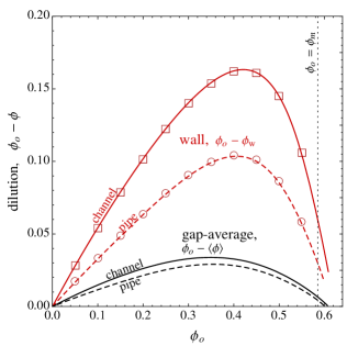
Figure 5: Dilution: change of the wall $\phi_{\text{w}}$ and the gap-average $\left\langle\phi\right\rangle$ values of the solid volume fraction from its entrance value $\phi_{o}$, in the fully-developed channel (solid lines) and pipe (dashed lines) flow. The symbols show the fully-developed limit of the dilution at the wall in the numerical solutions for axial flow development (section 5).

Figure 6 illustrates profiles of the scaled velocity ($v_{x}/\left\langle v_{x}\right\rangle=h/\left\langle h\right\rangle$) and particle concentration, respectively, across the channel for various values of the entrance particle concentration $\phi_{o}$. A transition from Poiseuille to plug flow as the entrance solid volume fraction increases is evident in figure 6, and can be further quantified from the plot of the increasing plug half-width (slot) or radius (pipe) with $\phi_{o}$ in figure 7. The lower limit $\phi_{o}\approx 0.25$ where a flatten velocity profile has been detected experimentally for pipe flow (Cox and Mason, 1971; Hampton et al., 1997) corresponds to a theoretical plug size of about 3% of the pipe radius.

It is also worthwhile to note that the predicted velocity/concentration profiles (based on rheology (15)-(16) proposed in section 2.2) are very similar to the predictions based on original frictional rheology of Boyer et al. (2011a), shown on figure 6 by dashed lines for comparison, as long as $\phi_{o}<0.55$. The main difference between the two models lie in the linear compaction in the central plug allowed for in the former, but not in the latter. The plug compaction starts to impact the velocity profile for value of $\phi_{o}$ close to $\phi_{m}$: the compaction significantly reduces the plug size and allows a higher velocity (see the case $\phi_{o}=0.584$ on figure 6). (In fact, plug compaction allows for fully-developed flows with average concentration exceeding the jamming value, i.e. $\left\langle\phi\right\rangle>\phi_{m}$).

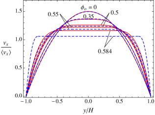
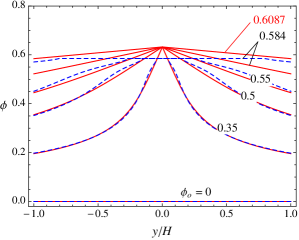
Figure 6: Transition from Poiseuille to plug flow in a channel with increasing entrance solid volume fraction $\phi_{o}$: fully developed velocity profiles scaled by the mean velocity (left) and solid volume fraction profile (right). The results obtained using the frictional rheology with compressible plug (15) are plotted in solid (red) lines whereas the original Boyer et al.’s rheology with an incompressible plug are plotted in dash (blue) lines.

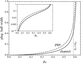
Figure 7: Fully-developed plug half-width (slot, continuous line) and radius (pipe, dashed line) as a function of the entrance solid volume fraction $\phi_{o}$. The inset shows the details of vanishing plug in low solid fraction flows on a semi-logarithmic plot. The plug dimension is scaled by the slot half-width $H$ and pipe radius $R$, respectively.

The evolution of the gap-average tangent fluidity $\left\langle h\right\rangle$ as a function of $\phi_{o}$ is an important quantity to estimate friction pressure in engineering applications. Figure 8 displays the evolution of $\left\langle h\right\rangle$ from the Newtonian limit at $\phi_{o}=0$ to the limit of no flow $\left\langle h\right\rangle=0$ at $\phi_{o}=\left\langle\phi\right\rangle_{\text{plug}}>\phi_{m}$. It is interesting to point out that estimating $\left\langle h\right\rangle$ by directly using the shear viscosity as a function of $\phi_{o}$ in a Newtonian (parabolic) velocity profile results in a poor approximation. Finally, the corresponding evolution of the dimensionless effective normal stress $-\sigma_{n}^{\prime}$ as a function of $\phi_{o}$ is also displayed in figure 8. We can again note that below $\phi_{o}\approx 0.25$, the effective stress appears negligible ($-\sigma_{n}^{\prime}{\normalcolor<0.25}$) in line with experimental observations of Deboeuf et al. (2009); Garland et al. (2013), but it is seen to drastically increase for $\phi_{o}>0.5$.

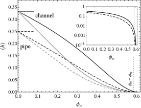
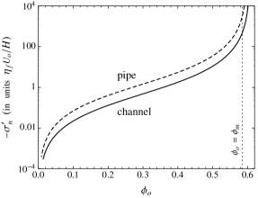
Figure 8: Tangent gap-averaged “fluidity” $\left\langle h\right\rangle$ = the inverse of the mean stress gradient $1/|\nabla p|^{\text{SLOT}}$ or $2/|\nabla p|^{\text{PIPE}}$, when expressed in units of $\eta_{f}U_{o}/H^{2}$ or $\eta_{f}U_{o}/R^{2}$, (left), and effective normal stress $-\sigma_{n}^{\prime}$ in units of $\eta_{f}U_{o}/H$ or $\eta_{f}U_{o}/R$ (right) for fully-developed flow in a slot (solid line) and a pipe (long dash line) as a function of the entrance solid volume fraction $\phi_{o}$. The limiting Newtonian values $1/3$ (slot), $1/4$ (pipe) of $\left\langle h\right\rangle$ for $\phi_{o}=0$ are highlighted, while the inset displays the behavior of $\left\langle h\right\rangle$ in semi-log in the region close to $\phi_{m}$. The approximations $\left\langle h\right\rangle\approx\frac{1}{3\eta_{s}(\phi_{o})}$ (slot), $\frac{1}{4\eta_{s}(\phi_{o})}$ (pipe) obtained by directly taking the relative shear viscosity in a Newtonian parabolic profile are also displayed (light gray continuous and dash lines).

4.5 Comparison with experiments

We now compare the solution for fully developed flow of suspensions governed by a frictional rheology to experimental results available in the literature for low Reynolds number flows of neutrally buoyant, mono-dispersed suspensions in channels and pipes. As previously in figures 5-8, and for the remainder of this paper, we make use of frictional rheology (15)-(16) with parameters $\phi_{m}=0.585$, $\mu_{1}=0.3$, and $\beta=0.158$, which values were determined from matching with rheological measurements of Boyer et al. (2011a) and Dbouk et al. (2013b) (see figure 2). We therefore emphasize that no attempts are taken to “tune” the rheological parameters to the pressure-driven flow experiments data used in the comparisons.

4.5.1 Channel flow

Lyon and Leal (1998a, b) report a series of pressure driven flow experiments at low Reynolds number in a channel on suspensions of mono-disperse PMMA spheres ($2a=70\pm 6$ $\mu$m or $95\pm 12$ $\mu$m) in a Triton X-100/ 1,6-dibromohexane / UCON 75-H oil mixture ($\eta_{f}=4.8\mbox{ Poise})$. Laser Doppler Velocimetry (LDV) was used to image both the velocity and solid volume fraction profiles across the channel gap at a distance sufficiently far from the inlet, where the flow can be considered nearly fully-developed (see Lyon and Leal (1998a) for discussion, and our estimates of the degree of the flow development in Table 1). Tracer-particles optical microscopy was used in some of the experiments (Lyon and Leal, 1998b) and provided better local solid volume fraction measurements compared to those made with the LDV. In particular, the LDV measurements of the solid volume fraction appear to be inaccurate in the outer 20% of the gap due to the channel wall effects (Lyon and Leal, 1998b). When presenting these measurements in figures 9-11, we will show the wall-biased LDV data by a shade of gray to differentiate from higher-confidence measurements in the core of the flow.

Exp. #	$\phi_{o}$	$U_{o}$	$Re_{p}$	$2H$	$2a$	$H/a$	$\left[x/H\right]_{\text{exp}}$	$[L_{\phi}/H]$	development
	-	[mm/s]	[$10^{-6}$]	[mm]	[microns]	-	-	-	%
562 $(\blacktriangle,\vartriangle)$	0.3	4.7	3.6	1.7	95	18	224	415	81
482 $(\blacktriangle,\vartriangle)$	0.4	4.7	1.5	1.7	70	24	280	450	86
483 $(\scalebox{1.3}{$\circ$})$		9.1	2.9	1.7	70	24	280	450	86
553 $(\scalebox{0.75}{$\square$})$		4.7	3.6	1.7	95	18	224	244	94
550 $(\vartriangle)$	0.5	5.4	12.	1	95	11	380	26	100
551 $(\scalebox{1.3}{$\diamond$})$		4.7	3.6	1.7	95	18	224	75
575 $(\scalebox{1.3}{$\circ$})$		5.4	4.9	1	70	14	380	48
008 $(\scalebox{0.75}{$\square$})$		4.7	1.4	1.7	70	24	220	137

Table 1: Summary of the channel flow experiments of Lyon and Leal (1998a, b): $\phi_{o}$ is the entrance solid volume fraction, $U_{o}$ the entrance velocity (computed from the reported flow rate and slot dimensions of $2H$ by 2 inches). $Re_{p}=\frac{4}{3}\frac{\rho}{\eta_{f}}\frac{a^{3}}{H^{2}}V_{max}$ is the particle Reynolds number. The carrier fluid and particles are density matched ($\rho=1190$$\mbox{kg}/\mbox{m}^{3}$), and $\eta_{f}=4.8\mbox{ Poise}$. The last three columns show the axial distance of the measurements from the flow entrance ($x_{\text{exp}}$), the axial distance $L_{\phi}$ at which the flow is predicted to be 95% developed, and the predicted actual percent of flow development at $x_{\text{exp}}$ (based on the numerical solution for axial flow development of Section 5).

Experiments	$\phi_{o}$	$\left\langle\phi\right\rangle$		$\phi_{\text{{w}}}$	$\mu_{\mathrm{w}}$	$-\sigma_{n}^{\prime}$ [Pa]	$-\partial_{x}p$ [kPa/m]
#		Measured	Theory	Theory
562 $(\blacktriangle,\vartriangle)$	0.3	0.28${}^{\text{a}}$	0.267	0.160	11.6	1.27	17.4
		0.24
482 $(\blacktriangle,\vartriangle)$	0.4	0.38${}^{\text{a}}$	0.367	0.238	5.04	4.72	28.0
		0.35
483 $(\scalebox{1.3}{$\circ$})$		0.32				9.13	54.1
553 $(\scalebox{0.75}{$\square$})$		0.36				4.72	28.0
550 $(\vartriangle)$	0.5	0.41	0.477	0.355	2.17	56.3	244
551 $(\scalebox{1.3}{$\diamond$})$		0.42				29.0	73.9
575 $(\scalebox{1.3}{$\circ$})$		0.43				56.3	244
008 $(\scalebox{0.75}{$\square$})$		0.42				29.0	73.9

Table 2: Gap-averaged solid volume fraction $\left\langle\phi\right\rangle$ in the channel flow experiments (Table 1) measured using the LDV (Lyon and Leal, 1998a) and tracer (${}^{\text{a}}$, $\blacktriangle$) particle (Lyon and Leal, 1998b) methods, and its theoretical prediction. (Underestimation of $\left\langle\phi\right\rangle$ when using the LDV method compared to the tracer-particle and theoretically predicted values is due to the poor resolution of the LDV method near the channel walls). Theoretical values of the solid volume fraction $\phi_{\text{w}}$ and friction $\mu_{\text{w}}$ at the walls in the fully-developed flow, measured and theoretical estimate of the normalized velocity width-average. Different set of experiments for similar injected volume fraction $\phi_{o}$.

Table 1 summarizes different experimental conditions tested by Lyon and Leal (1998a), which included tests at different values of the entrance solid volume fraction, particle size, flow rate, and channel width. Table 2 lists values of the mean solid volume fraction across the gap obtained from the reported experimental profiles (by trapezoidal integration) for each series of experiments, as well as the predicted theoretical values accounting for dilution. The experimental values of $\left\langle\phi\right\rangle$ obtained by LDV all appear smaller than the predicted theoretical values, whereas a good match is obtained for the cases where $\phi$ was measured using the tracer particle method. As discussed in Lyon and Leal (1998b), poor resolution of particles by the LDV technique close to the channel walls explains the observed differences of the $\left\langle\phi\right\rangle$-values. In addition, Table 2 lists theoretical predictions for other essential parameters describing the flow for different experiments series, such as wall values of the stress ratio and solid volume fraction (the latter parametrizes the normalized solution for fully-developed flow), the particle normal stress, and the total pressure gradient.

The velocity profiles reported by Lyon and Leal (1998b) were scaled by the maximum (centerline) velocity for a Newtonian flow profile with an identical flow rate (i.e. $V_{max}=3/2\left\langle v_{x}\right\rangle$). The theoretical prediction follows in the form of:

$$\frac{v_{x}}{V_{max}}=\frac{2}{3}\frac{h(\phi(y))}{\left\langle h\right\rangle}$$

where $\phi(y)$, $h(\phi)$, and $\left\langle h\right\rangle$ are given in sections 4.1 and 4.2 as functions of a single parameter, $\phi_{\text{w}}$ or $\mu_{\text{w}}=\mu(\phi_{\text{w}})$. The latter is a unique function of the entrance concentration $\phi_{o}$ given by (43-44), and plotted in figure 5.

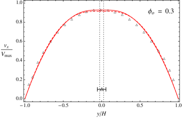
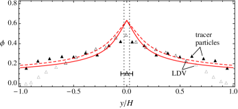
Figure 9: Comparison of the theoretical predictions (solid lines) with the experiment of Lyon and Leal (1998a, b) (Table 1) for channel flow of a suspension with $\phi_{o}=0.3$: scaled velocity profile (top), solid volume fraction profile measured using the LDV $(\vartriangle)$ and tracer-particles $(\blacktriangle)$ methods (bottom). (The solid volume fraction measurements with LDV in the outer 20% of the channel are biased by wall-effects, and are shown in faint gray). Bar shows scaled particle diameter. Predicted diluted gap-averaged particle concentration is $\left\langle\phi\right\rangle\approx 0.267$ (Table 2). Theoretical profiles which neglect dilution, i.e. assume $\left\langle\phi\right\rangle=0.3$, are also shown by dashed lines.

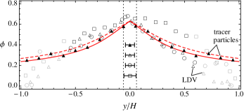
Figure 10: As in figure 9 but for $\phi_{o}=0.4$ (predicted diluted $\left\langle\phi\right\rangle=0.367$).

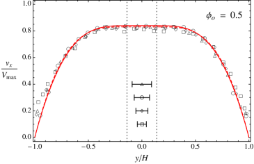
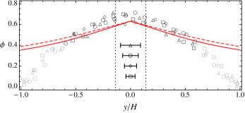
Figure 11: As in figure 9 but for $\phi_{o}=0.5$ (predicted diluted $\left\langle\phi\right\rangle=0.477$).

Figures 9, 10, and 11 display the comparison between the experimental and theoretical profiles of the scaled velocity and the solid volume fraction for $\phi_{o}=0.3$, $0.4$, and $0.5$, respectively. The profiles predicted assuming zero dilution (i.e. $\left\langle\phi\right\rangle=\phi_{o}$) are also shown for comparison (dashed lines). Particle sizes used in various experiments are also shown.

The experimental and theoretical velocity profiles agree very well for all three entrance solid volume fractions tested: the predictions are actually within the experimental measurements error. The frictional suspension rheology is notably able to correctly predict the development of the plug region at the channel centerline as the entrance solid volume fraction increases (see dotted lines marking the predicted plug boundaries).

Examination of the solid volume fraction profiles show a striking overall agreement between the theory and experiment, when the optical particle-tracking method was used to measure $\phi$ (see $\blacktriangle$-symbols in figures 9 and 10 for $\phi_{o}=0.3$ and 0.4, respectively). The discrepancy near the center of the channel for the case with $\phi_{o}=0.3$ stems from the loss of the continuum approximation there, as the particle size in this experiment is about twice the predicted size of the central plug (figure 9). Remarkably, examination of the case with $\phi_{o}=0.4$, where the experimental $\phi$-profile (obtained using optical particle-tracking method) is matched by the theoretical profile everywhere in the gap, including the central plug region, which predicted width spans only about one particle diameter. In the other words, it appears that the continuum approximation for this type of flow holds down to the scale of a single particle.

Comparison to the LDV measured $\phi$-profiles shows expected discrepancy in the outer (adjacent to the wall) region of the flow, due to the previously discussed limitations of the LDV method there. Away from the walls, LDV $\phi$-profiles, although more scattered than the tracer-particle profiles, are in a reasonable agreement with the theory. The most notable deviation from the theoretical $\phi$-profile is observed in the core of the flow with $\phi_{o}=0.5$ (figure 11), where high experimental values of the particle concentration (for some measurements, exceeding the random-close-packing value) may be indicative of partial crystallization in the mono-dispersed suspension.

4.5.2 Pipe Flow

Experimental investigations of suspension flow in a pipe have been performed by Karnis et al. (1966); Cox and Mason (1971); Sinton and Chow (1991) among others. Here, we focus on the results obtained by Hampton et al. (1997) using Nuclear Magnetic Resonance (NMR) method. They conducted measurements in the flow of mono-dispersed ($2a=3175$ $\mu$m) and slightly polydispersed ($650\pm 110$ $\mu$m) suspensions of PMMA spheres in pipes with internal diameter $2R=50.8$ mm and $25.4$ mm, respectively, at various values of the entrance solid volume fraction. Tested particle-to-pipe radius ratios were $a/R=1/16$ and $1/39$, respectively. The liquid solution of UCON oil (H-9500), polyalkylene glycol and tetrabomoethane with a reported viscosity of $2.1$ Pa$\cdot$s was used as the carrying fluid.

$\phi_{o}$	$\left\langle\phi\right\rangle$		$\phi_{\text{{w}}}$	$\mu_{\mathrm{w}}$	$-\sigma_{n}^{\prime}$ [Pa]	$-\partial_{x}p$ [kPa/m]
	Measured	Theory	Theory
0.2	0.17${}^{\text{a}}$	0.179	0.137	16.1	6.6	16.7
	0.16${}^{\text{b}}$				3.3	4.2
0.3	0.27${}^{\text{a}}$	0.272	0.210	6.51	24	24.5
	0.25${}^{\text{b}}$				12	6.1
0.45	0.41${}^{\text{a}}$	0.425	0.350	2.24	90	71
	0.41${}^{\text{b}}$				45	17.7

Table 3: Gap-averaged solid volume fraction $\left\langle\phi\right\rangle$ in the pipe flow experiments measured using the NMR method (Hampton et al., 1997), and the corresponding theoretical prediction (independent of particle size). The two different sets of experimental conditions correspond to (${}^{\text{a}}$) $2R=25.4$ mm, $a/R=1/39$; and (${}^{\text{b}}$) $2R=50.8$ mm, $a/R=1/16$. We also give theoretical predictions of the solid volume fraction and the stress ratio at the pipe wall, as well as the particle normal stress and the total pressure gradient for an assumed value of the average flow velocity ($U_{o}=100$ mm/s).

Velocity and solid volume fraction profiles for three different values of the entrance solid volume fraction ($\phi_{o}=0.2,\,0.3$, and $0.45$) are compared in figure 12 to the theoretical predictions based on the frictional rheology. Scaled radii of small and large particles are also indicated.

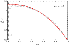
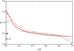
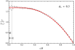
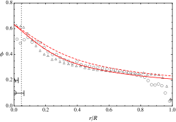
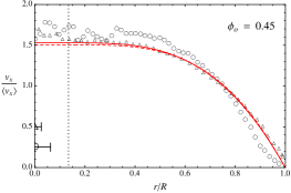
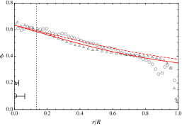
Figure 12: Comparison of the theoretical predictions (solid lines) of the scaled velocity (left) and solid volume fraction (right) profiles with experiments of Hampton et al. (1997) for pipe flow of suspensions with $\phi_{o}=0.2$ (top), $\phi_{o}=0.3$ (middle), and $\phi_{o}=0.45$ (bottom) and two different particle-to-pipe radius ratios, $a/R$ = $1/39\,(\vartriangle)$ and $1/16$ ($\circ$). Bars show scaled values of the particle radius in the experiments. Dotted lines show the predicted plug boundary. Theoretical values of the diluted, gap-averaged particle concentration are $\left\langle\phi\right\rangle=0.179$, 0.272, and 0.425 for $\phi_{o}=0.2$, 0.3, and 0.45, respectively (Table 3). Theoretical predictions which neglect dilution are also shown (dashed lines) for comparison.

Similar to the comparisons drawn for channel flow in the preceding section, the theoretical velocity profiles for pipe flow are in excellent agreement with the experimental results, especially so for the suspensions with the smaller particle size ($\vartriangle$). The only notable discrepancy between experimental and theoretical velocity profiles is observed for the suspension with the larger particle size ($\circ$) at the highest solid volume fraction ($\phi_{o}=0.45$) studied experimentally. This may have resulted from partial crystallization of the mono-dispersed suspension in the high concentration flow (as measured $\phi$-values in this case slightly exceed the theoretical ones in the bulk of the flow, see bottom plot of figure 12).

The experimental solid volume fraction profiles compare well with the theoretically predicted ones with the exception of a particle-size boundary layer at the pipe’s wall, where experimental values are lower. Gap-averaging of the fully-developed experimental profiles indicates dilution from the corresponding entrance values, and compares well to the predicted values of $\left\langle\phi\right\rangle$ (Table 3).

Similarly to our observations for channel flow, measured $\phi$-values near the axis of the pipe agree very well with the predicted values when the (predicted) plug diameter exceeds the particle size, $r_{plug}>a$, (see the cases with the smaller particle size for $\phi_{o}=0.2$ and $\phi_{o}=0.3$, and the case with either large or small particles for $\phi_{o}=0.45$, figure 12). When the predicted plug size is smaller than the particle size ($r_{plug}<a$), the experimental $\phi$-profile is flattened (compared to the theoretical prediction) over a particle-sized region which embeds the predicted plug (see the cases with the larger particles size for $\phi_{o}=0.2$ and $\phi_{o}=0.3$, figure 12).

It is also interesting to observe an approximate linearity of the solid volume fraction profile within the central plug when the latter is resolved on a particle scale ($r_{plug}>a$), e.g. for all cases with the smaller particles (figure 12). Such a linear compaction is captured by the proposed rheology, which extends the linear relation between the solid volume fraction and the stress ratio from the dense flowing regime into the fully-jammed state.

5 Axial flow development

We now examine the axial development of the flow from the inlet of the channel toward its fully-developed state.

5.1 Numerical Solution

Setting $\delta=a/H$ to zero, the solid continuity equation (27) together with the expression for the cross-component of the relative flux (26) become

$$\frac{1}{\phi}\frac{d\phi}{dt}=\frac{\partial q_{y}}{\partial y},\qquad q_{y}{\normalcolor=-\kappa(\phi)\frac{\partial\sigma^{\prime}_{yy}}{\partial y}}$$ (45)

where $d/dt=v_{x}\partial/\partial x+v_{y}\partial/\partial y$ for a steady flow ($\partial/\partial t=0$). The solid volume change can be related to that of the stress ratio $\mu=-\tau/\sigma_{n}^{\prime}$ via the inelastic “compressibility” $d\phi/d\mu$, defined by a unique function of the stress ratio across jammed ($0<\mu<\mu_{1}$) and flowing ($\mu>\mu_{1}$) states of the suspension (figure 4). This leads to a specialization of (45), which can be viewed as a non-linear consolidation equation in terms of the particle normal stress $\sigma^{\prime}_{n}$,

$$\frac{S(\phi)}{\sigma^{\prime}_{n}}\frac{d\sigma^{\prime}_{n}}{dt}-\frac{S(\phi)}{\tau}\frac{d\tau}{dt}=\frac{\partial q_{y}}{\partial y},\qquad q_{y}=-\kappa(\phi)\frac{\partial\sigma^{\prime}_{n}}{\partial y},$$ (46)

where

$$S(\phi)=-\frac{\mu}{\phi}\frac{\mbox{d}\phi}{\mbox{d}\mu}>0$$ (47)

is the inelastic storage coefficient.

The reduced ($\delta=0$) form of the mixture continuity equation (28) is:

$$\frac{\partial v_{x}}{\partial x}+\frac{\partial(v_{y}+q_{y})}{\partial y}=0$$ (48)

Continuity equations (46-48), momentum balance, $\tau=|\nabla p|y$ (equation (32)), and the expression

$$\frac{\partial v_{x}}{\partial y}=\sigma_{n}^{\prime}\,\mathcal{I}(-\tau/\sigma_{n}^{\prime}),$$ (49)

where $\mathcal{I}(\mu)$ is the rheological dependence of $I(\phi)$ (equation (16)) on $\mu(\phi)$ (equation (15)), are solved numerically together with the boundary conditions (29-30) for the axial development of the unknown particle normal stress $\sigma_{n}^{\prime}(x,y)$, particle velocity components $v_{x}(x,y)$ and $v_{y}(x,y)$, and the total pressure gradient $|\nabla p(x)|$ with $x\geq 0$ and $0\leq y\leq 1$ (using the channel symmetry).

We start with formulating the entrance conditions ($x=0$) for the unknowns. For a uniform particle concentration profile at the flow entrance, $\phi(x=0,y)=\phi_{o}$, we have for the particle stress and velocity there

$${\normalcolor-\sigma_{n}^{\prime}=\frac{\left|\nabla p_{o}\right|y}{\mu_{o}},\quad}v_{x}=-\int_{y}^{1}\sigma_{n}^{\prime}I_{o}dy=\left|\nabla p_{o}\right|\frac{I_{o}}{\mu_{o}}\frac{1-y^{2}}{2}\quad\text{at}\quad x=0,$$ (50)

respectively, where $\mu_{o}=\mu(\phi_{o})$ and $I_{o}=I(\phi_{o})$ are the corresponding rheological values of $\mu$ and $I$. Given the gap-average value $v_{o}=1$ of the entrance velocity, we find the entrance value of the mean stress gradient to be

$$\left|\nabla p_{o}\right|=\frac{3\mu_{o}}{I_{o}}$$ (51)

We adopt the following iterative approach to the numerical solution.

• At the start (the zeroth iteration), all unknowns are assigned to their entrance values (50-51), i.e. $v_{x}^{(0)}(x,y)\equiv v_{x}(x=0,y)$, $\sigma_{n}^{\prime(0)}(x,y)\equiv\sigma_{n}^{\prime}(x=0,y)$, etc, except for the mean stress gradient, which initial guess is assigned to vary smoothly along the channel from the entrance value $\left|\nabla p_{o}\right|$, (51), to the fully-developed value $\left|\nabla p_{\infty}\right|=1/\left\langle h\right\rangle$ (Section 4) at the end $x=x_{\text{end}}$ of the computational interval. The latter is chosen to be a finite multiple of our estimate of the flow development length, as discussed below in Section 5.3. The partial differential equation (46) is then solved for the 1st iteration of the particle stress, $\sigma_{n}^{\prime(1)}(x,y)$, using the method of lines PDE solver (Mathematica, ver. 9). Corresponding numerical error can be assessed from contrasting the left and right hand sides of the consolidation equation (46), which can be evaluated from the obtained solution at various channel cross-sections (see figure 1 of the supplementary materials). The error is generally not discernible across the entire channel width with the exception of a one discretization step thick ($\sim 0.01$ for solutions reported here) region at the channel center.

• The 1st iteration of the mean stress gradient, $|\nabla p^{(1)}(x)|$, is then found from applying the global continuity condition $\left\langle v_{x}\right\rangle=1$, where the gap-averaged velocity can be evaluated with the help of (49) as

  $$\left\langle v_{x}\right\rangle=-\int_{0}^{1}\sigma_{n}^{\prime}\,\mathcal{I}\left(\frac{|\nabla p|\,y}{-\sigma_{n}^{\prime}}\right)y\,\text{d}y$$ (52)

  In order to solve the resulting integral equation for $|\nabla p|$ we use a sub-iterative procedure

  $$|\nabla p_{\text{(next)}}|=\frac{1}{\left\langle v_{x}\right\rangle_{\text{(prev.)}}}|{\normalcolor\nabla p_{\text{(prev.)}}|}$$ (53)

  where “next” and “prev.” refer to successive sub-iterations on $|\nabla p|$, and $\left\langle v_{x}\right\rangle_{\text{(prev.)}}$ is given by (52) evaluated at $|\nabla p|=|\nabla p_{\text{(prev.)}}|$.

• Once $|\nabla p^{(1)}|$, $\tau^{(1)}=|\nabla p^{(1)}{|}y$ and $\mu^{(1)}=-\tau^{(1)}/\sigma_{n}^{\prime}$ are at hand, we recover the 1st iterations of the particle concentration, $\phi^{(1)}(x,y)$ from the rheological relations (15)-(16), and of the axial velocity $v_{x}^{(1)}(x,y)$ (by integrating (49)), respectively. The 1st iteration of the cross-velocity $v_{y}^{(1)}(x,y)$ follows from integrating in $y$ the mixture continuity (48), where the relative cross-flux is given by $q_{y}^{(1)}=-\kappa(\phi^{(1)})(\partial\sigma_{n}^{\prime(1)}/\partial y)$.

The above three steps are repeated until the iterations converge. We assess the convergence using the gap-average of the particle concentration in the fully-developed part of the flow (at large enough distances $x$ from the entrance), specifically requiring $|\left\langle\phi\right\rangle^{(i)}-\left\langle\phi\right\rangle^{(i-1)}|<10^{-4}\times\phi_{o}$ to stop the iterations. We found that using a weighted average between the last two iterations (e.g., $0.75v_{x}^{(i-1)}+0.25v_{x}^{(i-2)}$) to compute the next ($i\mbox{th}$) iteration improves the iterations stability and convergence rate. Similarly, in sub-iterative procedure of step 2, we have settled on a similar “weighted” modification of (53). We found a typical number of iterations required for the convergence to vary from the minimum of 2 to the maximum of 12-14, with larger numbers corresponding to larger values of the entrance concentration.

The described numerical method is readily transportable to pipe flow. In the following, we therefore present results pertaining to both channel and pipe flow development.

5.2 Examples

As stipulated earlier, we use the constitutive rheology (15)-(16) with parameters $\phi_{m}=0.585$, $\mu_{1}=0.3$, and $\beta=0.158$, and Richardson-Zaki expression for the flow hindrance function with laboratory-determined exponent $\alpha=5.1$ (i.e. $f(\phi)=(1-\phi)^{5.1})$. Corresponding numerical solutions for axial development of the solid volume fraction $\phi$ and the particle normal stress $-\sigma_{n}^{\prime}$ in a channel and a pipe are visualized on figures 13 and 14, respectively, for three different values of the entrance particle concentration ($\phi_{o}=0.3,$ 0.4, and 0.5). Corresponding profiles of $v_{x}$, $\phi$, and $-\sigma_{n}^{\prime}$ in a number of flow cross-sections ($x=10^{-3},$ 0.01, 0.1, and 1) are shown on figures 2, 3, and 4 of the supplementary materials.

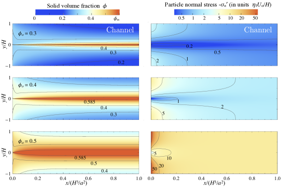
Figure 13: Development of the flow in a channel of half-width $H$ for three different entrance values of the solid volume fraction, $\phi_{o}=0.3,0.4,$ and $0.5$. (left) Evolution of the solid volume fraction. (right) Evolution of the particle normal stress $-\sigma_{n}^{\prime}$ in units of $\eta_{f}U_{o}/H$.

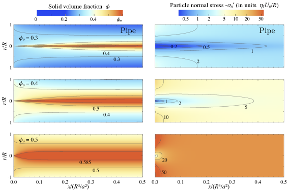
Figure 14: Development of the flow in a pipe of radius $R$ for three different entrance values of the solid volume fraction, as in figure 13 for channel flow.

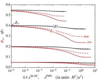
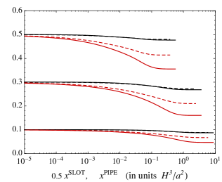
Figure 15: Development of the wall and gap-average values of the solid volume fraction with axial distance from the entrance in the channel (solid line) or pipe (dashed line) flow. Distance $x$ is in units of ($H^{3}/a^{2}$ or $R^{3}/a^{2}$), and $x^{\text{SLOT}}$ is scaled by prefactor 1/2. It is evident that the particle concentration in the pipe flow with radius $R$ develops approximately twice as fast as it does in the slot with half width $H=R$ for identical particle size $a$. Results are for values of entrance concentration $\phi_{o}=$0.05, 0.2, 0.4, 0.55 (left) and $\phi_{o}=$0.1, 0.3, 0.5 (right), corresponding to the intercepts with the $\phi$- axis.

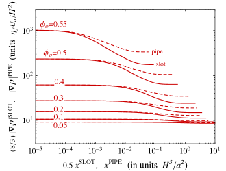
Figure 16: Development of the total pressure gradient in units of $\eta_{f}U_{o}/H^{2}$ or $\eta_{f}U_{o}/R^{2}$ with axial distance from the entrance in the channel (solid line) or pipe (dashed line) flow. The total pressure gradient in the channel $|\nabla p|^{\text{SLOT}}$ is scaled by prefactor $8/3$, such that $(8/3)|\nabla p|^{\text{SLOT}}=|\nabla p|^{\text{PIPE}}$ at the channel/pipe entrance when $H=R$. Distance $x$ is in units of $H^{3}/a^{2}$ or $R^{3}/a^{2}$, and $x^{\text{SLOT}}$ is scaled by prefactor 1/2.

Figure 15 shows development of the solid volume fraction, the gap-averaged and wall values thereof, for various entrance conditions, and figure 16 shows similar development of the mixture pressure gradient driving the suspension flow. Flow in a pipe is seen to develop significantly faster than flow in a channel of equivalent half-width (i.e. with $H=R$). This observation is further quantified below.

5.3 Development length

We expect the normalized axial flow development length to scale with the gap-averaged normalized axial velocity ($v_{o}=1$) divided by the normalized diffusivity coefficient $D$ (equation (46)), e.g.,

$$L_{\text{dev}}=\frac{1}{4\left\langle D\right\rangle},\qquad D=\frac{{(-\sigma_{n}^{\prime})}\kappa(\phi)}{S(\phi)}$$

To specialize the latter, we choose to evaluate $\left\langle D\right\rangle$ at the channel entrance, where solid volume fraction is uniform and the corresponding expressions for the particle normal stress and the axial velocity are given by (50) and (51), yielding the normalized development lengthscale expression

$$L_{\text{dev}}=\frac{1}{6}\frac{I(\phi_{o})S(\phi_{o})}{\kappa(\phi_{o})}$$ (54)

in terms of the normalized permeability $\kappa(\phi)=2f(\phi)/9\phi$, inelastic storage coefficient $S(\phi)=-(\mu/\phi)(\mbox{d}\phi/\mbox{d}\mu)$ (equation (47)), and the viscous number $I(\phi)$.

Corresponding dimensional diffusivity and development lengthscale can be readily recovered from the normalized expressions above using units $H^{2}/t_{*}=U_{o}H^{3}/a^{2}$ (diffusivity), $\tau_{*}=\eta_{f}U_{o}/H$ (mean particle stress), and $L=H^{3}/a^{2}$ (axial length), (equations (18-22)):

$$L_{\text{dev}}=U_{o}\frac{H^{2}}{4\left\langle D\right\rangle_{o}}=\frac{H^{3}}{a^{2}}\frac{I(\phi_{o})S(\phi_{o})}{6\,\kappa(\phi_{o})},\qquad D=\frac{a^{2}\kappa(\phi)}{\eta_{f}}\frac{(-\sigma_{n}^{\prime})}{S(\phi)}$$ (55)

To track flow development, we make use of a measure (Hampton et al., 1997)

$$E_{p}(x)=\left\langle\left|\phi(x,y)-\phi_{o}\right|\right\rangle/\phi_{o}$$ (56)

of the non-uniformity of the solid volume fraction profile, which varies from zero at the flow entrance to the maximum, fully-developed value away from the entrance. Figure 17 contrasts Hampton et al.’s measurements of $E_{p}$ for a suspension system with $\phi_{o}=0.45$ at various stages of the flow development to our numerical predictions for Richardson-Zaki ($\alpha=5.1$) permeability. The match between the theory and the experiment is remarkable, in that no constitutive parameters have been adjusted from their values, as determined from independent sets of rheological experiments.

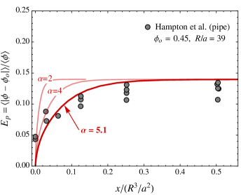
Figure 17: Numerical predictions for the evolution of number $E_{p}$ quantifying the non-uniformity of solid volume fraction profile (maximum $E_{p}$ corresponds to the fully-developed flow) for $\phi_{o}=0.45$, contrasted with the experimental data of Hampton et al. (1997) for the system with $a/R=1/39$. The solid line corresponds to the predictions for the Richardson-Zaki permeability function with exponent $\alpha=5.1$ derived from numerous independent sedimentation experiments (see figure 1, and Garside and Al-Dibouni (1977); Davis and Acrivos (1985)), while opaque lines show predictions for other values of $\alpha$ used in the previous numerical modeling of suspension flow development.

Now we seek a similar comparison for the development length. Following Hampton et al. (1997) (see also Miller and Morris (2006)), we define the 95% development length, $L_{\phi}$, for the particle concentration profile as the minimum distance from the flow entrance where $E_{p}$ is within 5% of its fully-developed value. We show on figure 18a that, for Richardson-Zaki ($\alpha=5.1$) permeability, the numerical solutions for the entire range of solid volume fraction are well approximated by

$$L_{\phi}^{\text{pipe}}\approx 0.5\times L_{\phi}^{\text{slot}}\approx 1.136\,L_{\text{dev}}$$

with $L_{dev}$ given by (55) in which $R$ replaces $H$ for the case of a pipe. Hampton et al.’s development data for pipe flow for the system with a smaller particle size (filled circles) is in excellent agreement with numerical model predictions. The experimentally observed development length for suspensions of large particles (filled triangles) deviates upward of the theoretical prediction whenever the predicted central plug width is smaller than the particle size (see figure 12 for comparison of predicted values of plug width to a particle size), or, in other words, when the continuity approximation fails on the scale of the plug.

Figure 18b reproduces the results of figure 18a but in semi-log scale, which allows to better track vanishing development length in the dense regime, when the entrance concentration $\phi_{0}$ approaches its maximum flowing value. Development length predictions for other values of Richardson-Zaki exponent ($\alpha=2$ and $\alpha=4$), as used in some previous studies of suspension flow (Morris and Boulay, 1999; Miller and Morris, 2006), are also shown on figure 18b for comparison. For example, the predicted development length based on an artificially-high permeability with $\alpha=2$ is only a small fraction $\approx(1-\phi)^{3.1}$ of the development length based on the experimentally-validated permeability with $\alpha=5.1$. The underestimation by the former is particularly severe in the dense regime, e.g. by factor of $\approx 9$ for $\phi_{o}=0.5$.

Examination of similarly defined 95% development length $L_{\nabla p}$ for the driving total pressure gradient (shown as a fraction of $L_{\phi}$ on figure 19) suggests that the total pressure gradient develops somewhat faster than the concentration profile, consistent with the previous prediction with suspension balance models (e.g. Miller and Morris, 2006).

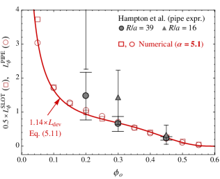
(a) (b)

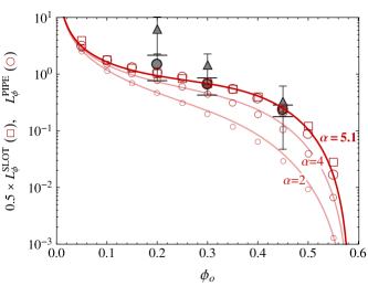
Figure 18: (a) Development length for the particle concentration profile, $L_{\phi}$ in units of ($H^{3}/a^{2}$ or $R^{3}/a^{2}$), as a function of entrance particle concentration $\phi_{o}$. (Richardson-Zaki exponent $\alpha=5.1$.) The development length for the pipe flow is approximately half of that for the slot flow. The open symbols show the numerical solutions, and the solid line shows an approximation based on the apparent diffusivity, $L_{\phi}^{\text{pipe}}\approx 0.5\times L_{\phi}^{\text{slot}}\approx 1.136\,L_{dev}(\phi_{o})$ (equation (54)). The filled circles and triangles show the data of Hampton et al. (1997) for two systems, with smaller $R/a\approx 39$ and larger $R/a\approx 16$ particles, respectively. (b) Same as (a) but in log-linear scale, to examine vanishing development length in the limit of large solid volume fraction. Development length of the numerical solutions for pipe flow characterized by other (than $\alpha=5.1$) values of Richardson-Zaki exponent and corresponding approximation using equation (54) are also shown by small open circles and opaque lines, respectively.

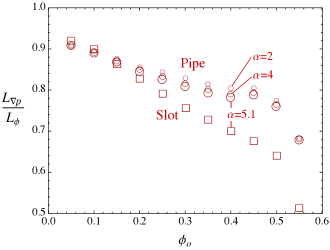
Figure 19: The ratio $L_{\nabla p}/L_{\phi}$ of the total pressure gradient development length and the SVF development length, respectively, as a function of entrance SVF $\phi_{o}$.

6 Discussion

The theoretical predictions for the fully-developed flow based on the frictional suspension rheology are in excellent agreement with the experimentally measured fully-developed velocity and volume fraction profiles for both pipe and channel geometries (Lyon and Leal, 1998a; Hampton et al., 1997). In particular, the radius / half-width of the central plug is very well predicted in all cases. These predictions of the experimental responses are to be compared with the ones obtained on the same set of experimental data using suspension balance models. Among those, Miller and Morris (2006) and Fang et al. (2002) predict no discernible plug, which is likely due to an unrealistically large (in excess of the random close packing limit) value of $\phi_{m}$ assumed in these studies. A finite plug, albeit still of a smaller size than that observed in the experiments of Hampton et al. (1997), is predicted from suspension balance modeling by Ramachandran (2013), who used a more plausible (below the random close packing limit) value of $\phi_{m}$.

Another interesting point that arises from the comparisons of the predicted and experimentally observed fully-developed profiles relates to the limit of validity of the continuum (macroscopic) assumption. As already mentioned in section 4.5, the experimental solid volume fraction in the plug are in agreement with the continuum theory as long as the plug width is larger than at least one particle. Similarly for the case of the pipe flow (imaged by NMR), the predictions of the solid volume fraction close to the wall are in good agreement with experimental values at a distance from the wall larger than one-to-two particles. In other words, the continuum theory can resolve the flow relatively accurately at a scale of a single particle. It is clear that in dilute cases (for low $\phi_{o}$), the size of the plug is eventually getting smaller than the particle size. In this case, one would have, therefore, to introduce the latter as an internal lengthscale in the constitutive description, effectively making it non-local (e.g., Miller and Morris, 2006).

It is worthwhile to recall that all of the experiments investigated here are characterized by a value of the gap width of at least ten particle wide, and by a plug size of at most 20% of the gap width (as in the case of $\phi_{o}=0.5$, see figure 11). From the quality of the agreement obtained between the predictions based on a local rheology and the experiments, we can conclude that non-local effects may not be important in the considered cases. These effects may become important for larger values of the particle-to-gap or/and plug-to-gap ratios, i.e. for bulk concentration values $\phi_{o}$ closer to $\phi_{m}$ than those studied experimentally by Lyon and Leal (1998a) and Hampton et al. (1997). It would be particularly interesting to further test our proposed extension of the frictional rheology to the non-flowing state, in the form of the linear relation between the stress ratio $\mu$ and the solid volume fraction $\phi$, to cases where $\phi_{o}$ is closer to $\phi_{m}$ (e.g., for $\phi_{o}=0.55$ and higher), as well as for larger values of the particle-to-gap ratio.

To our knowledge, we predict for the first time the axial development of the flow (e.g. “entrance” length) and the fully-developed flow measured in pipe and channel experiments (Hampton et al., 1997; Lyon and Leal, 1998a) using a model which is devoid of any fitting parameters. Specifically, this model is completely defined by the normalized permeability $\kappa(\phi)$ (or hindrance $f(\phi)$), friction $\mu(\phi)$, and viscous number $I(\phi)$ functions derived from independent experimental data sets: Garside and Al-Dibouni (1977) and Davis and Acrivos (1985) for the hindrance function, and Boyer et al. (2011a) for frictional rheology. In some previous studies, Miller and Morris (2006) used a suspension-balance model with an artificially large value of the jamming solid volume fraction ($\phi_{m}=0.68$ instead of $\sim 0.6$), artificially low value of the near jamming friction coefficient ($\mu_{1}\approx 0.13$ instead of $\sim 0.3$) and an artificially high permeability (corresponding to the hindrance function of Richardson-Zaki form with an exponent $\alpha=2$ instead of the experimental value $\sim 5$) to solve for axial flow development. The permeability/hindrance function they have used is $1/(1-\phi)^{3}$ times higher than the experimentally measured one. For example, for $\phi=0.45$, this permeability exaggeration factor is $6.$ On the other hand, the inelastic storage factor $d\phi/d\mu$ in their model is also exaggerated. The two exaggerations partially “neutralize” each other in the expression for the diffusivity and therefore in their predicted development length.

7 Conclusions

Using a local continuum formulation based on the frictional constitutive law similar to the one proposed by Boyer et al. (2011a), we have revisited confined, pressure-driven Stokesian suspension flow in a channel and a pipe. We have obtained an analytical solution for the fully developed flow which exhibits the transition from Poiseuille to plug flow with increasing solid concentration, thanks to the particle pressure dependent yield stress of the frictional rheology. The theoretical fully-developed solid volume fraction and velocity profiles agree very well with experimental data available in the literature for these flows without any adjustment of the constitutive parameters obtained from independent rheological experiments in an annular shear cell (Boyer et al., 2011a). Slight mismatches of the solid volume fraction profile are observed when the size of the predicted plug is lower than about one particle diameter, i.e. when the continuum approximation is breaking down in the jammed part of the flow. It is particularly striking that a continuum description can resolve the flow down to the scale of one particle.

A modification of the original constitutive law of Boyer et al. (2011a) has been proposed in order to avoid an unphysical behavior of the plastic compressibility coefficient $\beta=-d\phi/d\mu$ close to the jamming limit. The proposed modification resolves a slight inconsistency in Boyer et al.’s formulation by ensuring the dominance of the contacts over the hydrodynamics contributions to the macroscopic friction in the dense regime. This modification does not affect the fully developed solution (figure 6) to any significant degree for injected volume fraction lower than $0.55$.

We also proposed to extend the linear plastic “compressibility” between the solid volume fraction $\phi$ and the stress ratio $\mu$ into the jammed part of the flow (i.e. when $\phi>\phi_{m}$ and $\mu<\mu_{1}$), and obtained $\phi\approx\phi_{rcp}$ when $\mu\approx 0$. This type of linear compaction in non-flowing regions appears to be present within the central plug in the existing pipe and channel flow experiments. It may be enabled by microscopic velocity and particle pressure fluctuations (similar to tapping or cyclic deformation applied to compacting static granular packs (e.g. Knight et al., 1995; Pouliquen et al., 2003)) originating, in this case, from the surrounding flowing material. This stress-ratio-dependent compaction in the non-flowing part may be linked, by extension, to the dilation property of flowing (sheared) suspensions and dry granular materials, where $\phi$ decreases with the increase in the applied stress ratio $\mu>\mu_{1}$. We conjectured, that this dilation property is preserved in the non-flowing part, where the stress ratio is below the flow threshold ($\mu<\mu_{1}$), if an external energy source, e.g. in the form of velocity/pressure fluctuations originating from the surrounding flowing material, is present in order to facilitate microscopic, “in-cage” particle rearrangements, within the jammed pack. It is worthwhile to note that such an extension of the frictional rheology to the jammed state as well as the solution framework for the fully-developed flow can be directly transferred to the case of a dry, frictional granular media.

The compaction in the plug impacts the suspension velocity for values of the entrance solid volume fraction above $0.55$, allowing flow of denser suspensions with maximum gap-average exceeding the jamming threshold $\phi_{m}$, i.e. $\max\left\langle\phi\right\rangle=(\phi_{m}+\phi_{\mathrm{rcp}})/2$ for the channel and $(2\phi_{m}+\phi_{\mathrm{rcp}})/3$ for the pipe flow.

The axial development of the flow has been solved numerically. The entrance length of the flow in channel and pipe is a function of the fluid permeability / sedimentation hindrance function governing the relative phase slip and of the compressibility coefficient. Our numerical results compare well with existing experimental data for pipe flow when using the accepted values of the parameters of known phenomenological models (e.g., Richardson-Zaki phenomenology). We notably predict that the entrance length is longer for dilute suspensions, and about twice longer in slot compared to pipe flow. Departure from the continuum assumption in experimental flows with larger particles size (which we ascertain to be the case when the predicted plug size is smaller than one particle diameter) is manifested by an increase of the experimentally-observed development length over the prediction. Another mechanism which may potentially contribute to longer-than-predicted development length corresponds to the relaxation / compaction timescale for the jammed plug (which can be related to the number and magnitude of velocity fluctuations required to compact the plug, analogous to the number and magnitude of taps required to relax a static granular pack).

More experimental investigations are needed in order to further test the continuum description of these confined flows. In particular, the case of a higher entrance solid volume fraction $(\phi_{o}>0.55)$ needs to be investigated experimentally in order to further check whether the proposed extension of the plastic compressibility in the jammed state $(\phi>\phi_{m})$ is indeed relevant. Finally, the regime of a larger ratio of the particle size over the channel width, $a/H$, which is relevant for some applications, also needs to be further addressed both experimentally and theoretically.

Acknowledgments

We would like to thank Schlumberger for support to D.G. and for the permission to publish this work.

Appendix A Fully-developed flow in a pipe

A.1 Scaling and normalized solution

There is no particular difficulty in extending the solution for channel flow to the pipe geometry. In particular, the zero-order problem is very similar. We consider a pipe of radius $R$ and characteristic axial length $L$. We are interested in the case where $\delta=R/L$ is small. As before, the coordinates in the $x$ and $r$ direction are scaled with respect to $L$ and $R$ respectively. We assume an axi-symmetric flow independent of the azimuthal position $\theta$. The scaling of the velocity and stress component are similar to that of the channel:

$$t_{*}=\frac{L}{U_{0}}\qquad x_{*}=L\qquad r_{*}=R\qquad(v_{x})_{*}=U_{0}\qquad(v_{r})_{*}=\delta U_{0}\qquad\dot{\gamma}_{*}=\frac{U_{0}}{R}$$ (57)

shear stress ($\tau_{*}$), particle stress ($p_{*}^{\prime}$), fluid pressure ($p_{*}^{f}$), and mixture pressure ($p_{*}$) scale

$$\tau_{*}=p_{*}^{\prime}=\frac{\eta_{f}U_{0}}{R}\qquad p_{*}=p_{*}^{f}=\frac{\tau_{*}}{\delta}$$ (58)

and relative phase flux scale

$$q_{*}\equiv\frac{a^{2}}{\eta_{f}}\frac{p_{*}^{f}}{L}=\left(\frac{a}{R}\right)^{2}U_{0}$$ (59)

It is possible to show that the balance and continuity equations have similar form as in the channel case, accounting for the proper differential operator in polar coordinates and assuming negligible normal stress difference $\sigma_{rr}^{\prime}-\sigma_{\theta\theta}^{\prime}\approx 0$. The latter assumption approximately holds for dilute suspensions, but breaks down for concentrated ones (e.g. Couturier et al., 2011; Zarraga et al., 2000). The fully-developed solution framework developed here can be extended to account for the normal stress difference, and will be pursued elsewhere.

The similar arguments as those for the channel geometry can be made for the axial development length in the pipe flow by looking at the first order terms in $\delta$, which lead to the choice of development lengthscale $L=R^{3}/a^{2}$.

The shear rate is simply $\dot{\gamma}=\left|\partial v_{x}/\partial r\right|$ and the shear stress $\tau=\tau_{xr}$. Following the same method as for the channel flow, we obtain after use of the symmetry and boundary conditions:

$$\tau = \frac{1}{2}\left|\frac{\partial p}{\partial x}\right|r$$

$$p = p(x)\qquad p^{f}=p^{f}(x)$$

In the flowing part, we can write ${\tau/(-\sigma^{\prime}_{n})}=\mu_{\mathrm{w}}r$, where

$$\mu_{\mathrm{w}}=\mu(\phi_{\text{w}})=\frac{1}{2}{\displaystyle{\color[rgb]{0,0,0}\frac{\left|\partial p/\partial x\right|}{{\normalcolor-\sigma^{\prime}_{n}}}}}$$

is the wall friction and $\phi_{\text{w}}$ is the wall value of the solid volume fraction. The friction and solid volume fraction profiles then follow in the form identical to that of the channel:

$$\mu(\phi(r))=\mu_{\mathrm{w}}r$$ (60)

The shear rate can then be expressed as

$$\frac{\partial v_{x}}{\mbox{$\partial$}r}=-\frac{1}{2}\frac{I(\phi(r))}{\mu_{\mathrm{w}}}\times\frac{\partial p}{\partial x}$$

which upon integration using the no-slip condition at the wall yields

$$v_{x}(r)=-\frac{h(\phi(r))}{2}\times\frac{\partial p}{\partial x}$$ (61)

where the function $h(\phi)$ is exactly the same function as for the channel flow (see Eq. (38)).

A.2 Cross-sectional averages

The cross-section averages are slightly different than for channel flow due to the difference in the flow geometry: $\left\langle\cdot\right\rangle=2\int_{0}^{1}(\cdot)r\mbox{ d}r$. The average velocity becomes:

$$\left\langle v_{x}\right\rangle=-\frac{\left\langle h\right\rangle}{2}\times\frac{\partial p}{\partial x}$$

where, similarly to the channel case, integrating separately over the plug and the flowing part, and using substitution $\text{d}r=\text{d}\mu/\mu_{w}$ in the latter, we can obtain

$$\left\langle h\right\rangle=\frac{1}{\mu_{\mathrm{w}}^{4}}\int_{\phi_{m}}^{\phi_{\text{w}}}I(\phi)\,\mu^{2}(\phi)\frac{\mbox{d}\mu}{\mbox{d}\phi}\mbox{ d}\phi$$ (62)

The gap-average of the solid volume fraction is obtained as:

$$\left\langle\phi\right\rangle=\frac{2}{\mu_{\mathrm{w}}^{2}}\int_{\phi_{rcp}}^{\phi_{\mathrm{w}}}\phi\mu(\phi)\frac{\mbox{d}\mu}{\mbox{d}\phi}\mbox{ d}\phi=\frac{\mu_{1}^{2}}{\mu_{\mathrm{w}}^{2}}\left\langle\phi\right\rangle_{\text{plug}}+\frac{2}{\mu_{\mathrm{w}}^{2}}\int_{\phi_{m}}^{\phi_{\mathrm{w}}}\phi\mu(\phi)\frac{\mbox{d}\mu}{\mbox{d}\phi}\mbox{ d}\phi,\qquad\left\langle\phi\right\rangle_{\text{plug}}=\phi_{m}+\frac{\beta\mu_{1}}{3}$$ (63)

Finally, we evaluate the entrance concentration as a function of the wall friction in the fully-developed pipe flow

$$\phi_{o}=\frac{\left\langle\phi v_{x}\right\rangle}{\left\langle v_{x}\right\rangle}=\frac{2}{\mu_{\text{w}}^{2}\left\langle h\right\rangle}\int_{\phi_{rcp}}^{\phi_{\mathrm{w}}}\phi h(\phi)\mu(\phi)\frac{\mbox{d}\mu}{\mbox{d}\phi}\mbox{ d}\phi$$ (64)

where $h(\phi)$ and $\left\langle h\right\rangle$ are given by (38) and (62), respectively.

References

- Bacri et al. (1986) Bacri, J.-C., C. Frenois, M. Hoyos, R. Perzynski, N. Rakotomalala, and D. Salin, Acoustic study of suspension sedimentation, Europhys. Lett., 2(2), 123–128, 1986.
- Batchelor and Green (1972) Batchelor, G., and J. Green, The determination of the bulk stress in a suspension of spherical particles to order c2, J. Fluid Mechanics, 56(3), 401–427, 1972.
- Bear (1972) Bear, J., Dynamics of Fluids in Porous media, Dover, 1972.
- Berryman (1983) Berryman, J. G., Random close packing of hard spheres and disks, Phys. Rev. A, 27(2), 1053–1061, 1983.
- Boyer et al. (2011a) Boyer, F., É. Guazzelli, and O. Pouliquen, Unifying suspension and granular rheology, Phys. Rev. Lett., 107(18), 188,301, 2011a.
- Boyer et al. (2011b) Boyer, F., O. Pouliquen, and É. Guazzelli, Dense suspensions in rotating-rod flows: normal stresses and particle migration, J. Fluid Mech., 686, 5–25, 2011b.
- Carman (1937) Carman, P., Fluid flow through granular beds, Transactions-Institution of Chemical Engineers, 15, 150–166, 1937.
- Cassar et al. (2005) Cassar, C., M. Nicolas, and O. Pouliquen, Submarine granular flows down inclined planes, Phys. Fluids, 17, 103,301, 2005.
- Couturier et al. (2011) Couturier, E., F. Boyer, O. Pouliquen, and E. Guazzelli, Suspensions in a tilted trough: second normal stress difference, J. Fluid Mech., 686, 26–39, doi:10.1017/jfm.2011.315, 2011.
- Cox and Mason (1971) Cox, R., and S. Mason, Suspended particles in fluid flow through tubes, Ann. Rev. Fluid Mech., 3, 291–316, 1971.
- Craig et al. (1986) Craig, K., R. H. Buckholz, and G. Domoto, An experimental study of the rapid flow of dry cohesionless metal powders, J. Appl. Mech., 53, 935, 1986.
- da Cruz et al. (2005) da Cruz, F., S. Emam, M. Prochnow, J. Roux, and F. Chevoir, Rheophysics of dense granular materials: Discrete simulation of plane shear flows, Phys. Rev. E, 72, 021,309, doi:10.1103/PhysRevE.72.021309, 2005.
- Davis and Acrivos (1985) Davis, R. H., and A. Acrivos, Sedimentation of noncolloidal particles at low reynolds numbers, Ann. Rev. Fluid Mech., 17(1), 91–118, 1985.
- Dbouk et al. (2013a) Dbouk, T., E. Lemaire, L. Lobry, and F. Moukalled, Shear-induced particle migration: Predictions from experimental evaluation of the particle stress tensor, J. Non-Newtonian Fluid Mech., 198, 78–95, 2013a.
- Dbouk et al. (2013b) Dbouk, T., L. Lobry, and E. Lemaire, Normal stresses in concentrated non-Brownian suspensions, J. Fluid Mech., 715, 239–272, 2013b.
- De Gennes (1979) De Gennes, P., Conjectures on the transition from Poiseuille to plug flow in suspensions, J. Phys. (Paris), 40(8), 783–787, 1979.
- Deboeuf et al. (2009) Deboeuf, A., G. Gauthier, J. Martin, Y. Yurkovetsky, and J. Morris, Particle pressure in a sheared suspension: A bridge from osmosis to granular dilatancy, Phys. Rev. Lett., 102(10), 108,301, 2009.
- Einstein (1906) Einstein, A., A new determination of molecular dimensions, Annal. Physik, 4(19), 289–306, 1906.
- Fang et al. (2002) Fang, Z., A. Mammoli, J. Brady, M. Ingber, L. Mondy, and A. Graham, Flow-aligned tensor models for suspension flows, International Journal of Multiphase Flow, 28(1), 137–166, 2002.
- Forterre and Pouliquen (2008) Forterre, Y., and O. Pouliquen, Flows of dense granular media, Ann. Rev. Fluid Mech., 40, 1–24, 2008.
- Frigaard and Ryan (2004) Frigaard, I., and D. Ryan, Flow of a visco-plastic fluid in a channel of slowly varying width, J. Non-Newtonian Fluid Mech., 123(1), 67–83, 2004.
- Garland et al. (2013) Garland, S., G. Gauthier, J. Martin, and J. Morris, Normal stress measurements in sheared non-Brownian suspensions, J. Rheol., 57, 71, 2013.
- Garside and Al-Dibouni (1977) Garside, J., and M. R. Al-Dibouni, Velocity-voidage relationships for fluidization and sedimentation in solid-liquid systems, Ind. Eng. Chem. Process Des. Dev., 16(2), 206–214, 1977.
- Hampton et al. (1997) Hampton, R., A. Mammoli, A. Graham, N. Tetlow, and S. Altobelli, Migration of particles undergoing pressure-driven flow in a circular conduit, J. Rheol., 41, 621, 1997.
- Isa et al. (2010) Isa, L., R. Besseling, A. Schofield, and W. Poon, Quantitative imaging of concentrated suspensions under flow, High Solid Dispersions, pp. 163–202, 2010.
- Jackson (2000) Jackson, R., The dynamics of fluidized particles, Cambridge Univ Press, 2000.
- Jop et al. (2006) Jop, P., Y. Forterre, and O. Pouliquen, A constitutive law for dense granular flows, Nature, 441(7094), 727–730, 2006.
- Karnis et al. (1966) Karnis, A., H. Goldsmith, and S. Mason, The kinetics of flowing dispersions: I. concentrated suspensions of rigid particles, J. Colloid Interface Sci., 22(6), 531–553, 1966.
- Knight et al. (1995) Knight, J. B., C. G. Fandrich, C. N. Lau, H. M. Jaeger, and S. R. Nagel, Density relaxation in a vibrated granular material, Phys. Rev. E, 51(5), 3957–3963, 1995.
- Kozeny (1927) Kozeny, J., Ueber kapillare leitung des wassers im boden, Sitzungsber. Akad. Wiss. Wien, 136, 271–306, 1927.
- Krieger and Dougherty (1959) Krieger, I., and T. Dougherty, A mechanism for non-Newtonian flow in suspensions of rigid spheres, Trans. Soc. Rheol., 3, 137–152, 1959.
- Ladd (1990) Ladd, A. C., Hydrodynamic transport coefficients of random dispersions of hard spheres, J. Chem. phys., 93(5), 3484–3494, doi:10.1063/1.458830, 1990.
- Leighton and Acrivos (1987) Leighton, D., and A. Acrivos, The shear-induced migration of particles in concentrated suspensions, J. Fluid Mech., 181(1), 415–439, 1987.
- Lyon and Leal (1998a) Lyon, M., and L. Leal, An experimental study of the motion of concentrated suspensions in two-dimensional channel flow. part 1. monodisperse systems, J. Fluid Mech., 363, 25–56, 1998a.
- Lyon and Leal (1998b) Lyon, M., and L. Leal, An experimental study of the motion of concentrated suspensions in two-dimensional channel flow. part 2. bidisperse systems, J. Fluid Mech., 363, 57–77, 1998b.
- MiDi (2004) MiDi, G., On dense granular flows, Eur. Phys. J. E, 14, 341–365, 2004.
- Miller and Morris (2006) Miller, R., and J. Morris, Normal stress-driven migration and axial development in pressure-driven flow of concentrated suspensions, J. Non-Newtonian Fluid Mech., 135(2), 149–165, 2006.
- Mills and Snabre (1994) Mills, P., and P. Snabre, Settling of a suspension of hard spheres, Europhys. Lett., 25(9), 651–656, 1994.
- Mills and Snabre (1995) Mills, P., and P. Snabre, Rheology and structure of concentrated suspensions of hard spheres. shear induced particle migration, J. Phys. II, 5(10), 1597–1608, 1995.
- Morris and Boulay (1999) Morris, J., and F. Boulay, Curvilinear flows of noncolloidal suspensions: The role of normal stresses, J. Rheol., 43, 1213, 1999.
- Muir Wood (1990) Muir Wood, D., Soil Behaviour and Critical State Soil Mechanics, Cambridge Univ Press, 1990.
- Nott and Brady (1994) Nott, P., and J. Brady, Pressure-driven flow of suspensions: simulation and theory, J. Fluid Mech., 275, 157–200, 1994.
- Ovarlez et al. (2006) Ovarlez, G., F. Bertrand, and S. Rodts, Local determination of the constitutive law of a dense suspension of noncolloidal particles through magnetic resonance imaging, J. Rheol., 50, 259, 2006.
- Pailha and Pouliquen (2009) Pailha, M., and O. Pouliquen, A two-phase flow description of the initiation of underwater granular avalanches, J. Fluid Mechanics, 633, 115–135, 2009.
- Peyneau and Roux (2008) Peyneau, P., and J. Roux, Frictionless bead packs have macroscopic friction, but no dilatancy, Phys. Rev. E, 78, 011,307, 2008.
- Phillips et al. (1992) Phillips, R., R. Armstrong, and R. Brown, Constitutive equation for concentrated suspensions that accounts for shear-induced particle migration, Phys. Fluids, 4(1), 30–40, 1992.
- Pouliquen et al. (2003) Pouliquen, O., M. Belzons, and M. Nicolas, Fluctuating particle motion during shear induced granular compaction, Phys. Rev. Lett., 91(1), 014,301, 2003.
- Ramachandran (2013) Ramachandran, A., A macrotransport equation for the particle distribution in the flow of a concentrated, non-colloidal suspension through a circular tube, Journal of Fluid Mechanics, 734, 219–252, 2013.
- Ramachandran and Leighton (2008) Ramachandran, A., and D. T. Leighton, The influence of secondary flows induced by normal stress differences on the shear-induced migration of particles in concentrated suspensions, Journal of Fluid Mechanics, 603, 207–243, 2008.
- Richardson and Zaki (1954) Richardson, J., and W. Zaki, Sedimentation and fluidization: Part I, Trans. Inst. Chem. Eng., 32, 35–47, 1954.
- Rognon et al. (2008) Rognon, R. G., J. Roux, M. Naaim, and F. Chevoir, Dense flows of cohesive granular materials, J. Fluid Mech., 596, 21–47, doi:10.1017/S0022112007009329, 2008.
- Scott and Kilgour (1969) Scott, G., and D. Kilgour, The density of random close packing of spheres, Journal of Physics D: Applied Physics, 2(6), 863, 1969.
- Seshadri and Sutera (1968) Seshadri, V., and S. P. Sutera, Concentration changes of suspensions of rigid spheres flowing through tubes, J. Colloid Interface Sci., 27(1), 101–110, 1968.
- Sinton and Chow (1991) Sinton, S. W., and A. W. Chow, NMR flow imaging of fluids and solid suspensions in Poiseuille flow, J. Rheol., 35, 735, 1991.
- Stickel and Powell (2005) Stickel, J., and R. Powell, Fluid mechanics and rheology of dense suspensions, Ann. Rev. Fluid Mech., 37, 129–149, 2005.
- von Terzaghi (1940) von Terzaghi, K., Theoretical Soil Mechanics, Wiley, New York, 1940.
- Zarraga et al. (2000) Zarraga, I., D. Hill, and D. Leighton Jr, The characterization of the total stress of concentrated suspensions of noncolloidal spheres in newtonian fluids, J. Rheol., 44, 185, 2000.