Repulsively interacting fermions in a two-dimensional deformed trap with spin-orbit coupling

Abstract

We investigate a two-dimensional system of with two values of the internal (spin) degree of freedom. It is confined by a deformed harmonic trap and subject to a Zeeman field, Rashba or Dresselhaus one-body spin-orbit couplings and two-body short range repulsion. We obtain self-consistent mean-field $N$-body solutions as functions of the interaction parameters. Single-particle spectra and total energies are computed and compared to the results without interaction. We perform a statistical analysis for the distributions of nearest neighbor energy level spacings and show that quantum signatures of chaos are seen in certain parameters regimes. Furthermore, the effects of two-body repulsion on the nearest neighbor distributions are investigated. This repulsion can either promote or destroy the signatures of potential chaotic behavior depending on relative strengths of parameters. Our findings support the suggestion that cold atoms may be used to study quantum chaos both in the presence and absence of interactions.

I Introduction

With the development of experiments with ultracold atoms, molecules and ions a lot of models from various areas of physics were given a chance to be tested in so to speak “clinical” conditions ketterle2008 ; bloch2008 ; esslinger2010 ; cirac2012 . The extreme purity and control of the system parameters allows one to focus only on the effects in question and not worry too much about defects, impurities, etc. which always contribute in condensed-matter systems like, for instance, solids.

Not surprisingly these systems attract enormous interest both from theoretical and experimental groups all around the world. One particularly interesting area of research is the effect of spin-orbit coupling in atomic gases. Created with the help of sophisticated optical setups such systems provide an insight on the effects of the interaction between the spin of a particle and its motion. Unfortunately, such experiments are extremely complicated and arbitrary spin-orbit coupling in ultracold atomic gases has not yet been realized. However, several specific cases were achieved in state-of-the-art experiment both for bosons lin2009a ; lin2009b ; lin2011 ; aidelsburger2011 ; zhang2012 and fermions wang2012 ; cheuk2012 .

In experimental setups the atoms are usually trapped by an external magnetic and/or optical trap, which often can be approximated with a harmonic potential. The interplay between the trap and the contribution from the spin-orbit coupling leads to interesting effects in the energy spectra. Examples of mathematically similar problems are the quantum Rabi model chen2013 and the so-called $E\otimes\epsilon$ Jahn-Teller model larson2009 . For small values of the spin-orbit coupling the problem can be treated perturbatively. However, only even powers of the spin-orbit coupling contributes, that is first order vanishes and the second order correction is the lowest non-zero contributing term blume2014a . Numerical treatment of the problem shows a peculiar dependence of the eigenlevels on the value of the spin-orbit coupling strength marchukov2013 . This dependence corresponds to the so-called Fock-Darwin spectrum avetisyan2012 ; reimann2002 .

A non-interacting system in two spatial dimensions confined by a deformed harmonic trap with spin-orbit coupling of Rashba rashba1960 and Dresselhaus dresselhaus1955 type and a Zeeman field has stability properties that depend sensitively on these external parameters marchukov2013 . Furthermore, by analyzing the statistics of energy level spacings and their distributions, one may infer that these systems may give rise to chaotic dynamical motion marchukov2014a . For a given number of fermions the level structure around the Fermi energy is crucial for several properties of the system. In particular, the density of states is directly related to stability. It can therefore be expected that including interactions would exhibit quickly changing properties as function of a repulsive two-body interaction which in turn would produce varying single-particle density at the Fermi energy. To include such an interaction a commonly employed procedure is to calculate the average effects self-consistently in the mean-field approximation. Using this approach we can then address how the dynamics may be influenced by interactions by statistical analysis of the nearest neighbor energy level spacing distributions in analogy to the non-interacting case marchukov2014a . The Hamiltonian we study here has resemblance to molecular physics studies of the Jahn-Teller model larson2009 and the question of irregular and chaotic dynamics has been discussed previously in that context markiewicz2001 ; yamasaki2003 ; majernikova2006a ; majernikova2006b .

The purpose of the present paper is to report on the effects of a short-range two-body interaction in addition to the externally controlled single-particle fields for an $N$-body system of fermions. The external parameters active in two spatial dimensions are two frequencies in a deformed harmonic trap, magnetic field strength for Zeeman splitting, Rashba and Dresselhaus spin-orbit strengths. The repulsive two-body interaction is a delta-function with a variable strength. We note that the interplay between the short-range interaction and the spin-orbit coupling in few-body systems was recently discussed in Refs. blume2014a ; blume2014b ; cui-prx2014 .

In Section II we present the theoretical framework with notation and corresponding definitions. The calculated single-particle spectra and the total energies are discussed in Section III and compared to the non-interacting case. As indicative for the dynamical behavior we also analyze the statistical properties of the spectra as function of the repulsive two-body interaction in Section III. Finally, Section IV contains a brief summary and our conclusions.

II Formalism

In this section, we first specify the Hamiltonian with one- and two-body potentials, then derive the mean-field equations, and discuss the (possibly different) symmetries of both the fully correct solutions and the mean-field approximation.

II.1 Hamiltonian

We consider a system of $N$ identical spin-$\frac{1}{2}$ fermions confined to two spatial dimensions (2D) by a one-body harmonic potential. In the experiments with the ultracold alkali and alkaline atoms the two available values of the internal degree of freedom correspond to different hyperfine states of an atom  bloch2008 . This is formally described as a particle of spin-$1/2$ with two possible projections. The Hamiltonian includes the spin-dependent one-body spin-orbit coupling and the two-body interaction terms. It is given by

$$\hat{H} = \sum_{i=1}^{N}\hat{H}_{0}(i)+\sum_{i<j}\hat{V}_{ij}\;,$$ (1)

$$\hat{H}_{0}(i) = \left(\frac{\mathbf{p_{i}^{2}}}{2m}+\frac{1}{2}m(\omega_{x}^{2}x_{i}^{2}+\omega_{y}^{2}y_{i}^{2})\right)\otimes\hat{I}+h\hat{\sigma}_{iz}$$ (2)

$$+ (\alpha_{R}+\alpha_{D}){\hat{\sigma}_{ix}}{p_{iy}}-(\alpha_{R}-\alpha_{D}){\hat{\sigma}_{iy}}{p_{ix}}\;,$$

$$\hat{V}_{ij} = \hat{P}_{0}V(\mathbf{r}_{i}-\mathbf{r}_{j})\;,$$ (3)

where $m$ is the mass of one particle, $\mathbf{r}_{i}=(x_{i},y_{i})$ and $\mathbf{p}_{i}=(p_{ix},p_{iy})$ are 2D coordinates and momenta of the $i$’th particle, $\omega_{x}$ and $\omega_{y}$ are the frequencies of the possibly deformed harmonic trap, $\hat{I}$ is the $2\otimes 2$ unit matrix. From now on a hat denotes that the value is a $2\otimes 2$ matrix.

The spin-dependence is given in terms of the Pauli matrices, $\hat{\sigma}_{ix}$, $\hat{\sigma}_{iy}$ and $\hat{\sigma}_{iz}$. $h$ is the external Zeeman field, $\alpha_{R}$ and $\alpha_{D}$ are the strengths of the Rashba  rashba1960 and Dresselhaus  dresselhaus1955 spin-orbit couplings (SOC), respectively. The strengths, $\alpha_{R}$ and $\alpha_{D}$, have dimensions of velocity which for an oscillator is measured by $v_{osc}=\sqrt{\frac{2\hbar\omega_{y}}{m}}$. Throughout the paper, $\omega_{y}$ will be our reference frequency, i.e. we will measure $\omega_{x}$ in units of $\omega_{y}$. We shall present the results using this unit. The two-body interaction is repulsive, with $V(\mathbf{r}_{i}-\mathbf{r}_{j})$ as a spatial part of the interaction and the operator, $\hat{P}_{0}=(\hat{I}-\bm{\hat{\sigma}}_{i}\cdot\bm{\hat{\sigma}}_{j})/4$, which projects on singlet states. As we discuss below, the interaction term will be short-range and we model it by a delta-function (pseudo)-potential. In this case the Pauli principle excludes effects of interactions in the triplet channel as we are considering fermions.

II.2 The Hartree-Fock equations

The mean-field, or Hartree-Fock, approximation for a system of identical fermions consists in finding the lowest energy for a fully antisymmetrized product, $\Psi_{HF}$, of single-particle wave functions. This product is expressed as a Slater determinant, that is

$$\Psi_{HF}=\frac{1}{\sqrt{N!}}\begin{vmatrix}\psi_{1}(\mathbf{r}_{1})&\psi_{2}(\mathbf{r}_{1})&\cdots&\psi_{N}(\mathbf{r}_{1})\\ \psi_{1}(\mathbf{r}_{2})&\psi_{2}(\mathbf{r}_{2})&\cdots&\psi_{N}(\mathbf{r}_{2})\\ \vdots&\vdots&\ddots&\vdots\\ \psi_{1}(\mathbf{r}_{N})&\psi_{2}(\mathbf{r}_{N})&\cdots&\psi_{N}(\mathbf{r}_{N})\end{vmatrix},$$ (4)

where $\psi_{i}$, ($i=1,\ldots,N$) are single-particle wave functions which in the present case describe two-component (spin-up and spin-down) states. As a vector with two spinor components we write it as $\psi_{i}(\mathbf{r})=(\psi_{i\uparrow}(\mathbf{r}),\psi_{i\downarrow}(\mathbf{r}))^{\dagger}$. The index $i$ labels the quantum numbers necessary to specify the corresponding state. To have a non-trivial Slater determinant there must be $N$ linear independent single-particle wave functions. The states are normalized with the following condition: $\int\mathrm{d}\mathbf{r}\psi^{\dagger}_{i}\psi_{j}=\delta_{ij}$. In order to find the approximation to the total many-body energy we minimize the energy functional

$$E[\Psi_{HF}]=\frac{\langle\Psi_{HF}\mid\hat{H}\mid\Psi_{HF}\rangle}{\langle\Psi_{HF}\mid\Psi_{HF}\rangle}\;,$$ (5)

where $\Psi_{HF}$ and $\hat{H}$ are given in eqs. (4) and  (1), respectively. The minimization with respect to independent real and imaginary parts of the single-particle wave functions gives the self-consistent set of Hartree-Fock equations jensen1987

$$\varepsilon_{i}\psi_{i}(\mathbf{r})=\hat{H}_{0}(i)\psi_{i}(\mathbf{r})$$

$$+ \sum_{j=1}^{N}\int\mathrm{d}\mathbf{r^{\prime}}\psi_{j}^{\dagger}(\mathbf{r}^{\prime})\hat{V}_{ij}\left[\psi_{i}(\mathbf{r})\psi_{j}(\mathbf{r}^{\prime})-\psi_{j}(\mathbf{r})\psi_{i}(\mathbf{r}^{\prime})\right]\;,$$

where $\hat{H}_{0}$ is the non-interacting single-particle part of the Hamiltonian in eq. (2), and $\varepsilon_{i}$ become single-particle energies, although they are formally introduced as Lagrange multipliers to maintain normalization.

To continue we need to specify the interaction term. In experiments the interparticle interaction of neutral non-polar cold atoms originates from the van der Waals interaction and is of very short range. Therefore a convenient parametrization often used is to described it by the Dirac delta-potential, that is $V(\mathbf{r}-\mathbf{r}^{\prime})=g\delta(\mathbf{r}-\mathbf{r}^{\prime})$. Here the strength, $g=g_{s}\hbar^{2}/m$, where $g_{s}$ is dimensionless such that $\hat{V}$ maintains dimension of energy. However, applying such a (pseudo)-potential must be done with considerable care to avoid inconsistencies olshanii2002 ; valiente2012a . This is particularly important in low-dimensional setups petrov2000 ; petrov2001 ; valiente2012b . In the present paper we will consider the weakly interacting limit corresponding to the case where the three-dimensional scattering length, $a_{3D}$, is much smaller than the transverse confinement length, $l_{z}$ that is applied to reduce our system to 2D, i.e. $l_{z}\gg|a_{3D}|$. In this case $g$ becomes proportional to $a_{3D}$ petrov2000 , or $g_{s}\propto a_{3D}/l_{z}$ (up to factors of order one), and thus the weakly-interacting regime is $g_{s}\ll 1$. However, in order to investigate potential effects of going to stronger interactions we will push to larger values $g_{s}\leq 1$. While this is pushing the regime of validity of the pseudo-potential, we show that our mean-field results can be accurately reproduced by perturbation theory which indicates that the strongly interacting regime is beyond $g_{s}=1$. We therefore do not expect that including a better approximation for the pseudo-potential will have any qualitative effects on our results.

We can insert the interaction (3) into the equations (II.2), with $V(\mathbf{r}-\mathbf{r}^{\prime})=g\delta(\mathbf{r}-\mathbf{r}^{\prime})$ and the projection operator acting on the spinors $\psi_{i}(\mathbf{r})\psi_{j}(\mathbf{r}^{\prime})$ in the following way

$$\hat{P}_{0}\psi_{i}(\mathbf{r})\psi_{j}(\mathbf{r}^{\prime})=$$ (7)

$$\frac{1}{2}(\psi_{i\uparrow}(\mathbf{r})\psi_{j\downarrow}(\mathbf{r}^{\prime})-\psi_{i\downarrow}(\mathbf{r})\psi_{j\uparrow}(\mathbf{r}^{\prime}))(\mid\uparrow\rangle_{i}\mid\downarrow\rangle_{j}-\mid\downarrow\rangle_{i}\mid\uparrow\rangle_{j})\;,$$

where $\mid\uparrow\rangle=\begin{pmatrix}1\\ 0\end{pmatrix}$ and $\mid\downarrow\rangle=\begin{pmatrix}0\\ 1\end{pmatrix}$. The Hartree-Fock equations  (II.2) can now be worked out in detail and written as

$$\hat{H}_{0}(i)\begin{pmatrix}\psi_{i\uparrow}\\ \psi_{i\downarrow}\end{pmatrix}+\frac{g}{2}\Big{[}(n_{\downarrow}\psi_{i\uparrow}-n_{\downarrow\uparrow}\psi_{i\downarrow})\begin{pmatrix}1\\ 0\end{pmatrix}+$$

$$+(n_{\uparrow}\psi_{i\downarrow}-n_{\uparrow\downarrow}\psi_{i\uparrow})\begin{pmatrix}0\\ 1\end{pmatrix}\Big{]}=\varepsilon_{i}\begin{pmatrix}\psi_{i\uparrow}\\ \psi_{i\downarrow}\end{pmatrix},$$ (8)

where we defined the density matrices

$$n_{\uparrow} = \sum_{j=1}^{N}|\psi_{j\uparrow}|^{2}\;,\;n_{\downarrow}=\sum_{j=1}^{N}|\psi_{j\downarrow}|^{2}\;,$$ (9)

$$n_{\uparrow\downarrow} = \sum_{j=1}^{N}\psi^{\ast}_{j\uparrow}\psi_{j\downarrow}\;,\;n_{\downarrow\uparrow}=\sum_{j=1}^{N}\psi^{\ast}_{j\downarrow}\psi_{j\uparrow}\;.$$ (10)

Now we can write down the Hartree-Fock equations in the ordinary matrix form

$$\bigg{(}\hat{H}_{0}(i)-\varepsilon_{i}\hat{I}\bigg{)}\begin{pmatrix}\psi_{i\uparrow}\\ \psi_{i\downarrow}\end{pmatrix}=\begin{pmatrix}-\frac{g}{2}n_{\downarrow}&\frac{g}{2}n_{\downarrow\uparrow}\\ \frac{g}{2}n_{\uparrow\downarrow}&-\frac{g}{2}n_{\uparrow}\end{pmatrix}\begin{pmatrix}\psi_{i\uparrow}\\ \psi_{i\downarrow}\end{pmatrix}.$$ (11)

This matrix is hermitian, since $n_{\uparrow\downarrow}=n^{\ast}_{\downarrow\uparrow}$, but not necessarily real. The Hartree-Fock equations maintain the usual interpretation as the one-body Schrödinger equation for each particle where the potential, in addition to the one-body external part, includes an interaction of a particle with the density of all others. The interaction is then depending on the wave functions of all other particles as formulated through the densities of eq. (11). Thus, this total mean-field potential has to be self-consistently determined through the state of all the interacting particles.

For relatively small interaction the main contribution to the energy of the system comes from the external potentials. This part is by definition independent of the two-body interaction and describes the non-interacting system ($g=0$) with the corresponding one-body Schrödinger equation for a spin-orbit coupled particle in a deformed harmonic trap and a Zeeman field. In this limit, the set of eigenvalues, $\varepsilon_{i}$, are directly seen to be the single-particle energies. This single-particle interpretation is also applied after inclusion of the self-consistently defined contributions from the interaction term jensen1987 . The total energy of the system can be written in two ways, that is

$$E[\Psi_{HF}] = \sum_{i=1}^{N}\langle\psi_{i}|\hat{H}_{0}|\psi_{i}\rangle+\frac{g}{2}\int\mathrm{d}\mathbf{r}(n_{\downarrow}n_{\uparrow}-|n_{\downarrow\uparrow}|^{2})$$ (12)

$$= \sum_{i=1}^{N}\varepsilon_{i}-\frac{g}{2}\int\mathrm{d}\mathbf{r}(n_{\downarrow}n_{\uparrow}-|n_{\downarrow\uparrow}|^{2})\;.\;$$

In the non-interacting case the result is simply the sum of all single-particle energies, $\varepsilon_{i}$, of occupied states. With a two-body interaction, this sum of single-particle energies includes the contributions from each of the particles $i$ interacting with all other particles. This means double counting for two-body interactions and half of the corresponding interaction energy must be subtracted to get the correct total energy.

II.3 Rotational symmetry and parity

Appearance or absence of symmetries and degeneracies are crucial information for understanding both stability, dynamic behavior, and choice of an efficient numerical procedure. These properties are related to classical constants of motion and conserved quantum numbers in quantum mechanics, where the latter in turn are found through operators commuting with the Hamiltonian. The possible spatial symmetries are rotation around one or more axes, and reflection in planes or points.

The oscillator trap is always invariant under independent rotations by $\pi$ around the $x$, $y$ and $z$-axes. The action of $(x,y)\rightarrow(-x,-y)$, that is the parity operation, $\hat{P}$, in two dimensions leaves the oscillator unchanged while changing sign on the spin-orbit terms. Rotational symmetry only occurs around the $z$-axis when $\omega_{x}=\omega_{y}$. A general symmetry arises, since the operator $\hat{\Pi}\equiv\hat{\sigma}_{z}\hat{P}$ commutes with all the terms of the Hamiltonian in eq. (1), see  hu2012a . This holds for all the external parameters and for the zero-range two-body interaction as well, for it only depends on the vector difference between two coordinates.

The spin-orbit coupling does not commute either with $\hat{\sigma}_{z}$ or with the orbital angular momentum, $L_{z}$, but the cases of pure Rashba $\alpha_{R}(\hat{\sigma}_{x}p_{y}-\hat{\sigma}_{y}p_{x})$ and pure Dresselhaus $\alpha_{D}(\hat{\sigma}_{x}p_{y}+\hat{\sigma}_{y}p_{x})$ terms commute with the operators $L_{z}+\frac{1}{2}\hat{\sigma}_{z}$ and $-L_{z}+\frac{1}{2}\hat{\sigma}_{z}$, respectively. Indeed,

$$[\pm L_{z}+\frac{1}{2}\hat{\sigma}_{z},\hat{\sigma}_{x}p_{y}]=i(\hat{\sigma}_{y}p_{y}\mp\hat{\sigma}_{x}p_{x})\;,$$ (13)

$$[\pm L_{z}+\frac{1}{2}\hat{\sigma}_{z},\hat{\sigma}_{y}p_{x}]=i(\pm\hat{\sigma}_{y}p_{y}-\hat{\sigma}_{x}p_{x})\;$$ (14)

and

$$[L_{z}+\frac{1}{2}\hat{\sigma}_{z},\alpha_{R}(\hat{\sigma}_{x}p_{y}-\hat{\sigma}_{y}p_{x})]=0\;,$$ (15)

$$[-L_{z}+\frac{1}{2}\hat{\sigma}_{z},\alpha_{D}(\hat{\sigma}_{x}p_{y}+\hat{\sigma}_{y}p_{x})]=0\;.$$ (16)

The “mixed” case of both finite $\alpha_{R}$ and $\alpha_{D}$ does not have this symmetry.

The energy spectra of pure Rashba and Dresselhaus spin-orbit couplings Hamiltonians are the same and so in the remaining part of the paper we will only consider the pure Rashba case. Then the $z$-projection of the total angular momentum, $L_{z}+\frac{1}{2}\sigma_{z}$, is a good quantum number for a cylindrically symmetric trap ($\omega_{x}=\omega_{y}$).

II.4 Time-reversal symmetry

Time-reversal symmetry is very important in odd-spin systems due to the Kramers degeneracy  landau1977 ; sakurai1994 as well as providing a label on the single-particle solutions. For particles with spin-$\frac{1}{2}$ the time-reversal operator is $\hat{T}=i\hat{\sigma}_{y}\hat{K}$, where $\hat{K}$ is the complex conjugation operator  sakurai1994 . Then $\hat{T}$ commutes with the Hamiltonian in eq. (1) provided the Zeeman field is absent, $h=0$, but the scalar two-body potential may still be present. This implies that the solutions for $h=0$ are at least doubly degenerate due to the Kramers theorem.

The Hartree-Fock mean-field Hamiltonian does not necessarily have the same symmetry as the non-interacting one. Spontaneous symmetry breaking can occur when it is energetically favorable and allowed in the numerical iteration procedure. In matrix form the commutator of $\hat{T}$ and $\hat{H}$ from eq. (11) can be written

$$\left[\hat{H}_{0},\hat{T}\right]+\left[\begin{pmatrix}\frac{g}{2}n_{\downarrow}&-\frac{g}{2}n_{\downarrow\uparrow}\\ -\frac{g}{2}n_{\uparrow\downarrow}&\frac{g}{2}n_{\uparrow}\end{pmatrix},\begin{pmatrix}0&1\\ -1&0\end{pmatrix}\hat{K}\right]$$ (17)

$$=\begin{pmatrix}gn_{\downarrow\uparrow}&\frac{g}{2}(n_{\uparrow}-n_{\downarrow})+2h\\ \frac{g}{2}(n_{\uparrow}-n_{\downarrow})+2h&-gn^{\ast}_{\downarrow\uparrow}\end{pmatrix}.$$

We see that for $h=0$ and $g=0$ the commutator vanishes as expected. However, $h=0$ and finite $g$ in general can preserve the time-reversal symmetry. This is seen from eqs. (9) and  (10) where $n_{\uparrow}=n_{\downarrow}$ and $n_{\downarrow\uparrow}=0$, provided all wave functions can be chosen to be real. If these restrictions are lifted these density identities and consequently the time-reversal symmetry can be violated. Still for the finite value of $h$ the off-diagonal elements could equal zero and the commutator could vanish. However, it requires quite peculiar choice of the parameters values and we do not consider this case in our calculations.

The time-reversal symmetry can always be imposed on the solution, but a symmetry breaking solution of lower energy may then also exist. This would be unavoidable for an odd number of particles where the double degeneracy has to be broken for at least one pair of single-particle levels. For an even number of particles it is much more frequent to find time-reversal symmetry in the lowest energy Hartree-Fock solution. An exception could be when accidental crossings occur of two doubly degenerate levels at the Fermi energy. It may then be numerically advantageous to split these four levels and occupy two non-time reversibly symmetric single-particle states.

However, in this paper the self-consistent two-body interaction term is initially constructed from the set of eigenstates of the non-interacting system which preserves the time-reversal symmetry. It means that the eigenstates of the Hartree-Fock Hamiltonian (11) are not allowed to break the time-reversal symmetry as well. Hence, in our numerical procedure we ensure that the conditions $n_{\uparrow}=n_{\downarrow}$ and $n_{\downarrow\uparrow}=0$ are maintained.

Thus, the Hartree-Fock solutions depend only on one independent density functional, $n_{\uparrow}$, for even $N$ and conserved time-reversal symmetry. Then the effect of the two-body interaction amounts to an additive term proportional to the total density of the system. A large effect is then equivalent to a large change of density, which in turn therefore must differ substantially from the other contributing one-body parts of the Hamiltonian. A dominating interaction contribution then requires a large strength, $g$, compared to the one-body harmonic oscillator energy. we shall not consider such large strengths in this paper.

III Numerical results

In this section we present our numerical results as obtained by solving the Hartree-Fock equations for different one- and two-body interaction parameters. We first indicate the rather straightforward method employed in the iteration procedure. Then we offer a perturbative treatment for small two-body strengths. The resulting Hartree-Fock spectra are compared with the results of both non-interacting systems and a perturbative treatment of the pair-potential. The change in total energy due to the repulsion is discussed. Finally, we perform a statistical analysis on the single-particle spectra in order to classify the dynamical behavior as either chaotic or regular or perhaps as a complicated mixture.

III.1 Procedure and approximations

The Hartree-Fock equations are like a set of Schrödinger equations with density dependent potentials. The density, $n_{\uparrow}$, depends on the solution and the equations must be solved self-consistently. Thus, a given density produces a potential which in turn has single-particle solutions adding up to the initial density used to produce the potential. For $N$ identical fermions the solution consists of $N$ orthogonal single-particle states with corresponding energies. Therefore it is advantageous to use a method where the lowest $N$ eigenstates are simultaneously obtained.

We expand $\psi_{i\uparrow}$ and $\psi_{i\downarrow}$ on 2D harmonic oscillator eigenfunctions and find the coefficients of the expansion and the eigenvalues by diagonalization. The external deformed trap suggests a correspondingly deformed basis. However, the spin-orbit terms are not optimized by the same choice since they couple to higher-lying cylindrical oscillator shells. Still, in this paper we use the deformed Cartesian basis adjusted to the external oscillator potential. The basis states are terminated by maximum quantum numbers, $n_{xmax}$ and $n_{ymax}$ in the $x$ and $y$ such that $\hbar\omega_{x}n_{xmax}=\hbar\omega_{y}n_{ymax}$, where the oscillator frequencies vary with deformation. The total number of basis states in our calculations is larger than $250$, which is more than sufficient for the relatively small number of occupied single-particle levels. Calculations for the statistical analysis procedure also require a number of unoccupied levels. For this purpose we used at least $575$ basis states, depending somewhat on the deformation. The absolute error is always not larger than $10^{-4}\hbar\omega_{y}$ for all the single-particle energies we employed in the calculations.

The basic ingredients are the matrix elements of the Hartree-Fock potential which consists of one- and two-body terms. The one-body pieces, including the kinetic energy operator, are computed by the straightforward analytic or numerical integration as in ref. marchukov2013 . Each of the two-body matrix elements is an integral over two basis functions multiplied by one of the densities. This can be reduced to a double sum over integrals of products of four basis functions. These basic integrals are calculated numerically with the help of the Gauss-Hermite quadratures approximation abramowitz1972 and stored for use in the subsequent calculations. The interaction matrix elements are now obtained by summing over these basic matrix elements weighted by the expansion coefficients of the single-particle wave functions.

All matrix elements are combined to give the full Hartree-Fock matrix, which by diagonalization produces eigenenergies and eigenfunctions. These eigenfunctions yield a new set of densities which are used to construct a new Hartree-Fock Hamiltonian where the solutions are either unchanged or inserted in yet another step of this iterative procedure. Convergence to self-consistency is usually achieved after relatively few iterations, obviously depending on the set of initial wave functions. Since we vary at least one continuous parameter, like the spin-orbit coupling strength, we choose the converged solution as initial guess for a slightly different strength. This choice substantially reduces the number of iterations, and thus speeds up the computations.

The main focus of this paper is on the effect of the two-body repulsion. It is then interesting to compare the full self-consistent solutions with the results of perturbative treatments. Thus, we first compute the $g=0$ unperturbed solution from $\hat{H}_{0}(i)\psi^{(0)}_{i}=\varepsilon^{(0)}_{i}\psi^{(0)}_{i}$. The result has time-reversal symmetry when $h=0$, and otherwise violates this symmetry. Then we write the wave function as $\psi_{i}=\psi^{(0)}_{i}+\delta\psi_{i}$, where $\delta\psi_{i}$ is assumed to small compared to $\psi^{(0)}_{i}$. The energy $\varepsilon_{i}$ is then $\varepsilon_{i}=\varepsilon^{(0)}_{i}+\delta\varepsilon_{i}$, where $\delta\varepsilon_{i}$ is a small correction to the single-particle energy.

The lowest order perturbation theory is given by

$$\delta\varepsilon_{i}=\frac{g}{2}(\psi^{(0)*}_{i\uparrow},\psi^{(0)*}_{i\downarrow})\begin{pmatrix}n_{\downarrow}&-n_{\downarrow\uparrow}\\ -n_{\uparrow\downarrow}&n_{\uparrow}\end{pmatrix}\begin{pmatrix}\psi^{(0)}_{i\uparrow}\\ \psi^{(0)}_{i\downarrow}\end{pmatrix}.$$ (18)

When $h=0$, the densities formed from the Hartree-Fock solutions fulfill the two identities, $n_{\uparrow}=n_{\downarrow}$ and $n_{\uparrow\downarrow}=0$, independent of the two-body strength, $g$. The perturbation is therefore simply given by

$$\delta\varepsilon_{i}=\frac{g}{2}\int(|\psi^{(0)}_{i\uparrow}|^{2}+|\psi^{(0)}_{i\downarrow}|^{2})n_{\uparrow}\mathrm{d}\mathbf{r}.$$ (19)

This approach is equivalent to a perturbative treatment of the many-body Schrödinger equation.

We can attempt very rough estimates of the energy shift, $\delta\varepsilon_{i}$, which would provide a criterion for validity of the lowest order perturbation approximation. This requires information about the $i$’th wave function and the density functions. Let us assume that $h=0$ and use eq. (19). The density arise from a summation over all occupied single-particle states. With harmonic oscillator solutions we can calculate the root mean square radius, $R_{0}$, for a given number of particles, $N$. Assuming that the density is constant inside the radius, $R_{0}$, we have an estimate of this constant density, $n_{0}$. An average value of the perturbation potential is then obtained to be $gn_{0}/4$, where we used that the spin-up density is equal to half of the total density, $n_{0}$. When all the wave functions contributing to the density also are inside $R_{0}$, the normalization of the wave functions in eq. (19) then provides an estimate of $\delta\varepsilon_{i}$ equal to $gn_{0}/4$.

The mean square radius is found for a two-dimensional oscillator with occupied levels up to $n_{f}$, that is

$$NR_{0}^{2}=\sum_{i\in occ}<i|r^{2}|i>=b^{2}\sum_{n=0}^{n_{f}}(n+1)^{2}\approx\frac{1}{3}b^{2}n_{f}^{3}\;,$$ (20)

where $b^{2}=\hbar/(m\omega)$, and the degeneracy of each oscillator energy is $n+1$. Together with $N=\sum_{n=0}^{n_{f}}(n+1)\approx n_{f}^{2}/2=n_{0}\pi R_{0}^{2}$ we then get $n_{f}\approx\sqrt{2N}$ and

$$\delta\varepsilon_{i}\approx gn_{0}/4\approx\hbar\omega g_{s}3/(4\pi)\sqrt{N/8}\equiv V_{pert}.$$ (21)

This is now a crude average estimate of the shift of all levels which then is a state independent constant.

It is more revealing to compare the size of the average perturbation, $gn_{0}/4$, to the size of the controlling harmonic oscillator potential at an appropriate distance. If we choose an average distance of half the root mean square value we get $V_{osc}(r=R_{0}/2)=\hbar\omega\sqrt{2N}/12$. The perturbation is then small in this unit when $V_{pert}/V_{osc}\approx g_{s}9/(4\pi)<1$ or when $g_{s}<1.2$.

When $h\neq 0$, the double degeneracy of the single-particle energies is lifted but the perturbation expression in eq. (18) is still valid. The $h$-dependence of the energy correction is then hidden in the unperturbed wave functions. One overall effect would necessarily again be a shift of all energies in the spectrum but likely less systematic.

III.2 Hartree-Fock spectra and $N$-body energies

The single-particle states contain all the information in the mean-field calculation and are the most direct quantities to study. These energies depend on both one- and two-body parameters, and as well on particle number $N$ for interacting particles. The spin-orbit coupling, $\alpha_{R}/v_{osc}$, is our choice to exhibit the principal dependencies, and consequently we select particular values of deformation, Zeeman strength, two-body strength, and particle number.

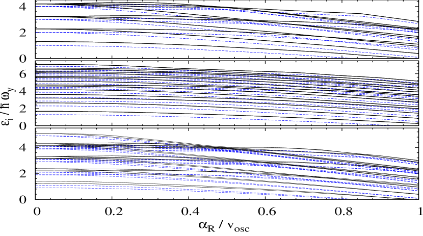
Figure 1: The self-consistent single-particle energy levels, $\varepsilon_{i}$, divided by $\hbar\omega_{y}$ are compared for interacting $g_{s}=0.5$ (black solid) and non-interacting $g_{s}=0.0$ (blue dashed) particles. The parameters are $N=20$, $\omega_{x}=\omega_{y}$, $h=0$ (upper panel), $N=30$, $\omega_{x}=1.57\omega_{y}$, $h=0$ (middle panel), and $N=22$, $\omega_{x}=\omega_{y}$, $h=0.1$ (lower panel).

Figure 2: The difference between the single-particle energy levels (divided by $\hbar\omega_{y}$) of interacting and non-interacting systems as function of the dimensionless interaction strength $g_{s}$. The number of particles is $N=20$, the harmonic trap is cylindrical ($\omega_{x}=\omega_{y}$), the Zeeman strength is $h=0$. The upper, middle and lower panels are for $\alpha_{R}=0.25,0.5,0.75$ in the units of $v_{osc}=\sqrt{\frac{2\hbar\omega_{y}}{m}}$, respectively.

In fig. 1 we compare sets of $\varepsilon_{i}$ for interacting and non-interacting particles, where the latter case was also discussed in Refs. marchukov2013 ; marchukov2014 ; marchukov2014a . The upper panel displays the simplest case of a cylindrical oscillator ($\omega_{x}=\omega_{y}$) and no Zeeman field. We choose the particle number $N=20$ since it completely fills the first $4\times 2$ degenerate shells (oscillator quantum number is 4) for $\alpha_{R}=0$. The time-reversal double degeneracy is present for all levels but the oscillator degeneracy is lifted for finite $\alpha_{R}$. The overall behavior is that the repulsion shifts all energies upwards by an amount roughly independent of spin-orbit coupling, but with a tendency of decreasing the shift as $\varepsilon_{i}$ increase. The usual avoided crossings appear with a tendency to be more pronounced for finite $g_{s}$ in the regions of high energy levels density as seen for $\alpha_{R}\simeq 0.5v_{osc}$.

In the middle panel of fig. 1 we start with an “almost irrational” frequency ratio to break as many geometrical degeneracies as possible by deforming. The particle number is also increased to $N=30$ to see more occupied levels. The overall behavior is now at first glance more complicated due to more levels. However, the shifts of the energy levels due to the repulsion are again very regular, and the very few avoided crossings also lead to smoother behavior of the energy levels as a function of $\alpha_{R}/v_{osc}$. It is less visible on fig. 1, but the energy shifts diminish with increasing single-particle energy, as consistent with less effect on unoccupied levels with increasing distance from the Fermi level.

In the lower panel of fig. 1 we break the time-reversal symmetry but stay cylindrical. The energy levels are not doubly degenerate anymore except for $\alpha_{R}=0$. However, since $J_{z}$ is still a good quantum number the energy levels from different total angular momentum multiplets are allowed to cross for finite values of $\alpha_{R}$. The particle number of $N=22$ only partially fill the last oscillator shell for $\alpha_{R}=0$. The picture appears to be more complicated but in fact only due to the doubling of the visible levels. The constant energy shifts with $\alpha_{R}$ and their decrease with $\varepsilon_{i}$ remain.

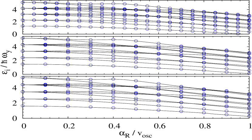
Figure 3: The single-particle energy levels (divided by $\hbar\omega_{y}$) of interacting systems as function of the dimensionless spin-orbit coupling strength $\alpha_{R}/v_{osc}$. The number of particles is $N=20$, the harmonic trap is cylindrical ($\omega_{x}=\omega_{y}$), the Zeeman strength is $h=0$. The blue circles are the first order perturbation results, and the black curves are from the Hartree-Fock solutions. The upper, middle and lower panels are for $g_{s}=0.5,0.75,1.0$, respectively.

To assess more directly the effect of the two-body repulsion we show in fig. 2 the difference between non-interacting and self-consistent Hartree-Fock single-particle energies as functions of the dimensionless interaction strength $g_{s}$. The dependence is similar for the different spin-orbit strengths with the obvious increase from zero. The curves are denser in the lowest parts of the figure where the largest single-particle energies appear, and thereby demonstrating that the effect decreases with increasing energy. In any case, we find that all these curves increase almost precisely linearly up to rather large strengths, $g_{s}$. This strongly suggests that perturbation also would be accurate in the same parameter range.

We can also compare the approximation (21) with the difference between the interacting and non-interacting single-particle levels. For instance, for $N=20$ and $g_{s}=0.5$ the estimate is $V_{pert}=0.188$ (in units of $\hbar\omega$). From the fig. 2 we see that this value is rather close to the exact value of the shift, which means that our crude approximation in the end is quite accurate.

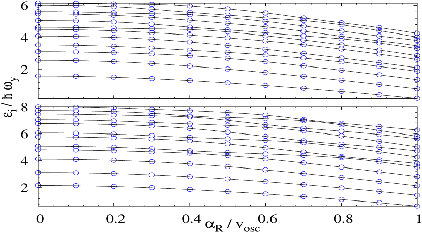
Figure 4: The single-particle energy levels (divided by $\hbar\omega_{y}$) of interacting systems as function of the dimensionless spin-orbit coupling strength $\alpha_{R}/v_{osc}$. The number of particles is $N=20$, the interaction strength is $g_{s}=0.5$ and the Zeeman strength is $h=0$. The upper and lower panel are for deformed traps with $\omega_{x}=1.57\omega_{y}$ and $\omega_{x}=2.71\omega_{y}$.

We therefore turn to compare the Hartree-Fock spectra with the lowest order perturbation results (19). The results are shown in fig. 3 for different interaction strengths, $g_{s}$. The agreement is remarkably good, and the perturbation treatment is rather accurate for all the computed values of $g_{s}\lesssim 1$. Deviations increase marginally, but hardly visible on the figure, when $g_{s}$ approaches unity, $g_{s}\to 1$. Thus, the full parameter range can be concluded to be in the weakly repulsive regime. The perturbation theory also provides a good approximation for deformed traps. This can be seen in fig. 4 for two non-integer frequency ratios, and still for time-reversal symmetric systems. The interaction strength is moderate but the agreement is very similar to the more degenerate cases in fig. 3.

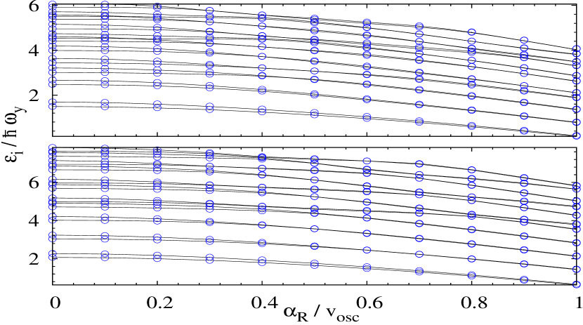
Figure 5: The single-particle energy levels (divided by $\hbar\omega_{y}$) of interacting systems as function of the dimensionless spin-orbit coupling strength $\alpha_{R}/v_{osc}$. The number of particles is $N=20$, the interaction strength is $g_{s}=0.5$ and the Zeeman strength is $h=0.1$. The upper and lower panels are for deformations $\omega_{x}=1.57\omega_{y}$ and $\omega_{x}=2.71\omega_{y}$, respectively.

Finally, we investigate the influence of the remaining one-body parameter, that is the Zeeman field, $h$, which lifts the time-reversal symmetry and the corresponding degeneracy. The interplay between deformation, spin-orbit terms and Zeeman effect is seen in the self-consistent solution shown in figs. 5 and 6. Comparing to fig. 4, we first notice that the main features are maintained, except of course the lifting of the degeneracy. The comparison between two-body interacting and non-interacting cases again show an overall upwards shift of all levels in the spectra by inclusion of the repulsion. There is also a similar tendency of a decreasing shift with increasing $\varepsilon_{i}$.

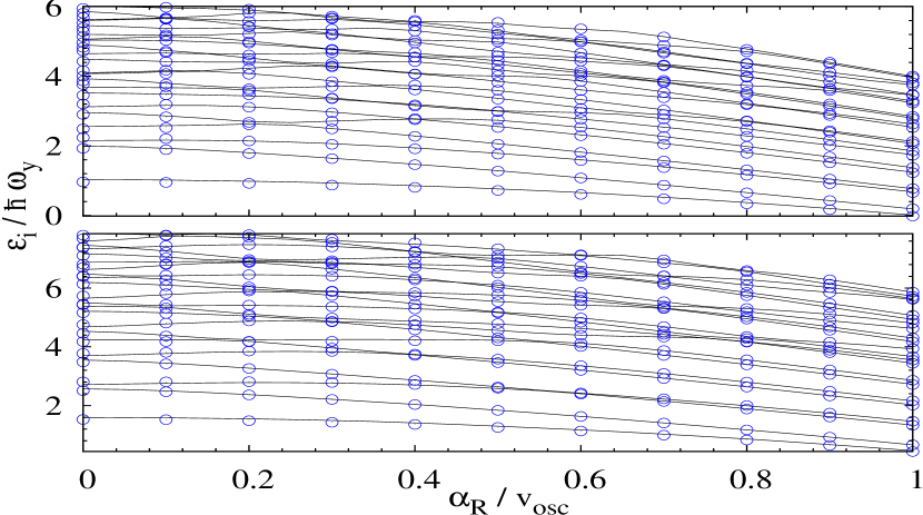
Figure 6: The single-particle energy levels (divided by $\hbar\omega_{y}$) of interacting systems as function of the dimensionless spin-orbit coupling strength $\alpha_{R}/v_{osc}$. The number of particles is $N=20$, the interaction strength is $g_{s}=0.5$ and the Zeeman strength is $h=0.6$. The upper and lower panels are for deformations $\omega_{x}=1.57\omega_{y}$ and $\omega_{x}=2.71\omega_{y}$, respectively.

Increasing the magnetic field from $h=0.1\hbar\omega_{y}$, fig. 5, to $h=0.6\hbar\omega_{y}$, fig. 6, substantially splits the previously Kramers degenerate levels. This is most clearly seen for the lowest level which is substantially below its previous time-reversed partner for small $\alpha_{R}$. We also note that this split decreases systematically for all levels with increasing $\alpha_{R}$. Finally, it is remarkable that the more complicated perturbation treatment of the two-body interaction still is fairly accurate even for relatively large $h$ and moderate to substantial $g_{s}$-values.

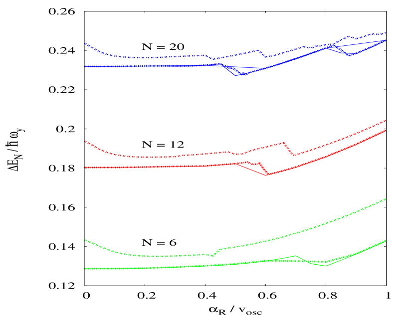
Figure 7: The total energy difference (divided by $\hbar\omega_{y}$) per particle as function of the dimensionless spin-orbit coupling strength $\alpha_{R}/v_{osc}$ from non-interacting to self-consistent Hartree-Fock solution. The system is cylindrical ($\omega_{x}=\omega_{y}$) and the repulsive strength is $g_{s}=0.5$. The number of particles are $N=6$ (green, lower manifold), $N=12$ (red, middle manifold), and $N=20$ (blue, upper manifold). The Zeeman strength is $h=0$ (full), $h=0.1\hbar\omega_{y}$ (dashed), and $h=0.6\hbar\omega_{y}$ (dotted).

The total energy of the system is a revealing quantity, but as we are interested in the effects of the two-body repulsion, we prefer to show the total energy difference between interacting and non-interacting systems per particle number

$$\Delta E_{N}=\frac{1}{N}(E_{N}-\sum_{j=1}^{N}\varepsilon^{0}_{j}),$$ (22)

where $\varepsilon^{0}_{j}$ are the single-particle eigenenergies of the non-interacting Hamiltonian and $E_{N}$ is the total energy of the interacting $N$-body system (12). In fig. 7 we present the results for a cylindrical ($\omega_{x}=\omega_{y}$) system with moderate repulsion and varying the Zeeman field. We first notice the very weak dependence on the spin-orbit strength for all cases. We also see that even when the total energy difference is divided by $N$ we see an increase with particle number which is less than another factor of $N$. Thus, the energy difference is increasing with $N$ by a power between $1$ and $2$, i.e. $\Delta E_{N}\propto N^{\delta}$, $1\leq\delta\leq 2$. The rapid decrease of the energy differences correspond to the points of spectra where many levels come close to each other. The small Zeeman strength $h=0.1\hbar\omega_{y}$ does not affect the total energy difference much, except for the points where the Fermi energy is in the vicinity of the avoided crossings. The level repulsion in a system with broken time-reversal symmetry is weaker and the additional smaller fluctuations of the total energy differences can be seen, especially for stronger Zeeman field, e.g. $h=0.6\hbar\omega_{y}$.

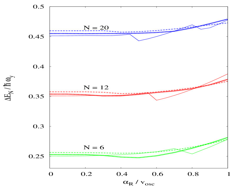
Figure 8: The total energy difference (divided by $\hbar\omega_{y}$) per particle as function of the dimensionless spin-orbit coupling strength $\alpha_{R}/v_{osc}$ from non-interacting to self-consistent Hartree-Fock solution. The Zeeman strength is $h=0$ and the interaction strength is $g_{s}=1$. The deformations are cylindrical ($\omega_{x}=\omega_{y}$) (full), $\omega_{x}=1.57\omega_{y}$ (dashed), and $\omega_{x}=2.71\omega_{y}$ (dotted).

The energy difference is obviously increasing with the strength of the repulsion as seen by the larger numerical values on the vertical axis in fig. 8. The deformation dependence is in contrast very weak for all investigated particle numbers. In both figs. 7 and  8 we see a few abrupt changes of the energy at different spin-orbit couplings depending on $N$. They arise when two single-particle levels avoid crossing each other at the Fermi energy. The last occupied single-particle wave function changes structure over a small range of coupling strengths precisely in these regions. For a relatively weak interaction this happens very quickly over a very small change of spin-orbit parameter. Therefore the abrupt change would disappear only with a very much finer grid, and this continuity would only be invisible on a much smaller scale than exhibited on these figures. Other avoided crossings below the Fermi energy do not change the total antisymmetrized product wave function in this abrupt manner because the system populates those levels both before and after the crossings. The same conclusion of no abrupt changes is even more obvious for crossings above the Fermi level since none of them can influence the total wave function.

III.3 Statistical analysis

In this subsection we provide results of the statistical analysis of the calculated spectra for the interacting system. The spacing distribution, $P(S)$, of the nearest neighbor energy spacing, $S$, can provide valuable insight into the dynamical properties of the system haake2001 . The distribution and the nearest neighbor measure are defined as dimensionless and scale-independent values through a rather involved standard procedure in these statistical analyses. The distribution is then normalized and the average level spacing is equal to unity. The procedure is in literature referred to as “unfolding”.

The Poisson distribution, $P(S)=e^{-S}$, corresponds to the classically regular behavior and the class of Wigner distributions, $P(S)\sim S^{\beta}e^{-S^{2}}$, serve as a so-called quantum signature of chaos haake2001 ; berry1987 . Here the values $\beta=1,2,4$ corresponds to different symmetries of the system  haake2001 . Such a statistical analysis was performed in Ref. marchukov2014a for non-interacting particles in a deformed harmonic trap where each particle is subject to a one-body spin-orbit interaction. It was shown that the nearest neighbor energy spacing reproduces the $\beta=4$ Wigner distribution,

$$P(S)=\frac{2^{18}S^{4}}{3^{6}\pi^{3}}\mathrm{exp}\left(-\frac{64S^{2}}{9\pi}\right),$$ (23)

for specific values of the potential parameters. Here we investigate how the two-body interaction affects these energy level distributions.

The statistical analysis employs a non-trivial procedure to extract the significant scale independent distributions  haake2001 . The basic ingredients are the single-particle energies in an appropriate energy interval. It is required for the analysis that the average energy spacing is normalized to unity. This procedure is usually called unfolding of the spectrumhaake2001 . The resulting spectrum is dimensionless and so is the nearest neighbor spacing $S$. The choice of the energy interval is restricted to the levels that are sufficiently accurately determined. This implies that the highest single-particle energies $\varepsilon_{i}$ should be avoided since they reflect properties of the basis more than effects of the interaction. We have therefore always chosen the upper boundary of the energy window as less than half of the number of basis states.

The mean-field solutions for finite two-body interaction depend on particle number. The dynamic behavior reflected in the nearest neighbor energy distribution must be extracted by use of an energy interval corresponding to the allowed excitation energies of the entire system. A reasonable choice is therefore to have roughly the same number of levels above as below the Fermi energy. This requires that the number of particles is large enough to allow us a reasonably accurate and well defined statistical analysis.

The self-consistent calculations for deformed potentials are time consuming and quickly increasing with particle number. The systematic investigation in the previous subsections of spectra and energies as functions of the many interaction parameters were therefore carried out and reported for a relatively small number of particles. For the statistical analyses in the present subsection we have chosen to use particle number $N=100$ for selected interaction parameters. We used more than 575 basis states for the diagonalization with a maximum energy corresponding to level number $200$, that is as many above as below the Fermi level. The accuracies of the spectra are discussed in section IIIA.

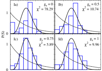
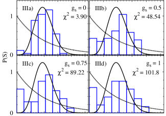
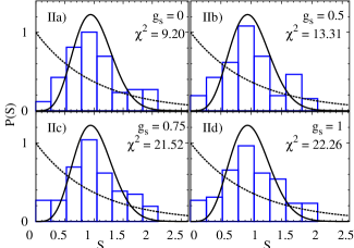
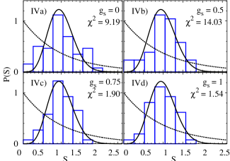
Figure 9: The nearest neighbor level spacing distribution $P(S)$ for different sets of parameter values. Roman numerals correspond to different cases of deformation and spin-orbit coupling strength: I) $\omega_{x}/\omega_{y}=1.57$, $\alpha_{R}/v_{osc}=0.3$, II) $\omega_{x}/\omega_{y}=1.57$, $\alpha_{R}/v_{osc}=0.5$, III) $\omega_{x}/\omega_{y}=2.71$, $\alpha_{R}/v_{osc}=0.21$, and IV) $\omega_{x}/\omega_{y}=2.71$, $\alpha_{R}/v_{osc}=0.5$. The letters a-d correspond to different two-body interaction strength: a) $g_{s}=0$, b) $g_{s}=0.5$, c) $g_{s}=0.75$, and d) $g_{s}=1$. The external magnetic field is $h=0$. The distributions are compared to the Poisson (dashed line) and $\beta=4$ Wigner of eq. (23) (solid line) distributions. We used 100 non-degenerate energy levels in the analysis.

In fig. 9 we show the distributions for two trap deformations, $\omega_{x}/\omega_{y}=1.57$ (I-II) with spin-orbit strengths $\alpha_{R}/v_{osc}=0.3,0.5$, respectively, and $\omega_{x}/\omega_{y}=2.71$ (III-IV), with $\alpha_{R}/v_{osc}=0.21,0.5$, respectively. For each set we varied the two-body interaction strengths $g_{s}$. The deformations are chosen to be relatively small numbers but far away from integer frequency ratios. The values of the spin-orbit coupling strength are chosen such that we observe distributions different from and similar to the Wigner distribution in eq. (23).

In fig. 9I) we see that for the given deformation, $\omega_{x}/\omega_{y}=1.57$, and spin-orbit coupling strength, $\alpha_{R}=0.3~{}v_{osc}$, the distribution for $g_{s}=0$ is far from eq. (23). However, as the repulsion increases towards $g_{s}=0.75$, we notice that the Wigner distribution is approached but for larger $g_{s}=1$ this similarity seems to disappear again. For the same deformation in fig. 9II), but for larger spin-orbit strength, $\alpha_{R}=0.5~{}v_{osc}$, the histogram is relatively close to a Wigner distributions for $g_{s}=0$, and in fact more or less conserve the character of this distribution as $g_{s}$ increases. In fig. 9III) the approximate Wigner distribution at $g_{s}=0$ is quickly destroyed as $g_{s}$ increases. In fig. 9IV) we notice the opposite effect that the Wigner distribution is much better reproduced for $g_{s}=0.75$ and $g_{s}=1.0$ than for $g_{s}=0$.

These intuitive and visual qualitative evaluations of the distributions can be made quantitative by chi-squared analyses. The measure of similarity between histograms and Wigner distributions can be defined as in reichl1992 , that is

$$\chi^{2}=\sum_{i=1}^{i_{max}}\frac{(p_{i}-\nu_{i})^{2}}{\nu_{i}}\;,$$ (24)

where $i_{max}$ is a number of bins, $p_{i}$ is the number of the data points from the histogram in the $i$th bin, and $\nu_{i}$ is the number of the data points predicted by the Wigner distribution eq. (23).

The results are shown on each of the inserted figures in the main fig. 9. Fortunately, the sizes of the $\chi^{2}$-values correlate perfectly with our qualitative visual observations. When the Wigner distribution is most precisely reproduced the $\chi^{2}$-value is slightly below $2$, see IVc and IVd. In contrast, large deviations from the Wigner distribution easily reach values much higher than $10$ and sometimes significantly above $100$, see IIIc and IIId.

To reach the lowest values of about $2$ is not easily achieved with the measure in eq. (24), since for example a small bump at small or large $s$-values would add a rather large contribution to $\chi^{2}$. Thus, in general small deviations from the Wigner form would show up in the $\chi^{2}$-value, which therefore is a sensitive measure of an underlying chaotic dynamic behavior.

Our findings are qualitatively consistent with the results obtained in Ref. armstrong2012 for a many-fermion system in a cylindrical ($\omega_{x}=\omega_{y}$) 2D harmonic trap with an attractive short-range pairing interaction. The authors of this paper have found that the interplay between the trap and the pairing interaction is responsible for the dynamical behavior of the system. Particularly, in the case when the contributions are of comparable significance the competition produces the irregular behavior seen in the Brody distribution, which is known to be an “intermediate” one between the Poisson and Wigner distributions brody1981 ; santos2010 . Similarly, in our system the dynamical behavior is defined by the interplay between the harmonic trap, spin-orbit coupling and the two-body interaction.

IV Conclusions

The two-dimensional properties of spin-orbit coupled systems of identical fermions can be investigated experimentally. It is possible to control and independently tune several of the external one-body parameters like deformation of an oscillator trap, the magnetic field for Zeeman splitting, form and strength of the spin-orbit coupling, and on top also the interaction between pairs of particles. The two-body interaction introduces a particle number dependence of structure and properties. The first attempt to understand the interplay between all these terms of the Hamiltonian is to compute the average structure by use of mean-field theory.

We write down the self-consistent Hartree-Fock equations with one-body terms in the Hamiltonian. The formulation necessarily involves a two-component wave function formally corresponding to spin-up or spin-down. We discuss symmetries related to each of the one- and two-body potentials, and relate to the properties for the Hartree-Fock equations.

The single-particle energy spectra exhibit the same features as the non-interacting systems, that is with level crossings and low and high level-density regions corresponding to more or less stability against changes due to other interactions or other degrees of freedom. The overall change from the two-body repulsive potential is a shift upwards of all spectra. The details of these shifts are very well accounted for by perturbation up to moderate sizes of the two-body interaction.

The many details of the spectra can be collected in the total energy which is a more macroscopic quantity. Furthermore, we eliminate most of the overall spectral shift-dependence by comparing the energy difference due to the repulsion as function of the various parameters. The energy difference increases rather strongly with the repulsive strength, that is very crudely as the square of the strength. The numerical results for the energy difference most often only varies by less than about 15% as function of deformation and spin-orbit coupling strength in most cases. In contrast, increasing the Zeeman strength strongly suppresses the energy difference which implies that the levels actively involved in the two-body coupling move apart, and the repulsion is effectively reduced.

The dynamic behavior of the interacting system is analyzed statistically through nearest neighbor energy level distributions of the mean-field single-particle energies. These distributions are for moderate repulsion somewhat similar to the non-interacting system. The Wigner distribution associated with irregular behavior turned out to occur for special parameters. When the two-body repulsion is turned on these Wigner distributions may disappear. However, occasionally Wigner distributions appear for intermediate strength repulsion, while absent for both smaller and larger repulsion.

In conclusion, we have shown that the repulsive short-range two-body interaction can be treated perturbatively for small and moderate strengths. The spectra are first of all shifted depending somewhat on interaction parameters. Statistically irregular behavior may turn into regular behavior, and vice versa, as function of the repulsive strength. Our results provide evidence of possible quantum chaotic behaviour in these spin-orbit coupled and deformed systems also in the presence of repulsive two-body interactions of small to intermediate strength. Cold atoms with spin-orbit coupling could thus provide a very flexible venue for studying quantum chaos.

References

- (1) W. Ketterle and M. W. Zwierlein, Nuovo Cimento Rivista Serie 31, 247 (2008).
- (2) I. Bloch, J. Dalibard and W. Zwerger, Rev. Mod. Phys. 80, 885 (2008).
- (3) T. Esslinger, Ann. Rev. Cond. Mat. Phys. 1, 129 (2010).
- (4) J. I. Cirac and P. Zoller, Nature Phys. 8, 264 (2012).
- (5) Y.-J. Lin et al, Phys. Rev. Lett. 102, 130401 (2009).
- (6) Y.-J. Lin, R. L .Compton, K. Jiménez-García, J. V. Porto and I. B. Spielman, Nature 462, 628 (2009).
- (7) Y.-J. Lin, K. Jiménez-García and I. B. Spielman, Nature 471, 83 (2011).
- (8) M. Aidelsurger, Phys. Rev. Lett. 107, 255301 (2011).
- (9) J.-Y. Zhang et al, Phys. Rev. Lett. 109, 115301 (2012).
- (10) P. Wang et al., Phys. Rev. Lett. 109, 095301 (2012).
- (11) L. Cheuk et al., Phys. Rev. Lett. 109, 095302 (2012).
- (12) H. Hu and S. Chen, arXiv:1302.5933 (2013).
- (13) J. Larson and E. Sjöqvist, Phys. Rev. A 79, 043627 (2009).
- (14) X. Y. Yin, S. Gopalakrishnan and D. Blume, Phys. Rev. A 89, 033606 (2014).
- (15) O. V. Marchukov, A. G. Volosniev, D. V. Fedorov, A. S. Jensen and N. T. Zinner, J. Phys. B: At. Mol. Opt. Phys. 46, 134012 (2013).
- (16) S. M. Reimann and M. Manninen, Rev. Mod. Phys. 74, 1283 (2002).
- (17) S. Avetisyan, P. Pietiläinen, and T. Chakraborty, Phys. Rev. B 85, 153301 (2012).
- (18) E. I. Rashba, Sov. Phys. Solid State 2, 1109 (1960).
- (19) G. Dresselhaus, Phys. Rev. 100, 580 (1955).
- (20) O. V. Marchukov, A. G. Volosniev, D. V. Fedorov, A. S. Jensen and N. T. Zinner, J. Phys. B: At. Mol. Opt. Phys. 47, 195303 (2014).
- (21) R. S. Markiewicz, Phys. Rev. E 64, 026216 (2001).
- (22) H. Yamasaki, Y. Natsume, A. Terai and K. Nakamura, Phys. Rev. E 68, 046201 (2003).
- (23) E. Majerníková and S. Shrypko, Phys. Rev. E 73, 057202 (2006).
- (24) E. Majerníková and S. Shrypko, Phys. Rev. E 73, 066215 (2006).
- (25) Q. Guan, X. Y. Yin, S. E. Gharashi and D. Blume, J. Phys. B 47, 161001 (2014).
- (26) X. Cui and W. Yi, Phys. Rev. X 4, 031026 (2014).
- (27) P. J. Siemens and A. S. Jensen: Elements of Nuclei: Many-Body Physics with the Strong Interaction, (Redwood City, Calif, Addison-Wesley Pub. Co., 1987).
- (28) M. Olshanii and L. Pricoupenko, Phys. Rev. Lett. 88, 010402 (2002).
- (29) M. Valiente, Phys. Rev. A 85, 014701 (2012).
- (30) D. S. Petrov, M. Holzmann, and G. V. Shlyapnikov, Phys. Rev. Lett. 84, 2551 (2000).
- (31) D. S. Petrov and G. V. Shlyapnikov, Phys. Rev. A 64, 012706 (2001).
- (32) M. Valiente, N. T. Zinner, and K. Mølmer, Phys. Rev. A 86, 043616 (2012).
- (33) H. Hu, B. Ramachandhran, H. Pu and X.-J. Liu, Phys. Rev. Lett. 108, 010402 (2012).
- (34) L. D. Landau and E. M. Lifshitz: Quantum Mechanics (Non-relativistic Theory), (Pergamon, Oxford, 1977).
- (35) J. J. Sakurai: Modern Quantum Mechanics, (Addison-Wesley Publishing Company, Reading, USA, Revised edition 1994).
- (36) M. Abramowitz and I. A. Stegun: Handbook of Mathematical Functions with Formulas, Graphs, and Mathematical Tables, (Dover Publications, New York, 10th Ed., 1972).
- (37) O. V. Marchukov, A. G. Volosniev, D. V. Fedorov, A. S. Jensen and N. T. Zinner, Few-Body Syst. 55, 1045 (2014).
- (38) F. Haake: Quantum Signatures of Chaos, (Springer-Verlag Berlin Heidelberg, 2nd edition 2001).
- (39) M. V. Berry, Proc. R. Soc. Lond. A 413, 183 (1987).
- (40) Reichl L. E.: The Transition to Chaos: Conservative Classical Systems and Quantum Manifestation (Springer-Verlag, 2nd edition 2004).
- (41) J. R. Armstrong, S. Åberg, S. M. Reimann and V. G. Zelevinsky, Phys. Rev. E 86, 066204 (2012).
- (42) T. A. Brody, J. Flores, J. B. French, P. A. Mello, A. Pandey and S. S. M. Wong, Rev. Mod. Phys. 53, 3 (1981).
- (43) L. F. Santos and M. Rigol, Phys. Rev. E 81, 036206 (2010).