Bifurcation of Nonlinear Bloch Waves from the Spectrum in the Gross-Pitaevskii Equation

Abstract.

We rigorously analyze the bifurcation of stationary so called nonlinear Bloch waves (NLBs) from the spectrum in the Gross-Pitaevskii (GP) equation with a periodic potential, in arbitrary space dimensions. These are solutions which can be expressed as finite sums of quasi-periodic functions, and which in a formal asymptotic expansion are obtained from solutions of the so called algebraic coupled mode equations. Here we justify this expansion by proving the existence of NLBs and estimating the error of the formal asymptotics. The analysis is illustrated by numerical bifurcation diagrams, mostly in 2D. In addition, we illustrate some relations of NLBs to other classes of solutions of the GP equation, in particular to so called out–of–gap solitons and truncated NLBs, and present some numerical experiments concerning the stability of these solutions.

1. Introduction

The nonlinear Schrödinger/Gross–Pitaevskii (GP) equation in $d\in\mathbb{N}$ dimensions,

(1.1) $${\rm i}\partial_{t}\psi=\Delta\psi-V(x)\psi-\sigma|\psi|^{2}\psi,\quad x\in\mathbb{R}^{d},\ t\in\mathbb{R},$$

with a real potential $V:\mathbb{R}^{d}\to\mathbb{R}$ is a canonical model in mathematics and physics. It appears in various contexts, e.g., nonlinear optics [33, 17], and Bose–Einstein condensation [26, 4]. See also, e.g., [34, 40, 19] for mathematical and modeling background. Plugging ${\rm e}^{{\rm i}\omega t}\varphi(x)$ into (1.1), where $\omega/(2\pi)$ is the frequency of time–harmonic waves in nonlinear optics, and where $\omega$ is called the chemical potential in Bose–Einstein condensation, we obtain the stationary problem

(1.2) $$\omega\varphi+\Delta\varphi-V(x)\varphi-\sigma|\varphi|^{2}\varphi=0.$$

Here we consider the case that the potential $V$ is real and periodic. For simplicity, we let $V$ be $2\pi-$periodic in each coordinate direction, i.e.,

$$V(x+2\pi e_{j})=V(x)\quad\text{ for all }x\in\mathbb{R}^{d},j\in\{1,\dots,d\},$$

where $e_{j}$ denotes the $j$-th Euclidean unit vector in $\mathbb{R}^{d}$. In other words, we consider the periodic lattice $2\pi\mathbb{Z}^{d}$. We make the basic assumption that $V\in H^{s-2}({\mathbb{P}})$ for some $s>\frac{d}{2}$, where ${\mathbb{P}}=(-\pi,\pi]^{d}$. This smoothness assumption on $V$ ensures $H^{s}({\mathbb{P}})$-smoothness of linear Bloch waves, i.e., solutions of (1.2) with $\sigma=0$. See §1.1 for a review of spectral properties of

$$L=-\Delta+V$$

and linear Bloch waves. For suitable $V$ the spectrum of $L$ shows so called spectral gaps and in recent years a focus has been on the bifurcation of so called gap solitons from the the zero solution at band edges into the gaps. These are localized solutions, which, in the near edge asymptotics have small amplitude and long wave modulated shape. In detail, the asymptotic expansion at $\omega=\omega_{*}+\varepsilon^{2}\Omega$ with $\Omega=\pm 1$ is

(1.3) $$\varphi(x)\sim\varepsilon\sum_{j=1}^{N}A_{j}(\varepsilon x)\xi_{n_{j}}(k^{(j)};x),$$

where $\xi_{n_{j}}(k^{(j)};\cdot)$, $j=1,\ldots,N$ are Bloch waves at the edge $\omega_{*}$, and the $A_{j}$ are localized solutions of a system of (spatially homogeneous) nonlinear Schrödinger equations. See, for instance, [32, 12, 15, 23], and the references therein.

Here we seek solutions of (1.2) which can be expressed as finite a sum of $M$ quasi-periodic functions and call such solutions nonlinear Bloch waves (NLBs), with quasi–periodicities determined from a selected finite subset of the Bloch waves at $\omega$. NLBs have been studied in, for instance, [12, 38, 42, 43, 9], where in [38, 42, 43] the approaches are numerical and formal. They have been observed even experimentally, see e.g. [10] for experiments in Bose-Einstein condensates. In [12] the special case of a bifurcation of NLBs into an asymptotically small spectral gap for a separable periodic potential in two dimensions is studied rigorously. In [9] the bifurcation of single component ($M=1$) NLBs in one dimension is proved, including results on secondary bifurcations and exchange of stability. Similarly to Bloch waves in linear lattices NLBs can be understood as the fundamental bounded oscillatory states of the nonlinear system. From the applied point of view one motivation for studying NLBs is the continuation of gap–solitons to “out-of-gap” solitons, i.e., the continuation of localized solutions from one band edge across the gap and into the spectrum on the other side of the gap, where their tails start interacting with the NLBs. For this reason, the study of bifurcation of NLBs from the zero–solution has been mostly restricted to band edges. Here we show that nonlinear Bloch waves bifurcate in $\omega$ from generic points in the spectrum of $L$, and give their asymptotic expansions in terms of solutions of the so called algebraic coupled mode equations (ACME), together with error estimates.

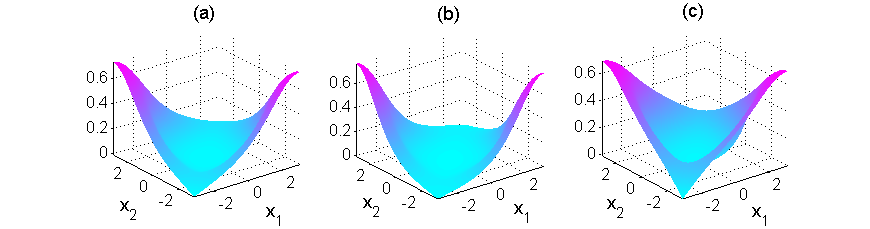
In addition to the rigorous analysis we illustrate our results numerically. For this we focus on 2D, as this is much richer than 1D, and use the same potential as in [15], i.e.

(1.4) $$V(x)=1+4.35W(x_{1})W(x_{2}),\quad x\in[-\pi,\pi]^{2}$$

with

$$W(s)=\frac{1}{2}\left[\tanh\left(7\left(s+\frac{3\pi}{5}\right)\right)+\tanh\left(7\left(\frac{3\pi}{5}-s\right)\right)\right].$$

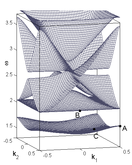
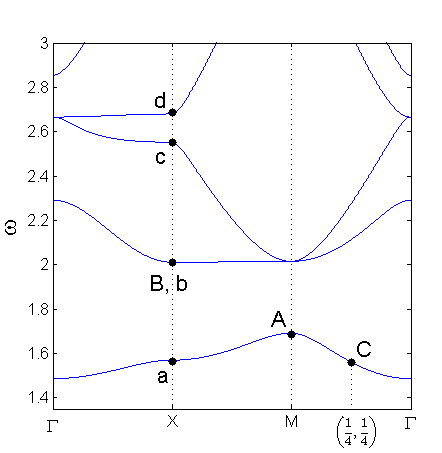
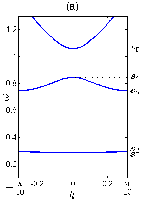
This represents a square geometry with smoothed-out edges. The function in (1.4) is extended periodically to $\mathbb{R}^{2}$ to obtain $V:\mathbb{R}^{2}\to\mathbb{R}$. The numerical band structure of $L$ over the Brillouin zone $\mathbb{B}:=(-1/2,1/2]^{d}$, and also along the boundary of the irreducible Brillouin zone, is plotted in Fig. 1(a),(b), respectively. We denote the so called high symmetry points in $\mathbb{B}$ for $d=2$ by

$$\Gamma:=(0,0),X:=(1/2,0),X^{\prime}:=(0,1/2),\quad\text{and }M:=(1/2,1/2).$$

(a)	(b)

Figure 1. (a): Band structure of $L$ over the Brillouin zone $\mathbb{B}$ for the periodic potential (1.4); (b): along the boundary $\Gamma-X-M-\Gamma$ of the, so called, irreducible Brillouin zone.

Example 1.

Figure 2 shows a numerical bifurcation diagram of single component ($M=1$) NLBs for $k=X$, calculated with the package pde2path [36, 13], together with example plots on the bifurcating branches. A branch of NLBs bifurcates from the zero solution at $\omega=\omega_{*}$ for any $\omega_{*}$ attained by one of the band functions at $k=X$, i.e. at the $\omega-$coordinate of any of the points $a,b,c,d$ in Fig. 1 (b). See §1.1 for the definition of band functions.

Figure 2. Example 1: Bifurcation diagram of the first four bifurcating branches for $k=X$, i.e. branches bifurcating from points a-d in Fig. 1 (b). Spectral bands are indicated by the black dashed line. The sign $\pm$ in the branch labels stands for $\sigma=\pm 1$. Small panels: example solution plots of NLBs from the bifurcation diagram, over the fundamental cell $x\in(-\pi,\pi)^{2}$. At bifurcation we choose a real Bloch wave. Then the imaginary parts are small near bifurcation, and we only plot them for a$\pm$. Roughly horizontal axis corresponds to $x_{1}$ in all plots.

In §7 we explain the method behind Fig. 2, and study in detail the bifurcations of NLBs at the points marked A,B,C in Fig. 1(b), relating the numerical calculations to our analysis.

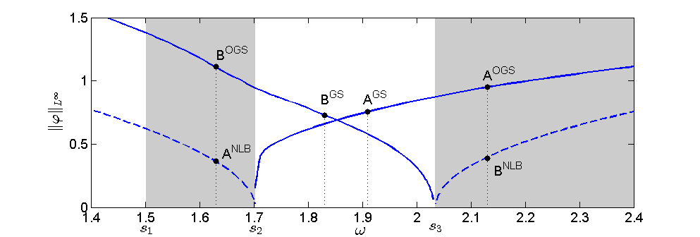
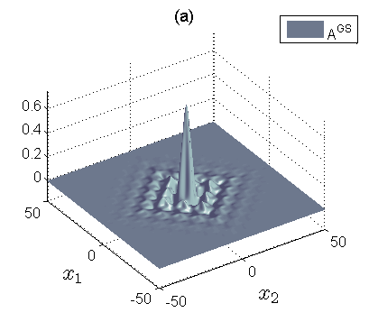
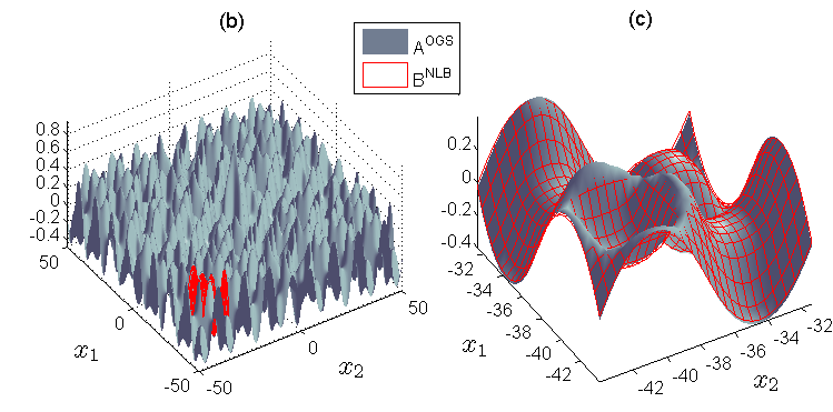
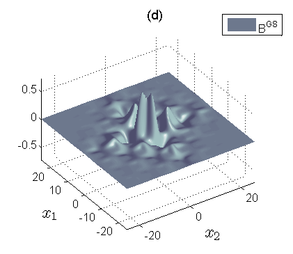
As already said, one motivation for studying NLBs are the intriguing properties of their interaction with localized solutions, which we illustrate numerically in §8. For instance, when a gap soliton is continued from the gap into the spectrum, we get a so called “out–of–gap” soliton (OGS) with oscillating (delocalized) tails, see also [41, 24]. In 1D, numerically these OGS can be seen to be homoclinic orbits approaching NLBs, and essentially the same happens in 2D. Moreover, the NLB can form building blocks of so called truncated NLBs (tNLBs), see also [4, 38]. These are localized solutions for $\omega$ in a gap which are close to a NLB on some finite interval but approach $0$ as $|x|\to\infty$. Then, continuing a branch of tNLBs from the gap into the spectrum, the same interaction scenario as for GS happens, i.e., the tails of the tNLBs pick up NLBs bifurcating from the gap edge into the spectrum, and the tNLBs become delocalized, for which we use the acronym dtNLB. Note that both gap solitons and tNLBs have been observed experimentally, see e.g. [5] for experiments in optical lattices. However, even in 1D at present it is unclear how to analyze OGS, tNLBs and dtNLBs rigorously, i.e., so far there only exist heuristic asymptotics, see §8 for further comments.

Stability of most of these solutions is an open problem. Thus, at the end of the paper we also give a numerical outlook on this, and obtain stability of some NLBs in 1D, and, consequently, stability of some tNLBs and some OGS and dtNLBs. In 2D, we did not find stable NLBs for the potential $V$ from (1.4), and we close with summarizing the open questions. The broad spectrum of applications of NLBs clearly motivates our rigorous bifurcation analysis.

In the remainder of this introduction we explain the linear band structure, a simple analytical bifurcation result, formulate the main theorem, and describe the structure of the paper in more detail.

1.1. Linear Bloch waves

For $k$ in the Brillouin zone, $k\in\mathbb{B}:=(-1/2,1/2]^{d}$, consider the Bloch eigenvalue problem

(1.5) $$(-\Delta+V(x))\xi_{n}(x,k) =\omega_{n}(k)\xi_{n}(x,k),\quad x\in{\mathbb{P}}$$

$$\xi_{n}(x+2\pi e_{m},k) =e^{2\pi{\rm i}k_{m}}\xi_{n}(x,k),\quad m\in\{1,\dots,d\},$$

where $e_{m}$ is the $m-$th Euclidean unit vector in $\mathbb{R}^{d}$. The spectrum of $L=-\Delta+V$ is continuous and is given by the union of the bands defined by the band structure $(\omega_{n}(k))_{n\in\mathbb{N}}$, i.e.

$$\sigma(L)=\bigcup_{\begin{subarray}{c}n\in\mathbb{N}\\ k\in\mathbb{B}\end{subarray}}\omega_{n}(k)=\bigcup_{l\in\mathbb{N}}[s_{2l-1},s_{2l}],\ \text{ where }s_{2l-1}<s_{2l}\leq s_{2l+1}\ \text{ for all }l\in\mathbb{N},$$

see Theorem 6.5.1 in [16]. The functions $k\mapsto\omega_{n}(k)$ are called band functions. The Bloch waves $\xi_{n}(x,k)$ have the form $\xi_{n}(x,k)=p_{n}(x,k)e^{{\rm i}k\cdot x}$ with $p_{n}(x+2\pi e_{m},k)=p_{n}(x,k)$ for all $m\in\{1,\dots,d\}$ and all $x\in\mathbb{R}^{d}$. Clearly, both $\omega_{n}(k)$ and $\xi_{n}(x,k)$ are $1-$periodic in each component of $k$. We assume the normalization

$$\|\xi_{n}(\cdot,k)\|_{L^{2}({\mathbb{P}})}=\|p_{n}(\cdot,k)\|_{L^{2}({\mathbb{P}})}=1\quad\forall n\in\mathbb{N}\ \forall k\in\mathbb{B}.$$

For a given point $(k,\omega)\in\mathbb{B}\times\mathbb{R}$ in the band structure, i.e. with $\omega=\omega_{n}(k)$ for some $n\in\mathbb{N}$, also the point $(-k,\omega)$ lies in the band structure, which follows from the symmetry

(1.6) $$\omega_{n}(k)=\omega_{n}(-k)\ \text{for all}\ n\in\mathbb{N},k\in\mathbb{B}.$$

This symmetry is due to the equivalence of complex conjugation and replacing $k\mapsto-k$ in the eigenvalue problem (1.5). Hence, we also have the conjugation symmetry of the Bloch waves, namely

(1.7) $$\xi_{n}(x,k)=\overline{\xi_{n}(x,-k)}.$$

For $k\in\partial\mathbb{B}\cap\mathbb{B}$ we have $-k\in\partial\mathbb{B}\setminus\mathbb{B}$ and the point $-k$ must be understood as the $\mathbb{Z}^{d}$-periodic image within $\mathbb{B}$. When $k$ is one of the so called high symmetry points, i.e. $k_{m}\in\{0,1/2\}$ for all $m\in\{1,\dots,d\}$, then $k$ and $-k$ are identified via this periodicity. Equation (1.7) then implies that $\xi_{n}(x,k)$ is real. This can be seen directly from the eigenvalue problem (1.5), where $k_{m}\in\{0,1/2\}$ for all $m\in\{1,\dots,d\}$ implies that the boundary condition is real such that a real eigenfunction must exist. Note that the above $k-$symmetries rely only on the realness of $V$.

1.2. The Bifurcation Problem

Remark 1.

In the simplest scenario we can look for real solutions of (1.2) with the quasi-periodic boundary conditions given by a single vector $k_{*}\in\mathbb{B}$, i.e.

(1.8) $$\varphi(x+2\pi e_{m})=\varphi(x)e^{2\pi{\rm i}k_{*,m}}\quad\text{for all }x\in\mathbb{R}^{d},m\in\{1,\dots,d\}.$$

In this case the realness condition on $\varphi$ requires

(1.9) $$k_{*}\in\left\{0,\tfrac{1}{2}\right\}^{d},$$

such that the sought solution is $2\pi$-periodic or $2\pi$-antiperiodic in each coordinate direction. We study bifurcations in the parameter $\omega$. Classical theory for bifurcations at simple eigenvalues, e.g., Theorem 3.2.2 in [29], shows that if $\omega_{*}=\omega_{n_{*}}(k_{*})$ for exactly one $n_{*}\in\mathbb{N}$, i.e. $\omega_{*}$ is a simple eigenvalue of $L$ under the boundary conditions (1.8), then $\omega=\omega_{*}$ is a bifurcation point. To this end define $f(\varphi,\omega)=\omega\varphi+\Delta\varphi-V(x)\varphi-\sigma\varphi^{3}$ and study $f(\varphi,\omega)=0$ on ${\mathbb{P}}$ under the boundary conditions (1.8). We have $f(0,\omega)=0$ for all $\omega\in\mathbb{R}$ and $f_{\varphi}(0,\omega)=\omega-L$. As $\omega_{*}$ is a simple eigenvalue, we have the one dimensional kernel

$$\mbox{Ker}(f_{\varphi}(0,\omega_{*}))=\xi_{n_{*}}(x,k_{*})\mathbb{R}.$$

Because $L$ with (1.8) and (1.9) is self adjoint, we have $\mbox{ Ran}(f_{\varphi}(0,\omega_{*}))\perp_{L^{2}({\mathbb{P}})}\text{Ker}(f_{\varphi}(0,\omega_{*}))$. The transversality condition $f_{\omega\varphi}(0,\omega_{*})\xi_{n_{*}}(x,k_{*})\notin\text{Ran}(f_{\varphi}(0,\omega_{*}))$ of Theorem 3.2.2 in [29] thus holds because $f_{\omega\varphi}(0,\omega_{*})\xi_{n_{*}}(x,k_{*})=\xi_{n_{*}}(x,k_{*})\perp_{L^{2}({\mathbb{P}})}\text{Ran}(f_{\varphi}(0,\omega_{*}))$. As a result, the theorem guarantees the existence of a unique non-trivial branch of solutions bifurcating from $\omega=\omega_{*}$.

Remark 2.

Without the restriction to real solutions the eigenvalue $\omega_{*}$ is never simple due to invariances. In the real variables $\Phi:=(\varphi_{R},\varphi_{I})^{T}$, where $\varphi=\varphi_{R}+{\rm i}\varphi_{I}$, the problem becomes

$${\mathcal{G}}(\Phi,\omega)=\begin{pmatrix}\omega\varphi_{R}+\Delta\varphi_{R}-V(x)\varphi_{R}-\sigma(\varphi_{R}^{2}+\varphi_{I}^{2})\varphi_{R}\\ \omega\varphi_{I}+\Delta\varphi_{I}-V(x)\varphi_{I}-\sigma(\varphi_{R}^{2}+\varphi_{I}^{2})\varphi_{I}\end{pmatrix}=0.$$

Since (1.2) possesses the phase invariance and the complex conjugation invariance, we get that ${\mathcal{G}}$ is $O(2)$ invariant, i.e.

$${\mathcal{G}}(\gamma\Phi,\omega)=\gamma{\mathcal{G}}(\Phi,\omega)\text{ for all }\gamma\in\Gamma:=\left\{\left(\begin{smallmatrix}1&0\\ 0&-1\end{smallmatrix}\right),\left(\begin{smallmatrix}\cos\theta&-\sin\theta\\ \sin\theta&\cos\theta\end{smallmatrix}\right):\theta\in[0,2\pi)\right\}.$$

Bifurcations can now be studied using the equivariant branching lemma, see e.g. [28, §5], by restricting to a fixed point subspace of a subgroup of $\Gamma$. The only nontrivial subgroup is $\{\left(\begin{smallmatrix}1&0\\ 0&1\end{smallmatrix}\right),\left(\begin{smallmatrix}1&0\\ 0&-1\end{smallmatrix}\right)\}$ with the fixed point subspace being the vectors $\Phi$ with $\varphi_{I}=0$ corresponding to real solutions of (1.2). Therefore, this leads again to real solutions. Nevertheless, more complicated solutions than the single component ones in Remark 1 can be studied. The most general real ansatz is

(1.10) $$\varphi(x)=\sum_{j=1}^{2q+r}\varphi_{j}(x),\quad\varphi_{j}(x+2\pi e_{m})=e^{{\rm i}2\pi k_{m}^{(j)}}\varphi_{j}(x),m=1,\dots,d$$

with $q,r\in\mathbb{N}_{0}$, with $k^{(j)}\in\mathbb{B}$ for all $j=1,\dots,2q+r$, such that $k^{(j+q)}\dot{=}-k^{(j)},\varphi_{j+q}=\overline{\varphi_{j}}$ for all $j=1,\dots,q$, and with $k^{(j)}\in\{0,1/2\}^{d},\varphi_{j}(x)\in\mathbb{R}$ for $j=2q+1,\dots,2q+r$. Here $\dot{=}$ means equality modulo 1 in each coordinate. While the use of the equivariant branching lemma should describe the bifurcation problem and produce the effective Lyapunov-Schmidt reduction, we choose to carry out a detailed analysis without this tool in order to obtain more explicit results. This will allow us to provide estimates of the asymptotic approximation error.

Our aim is to prove a general bifurcation theorem for NLBs, and, moreover, to derive and justify an effective asymptotic model related to the Lyapunov-Schmidt reduction of the bifurcation problem including an estimate on the asymptotic error. In our approach we select a frequency $\omega_{*}$ in the spectrum and choose $N$ points $\{k_{*}^{(1)},\dots,k_{*}^{(N)}\}\subset\mathbb{B}$ in the level set of the band structure at $\omega_{*}$, such that for each $j$ we have $\omega_{*}=\omega_{n_{j}}(k_{*}^{(j)})$ for some $n_{j}\in\mathbb{N}$. Our method requires that each of the points $\{k_{*}^{(1)},\dots,k_{*}^{(N)}\}$ is either one of the high symmetry points $k\in\{0,1/2\}^{d}$ or belongs to a pair $k,l$ with $l\dot{=}-k$. See (H1)–(H6) on page 3.2 for a summary of our assumptions. We seek NLBs bifurcating from $\omega_{*}$ and having the asymptotic form

(1.11) $$\varphi(x)\sim\varepsilon\sum_{j=1}^{N}A_{j}\xi_{n_{j}}(x,k^{(j)}),$$

at $\omega=\omega_{*}\pm\varepsilon^{2}$. The coefficients $A_{j}$, i.e. the (complex) amplitudes of the waves, are given by solving the ACME as an effective algebraic system of $N$ equations. Generally a sum of $N$ quasiperiodic functions with the quasiperiodicity of each given by one of the vectors $k^{(j)}$ cannot be an exact solution of (1.2) as the nonlinearity generates functions with other quasiperiodicities. Our ansatz for the exact solution is thus

$$\varphi(x)=\sum_{j=1}^{M}\varphi_{j}(x),\quad\varphi_{j}(x+2\pi e_{m})=e^{{\rm i}2\pi k^{(j)}_{m}}\varphi_{j}(x),\quad m=1,\dots,d$$

with $M\geq N$ and $k^{(j)}=k_{*}^{(j)}$ for $j=1,\dots,N$. Importantly, this set $\{k^{(1)},\dots,k^{(M)}\}$ (defined in (3.2)) can be a proper subset of the level set. The subset may be finite even if the level set is, for instance, uncountable. In fact, our assumption (H4) ensures the finiteness. Besides, the subset $\{k^{(1)},\dots,k^{(N)}\}$ can be much smaller than $\{k^{(1)},\dots,k^{(M)}\}$ and hence the effective ACME-system can be rather small. The subset has to satisfy only (H2-H6).

The major assumptions of our analysis are rationality (assumption (H4)) and certain non-resonance conditions (H5) on the $k$-vectors $\{k^{(1)},\dots,k^{(N)}\}$. In addition, the solutions of the coupled mode equations need to satisfy certain symmetry (“reversibility”) and non-degeneracy conditions, see Definitions 2 and 3, in order for us to guarantee that (1.11) approximates a solution $\varphi$ of (1.2).The main result is the following

Theorem 1.

Assume (H1)-(H6). There exist $\varepsilon_{0}>0$ and $C>0$ such that for all $\varepsilon\in(0,\varepsilon_{0})$ the following holds. If the ACMEs (2.3) have a reversible non-degenerate solution ${\mathbf{A}}\in V_{\text{rev}}$, then (1.2) with $\omega=\omega_{*}+\varepsilon^{2}\Omega$ has a nonlinear Bloch wave solution $\varphi$ of the form (3.4), and

$$\left\|\varphi(\cdot)-\varepsilon\sum_{j=1}^{N}A_{j}\xi_{n_{j}}(\cdot,k^{(j)})\right\|_{H^{s}({\mathbb{P}})}\leq C\varepsilon^{3}.$$

There are three relatively straightforward generalizations of the result. Firstly, the periodic lattice $2\pi\mathbb{Z}^{d}$ can be replaced by any lattice $\{\sum_{j=1}^{d}m_{j}a_{j}:m\in\mathbb{Z}^{d}\}$ with linearly independent vectors $\{a_{1},\dots,a_{d}\}\subset\mathbb{R}^{d}$. Of course, the periodicity cell ${\mathbb{P}}$ and the Brillouin zone $\mathbb{B}$ have to be redefined accordingly. Except for the examples in §6 the results, in particular Theorem 1, hold for a general lattice. Secondly, the nonlinearity $|\varphi|^{2}\varphi$ can be replaced by other locally Lipschitz nonlinearities $f(\varphi)$ which are phase invariant and satisfy $f(\varphi)=o(\varphi)$ for $\varphi\to 0$. This may, however, change the powers of $\varepsilon$ in the expansion and the error estimate. Also, the linear operator $L$ can be generalized to self adjoint second order differential operators with periodic coefficients such that the asymptotic distribution of eigenvalues $\omega_{n}(k)$ remains that in (3.6).

1.3. The Structure of the Paper

In §2 we present a formal asymptotic approximation of nonlinear Bloch waves and a derivation of the ACMEs as effective amplitude equations. In §3 we pose conditions on the solution ansatz and the band structure which are necessary for our analysis, and apply the Lyapunov-Schmidt decomposition to the bifurcation problem. The invertible part of the decomposition is estimated in §4. The singular part and its relation to the ACMEs is described in §5, where also the proof of the main theorem is completed. In §6 we present the ACMEs and their solutions in the scalar case ($N=1$) and in the case of two equations ($N=2$). Section 7 presents numerical computations of nonlinear Bloch waves in two dimensions $d=2$ for $N=1$ and $N=2$. The convergence rate of the approximation error is confirmed by numerical tests. Finally, in §8 we give a numerical outlook on the interaction of localized solutions with NLBs, first for some 1D and 2D GS, and second for tNLBs, and we report numerical experiments on stability of NLBs and other solutions.

2. Formal Asymptotics

Let $\omega_{*}\in\sigma(L)$ and choose $N\in\mathbb{N}$ vectors $k^{(1)},\dots,k^{(N)}\in\mathbb{B}$ in the level set of the band structure at $\omega_{*}$. For the asymptotics of nonlinear Bloch waves near $\omega_{*}$ we make an analogous ansatz to that used in [12, §3] for nonlinear Bloch waves near band edges in (1.2) with a separable periodic potential. Formally we write

(2.1) $$\varphi(x)\sim\varepsilon\sum_{j=1}^{N}A_{j}\xi_{n_{j}}(x,k_{*}^{(j)})+\varepsilon^{3}\sum_{j=1}^{N}\varphi^{(1)}_{j}(x)\quad\text{for}\ \omega=\omega_{*}+\varepsilon^{2}\Omega\quad(\varepsilon\to 0),$$

where the amplitudes $A_{j}\in\mathbb{C}$ are to be determined and where $\varphi^{(1)}_{j}$ satisfies the quasiperiodicity given by the vector $k_{*}^{(j)}$.

Substituting (2.1) in (1.2) we get at $O(\varepsilon^{3})$ for each $j\in\{1,\dots,N\}$

$$(-\Delta+V(x)-\omega_{*})\varphi^{(1)}_{j}(x)=\Omega A_{j}\xi_{n_{j}}(x,k_{*}^{(j)})-\sigma\sum_{(\alpha,\beta,\gamma)\in{\mathcal{A}}_{j}}A_{\alpha}\overline{A}_{\beta}A_{\gamma}\xi_{n_{\alpha}}(x,k_{*}^{(\alpha)})\overline{\xi_{n_{\beta}}(x,k_{*}^{(\beta)})}\xi_{n_{\gamma}}(x,k_{*}^{\gamma}),$$

where

(2.2) $${\mathcal{A}}_{j}=\{(\alpha,\beta,\gamma)\in\{1,\dots,N\}^{3}:\ k_{*}^{(\alpha)}-k_{*}^{(\beta)}+k_{*}^{(\gamma)}-k_{*}^{(j)}\in\mathbb{Z}^{d}\}.$$

The condition $(\alpha,\beta,\gamma)\in{\mathcal{A}}_{j}$ in the sum ensures that the nonlinear terms have the same quasi-periodicity as $\varphi^{(1)}_{j}$. Nonlinear terms generated by the ansatz (2.1) and having other quasi-periodicity than one of those defined by $k^{(j)}_{*},j=1,\dots,N$ have been ignored in this formal calculation.

Imposing the solvability condition, i.e. making the right hand side $L^{2}$-orthogonal to $\xi_{n_{j}}(\cdot,k_{*}^{(j)})$, we get the algebraic coupled mode equations (ACMEs)

(2.3) $$\Omega A_{j}-{\mathcal{N}}_{j}(A_{1},\dots,A_{N})=0,\qquad j\in\{1,\dots,N\},$$

$${\mathcal{N}}_{j}= \sigma\sum_{(\alpha,\beta,\gamma)\in{\mathcal{A}}_{j}}\mu_{\alpha,\beta,\gamma,j}A_{\alpha}\overline{A_{\beta}}A_{\gamma},$$

(2.4) $$\mu_{\alpha,\beta,\gamma,j}= \int_{{\mathbb{P}}}\xi_{n_{\alpha}}(x,k_{*}^{(\alpha)})\overline{\xi_{n_{\beta}}(x,k_{*}^{(\beta)})}\xi_{n_{\gamma}}(x,k_{*}^{(\gamma)})\overline{\xi_{n_{j}}(x,k_{*}^{(j)})}dx.$$

To make the approximation (2.1) rigorous, we must account for the nonlinear terms left out above and provide an estimate on the correction $\varphi(x)-\varepsilon\sum_{j=1}^{N}A_{j}\xi_{n_{j}}(x,k_{*}^{(j)})$.

3. Solution Ansatz, Assumptions, Lyapunov-Schmidt Decomposition

As mentioned above, one of the difficulties of the analysis is that for a sum of $N$ functions $f_{1},\dots,f_{N}$ with distinct quasi-periodic conditions the nonlinearity $|f_{1}+\dots+f_{N}|^{2}(f_{1}+\dots+f_{N})$ can generate functions with a new quasi-periodicity. If the $k$-points defining these new quasi-periodic boundary conditions lie in the $\omega_{*}$-level set of the band structure, then a resonance with the kernel of the linear operator occurs. Also, if the points generated by a repeated iteration of the nonlinearity merely converge to the level set, our techniques fail because a lower bound on the inverse of the linear operator cannot be obtained. These obstacles are avoided if for a selected $\omega_{*}\in\sigma(L)$ assumptions (H4) and (H5) below hold.

We select $N$ points $\{k_{*}^{(1)},\dots,k_{*}^{(N)}\}\subset\mathbb{B}$ in the $\omega_{*}$-level set of the band structure. Suppose we seek solutions of (1.2) with $\varphi$ given by the sum of quasiperiodic functions. The ansatz $\varphi(x)=\sum_{j=1}^{N}\varphi_{j}(x)$ with quasiperiodic $\varphi_{j}$ such that $\varphi_{j}(x+2\pi e_{m})=e^{{\rm i}2\pi k_{*,m}^{(j)}}\varphi_{j}(x)$ for all $x\in\mathbb{R}^{d},m\in\{1,\dots,d\}$ can be a solution of (1.2) only if each term generated by the nonlinearity applied to this sum has quasiperiodicity defined by one of the vectors in $\{k_{*}^{(1)},\dots,k_{*}^{(N)}\}$, i.e. if the consistency condition

(3.1) $$S_{3}(\{k_{*}^{(1)},\dots,k_{*}^{(N)}\})\subset\{k_{*}^{(1)},\dots,k_{*}^{(N)}\}+\mathbb{Z}^{d},$$

where

$$S_{3}:\{k_{*}^{(1)},\dots,k_{*}^{(N)}\}\to\{k_{*}^{(\alpha)}-k_{*}^{(\beta)}+k_{*}^{(\gamma)}:1\leq\alpha,\beta,\gamma\leq N\},$$

is satisfied. In other words the consistency condition (3.1) says that all combinations $(\alpha,\beta,\gamma)$ for $\alpha,\beta,\gamma\in\{1,\dots,N\}$ must lie in $\cup_{j=1}^{N}{\mathcal{A}}_{j}$, with ${\mathcal{A}}_{j}$ from (2.2).

An example of a consistent ansatz for $N>1$ is $N=2,d=2$ with $k_{*}^{(1)}=X=(1/2,0),k_{*}^{(2)}=X^{\prime}=(0,1/2)$, like e.g. for $\omega_{*}=s_{3}$ in [15]. On the other hand, for $\omega_{*}=s_{5}$, where $N=4,k_{*}^{(1)}=(k_{c},k_{c}),k_{*}^{(2)}=(-k_{c},k_{c}),k_{*}^{(3)}=(-k_{c},-k_{c}),k_{*}^{(4)}=(k_{c},-k_{c})$ with $k_{c}\approx 0.439$, see Sec. 3.2.2.5 in [15], the ansatz is inconsistent. It is also inconsistent for typical $\omega_{*}$ in the interior of $\sigma(L)$ with generic $\{k_{*}^{(1)},\dots,k_{*}^{(N)}\}$ in the level set. Therefore, we drop the consistency condition and pursue the more general case where the nonlinearity generates quasiperiodic functions with quasi-periodicity vectors $k$ not necessarily contained in $\{k_{*}^{(1)},\dots,k_{*}^{(N)}\}$.

Hence, we define the set of $k$-points generated by iterations of the nonlinear operator

(3.2) $$K:=\{k\in\mathbb{B}:k\in S_{3}^{p}(\{k_{*}^{(1)},\dots,k_{*}^{(N)}\})+\mathbb{Z}^{d}\text{ for some }p\in\mathbb{N}\},$$

and write, with $M\geq N$,

(3.3) $$K=(k^{(j)})_{j=1}^{M},\ \text{where}\ k^{(i)}=k_{*}^{(i)}\text{ for }i=1,\dots,N.$$

At this point $M=\infty$ is possible but as explained below, our assumption (H4) ensures $M<\infty$, i.e. only finitely many new vectors $k$ are generated. Thus we can search for a solution in the form of the sum of finitely many quasiperiodic functions

(3.4) $$\varphi(x)=\sum_{j=1}^{M}\varphi_{j}(x),\qquad\varphi_{j}(x+2\pi e_{m})=e^{{\rm i}2\pi k^{(j)}_{m}}\varphi_{j}(x),\ m=1,\dots,d$$

with $\varphi_{j}\in H^{s}({\mathbb{P}})$. The choice of the function space for $\varphi_{j}$ is made clear below.

We make the following assumptions:

• $V\in H^{s-2}({\mathbb{P}})$ for some $s>\frac{d}{2}$, where ${\mathbb{P}}=(-\pi,\pi]^{d}$;

• $\omega_{*}\in\sigma(L)$ and $k_{*}^{(1)},\dots,k_{*}^{(N)}\in\mathbb{B}$ are points in the $\omega_{*}$-level set of the band structure, i.e., there are $n_{1},\dots,n_{N}\in\mathbb{N}$ such that

  $$\omega_{n_{1}}(k_{*}^{(1)})=\dots=\omega_{n_{N}}(k_{*}^{(N)})=\omega_{*};$$

• each point $k_{*}^{(j)}\in\{k_{*}^{(1)},...,k_{*}^{(N)}\}$ is repeated according to the multiplicity of $\omega_{*}$ at $k=k_{*}^{(j)}$. In detail, if $q\geq 1$ band functions $\omega_{m_{1}},...,\omega_{m_{q}}$ touch at $(k,\omega)=(k_{*}^{(j)},\omega_{*})$, then $q$ points in $\{k_{*}^{(1)},...,k_{*}^{(N)}\}$ equal $k_{*}^{(j)}$ and $\{m_{1},...,m_{q}\}\subset\{n_{1},...,n_{N}\}$;

• the points $k_{*}^{(1)},\dots,k_{*}^{(N)}\in\mathbb{B}$ have rational coordinates, i.e.

  $$k_{*}^{(1)},\dots,k_{*}^{(N)}\in\mathbb{Q}^{d}\cap\mathbb{B};$$

• the intersection of the set $K$ with the level set of the band structure at $\omega=\omega_{*}$ is exactly the set $\{k_{*}^{(1)},\dots,k_{*}^{(N)}\}$, i.e.

  $$K\cap{\mathcal{L}}_{\omega_{*}}=\{k_{*}^{(1)},\dots,k_{*}^{(N)}\},$$

  where

  $${\mathcal{L}}_{\omega_{*}}:=\{k\in\mathbb{B}:\omega_{n}(k)=\omega_{*}\text{ for some }n\in\mathbb{N}\};$$

• for each $k_{*}^{(j)}\in\{k_{*}^{(1)},\dots,k_{*}^{(N)}\}$ the reflection w.r.t. the origin lies in the set too, i.e.

  $$k_{*}^{(j)}\in\{k_{*}^{(1)},\dots,k_{*}^{(N)}\}\ \text{if and only if}\ k_{*}^{(j^{\prime})}\in\{k_{*}^{(1)},\dots,k_{*}^{(N)}\},$$

  where $\mathbb{B}\ni k_{*}^{(j^{\prime})}\dot{=}-k_{*}^{(j)}$ and $\dot{=}$ denotes congruence with respect to the $1$-periodicity in each component.

With (H3) the bifurcation from multiple Bloch eigenvalues is allowed. In one dimension ($d=1$) multiplicity is at most two, which occurs for so called finite band potentials, see e.g. [27, 11], and only at $k=0$ or $k=1/2$. In higher dimensions ($d>1$) crossing or touching of band functions is abundant in generic geometries (potentials $V$). Our results thus apply also to Dirac points in two dimensions studied, e.g., in [18].

Due to the rationality condition (H4) the sought solution (3.4) is, in fact, periodic. (H4) also ensures that the set $K$ is finite ($M<\infty$). Indeed, iterating the operator $S_{3}$ on a set of points with rational coordinates on a $d$-dimensional torus generates a periodic orbit, i.e. only finitely many distinct points are generated, and the number $M$ depends solely on $k_{*}^{(1)},\dots,k_{*}^{(N)}$. Condition (H4) is satisfied, e.g. if $\{k_{*}^{(1)},\dots,k_{*}^{(N)}\}$ is a subset of the high symmetry points of $\mathbb{B}$, i.e. $k_{*}^{(j)}\in\{0,1/2\}^{d}$ for all $j=1,\dots,N$. This is frequently the case for the locations of extrema defining a spectral edge. In general, (H4) is, however, a serious limitation, and removing this assumption would be a major improvement.

The non-resonance condition (H5) is satisfied, for instance, if $\omega_{*}\in\partial\sigma(L)$, i.e. for $\omega_{*}$ at one of the band edges, and $k_{*}^{(1)},\dots,k_{*}^{(N)}$ are all the extremal points of the band structure at which the edge $\omega_{*}$ is attained.

The symmetry condition (H6) is needed in the persistence step of the proof, see §5. Note that if $k^{(j)}\in{\mathcal{L}}_{\omega_{*}}$, then also $k_{*}^{(j^{\prime})}\in{\mathcal{L}}_{\omega_{*}}$ by (1.6) and the periodicity in $k$. For $k^{(j)}\in\text{int}\mathbb{B}$, clearly, $k_{*}^{(j^{\prime})}=-k_{*}^{(j)}$. For $k^{(j)}\in\partial\mathbb{B}\cap\mathbb{B}$ is $-k_{*}^{(j)}\in\partial\mathbb{B}\setminus\mathbb{B}$ (e.g. for $d=2,-k_{*}^{(j)}=(-1/2,a)$ with $a\in(-1/2,1/2)$) and then $k_{*}^{(j^{\prime})}$ is the $\mathbb{Z}^{d}$-periodic image of $-k_{*}^{(j)}$ within $\mathbb{B}$ (for the example $k_{*}^{(j^{\prime})}=(1/2,a)$). Moreover, also (H6) is automatically satisfied if $\{k_{*}^{(1)},\dots,k_{*}^{(N)}\}$ is a subset of the high symmetry points of $\mathbb{B}$.

Note again that $(k^{(i)})_{i=1}^{N}$ as well as $K$ may be proper subsets of ${\mathcal{L}}_{\omega_{*}}$. This is, for instance, the case in 2D if ${\mathcal{L}}_{\omega_{*}}=\{(1/2,0),(0,1/2)\}$, where we could choose $N=1$ (if $\omega_{*}$ is simple), and $K=\{(1/2,0)\}$ or $K=\{(0,1/2)\}$, which yields two decoupled scalar bifurcation problems; see §6.2 for further discussion.

The remaining two assumptions in Theorem 1 are non-degeneracy and reversibility of ${\mathbf{A}}$, defined as follows.

Definition 2.

${\mathbf{A}}\in\mathbb{C}^{N}$ is a non-degenerate solution of (2.3) if the Jacobian ${\mathbf{J}}:=D_{\mathbf{A}}{\mathbf{F}}({\mathbf{A}})$, where $F_{j}({\mathbf{A}}):=\Omega A_{j}-{\mathcal{N}}_{j}({\mathbf{A}})$, has a simple zero eigenvalue.

Note that due to the phase invariance ${\mathbf{A}}\mapsto e^{{\rm i}\nu}{\mathbf{A}},\nu\in\mathbb{R}$ of (2.3) the Jacobian is singular.

Definition 3.

${\mathbf{A}}\in\mathbb{C}^{N}$ is reversible if

$${\mathbf{A}}\in V_{\text{rev}}=\{{\mathbf{v}}\in\mathbb{C}^{N}:v_{i}=\overline{v}_{i^{\prime}}\text{ for all }i\in\{1,\dots,N\}\},$$

where $i^{\prime}$ is given by $\mathbb{B}\ni k^{(i^{\prime})}\dot{=}-k^{(i)}$.

Reversibility is a symmetry of the solution. The motivation for restricting to reversible non-degenerate solutions ${\mathbf{A}}$ is to ensure the invertibility of ${\mathbf{J}}$ in the fixed point iteration for the singular part of the Lyapunov-Schmidt decomposition in §5. Within $V_{\text{rev}}$ the phase invariance is, indeed, no longer present. The choice of $V_{\text{rev}}$ in Definition 3 is natural and based on the intrinsic symmetry (1.7) of the Bloch eigenfunctions which ensures the $j\mapsto j^{\prime}$ complex conjugation symmetry among the coefficients in (2.3) and, hence, the possibility of reversible solutions. Note that (1.7) follows directly from $V(x)\in\mathbb{R}$.

Next, we assume (H1-H6) and use the Lyapunov-Schmidt decomposition in Bloch variables together with the Banach fixed point theorem to prove the main result, i.e., Theorem 1, which justifies the formal asymptotics for solutions at $\omega=\omega_{*}+\Omega\varepsilon^{2}$.

3.1. Lyapunov-Schmidt Decomposition

Due to the completeness of the Bloch waves $(\xi_{n}(\cdot,k))_{n\in\mathbb{N}}$ in $L^{2}({\mathbb{P}})$ we can expand

(3.5) $$\varphi_{j}(x)=\sum_{n\in\mathbb{N}}\Phi^{(j)}_{n}\xi_{n}(x,k^{(j)})\ \text{ with }\ \Phi_{n}^{(j)}=(\varphi_{j}(\cdot),\xi_{n}(\cdot,k^{(j)}))_{L^{2}({\mathbb{P}})}\in\mathbb{C}.$$

As the following lemma shows, working with $\varphi_{j}$ in the $H^{s}({\mathbb{P}})$ space is equivalent to working with ${\mathbf{\Phi}}^{(j)}:=(\Phi^{(j)}_{n})_{n\in\mathbb{N}}\in l_{s/d}^{2}$, where

$$l^{2}_{s/d}=\{{\bf F}=(F_{n})_{n\in\mathbb{N}}\in l^{2}:\|{\bf F}\|_{l^{2}_{s/d}}^{2}=\sum_{n\in\mathbb{N}}(1+n)^{2s/d}|F_{n}|^{2}<\infty\}.$$

Lemma 4.

For $s\geq 0$ the following norm equivalence holds. There exist constants $C_{1},C_{2}>0$ such that

$$C_{1}\|f\|_{H^{s}({\mathbb{P}})}\leq\|{\bf F}\|_{l^{2}_{s/d}}\leq C_{2}\|f\|_{H^{s}({\mathbb{P}})}\quad\text{for all }f\in H^{s}({\mathbb{P}}),$$

where ${\bf F}:=(F_{n})_{n\in\mathbb{N}}$ is related to $f\in H^{s}({\mathbb{P}})$ by (3.5).

The proof is analogous to that of Lemma 3.3 in [8], see also [15, §4.1]. The main ingredients are firstly the fact that for $c>0$ large enough (such that $c+\omega_{n}(k)>0$ for all $n$ and $k$, e.g. $c>-\operatorname*{ess\,inf}V$) the squared norm $\|f\|_{H^{s}({\mathbb{P}})}^{2}$ is equivalent to

$$\int_{\mathbb{R}^{d}}\left|(c-\Delta+V(x))^{s/2}f(x)\right|^{2}dx=\sum_{n\in\mathbb{N}}(c+\omega_{n}(k))^{s}\|p_{n}(\cdot,k)\|^{2}_{L^{2}({\mathbb{P}})}|F_{n}|^{2}=\sum_{n\in\mathbb{N}}(c+\omega_{n}(k))^{s}|F_{n}|^{2}.$$

Secondly, one uses the asymptotic distribution of bands $\omega_{n}(k)$ in $d$ dimensions, see [21, p.55]: there are constants $c_{1},c_{2},c_{3}>0$ such that

(3.6) $$c_{1}n^{2/d}\leq\omega_{n}(k)+c_{3}\leq c_{2}n^{2/d}\quad\forall n\in\mathbb{N}\ \forall k\in\mathbb{B}.$$

For the subsequent analysis we define for each $k^{(j)}\in K$ the set $\tilde{\mathcal{A}}_{j}$ of indices producing $k^{(j)}$ through the nonlinearity analogously to the definition of ${\mathcal{A}}_{j}$, i.e.

$$\tilde{\mathcal{A}}_{j}:=\{(\alpha,\beta,\gamma)\in\{1,\dots,M\}^{3}:k^{(\alpha)}-k^{(\beta)}+k^{(\gamma)}-k^{(j)}\in\mathbb{Z}^{d}\}.$$

For the ansatz (3.4), (3.5) equation (1.2) is equivalent to the algebraic system

(3.7) $${\mathcal{F}}^{(j)}_{n}(\vec{{\mathbf{\Phi}}}):=(\omega_{n}(k^{(j)})-\omega_{*}-\Omega\varepsilon^{2})\Phi^{(j)}_{n}+\sigma G^{(j)}_{n}=0,\quad j\in\{1,\dots,M\},\ n\in\mathbb{N},$$

where

$$G^{(j)}_{n} =\langle g_{j},\xi_{n}(\cdot,k^{(j)})\rangle_{L^{2}({\mathbb{P}})}=\int_{{\mathbb{P}}}g_{j}(x)\overline{\xi_{n}(x,k^{(j)})}dx,$$

$$g_{j}(x) =\sum_{(\alpha,\beta,\gamma)\in\tilde{\mathcal{A}}_{j}}\sum_{n,o,q\in\mathbb{N}}\Phi^{(\alpha)}_{n}\overline{\Phi^{(\beta)}_{o}}\Phi^{(\gamma)}_{q}\xi_{n}(x,k^{(\alpha)})\overline{\xi_{o}(x,k^{(\beta)})}\xi_{q}(x,k^{(\gamma)})=\sum_{(\alpha,\beta,\gamma)\in\tilde{\mathcal{A}}_{j}}\varphi_{\alpha}\overline{\varphi_{\beta}}\varphi_{\gamma}.$$

Due to the kernel of the linear multiplication operator at $\varepsilon=0$ in (3.7) we use a Lyapunov-Schmidt decomposition in order to characterize the bifurcation from $\omega=\omega_{*}$ (i.e. from $\varepsilon=0$). For $j\in\{1,\dots,M\}$ we let

$$I(j):=\begin{cases}\mathbb{N}\setminus\{n_{j}\}\ &\mbox{if}\ 1\leq j\leq N\\ \mathbb{N}\ &\mbox{if}\ j>N\end{cases},\text{ and let }I_{R}:=\left\{(j,n):j\in\{1,\dots,M\},n\in I(j)\right\}$$

and write

$$\varphi(x) =\varepsilon\varphi_{\text{sing}}(x)+\psi(x),\qquad\varphi_{\text{sing}}(x)=\sum_{j=1}^{N}B_{j}\xi_{n_{j}}(x,k^{(j)}),\quad\psi(x)=\sum_{(j,n)\in I_{R}}\Psi_{n}^{(j)}\xi_{n}(x,k^{(j)})$$

with $0<\varepsilon\ll 1$, $B_{j}\in\mathbb{C}$ and ${\mathbf{\Psi}}^{(j)}:=(\Psi_{n}^{(j)})_{n\in\mathbb{N}}\in l_{s/d}^{2}$. In other words we set

(3.8) $${\mathbf{\Phi}}^{(j)}=\begin{cases}\varepsilon B_{j}e_{n_{j}}+{\mathbf{\Psi}}^{(j)}\quad&\text{with}\ {\mathbf{\Psi}}^{(j)}\in l_{s/d}^{2},\Psi^{(j)}_{n_{j}}=0\ \mbox{ for }1\leq j\leq N\\ {\mathbf{\Psi}}^{(j)}\quad&\text{with}\ {\mathbf{\Psi}}^{(j)}\in l_{s/d}^{2}\ \mbox{ for }j>N,\end{cases}$$

where $e_{n_{j}}$ is the $n_{j}$-th Euclidean unit vector in $\mathbb{R}^{\mathbb{N}}$. Analogously to $\varphi_{j}$ we also define

$$\psi_{j}:=\sum_{n\in I(j)}\Psi_{n}^{(j)}\xi_{n}(x,k^{(j)}).$$

This decomposition splits problem (3.7) into

(3.9) $${\mathcal{F}}^{(j)}_{n}:=(\omega_{n}(k^{(j)})-\omega_{*}-\Omega\varepsilon^{2})\Psi^{(j)}_{n}+\sigma G^{(j)}_{n} =0,\qquad(j,n)\in I_{R},$$

(3.10) $${\mathcal{F}}^{(j)}_{n_{j}}:=-\varepsilon^{3}\Omega B_{j}+\sigma G^{(j)}_{n_{j}} =0,\qquad j\in\{1,\dots,N\}.$$

The following program is analogous to that in [12, 15]. Namely, for $(B_{1},\dots,B_{N})\in\mathbb{C}^{N}$ given, we first show the existence of a small solution $({\mathbf{\Psi}}^{(j)})_{j\in\mathbb{N}}$ of the regular part (3.9) and then prove a persistence result relating certain (reversible and non-degenerate) solutions $(A_{1},\dots,A_{N})\in\mathbb{C}^{N}$ of (2.3) to solutions $(B_{1},\dots,B_{N})\in\mathbb{C}^{N}$ of the singular part (3.10) including an estimate on their difference, and finally provide an estimate of $\|\varphi-\varepsilon\sum_{j=1}^{N}A_{j}\xi_{n_{j}}(\cdot,k_{*}^{(j)})\|_{H^{s}({\mathbb{P}})}$.

4. Regular Part of the Lyapunov-Schmidt Decomposition

We define the following spaces and norms

$${\mathcal{S}}(s):= \biggl{\{}\varphi=\sum_{j\in\mathbb{N}}\varphi_{j}:\varphi_{j}\in H^{s}({\mathbb{P}})\ \forall j,\|\varphi\|_{{\mathcal{S}}(s)}:=\sum_{j\in\mathbb{N}}\|\varphi_{j}\|_{H^{s}({\mathbb{P}})}<\infty\ \text{ and }$$

$$\forall j\exists k\in\mathbb{B}\text{ such that }\varphi_{j}(x+2\pi e_{m})=e^{{\rm i}2\pi k_{m}}\varphi_{j}(x),m=1,\dots,d\ \text{for a.e.}\ x\in\mathbb{R}^{d}\biggr{\}}$$

$${\mathcal{X}}(s):= \biggl{\{}\vec{{\mathbf{\Phi}}}=({\mathbf{\Phi}}^{(j)})_{j\in\mathbb{N}}:\quad\|\vec{{\mathbf{\Phi}}}\|_{{\mathcal{X}}(s)}:=\sum_{j\in\mathbb{N}}\|{\mathbf{\Phi}}^{(j)}\|_{l^{2}_{s/d}}<\infty\biggr{\}}.$$

Note that the condition $k\in\mathbb{B}$ in the definition of ${\mathcal{S}}(s)$ can be replaced by $k\in\mathbb{R}^{d}$ because each $k\in\mathbb{R}^{d}$ can be written as $k=\tilde{k}+\kappa$, where $\tilde{k}\in\mathbb{B}$ and $\kappa\in\mathbb{Z}^{d}$. Also note that $\vec{{\mathbf{\Phi}}}$ is a sequence of sequences. Similarly we denote

$$\vec{{\mathbf{\Psi}}}:=({\mathbf{\Psi}}^{(j)})_{j=1}^{M}\ \text{and}\ \vec{{\mathbf{G}}}:=({\mathbf{G}}^{(j)})_{j=1}^{M}.$$

Clearly, the ansatz (3.4) satisfies $\varphi\in{\mathcal{S}}(s)$ if and only if $\varphi_{j}\in H^{s}({\mathbb{P}})$ for all $j\in\{1,\dots,M\}$. Therefore, for the problem at hand, where the solution consists of $M<\infty$ components $\varphi_{j}$, the spaces ${\mathcal{S}}(s)$ and ${\mathcal{X}}(s)$ could be defined with finite sums over $j$. However, since the use of infinite sums in the definitions does not increase the complexity and since it may prove useful in future work on the case of irrational coordinates of $k_{*}^{(j)}$, we keep these general definitions.

We will need the following two lemmas, the first following directly from Lemma 4.

Lemma 5.

For $s\geq 0$ there exist $c_{1},c_{2}>0$ such that for all

$${\mathcal{S}}(s)\ni\varphi(\cdot)=\sum_{j\in\mathbb{N}}\sum_{n\in\mathbb{N}}\Phi_{n}^{(j)}\xi_{n}(\cdot,k^{(j)})\text{ we have }c_{1}\|\varphi\|_{{\mathcal{S}}(s)}\leq\|\vec{{\mathbf{\Phi}}}\|_{{\mathcal{X}}(s)}\leq c_{2}\|\varphi\|_{{\mathcal{S}}(s)}.$$

Lemma 6.

For $s>d/2$ the space ${\mathcal{S}}(s)$ is an algebra, i.e. there is a constant $c>0$ such that $\|fg\|_{{\mathcal{S}}(s)}\leq c\|f\|_{{\mathcal{S}}(s)}\|g\|_{{\mathcal{S}}(s)}$ for all $f,g\in{\mathcal{S}}(s)$.

Proof. We define the sets $K_{f}$ and $K_{g}$ of $k-$points, which determine the quasiperiodicity of the functions $f_{j}$ and $g_{j},j\in\mathbb{N}$, i.e.

$$K_{f} :=\{k\in\mathbb{B}:\ \exists j\in\mathbb{N}\mbox{ with }f_{j}(x+2\pi e_{m})=e^{2\pi{\rm i}k_{m}}f_{j}(x)\text{ for all }m=1,\dots,d\text{ and a.e. }x\in\mathbb{R}^{d}\},$$

$$K_{g} :=\{k\in\mathbb{B}:\ \exists j\in\mathbb{N}\mbox{ with }g_{j}(x+2\pi e_{m})=e^{2\pi{\rm i}k_{m}}g_{j}(x)\text{ for all }m=1,\dots,d\text{ and a.e. }x\in\mathbb{R}^{d}\}.$$

We have

$$\|fg\|_{{\mathcal{S}}(s)} =\left\|\left(\sum_{\alpha\in\mathbb{N}}f_{\alpha}\right)\left(\sum_{\beta\in\mathbb{N}}g_{\beta}\right)\right\|_{{\mathcal{S}}(s)}=\sum_{\stackrel{{\scriptstyle k^{(j)}\in K_{f}+K_{g}}}{{k^{(j)}\text{ distinct}}}}\left\|\sum_{k^{(\alpha)}+k^{(\beta)}\in k^{(j)}+\mathbb{Z}^{d}}f_{\alpha}g_{\beta}\right\|_{H^{s}({\mathbb{P}})}$$

$$\leq c\sum_{\stackrel{{\scriptstyle k^{(j)}\in K_{f}+K_{g}}}{{k^{(j)}\text{ distinct}}}}\sum_{k^{(\alpha)}+k^{(\beta)}\in k^{(j)}+\mathbb{Z}^{d}}\|f_{\alpha}\|_{H^{s}({\mathbb{P}})}\|g_{\beta}\|_{H^{s}({\mathbb{P}})}=c\|f\|_{{\mathcal{S}}(s)}\|g\|_{{\mathcal{S}}(s)},$$

where the inequality follows by the triangle inequality and by the algebra property of the $H^{s}$ norm

$$\|uv\|_{H^{s}({\mathbb{P}})}\leq C\|u\|_{H^{s}({\mathbb{P}})}\|v\|_{H^{s}({\mathbb{P}})}\quad\forall u,v\in H^{s}({\mathbb{P}})\text{ and }s>d/2,$$

see Theorem 5.23 in [2]. $\Box$

Our result on the regular part of the Lyapunov-Schmidt decomposition is the following

Proposition 7.

Assume (H1)-(H5) and let ${\mathbf{B}}:=(B_{1},\dots,B_{N})\in\mathbb{C}^{N}$ be given (not necessarily a solution of (3.10)). There exist $\varepsilon_{0}>0$ and $C=C(\|{\mathbf{B}}\|_{l_{1}})>0$ such for all $\varepsilon\in(0,\varepsilon_{0})$ there exists a solution $\vec{{\mathbf{\Psi}}}\in{\mathcal{X}}(s)$ of (3.9) such that

$$\|\vec{{\mathbf{\Psi}}}\|_{{\mathcal{X}}(s)}\leq C\varepsilon^{3}.$$

Proof. Writing (3.9) in the fixed point formulation

$$\Psi^{(j)}_{n}=(\omega_{n}(k^{(j)})-\omega_{*})^{-1}(\varepsilon^{2}\Omega\Psi^{(j)}_{n}-\sigma G^{(j)}_{n})=:H^{(j)}_{n}(\vec{{\mathbf{\Psi}}}),\quad(j,n)\in I_{R},$$

we seek a fixed point with $\|\vec{{\mathbf{\Psi}}}\|_{{\mathcal{X}}(s)}\leq\text{const.}\varepsilon^{3}$. Lemma 5 allows us to work interchangeably in ${\mathcal{S}}(s)$ in the physical variables. We show the contraction property of $\vec{\bf H}$ within

$$D_{C\varepsilon^{3}}:=\{\vec{{\mathbf{\Psi}}}:\ \|\vec{{\mathbf{\Psi}}}\|_{{\mathcal{X}}(s)}\leq C\varepsilon^{3}\}$$

for some $C>0$.

The nonlinearity is

$$|\varphi|^{2}\varphi=\varepsilon^{3}|\varphi_{\text{sing}}|^{2}\varphi_{\text{sing}}+\varepsilon^{2}\left(2|\varphi_{\text{sing}}|^{2}\psi+\varphi_{\text{sing}}^{2}\overline{\psi}\right)+\varepsilon\left(2\varphi_{\text{sing}}|\psi|^{2}+\overline{\varphi_{\text{sing}}}\psi^{2}\right)+|\psi|^{2}\psi$$

such that we need to bound terms of the form $\varepsilon^{3}|\varphi_{\text{sing}}|^{2}\varphi_{\text{sing}}$, $\varepsilon^{2}|\varphi_{\text{sing}}|^{2}\psi$, $\varepsilon\varphi_{\text{sing}}|\psi|^{2}$, and $|\psi|^{2}\psi$. Using the algebra property from Lemma 6 and the regularity of Bloch waves, we obtain

$$\varepsilon^{3}\||\varphi_{\text{sing}}|^{2}\varphi_{\text{sing}}\|_{{\mathcal{S}}(s)} \leq c\varepsilon^{3}\|\varphi_{\text{sing}}\|_{{\mathcal{S}}(s)}^{3}\leq c\varepsilon^{3}\left(\sum_{j=1}^{N}|B_{\alpha}|\|\xi_{n_{j}}(\cdot,k^{(j)})\|_{H^{s}({\mathbb{P}})}\right)^{3}\leq c\varepsilon^{3}\|{\mathbf{B}}\|_{l^{1}}^{3}.$$

Similarly, for the remaining terms we have

$$\varepsilon^{2}\||\varphi_{\text{sing}}|^{2}\psi\|_{{\mathcal{S}}(s)} \leq c\varepsilon^{2}\|{\mathbf{B}}\|_{l^{1}}^{2}\|\psi\|_{{\mathcal{S}}(s)},$$

$$\varepsilon\|\varphi_{\text{sing}}|\psi|^{2}\|_{{\mathcal{S}}(s)} \leq c\varepsilon\|{\mathbf{B}}\|_{l^{1}}\|\psi\|^{2}_{{\mathcal{S}}(s)},$$

$$\||\psi|^{2}\psi\|_{{\mathcal{S}}(s)} \leq c\|\psi\|^{3}_{{\mathcal{S}}(s)}.$$

Next, thanks to assumptions (H3)-(H5) we have the uniform lower bound

$$|\omega_{n}(k^{(j)})-\omega_{*}|>c>0\ \text{for all}\ (j,n)\in I_{R}.$$

¿From (H4) follows that the $j-$set in $I_{R}$ is finite so that the minimum of $|\omega_{n}(k^{(j)})-\omega_{*}|$ in $j$ can be taken. (H3) and (H5) ensure that the minimum is positive.

Collecting the above estimates, we thus have

$$\|\vec{\bf H}\|_{{\mathcal{X}}(s)}\leq C\left[\varepsilon^{3}\|{\mathbf{B}}\|_{l^{1}}^{3}+\varepsilon^{2}(\|{\mathbf{B}}\|_{l^{1}}^{2}+|\Omega|)\|\vec{{\mathbf{\Psi}}}\|_{{\mathcal{X}}(s)}+\varepsilon\|{\mathbf{B}}\|_{l^{1}}\|\vec{{\mathbf{\Psi}}}\|_{{\mathcal{X}}(s)}^{2}+\|\vec{{\mathbf{\Psi}}}\|_{{\mathcal{X}}(s)}^{3}\right].$$

We conclude that for $\varepsilon>0$ small enough $\vec{\bf H}$ maps $D_{C\varepsilon^{3}}$ to itself.

Similarly, the contraction property of ${\bf H}$ follows by the same estimates as above, the simple identities

$$|\psi_{a}|^{2}-|\psi_{b}|^{2} =\tfrac{1}{2}\left[(\psi_{a}-\psi_{b})(\overline{\psi_{a}}+\overline{\psi_{b}})+(\psi_{a}+\psi_{b})(\overline{\psi_{a}}-\overline{\psi_{b}})\right],$$

$$|\psi_{a}^{2}-\psi_{b}^{2}| =|\psi_{a}+\psi_{b}||\psi_{a}-\psi_{b}|,$$

$$|\psi_{a}|^{2}\psi_{a}-|\psi_{b}|^{2}\psi_{b} =(|\psi_{a}|^{2}+|\psi_{b}|^{2})(\psi_{a}-\psi_{b})+\psi_{a}\psi_{b}(\overline{\psi_{a}}-\overline{\psi_{b}}),$$

and by the algebra property. We find

$$\|\vec{\bf H}(\vec{{\mathbf{\Psi}}}_{a})-\vec{\bf H}(\vec{{\mathbf{\Psi}}}_{b})\|_{{\mathcal{X}}(s)}\leq C\left[\varepsilon^{2}(\|{\mathbf{B}}\|_{l^{1}}^{2}+|\Omega|)+\varepsilon\|{\mathbf{B}}\|_{l^{1}}(\|\vec{{\mathbf{\Psi}}}_{a}\|_{{\mathcal{X}}(s)}+\|\vec{{\mathbf{\Psi}}}_{b}\|_{{\mathcal{X}}(s)})\right.$$

$$\left.+\|\vec{{\mathbf{\Psi}}}_{a}\|^{2}_{{\mathcal{X}}(s)}+\|\vec{{\mathbf{\Psi}}}_{b}\|^{2}_{{\mathcal{X}}(s)}\right]\|\vec{{\mathbf{\Psi}}}_{a}-\vec{{\mathbf{\Psi}}}_{b}\|_{{\mathcal{X}}(s)}$$

for all $\vec{{\mathbf{\Psi}}}_{a},\vec{{\mathbf{\Psi}}}_{b}\in{\mathcal{X}}(s)$. In conclusion, the existence of a solution $\vec{{\mathbf{\Psi}}}\in D_{C(\|{\mathbf{B}}\|_{l_{1}})\varepsilon^{3}}$ follows. $\Box$

5. Singular Part of the Lyapunov-Schmidt Decomposition, Persistence

The singular part (3.10) of the Laypunov-Schmidt decomposition is equivalent to the extended algebraic coupled mode equations

(5.1) $$\Omega B_{j}-{\mathcal{N}}_{j}(B_{1},\dots,B_{N})=R_{j},\qquad j\in\{1,\dots,N\}$$

with $R_{j}:=\varepsilon^{-3}G^{(j)}_{n_{j}}-{\mathcal{N}}_{j}(B_{1},\dots,B_{N})$. Proposition 7 thus leads to the following

Corollary 8.

Assume(H1)-(H5), and let $(B_{1},\dots,B_{N})\in\mathbb{C}^{N}$ be a solution of (5.1). There exist $\varepsilon_{0}>0$ and $C>0$ such that for all $\varepsilon\in(0,\varepsilon_{0})$ equation (1.2) with $\omega=\omega_{*}+\varepsilon^{2}\Omega$ has a nonlinear Bloch wave solution $\varphi$ of the form (3.4) such that

$$\left\|\varphi(\cdot)-\varepsilon\sum_{j=1}^{N}B_{j}\xi_{n_{j}}(\cdot,k^{(j)})\right\|_{H^{s}({\mathbb{P}})}\leq C\varepsilon^{3}.$$

Corollary 8 is of little practical use since $G_{n_{j}}^{(j)}$ in (5.1) depend on the unknown $\psi$ such that solving (5.1) for $(B_{1},\dots,B_{N})$ explicitly is not possible. This problem can be avoided by showing persistence of solutions $(A_{1},\dots,A_{N})\in\mathbb{C}^{N}$ of the formally derived explicit ACMEs (2.3) to solutions $(B_{1},\dots,B_{N})\in\mathbb{C}^{N}$ of (5.1), which is our next step. We show that persistence holds for “reversible non-degenerate” solutions $(A_{1},\dots,A_{N})\in\mathbb{C}^{N}$. The problem then reduces to finding reversible non-degenerate solutions of the ACMEs. Writing the ACMEs as $F_{j}(A_{1},\dots,A_{N})=0$, equation (5.1) reads

$$F_{j}(B_{1},\dots,B_{N})=R_{j},\qquad j\in\{1,\dots,N\}.$$

Lemma 9.

Assume (H1). Given $\vec{{\mathbf{\Psi}}}\in{\mathcal{X}}(s)$ with $\|\vec{{\mathbf{\Psi}}}\|_{{\mathcal{X}}(s)}<C\varepsilon^{3}$ we have

$$|R_{j}|\leq C\varepsilon^{2}$$

for all $j\in\{1,\dots,N\}$, where $C=C(\|{\mathbf{B}}\|_{l^{1}})>0.$

Proof. Substituting for $\varphi_{j}$, the decomposition (3.8), we get

$$R_{j}= ~{}\varepsilon^{-3}\sigma G^{(j)}_{n_{j}}-{\mathcal{N}}_{j}(B_{1},\dots,B_{N})=$$

$$= ~{}\varepsilon^{-1}\sigma\left\{2\sum_{(\alpha,\beta,\gamma)\in{\mathcal{A}}_{j}}B_{\alpha}\overline{B}_{\beta}\langle\psi_{\gamma}(\cdot)\xi_{\alpha}(\cdot,k^{(\alpha)})\overline{\xi_{\beta}(\cdot,k^{(\beta)})},\xi_{n_{j}}(\cdot,k^{(j)})\rangle_{L^{2}({\mathbb{P}})}\right.$$

$$\qquad\left.+\sum_{(\alpha,\beta,\gamma)\in{\mathcal{A}}_{j}}B_{\alpha}B_{\gamma}\langle\overline{\psi}_{\beta}(\cdot)\xi_{\alpha}(\cdot,k^{(\alpha)})\xi_{\gamma}(\cdot,k^{(\gamma)}),\xi_{n_{j}}(\cdot,k^{(j)})\rangle_{L^{2}({\mathbb{P}})}\right\}$$

$$+\varepsilon^{-2}\sigma\left\{2\sum_{(\alpha,\beta,\gamma)\in{\mathcal{A}}_{j}}B_{\alpha}\langle\overline{\psi}_{\beta}(\cdot)\psi_{\gamma}(\cdot)\xi_{\alpha}(\cdot,k^{(\alpha)}),\xi_{n_{j}}(\cdot,k^{(j)})\rangle_{L^{2}({\mathbb{P}})}\right.$$

$$\qquad\left.+\sum_{(\alpha,\beta,\gamma)\in{\mathcal{A}}_{j}}\overline{B}_{\beta}\langle\psi_{\alpha}(\cdot)\psi_{\gamma}(\cdot)\overline{\xi_{\beta}(\cdot,k^{(\beta)})},\xi_{n_{j}}(\cdot,k^{(j)})\rangle_{L^{2}({\mathbb{P}})}\right\}$$

$$+\varepsilon^{-3}\sigma\sum_{(\alpha,\beta,\gamma)\in{\mathcal{A}}_{j}}\langle\psi_{\alpha}(\cdot)\overline{\psi}_{\beta}(\cdot)\psi_{\gamma}(\cdot),\xi_{n_{j}}(\cdot,k^{(j)})\rangle_{L^{2}({\mathbb{P}})}.$$

With the Cauchy-Schwarz inequality, the regularity of Bloch waves, and using the estimate $\|\psi_{\alpha}\|_{H^{s}({\mathbb{P}})}\leq C\varepsilon^{3}$ for all $\alpha$, which follows from the assumption $\|\vec{{\mathbf{\Psi}}}\|_{{\mathcal{X}}(s)}<C\varepsilon^{3}$, we obtain the desired estimate for $|R_{j}|$. $\Box$

Next we let ${\mathbf{B}}={\mathbf{A}}+{\mathbf{b}}$, where similarly to ${\mathbf{A}}$ we denote ${\mathbf{B}}:=(B_{1},\dots,B_{N})^{T}$. The difference ${\mathbf{b}}$ solves

(5.2) $${\mathbf{J}}{\mathbf{b}}={\mathbf{W}}({\mathbf{b}}),\qquad{\mathbf{W}}({\mathbf{b}}):={\mathbf{R}}({\mathbf{A}}+{\mathbf{b}})-({\mathbf{F}}({\mathbf{A}}+{\mathbf{b}})-{\mathbf{J}}{\mathbf{b}}),$$

where ${\mathbf{F}}:=(F_{1},\dots,F_{N})^{T}$, ${\mathbf{R}}:=(R_{1},\dots,R_{N})^{T}$, and ${\mathbf{J}}=D_{\mathbf{A}}{\mathbf{F}}({\mathbf{A}})$ is the Jacobian of ${\mathbf{F}}$ at ${\mathbf{A}}$. Due to ${\mathbf{F}}({\mathbf{A}})=0$, we get that ${\mathbf{F}}({\mathbf{A}}+{\mathbf{b}})-{\mathbf{J}}{\mathbf{b}}$ is at least quadratic in ${\mathbf{b}}$ so that for $|{\mathbf{b}}|$ small we have (in the Euclidean norm $|\cdot|$)

$$|{\mathbf{F}}({\mathbf{A}}+{\mathbf{b}})-{\mathbf{J}}{\mathbf{b}}|\leq c|{\mathbf{b}}|^{2}.$$

As a result

(5.3) $$|{\mathbf{W}}({\mathbf{b}})|\leq c\left\{\varepsilon^{2}+\varepsilon^{2}|{\mathbf{b}}|+|{\mathbf{b}}|^{2}\right\}$$

for $|{\mathbf{b}}|$ small, where the $c\varepsilon^{2}$ term comes from ${\mathbf{A}}$-homogenous terms in ${\mathbf{R}}$ and $\varepsilon^{2}|{\mathbf{b}}|$ from linear terms in ${\mathbf{b}}$.

We aim to apply a fixed point argument on ${\mathbf{b}}={\mathbf{J}}^{-1}{\mathbf{W}}({\mathbf{b}})$ in a neighborhood of $0$ to produce a solution ${\mathbf{b}}$ with $|{\mathbf{b}}|<c\varepsilon^{2}$. However, due to the phase invariance ${\mathbf{A}}\mapsto e^{{\rm i}\nu}{\mathbf{A}},\nu\in\mathbb{R}$ of ${\mathbf{F}}({\mathbf{A}})=0$ the Jacobian ${\mathbf{J}}$ is not invertible. To overcome this difficulty, we assume the non-degeneracy of ${\mathbf{A}}$, see Definition 2. Second, we restrict ${\mathbf{A}}$ and ${\mathbf{b}}$ to the reversible space $V_{\text{rev}}$, see Definition 3, in which ${\mathbf{J}}$ is invertible, as shown below. Our precise requirements on $V_{\text{rev}}$ are:

(5.4) $$\text{If }0\neq{\mathbf{A}}\in V_{\text{rev}},\text{ then}\begin{cases}\text{(i)}\ &\exists\delta>0\text{ such that }|{\mathbf{J}}{\mathbf{b}}|>\delta|{\mathbf{b}}|\text{ for all }{\mathbf{b}}\in V_{\text{rev}},\\ \text{(ii)}\ &{\mathbf{J}}^{-1}{\mathbf{W}}({\mathbf{b}})\in V_{\text{rev}}\text{ for all }{\mathbf{b}}\in V_{\text{rev}}.\end{cases}$$

To check (i) and (ii) in (5.4), we first formulate ${\mathbf{b}},{\mathbf{A}},{\mathbf{F}}$ and ${\mathbf{J}}$ in real variables and define the symmetry matrix $\hat{S}$ corresponding to the reversibility symmetry in $V_{\text{rev}}$. For ${\mathbf{v}}\in\mathbb{C}^{N}$ define $\hat{{\mathbf{v}}}:=\left(\begin{smallmatrix}{\mathbf{v}}_{R}\\ {\mathbf{v}}_{I}\end{smallmatrix}\right)\in\mathbb{R}^{2N}$, where ${\mathbf{v}}_{R}\in\mathbb{R}^{N}$ and ${\mathbf{v}}_{I}\in\mathbb{R}^{N}$ are the vectors of real and imaginary parts of ${\mathbf{v}}$. Then

(5.5) $${\mathbf{v}}\in V_{\text{rev}}\quad\Leftrightarrow\quad\hat{{\mathbf{v}}}=\hat{S}\hat{{\mathbf{v}}},$$

where

$$\hat{S}=\begin{pmatrix}P&\\ &-P\end{pmatrix},\quad P=({\mathbf{e}}_{1^{\prime}},{\mathbf{e}}_{2^{\prime}},\dots,{\mathbf{e}}_{N^{\prime}}),$$

and ${\mathbf{e}}_{i}$ is the $i-$th Euclidean unit vector in $\mathbb{R}^{N}$. Let us denote by $\hat{{\mathbf{A}}},\hat{{\mathbf{b}}},\hat{{\mathbf{F}}}\in\mathbb{R}^{2N}$ the quantities ${\mathbf{A}},{\mathbf{b}},{\mathbf{F}}$ in real variables and let $\hat{{\mathbf{J}}}\in\mathbb{R}^{2N\times 2N}=D\hat{{\mathbf{F}}}$ be the Jacobian of $\hat{{\mathbf{F}}}$.

The uniform boundedness property (i) in (5.4) follows since by the non-degeneracy condition $\hat{{\mathbf{J}}}$ has only one zero eigenvalue and for ${\mathbf{b}}\in V_{\text{rev}}$ is $\hat{{\mathbf{b}}}$ orthogonal to the corresponding eigenvector. This is shown in the following

Lemma 10.

If ${\mathbf{b}},{\mathbf{A}}\in V_{\text{rev}},{\mathbf{F}}({\mathbf{A}})=0$, and if ${\mathbf{A}}$ is non-degenerate, then

$$\hat{{\mathbf{b}}}^{T}\hat{{\mathbf{v}}}=0\ \text{for all}\ \hat{{\mathbf{v}}}\in\ker(\hat{{\mathbf{J}}})=\text{span}\left\{\left(\begin{smallmatrix}0&-I\\ I&0\end{smallmatrix}\right)\hat{{\mathbf{A}}}\right\}.$$

Proof. The well known fact $\ker(\hat{{\mathbf{J}}})=\text{span}\left\{\left(\begin{smallmatrix}0&-I\\ I&0\end{smallmatrix}\right)\hat{{\mathbf{A}}}\right\}$ follows from the phase invariance ${\mathbf{F}}(e^{{\rm i}\nu}{\mathbf{A}})=0$ for all $\nu\in\mathbb{R}$ by rewriting it in real variables, differentiating in $\nu$ and evaluating at $\nu=0$. Using now (5.5) for $\hat{{\mathbf{A}}}$ and $\hat{{\mathbf{b}}}$, we get

$$\hat{{\mathbf{b}}}^{T}\begin{pmatrix}0&-I\\ I&0\end{pmatrix}\hat{{\mathbf{A}}}=\hat{{\mathbf{b}}}^{T}\begin{pmatrix}P^{T}&0\\ 0&-P^{T}\end{pmatrix}\begin{pmatrix}0&P\\ P&0\end{pmatrix}\hat{{\mathbf{A}}}=-\hat{{\mathbf{b}}}^{T}\begin{pmatrix}0&-I\\ I&0\end{pmatrix}\hat{{\mathbf{A}}}.$$

$\Box$

For (ii) in (5.4) let us first show that ${\mathbf{A}},{\mathbf{b}}\in V_{\text{rev}}\ \Rightarrow\ {\mathbf{W}}({\mathbf{b}})\in V_{\text{rev}}$. Because of the symmetry (1.7) and the symmetry $(\alpha,\beta,\gamma)\in{\mathcal{A}}_{j}\Leftrightarrow(\alpha^{\prime},\beta^{\prime},\gamma^{\prime})\in{\mathcal{A}}_{j^{\prime}}$ we get from (2.4) that $\mu_{\alpha^{\prime},\beta^{\prime},\gamma^{\prime},j^{\prime}}=\overline{\mu_{\alpha,\beta,\gamma,j}}$ for all $\alpha,\beta,\gamma,j\in\{1,\dots,N\}.$ As a result, ${\mathbf{F}}$ has the symmetry

(5.6) $$\hat{{\mathbf{F}}}(\hat{S}\hat{{\mathbf{v}}})=\hat{S}\hat{{\mathbf{F}}}(\hat{{\mathbf{v}}})\quad\mbox{for all }\hat{{\mathbf{v}}}\in\mathbb{R}^{2N}.$$

For ${\mathbf{A}},{\mathbf{b}}\in V_{\text{rev}}$ this results in $\hat{{\mathbf{F}}}(\hat{{\mathbf{A}}}+\hat{{\mathbf{b}}})=\hat{S}\hat{{\mathbf{F}}}(\hat{{\mathbf{A}}}+\hat{{\mathbf{b}}})$, i.e. ${\mathbf{F}}({\mathbf{A}}+{\mathbf{b}})\in V_{\text{rev}}$.

Next, differentiating (5.6), we get

$$\hat{{\mathbf{F}}}^{\prime}(\hat{S}\hat{{\mathbf{v}}})\hat{S}=\hat{S}\hat{{\mathbf{F}}}^{\prime}(\hat{{\mathbf{v}}})\quad\mbox{for all }\hat{{\mathbf{v}}}\in\mathbb{R}^{2N}.$$

If ${\mathbf{A}}\in V_{\text{rev}}$, then this translates for ${\mathbf{v}}={\mathbf{A}}$ to

(5.7) $$\hat{{\mathbf{J}}}\hat{S}=\hat{S}\hat{{\mathbf{J}}}$$

and for ${\mathbf{A}},{\mathbf{b}}\in V_{\text{rev}}$ we thus have $\hat{{\mathbf{J}}}\hat{{\mathbf{b}}}=\hat{{\mathbf{J}}}\hat{S}\hat{{\mathbf{b}}}=\hat{S}\hat{{\mathbf{J}}}\hat{{\mathbf{b}}}$, so that ${\mathbf{J}}{\mathbf{b}}\in V_{\text{rev}}$.

The last term in ${\mathbf{W}}$ is ${\mathbf{R}}$, where $R_{j}=\varepsilon^{-3}G^{(j)}_{n_{j}}-{\mathcal{N}}_{j}$, $j=1,\dots,N$. For ${\mathcal{N}}_{j}$ the above identity $\mu_{\alpha^{\prime},\beta^{\prime},\gamma^{\prime},j^{\prime}}=\overline{\mu_{\alpha,\beta,\gamma,j}}$ implies that for ${\mathbf{A}},{\mathbf{b}}\in V_{\text{rev}}$

$${\mathcal{N}}_{j}=\overline{{\mathcal{N}}_{j^{\prime}}}.$$

For $G^{(j)}_{n_{j}}$ we argue as follows. First, we define the symmetry map

$$S:\vec{{\mathbf{\Phi}}}\mapsto S\vec{{\mathbf{\Phi}}},\text{ where }(S\vec{{\mathbf{\Phi}}})^{(j)}=\overline{{\mathbf{\Phi}}^{(j^{\prime})}}.$$

Lemma 11.

$\vec{{\mathbf{G}}}$ commutes with $S$, i.e.

$$\vec{{\mathbf{G}}}(S\vec{{\mathbf{\Phi}}})=S\vec{{\mathbf{G}}}(\vec{{\mathbf{\Phi}}}).$$

Proof. For all $j\in\{1,\dots,M\}$ and $n\in\mathbb{N}$ we get, using (1.7),

$$G_{n}^{(j)}(S\vec{{\mathbf{\Phi}}}) =\sum_{(\alpha\beta\gamma)\in\tilde{{\mathcal{A}}}_{j}}\sum_{m,o,q\in\mathbb{N}}\overline{\Phi^{(\alpha^{\prime})}_{m}}\Phi_{o}^{(\beta^{\prime})}\overline{\Phi^{(\gamma^{\prime})}_{q}}\int_{{\mathbb{P}}}\xi_{m}(x,k^{(\alpha)})\overline{\xi_{o}(x,k^{(\beta)})}\xi_{q}(x,k^{(\gamma)})\overline{\xi_{n}(x,k^{(j)})}dx$$

$$=\sum_{(\alpha^{\prime}\beta^{\prime}\gamma^{\prime})\in\tilde{{\mathcal{A}}}_{j^{\prime}}}\sum_{m,o,q\in\mathbb{N}}\overline{\Phi^{(\alpha^{\prime})}_{m}}\Phi_{o}^{(\beta^{\prime})}\overline{\Phi^{(\gamma^{\prime})}_{q}}\int_{{\mathbb{P}}}\overline{\xi_{m}(x,k^{(\alpha^{\prime})})}\xi_{o}(x,k^{(\beta^{\prime})})\overline{\xi_{q}(x,k^{(\gamma^{\prime})})}\xi_{n}(x,k^{(j^{\prime})})dx$$

$$=\overline{G_{n}^{(j^{\prime})}(\vec{{\mathbf{\Phi}}})}.$$

$\Box$

Lemma 12.

If ${\mathbf{B}}\in V_{\text{rev}},$ then there exists a solution $\vec{{\mathbf{\Psi}}}$ of (3.9) with the properties as in Proposition 7, and such that

$$\vec{{\mathbf{\Psi}}}=S\vec{{\mathbf{\Psi}}}.$$

Proof. Defining $\vec{{\mathbf{\Phi}}}_{\text{sing}}$ via

$$\vec{{\mathbf{\Phi}}}^{(j)}_{\text{sing}}=\begin{cases}B_{j}e_{n_{j}},&j\in\{1,\dots,N\},\\ 0,&j\in\{N+1,\dots,M\},\end{cases}$$

we have $\vec{{\mathbf{\Phi}}}=\varepsilon\vec{{\mathbf{\Phi}}}_{\text{sing}}+\vec{{\mathbf{\Psi}}}$. Due to (H6) is ${\mathbf{B}}\in V_{\text{rev}}$ equivalent to $S\vec{{\mathbf{\Phi}}}_{\text{sing}}=\vec{{\mathbf{\Phi}}}_{\text{sing}}$. And if $S\vec{{\mathbf{\Phi}}}_{\text{sing}}=\vec{{\mathbf{\Phi}}}_{\text{sing}}$, then the fixed point iteration $\vec{{\mathbf{\Psi}}}=\vec{\bf H}(\vec{{\mathbf{\Psi}}})$ preserves the symmetry of $\vec{{\mathbf{\Psi}}}$, i.e.

$$\vec{{\mathbf{\Psi}}}=S\vec{{\mathbf{\Psi}}}\quad\Rightarrow\quad\vec{\bf H}(\vec{{\mathbf{\Psi}}})=S\vec{\bf H}(\vec{{\mathbf{\Psi}}}).$$

This is clear from the form

$$H_{n}^{(j)}=(\omega_{n}(k^{(j)})-\omega_{*})^{-1}\left(\varepsilon^{2}\Omega\Psi_{n}^{(j)}-\sigma G_{n}^{(j)}(\varepsilon\vec{{\mathbf{\Phi}}}_{\text{sing}}+\vec{{\mathbf{\Psi}}})\right)$$

and from Lemma 11. $\Box$

¿From Lemma 12 we conclude that given ${\mathbf{B}}\in V_{\text{rev}}$, the full vector $\vec{{\mathbf{\Phi}}}$ is $S-$symmetric, i.e. $\vec{{\mathbf{\Phi}}}=\varepsilon\vec{{\mathbf{\Phi}}}_{\text{sing}}+\vec{{\mathbf{\Psi}}}=\varepsilon S\vec{{\mathbf{\Phi}}}_{\text{sing}}+S\vec{{\mathbf{\Psi}}}=S\vec{{\mathbf{\Phi}}}$. Lemma 11 then yields for all $j\in\{1,\dots,N\}$

$$G^{(j)}_{n_{j}}=\overline{G^{(j^{\prime})}_{n_{j}}}.$$

Thanks to (H6) $j^{\prime}\in\{1,\dots,N\}$, and in conclusion ${\mathbf{R}}\in V_{\text{rev}}$ for ${\mathbf{B}}={\mathbf{A}}+{\mathbf{b}}\in V_{\text{rev}}$.

Summarizing, we have ${\mathbf{W}}\in V_{\text{rev}}$ for ${\mathbf{A}},{\mathbf{b}}\in V_{\text{rev}}$. To conclude the proof of (ii) in (5.4) we need to prove ${\mathbf{v}}\in V_{\text{rev}}\Rightarrow{\mathbf{J}}^{-1}{\mathbf{v}}\in V_{\text{rev}}$. From (5.7) we get within $V_{\text{rev}}$, where ${\mathbf{J}}^{-1}$ is defined,

$$\hat{S}\hat{{\mathbf{J}}}^{-1}\hat{S}^{-1}=\hat{{\mathbf{J}}}^{-1}.$$

If ${\mathbf{v}}\in V_{\text{rev}}$, then $\hat{{\mathbf{v}}}=\hat{S}\hat{{\mathbf{v}}}$ and

$$\hat{{\mathbf{J}}}^{-1}\hat{{\mathbf{v}}}=\hat{S}\hat{{\mathbf{J}}}^{-1}\hat{S}^{-1}\hat{S}\hat{{\mathbf{v}}}=\hat{S}\hat{{\mathbf{J}}}^{-1}\hat{{\mathbf{v}}}.$$

This shows that ${\mathbf{J}}^{-1}{\mathbf{v}}\in V_{\text{rev}}$. We can thus finally solve the fixed point problem (5.2) to obtain ${\mathbf{b}}$ with $|{\mathbf{b}}|<C\varepsilon^{2}$. Herewith we obtain the following

Proposition 13.

Assume (H6) and let ${\mathbf{A}}$ be a reversible non-degenerate solution of the coupled mode equations (2.3). There exist $\varepsilon_{0}>0$ and $C>0$ such that for all $\varepsilon\in(0,\varepsilon_{0})$ the following holds. Given $\vec{{\mathbf{\Psi}}}\in{\mathcal{X}}(s)$ with $\|\vec{{\mathbf{\Psi}}}\|_{{\mathcal{X}}(s)}\leq C\varepsilon^{3}$, there exists a solution ${\mathbf{B}}\in V_{\text{rev}}$ of the extended coupled mode equations (5.1) such that

$$|{\mathbf{A}}-{\mathbf{B}}|<C\varepsilon^{2}.$$

Our main result, i.e. Theorem 1, for the bifurcation of nonlinear Bloch waves follows from Corollary 8, Proposition 13 and the triangle inequality.

6. ACMEs for $N=1$ and $N=2$

We present here the complete solution structure of the ACMEs for the cases $N=1$ and $N=2$.

6.1. One Mode: $N=1$

If $N=1$, then necessarily also $M=1$ since $S_{3}(\{k_{*}\})=\{k_{*}\}$ for each $k_{*}\in\mathbb{B}$. Hence, $N=1$ is always consistent. However, only for $k_{*}\in\{0,\tfrac{1}{2}\}^{d}$ condition (H6) is satisfied. The ACMEs (2.3) now have the scalar form

(6.1) $$\Omega A-\sigma\mu|A|^{2}A=0,\quad\mu=\|\xi_{n_{*}}(\cdot,k_{*})\|_{L^{4}({\mathbb{P}})}^{4}>0,$$

where $\xi_{n_{*}}(x,k_{*})$ is the linear Bloch wave for the selected eigenvalue index $n_{*}$. Note that $n_{*}$ has to be chosen such that (H3) holds. Clearly, nonzero solutions of (6.1) satisfy

$$|A|=\sqrt{\tfrac{\Omega}{\sigma\mu}},$$

which implies a bifurcation to the left in $\omega$ from $\omega_{*}$ in the focusing case $\sigma<0$ and to the right in the defocusing case $\sigma>0$.

6.2. Two Modes: $N=2$

Also for $N=2$ the solutions of the resulting ACMEs can be calculated explicitly. We discuss only solutions with $A_{1}A_{2}\neq 0$. This is without any loss of generality because if $k_{*}^{(2)}\in-k_{*}^{(1)}+\mathbb{Z}^{d}$, then the reversibility ${\bf A}\in V_{\text{rev}}$ implies $A_{2}=\overline{A_{1}}$ and if $k_{*}^{(2)}\notin-k_{*}^{(1)}+\mathbb{Z}^{d}$, then considering only one nonzero component in ${\bf A}$ is equivalent to considering the case $N=1$.

For $N=2$ the form of the ACMEs depends on the choice of $\{k_{*}^{(1)},k_{*}^{(2)}\}$. There are the following two cases.

1. Let

   (6.2) $$2k_{*}^{(1)}-k_{*}^{(2)}\in k_{*}^{(2)}+\mathbb{Z}^{d},\text{ i.e. }k_{*}^{(1)}\in k_{*}^{(2)}+\{-1/2,1/2\}^{d}.$$

   This can be easily seen to be the consistent case $S_{3}(\{k_{*}^{(1)},k_{*}^{(2)}\})\subset\{k_{*}^{(1)},k_{*}^{(2)}\}+\mathbb{Z}^{d}$, i.e. the case $M=N=2$. In this case we have

   $${\mathcal{A}}_{1}=\{(1,1,1),(1,2,2),(2,2,1),(2,1,2)\},\ {\mathcal{A}}_{2}=\{(2,2,2),(2,1,1),(1,1,2),(1,2,1)\},$$

   and the ACMEs read

   (6.3) $$\Omega A_{1}-\sigma\left[(\mu_{1111}|A_{1}|^{2}+2\mu_{1221}|A_{2}|^{2})A_{1}+\mu_{2121}A_{2}^{2}\overline{A}_{1}\right]= 0,$$

   $$\Omega A_{2}-\sigma\left[(\mu_{2222}|A_{2}|^{2}+2\mu_{1221}|A_{1}|^{2})A_{2}+\overline{\mu_{2121}}A_{1}^{2}\overline{A}_{2}\right]= 0,$$

   where the obvious identities $\mu_{1221}=\mu_{2112}$ and $\mu_{1212}=\overline{\mu_{2121}}$ have been used. A simple calculation yields that solutions with both $A_{1}$ and $A_{2}$ nonzero satisfy

   $$\text{arg}(A_{2})=\text{arg}(A_{1})-\frac{\text{arg}(\mu_{2121})}{2}+q\frac{\pi}{2},q\in\mathbb{Z},$$

   $$|A_{1}|^{2}=\frac{\Omega}{\sigma}\frac{\gamma-\mu_{2222}}{\gamma^{2}-\mu_{1111}\mu_{2222}},\ |A_{2}|^{2}=\frac{\Omega}{\sigma}\frac{\gamma-\mu_{1111}}{\gamma^{2}-\mu_{1111}\mu_{2222}},$$

   where $\gamma:=2\mu_{1221}+(-1)^{q}|\mu_{2121}|$.

   A solution with $A_{1},A_{2}\neq 0$ thus exists for $\operatorname{sign}(\Omega)=\operatorname{sign}(\sigma)$ if and only if

   $$\operatorname{sign}(\gamma-\mu_{2222})=\operatorname{sign}(\gamma-\mu_{1111})=\operatorname{sign}(\gamma^{2}-\mu_{1111}\mu_{2222})$$

   is satisfied either for $q=0$ or $q=1$. For $\operatorname{sign}(\Omega)=-\operatorname{sign}(\sigma)$ the existence follows if and only if

   $$\operatorname{sign}(\gamma-\mu_{2222})=\operatorname{sign}(\gamma-\mu_{1111})=-\operatorname{sign}(\gamma^{2}-\mu_{1111}\mu_{2222})$$

   either for $q=0$ or $q=1$.

   In order to satisfy the reversibility condition ${\bf A}\in V_{\text{rev}}$, we need $A_{2}=\overline{A_{1}}$. This is possible if and only if $\mu_{1111}=\mu_{2222}$ such that $|A_{1}|=|A_{2}|$. The equality $A_{2}=\overline{A_{1}}$ then follows if we choose

   $$\text{arg}(A_{1})=\frac{\text{arg}(\mu_{2121})-q\pi}{4}.$$

2. If (6.2) does not hold, then we have an inconsistent case $M>N=2$,

   $${\mathcal{A}}_{1}=\{(1,1,1),(1,2,2),(2,2,1)\},\ {\mathcal{A}}_{2}=\{(2,2,2),(2,1,1),(1,1,2)\},$$

   and the ACMEs have the form

   $$\Omega A_{1}-\sigma(\mu_{1111}|A_{1}|^{2}+2\mu_{1221}|A_{2}|^{2})A_{1}= 0,$$

   $$\Omega A_{2}-\sigma(\mu_{2222}|A_{2}|^{2}+2\mu_{1221}|A_{1}|^{2})A_{2}= 0.$$

   Solutions with both $A_{1}$ and $A_{2}$ nonzero satisfy

   $$|A_{1}|^{2}=\frac{\Omega}{\sigma}\frac{2\mu_{1221}-\mu_{2222}}{4\mu_{1221}^{2}-\mu_{1111}\mu_{2222}},\ |A_{2}|^{2}=\frac{\Omega}{\sigma}\frac{2\mu_{1221}-\mu_{1111}}{4\mu_{1221}^{2}-\mu_{1111}\mu_{2222}}.$$

   Again, the reversibility condition can be satisfied (by choosing $\text{arg}(A_{1})=-\text{arg}(A_{2})$) if and only if $\mu_{1111}=\mu_{2222}$.

In one dimension $d=1$ with $N=2$ the only consistent cases satisfying (H6) are

$$\{k_{*}^{(1)},k_{*}^{(2)}\}=\{0,1/2\}\text{ and }\{k_{*}^{(1)},k_{*}^{(2)}\}=\{-1/4,1/4\}.$$

In two dimensions $d=2$ with $N=2$ there are 12 possible sets $\{k_{*}^{(1)},k_{*}^{(2)}\}$ satisfying (H6) and the consistency, namely

$\left\{\left(\begin{smallmatrix}0\\[2.84526pt] 0\end{smallmatrix}\right),\left(\begin{smallmatrix}1/2\\[2.84526pt] 0\end{smallmatrix}\right)\right\}$	$\left\{\left(\begin{smallmatrix}0\\[2.84526pt] 0\end{smallmatrix}\right),\left(\begin{smallmatrix}0\\[2.84526pt] 1/2\end{smallmatrix}\right)\right\}$	$\left\{\left(\begin{smallmatrix}0\\[2.84526pt] 0\end{smallmatrix}\right),\left(\begin{smallmatrix}1/2\\[2.84526pt] 1/2\end{smallmatrix}\right)\right\}$	$\left\{\left(\begin{smallmatrix}1/2\\[2.84526pt] 0\end{smallmatrix}\right),\left(\begin{smallmatrix}0\\[2.84526pt] 1/2\end{smallmatrix}\right)\right\}$
$\left\{\left(\begin{smallmatrix}1/2\\ 0\end{smallmatrix}\right),\left(\begin{smallmatrix}1/2\\ 1/2\end{smallmatrix}\right)\right\}$	$\left\{\left(\begin{smallmatrix}0\\ 1/2\end{smallmatrix}\right),\left(\begin{smallmatrix}1/2\\ 1/2\end{smallmatrix}\right)\right\}$	$\left\{\left(\begin{smallmatrix}1/4\\ 0\end{smallmatrix}\right),\left(\begin{smallmatrix}-1/4\\ 0\end{smallmatrix}\right)\right\}$	$\left\{\left(\begin{smallmatrix}0\\ 1/4\end{smallmatrix}\right),\left(\begin{smallmatrix}0\\ -1/4\end{smallmatrix}\right)\right\}$
$\left\{\left(\begin{smallmatrix}1/4\\ 1/4\end{smallmatrix}\right),\left(\begin{smallmatrix}-1/4\\ -1/4\end{smallmatrix}\right)\right\}$	$\left\{\left(\begin{smallmatrix}1/4\\ -1/4\end{smallmatrix}\right),\left(\begin{smallmatrix}-1/4\\ 1/4\end{smallmatrix}\right)\right\}$	$\left\{\left(\begin{smallmatrix}1/2\\ 1/4\end{smallmatrix}\right),\left(\begin{smallmatrix}1/2\\ -1/4\end{smallmatrix}\right)\right\}$	$\left\{\left(\begin{smallmatrix}1/4\\ 1/2\end{smallmatrix}\right),\left(\begin{smallmatrix}-1/4\\ 1/2\end{smallmatrix}\right)\right\}$.

7. Numerical Examples in Two Dimensions $d=2$

In the following numerical computations we use the package pde2path [36, 13] for numerical continuation and bifurcation in nonlinear elliptic systems of PDEs. The package uses linear finite elements for the discretization, Newton’s iteration for the computation of nonlinear solutions and arclength continuation of solution branches. In the case $N=1$ below we discretize ${\mathbb{P}}^{2}$ by $2*200^{2}=80000$ isosceles triangles of equal size. For example B below with $N=2$ we use $2*280^{2}=156800$ triangles. This fine discretization is needed only in the tests of $\varepsilon$-convergence of the asymptotic error to ensure that the asymptotic error dominates the discretization error. For all the numerical solutions (solution branches) presented in this and the following sections we verified that these approximate PDE solutions by standard error estimators and adaptive mesh–refinement.

For $N=1$ we simply write $\varphi(x)=e^{{\rm i}k_{*}\cdot x}\eta(x)$ and use real variables $\eta=u_{1}+{\rm i}u_{2}$ to obtain

(7.1) $$0=-\begin{pmatrix}\Delta u_{1}\\ \Delta u_{2}\end{pmatrix}+2\begin{pmatrix}k_{*}\cdot\nabla u_{2}\\ -k_{*}\cdot\nabla u_{1}\end{pmatrix}+(|k_{*}|^{2}-\omega+V(x))\begin{pmatrix}u_{1}\\ u_{2}\end{pmatrix}+\sigma(u_{1}^{2}+u_{2}^{2})\begin{pmatrix}u_{1}\\ u_{2}\end{pmatrix}$$

on the torus $\mathbb{T}^{2}=\mathbb{R}^{2}/(2\pi\mathbb{Z}^{2})$. For the consistent case with $N>1$ we may plug $\varphi(x)=\sum_{j=1}^{N}e^{{\rm i}k_{*}^{(j)}\cdot x}\eta_{j}(x)$ with $2\pi$–periodic $\eta_{j}$ into (1.2) and collect terms multiplying $e^{{\rm i}k_{*}^{(j)}\cdot x}$ in separate equations. Setting $\eta_{j}=u_{1}^{(j)}+{\rm i}u_{2}^{(j)}$ we obtain a real system of $2N$ equations for $u=(u_{1}^{(1)},u_{2}^{(1)},\ldots,u_{1}^{(N)},u_{2}^{(N)})$.

We may then use two methods to generate branches of NLBs. The first is to let pde2path find the bifurcation points from the trivial branch $u=0$ and then perform branch switching to and continuation of the bifurcating branches. This is what we did in Example 1 from the Introduction to obtain Figure 2. However, as due to the phase invariance the eigenvalues of the linearization of (7.1) are always double, this needs some slight modification of the standard bifurcation detection and branch–switching routines of pde2path, see [14, §2.6.4]. Thus, in the examples below we alternatively use the asymptotic approximation $\varphi(x)=\varepsilon\sum_{j=1}^{N}A_{j}\xi_{n_{j}}(x,k_{*}^{(j)})$ as the initial guess in the Newton’s iteration for the first continuation step near $\omega=\omega_{*}$.

We choose the potential (1.4), which is the same as in [15]. The band structure along the boundary of the irreducible Brillouin zone is plotted in Fig. 1(b), and in Example 1 we already gave an overview of the lowest bifurcations at point $X$ with $N=1$. In the following examples we consider in more detail the points marked (A),(B),(C). Note that (C) is not a case of high symmetry points as $k_{*}^{(1)}=-k_{*}^{(2)}=(1/4,1/4)\notin\{0,1/2\}^{2}$.

7.1. Numerical Example for $N=1$.

For $N=1,d=2$ the only cases which satisfy (H6) are

$$k_{*}=(0,0),k_{*}=(1/2,0),k_{*}=(0,1/2),\text{ and }k_{*}=(1/2,1/2).$$

$k_{*}=(1/2,0)$ with $N=1$ was considered in Example 1, and in §7.2 we reconsider this $k_{+}$ at point $(B)$ in Fig. 1 with $N=2$. Here we present in some more detail nonlinear Bloch waves bifurcating from point $(A)$ with $k_{*}=(1/2,1/2)$.

Example A. We choose $k_{*}=(1/2,1/2)$ and $\partial\sigma(-\Delta+V)\ni\omega_{*}=\omega_{1}(k_{*})\approx 1.703$, see point (A) in Fig. 1. This leads to $\mu=\|\xi_{1}(\cdot,k_{*})\|_{L^{4}({\mathbb{P}})}^{4}\approx 0.0765$ and choosing $\Omega=\sigma$ and $\text{arg}(A)=0$, we get

$$A=\tfrac{1}{\sqrt{\mu}}\approx 3.6154.$$

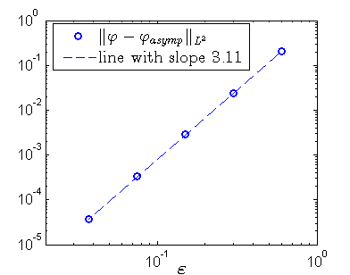
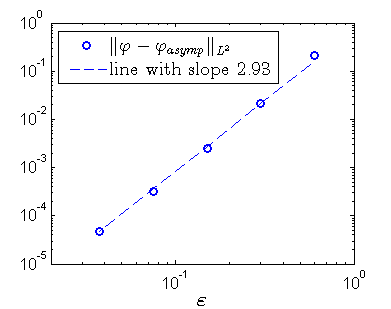
Figure 3 shows the continuation diagram (in the $(\omega,\|\varphi\|_{L^{2}({\mathbb{P}}^{2})})$-plane) of the nonlinear Bloch waves bifurcating from $\omega_{*}$ for $\sigma=-1$ and $\sigma=1$, the asymptotic curves $(\omega_{*}+\Omega\varepsilon^{2},\varepsilon|A|)$ for $\varepsilon\geq 0$, and the error between the two in the log-log scale. The observed convergence rate is 3.11, in agreement with Theorem 1.

Figure 3. Left: Bifurcation diagram in the $(\omega,\|\varphi\|_{L^{2}({\mathbb{P}}^{2})})$-plane for example A: $N=1$, $k_{*}=(\tfrac{1}{2},\tfrac{1}{2})$. Dashed lines: approximation $\|\varphi\|_{L^{2}({\mathbb{P}}^{2})}\sim|A|\sqrt{(\omega-\omega_{*})/\Omega}$ with $\Omega=\sigma=\pm 1$. Curves bifurcating to the left/right of $\omega_{*}$ are for $\sigma=\mp 1$, respectively. The spectrum $\sigma(-\Delta+V)$ is plotted on the horizontal axis. Right: Error for $\sigma=-1$, where $\varphi_{asymp}:=\varepsilon A\xi_{1}(x,k_{*})$.

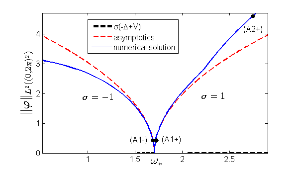
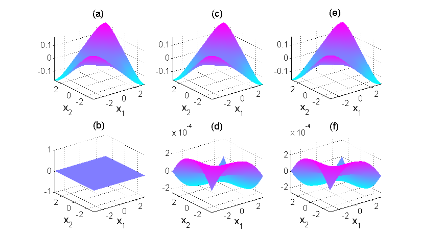
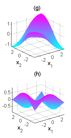
In Fig. 4 we plot profiles $\varphi$ and the asymptotic approximation $\varepsilon A\xi_{1}(x,k_{*})$ at $\omega=\omega_{*}+\varepsilon^{2}\Omega$ with $\varepsilon\approx 0.12$, i.e. close to the bifurcation point, see points (A1-) and (A1+) in Fig. 3, and $\varphi$ at $\omega\approx 2.75$ for $\sigma=1$, i.e. far from the bifurcation, cf. point (A2+). The asymptotic approximation is real since the Bloch wave $\xi_{1}(x,k_{*})$ has been selected real. This is possible as $k_{*}$ is one of the high symmetry points $\Gamma,X,M$.

Figure 4. Nonlinear Bloch waves for example A. (a) and (b): real and imaginary part of the approximation $\varepsilon A\xi_{1}(x,(1/2,1/2))$ at $\varepsilon=0.12$; (c) and (d): real and imag. part of $\varphi$ at (A1-) in Fig. 3; (e) and (f): real and imag. part of $\varphi$ at (A1+) ($\sigma=1$ and $\omega=\omega_{*}+\sigma\varepsilon^{2}$); (g) and (h): real and imag. part of $\varphi$ at (A2+)

7.2. Numerical Examples for $N=2$.

We present computations for two consistent examples with $N=M=2$, cf. §6.2 (a), where the ACMEs (6.3) are valid. In example B we choose $\omega_{*}\in\partial\sigma(-\Delta+V)$ and in example C we take $\omega_{*}\in\text{int}(\sigma(-\Delta+V))$.

Example B: We choose $k_{*}^{(1)}=(1/2,0),k_{*}^{(2)}=(0,1/2),\partial\sigma(-\Delta+V)\ni\omega_{*}=\omega_{2}(k_{*}^{(1)})=\omega_{2}(k_{*}^{(2)})\approx 2.035$, see point $(B)$ in Fig. 1. Choosing real Bloch waves $\xi_{2}(\cdot,k^{(1)}_{*}),\xi_{2}(\cdot,k^{(2)}_{*})$ (possible due to the real boundary conditions in (1.5)), we obtain

$$\mu_{1111}=\mu_{2222}=\|\xi_{2}(\cdot,k^{(1)}_{*})\|_{L^{4}({\mathbb{P}})}^{4}\approx 0.0901,$$

$$\mu_{2121}=\mu_{1221}=\int_{{\mathbb{P}}^{2}}\xi_{2}(x,k^{(1)}_{*})^{2}\xi_{2}(x,k^{(2)}_{*})^{2}dx\approx 0.003,$$

where the equalities between the $\mu$ coefficients follow by the symmetry $\xi_{2}((x_{1},x_{2}),k^{(1)}_{*})=\xi_{2}((x_{2},x_{1}),k^{(1)}_{*})$ and the fact that real Bloch waves $\xi_{2}(x,k^{(1)}_{*}),\xi_{2}(x,k^{(2)}_{*})$ have been chosen.

The resulting values of $|A_{1}|$ and $|A_{2}|$ are $|A_{1}|=|A_{2}|\approx 3.17567$ and in order to satisfy reversibility, we choose zero phases, such that

$$A_{1}=A_{2}\approx 3.17567.$$

The non-degeneracy condition is satisfied as our computation of the eigenvalues of ${\bf\hat{J}}$ produces

$$\lambda_{1}\approx-0.1223,\ \lambda_{2}=0,\ \lambda_{3}\approx 1.6332,\ \lambda_{4}=2.$$

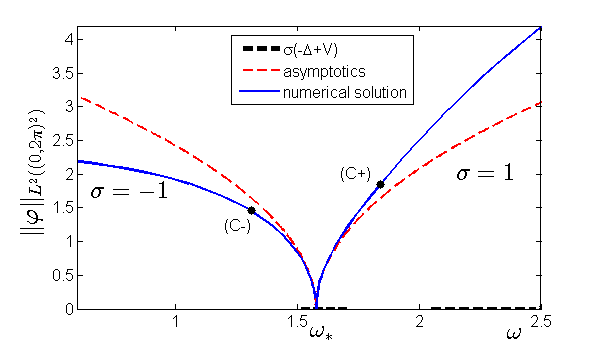
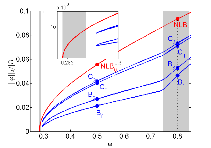
The continuation diagram in Fig. 5 plots the families of nonlinear Bloch waves bifurcating from $\omega_{*}$ for $\sigma=-1$ and $\sigma=1$, the asymptotic curves $(\omega_{*}+\Omega\varepsilon^{2},\varepsilon\|\sum_{j=1}^{2}A_{j}\xi_{2}(\cdot,k^{(j)}_{*})\|_{L^{2}({\mathbb{P}}^{2})})$ for $\varepsilon\geq 0$, and the $\varepsilon-$convergence of the approximation error for this case.

Figure 5. Left: Bifurcation diagram in the $(\omega,\|\varphi\|_{L^{2}({\mathbb{P}}^{2})})$-plane for example B: $N=2,k_{*}^{(1)}=(1/2,0),k_{*}^{(2)}=(0,1/2)$. Full lines: numerically computed solution $\varphi$; dashed lines: asymptotic approximation $\|\varphi\|_{L^{2}({\mathbb{P}}^{2})}\sim\sqrt{(\omega-\omega_{*})/\Omega}\|\sum_{j=1}^{2}A_{j}\xi_{2}(\cdot,k^{(j)}_{*})\|_{L^{2}({\mathbb{P}}^{2})}$ with $\Omega=\sigma=\pm 1$. Right: error for $\sigma=-1$, $\varphi_{asymp}:=\varepsilon\sum_{j=1}^{2}A_{j}\xi_{2}(x,k_{*}^{(j)})$.

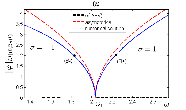
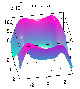
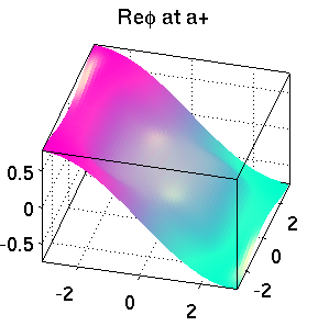
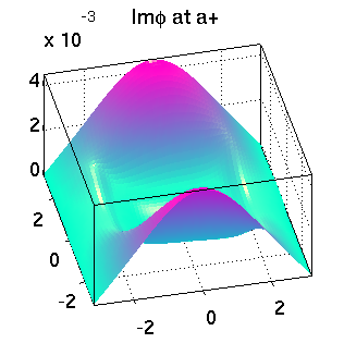
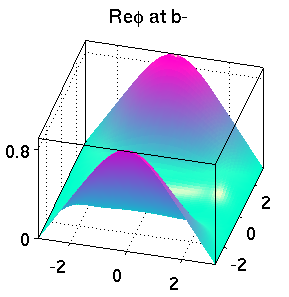
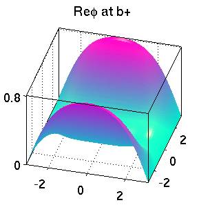
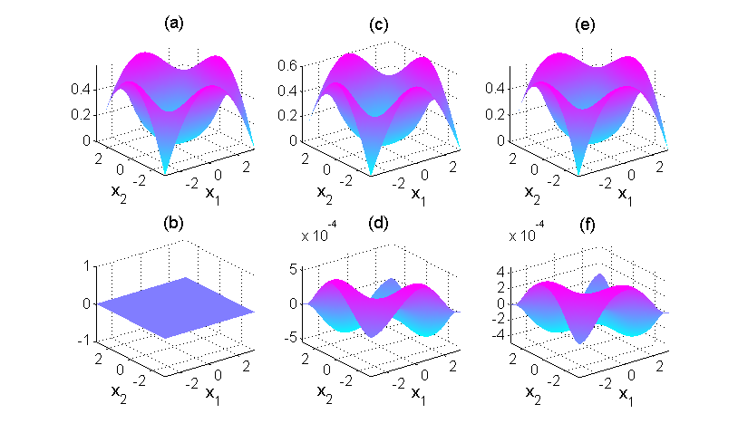
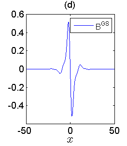
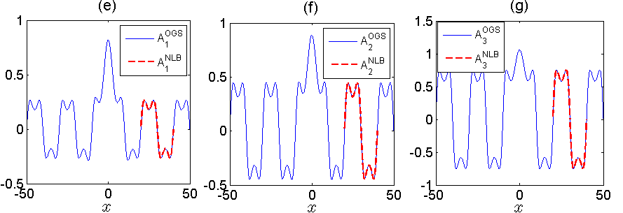
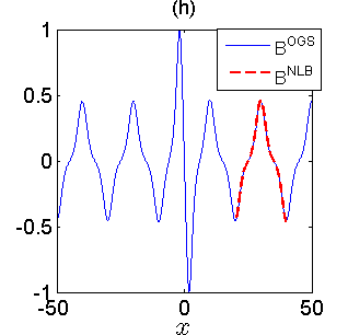
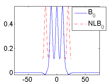
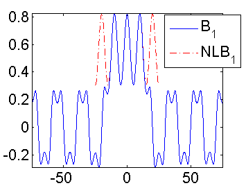
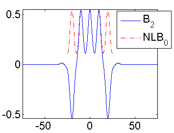
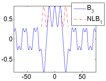
The solutions $\varphi$ at the points (B-), i.e. $\omega=1.8304$, and (B+), i.e. $\omega=2.2392$, marked in Fig. 5 are plotted in Fig. 6 together with the asymptotic approximation $\varepsilon\sum_{j=1}^{2}A_{j}\xi_{2}(x,k_{*}^{(j)})$ at $\omega=\omega_{*}+\varepsilon^{2}\Omega$ with $\varepsilon\approx 0.452\approx\sqrt{\omega_{*}-1.8304}\approx\sqrt{2.2392-\omega_{*}}$. Despite the large value of $\varepsilon$ the asymptotic approximation is relatively good.

Figure 6. Nonlinear Bloch waves for example B. (a) and (b): real and imaginary part of the asymptotic approximation $\varepsilon\sum_{j=1}^{2}A_{j}\xi_{2}(x,k_{*}^{(j)})$ at $\varepsilon=0.452$; (c) and (d): real and imaginary part of $\varphi$ at (B-) in Fig. 5, i.e. for $\sigma=-1$ and $\omega=\omega_{*}+\sigma\varepsilon^{2}$; (e) and (f): real and imaginary part of $\varphi$ at (B+) in Fig. 5, i.e. for $\sigma=1$ and $\omega=\omega_{*}+\sigma\varepsilon^{2}$.

Example C: Finally, we take $k_{*}^{(1)}=(1/4,1/4),k_{*}^{(2)}=(-1/4,-1/4),\text{int}(\sigma(-\Delta+V))\ni\omega_{*}=\omega_{1}(k_{*}^{(1)})=\omega_{1}(k_{*}^{(2)})\approx 1.576$, see Point (C) in Fig. 1. Fixing the free complex phase of the Bloch waves by setting $\text{Im}(\xi_{1}((0,0),k_{*}^{(1)})=\text{Im}(\xi_{1}((0,0),k_{*}^{(2)})=0$, we obtain

$$\mu_{1111}=\mu_{2222}=\mu_{1221}=\|\xi_{1}(\cdot,k^{(1)}_{*})\|_{L^{4}({\mathbb{P}})}^{4}\approx 0.0526,$$

$$\mu_{2121}=\int_{{\mathbb{P}}^{2}}\xi_{1}(x,k_{*}^{(2)})^{2}\overline{\xi_{1}(x,k_{*}^{(1)})}^{2}dx\approx 0.0412.$$

The identities $\mu_{1111}=\mu_{2222}=\mu_{1221}$ follow from $\xi_{1}(x,k_{*}^{(2)})=\overline{\xi_{1}(x,k_{*}^{(1)})}$, and $\mu_{2121}\in\mathbb{R}$ follows because $\text{Im}(\xi_{1}(x,k_{*}^{(1,2)}))$ happen to be antisymmetric in the $x_{1}=x_{2}$ direction. The resulting values of $A_{1}$ and $A_{2}$ (once again selected real due to $\mu_{2121}\in\mathbb{R}$) are

$$A_{1}=A_{2}\approx 2.242.$$

Also here the non-degeneracy condition is satisfied as our computation of the eigenvalues of ${\bf\hat{J}}$ produces $\lambda_{1}\approx-0.9427,\ \lambda_{2}\approx-0.828,\ \lambda_{3}=0,\ \lambda_{4}=2.$

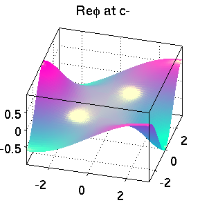
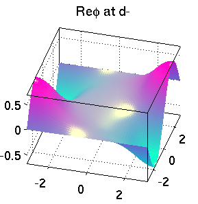
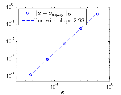
The continuation diagram from $\omega_{*}$ for $\sigma=-1$ and $\sigma=1$ and an error plot for $\sigma=-1$ are in Fig. 7, and the solutions $\varphi$ at the points (C$\mp$) with $\omega=1.31,\omega=1.842$, are in Fig. 8 together with the asymptotic approximation $\varepsilon\sum_{j=1}^{2}A_{j}\xi_{1}(x,k_{*}^{(j)})$ at $\omega=\omega_{*}+\varepsilon^{2}\Omega$ with $\varepsilon\approx 0.516\approx\sqrt{\omega_{*}-1.31}\approx\sqrt{1.842-\omega_{*}}$.

Figure 7. Bifurcation diagram in the $(\omega,\|\varphi\|_{L^{2}({\mathbb{P}}^{2})})$-plane and error for $\sigma=-1$ for example C: $N=2,k_{*}^{(1)}=(1/4,1/4),k_{*}^{(2)}=-k_{*}^{(1)}$.

Figure 8. Nonlinear Bloch waves for example C. (a): the approximation $\varepsilon\sum_{j=1}^{2}A_{j}\xi_{1}(x,k_{*}^{(j)})$ with $\varepsilon=0.516$; (b) and (c): $\varphi$ at (C-) and (C+) resp. in Fig. 7. In (b) $\sigma=-1$ and $\omega=\omega_{*}-\varepsilon^{2}\approx 1.31$ and in (c) $\sigma=1$ and $\omega=\omega_{*}+\varepsilon^{2}\approx 1.842$.

8. Gap solitons, out–of–gap solitons, and tNLBs

NLBs play an important role in the bifurcation structure of many other solutions of (1.2). As the numerical computations below suggest, when solutions with decaying tails are continued from spectral gaps into spectrum of $-\Delta+V$, they delocalize as the tails become oscillatory with the oscillation structure agreeing with a certain NLB. This puts NLBs in a strong connection with other prominent solutions of (1.2).

8.1. 1D simulations

We first consider (1.2) in 1D with $V(x)=\sin^{2}(\frac{\pi x}{10})$, which is a standard choice in 1D. See Fig. 9(a) for the band–structure, which shows the gaps $(s_{2},s_{3})$ and $(s_{4},s_{5})$. The first five spectral edges are, approximately,

$$s_{1}\approx 0.2832,\quad s_{2}\approx 0.2905,\quad s_{3}\approx 0.7468,\quad s_{4}\approx 0.8434,\quad s_{5}\approx 1.0568.$$

For suitable $\sigma=\pm 1$, so called gap solitons bifurcate from the edges into a gap [1, 3, 30]. We display here gap soliton families bifurcating for $\sigma=1$ to the right from edge $s_{2}$ and for $\sigma=-1$ to the left from $s_{3}$. To study these numerically, we consider (1.2) on a large domain $x\in(-100,100)$ with Neumann boundary conditions, and obtain the bifurcation diagram in Fig. 9(b), where moreover we restrict to real solutions.

Figure 9. Panel (a): the band–structure for $V(x)=\sin^{2}(\frac{\pi x}{10})$; (b): a bifurcation diagram of GS and NLBs for (1.2) in 1D, $\sigma=1$. (c) and (d): plots of the GS at $A^{\text{GS}}$ and $B^{\text{GS}}$ resp.; (e)-(h): OGS and NLB at the remaining marked points.

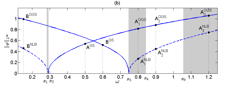
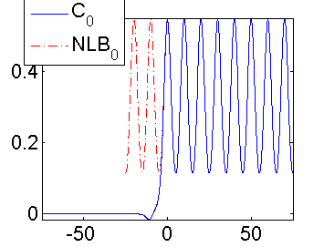
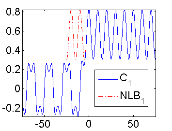
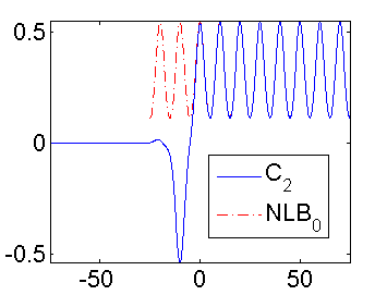
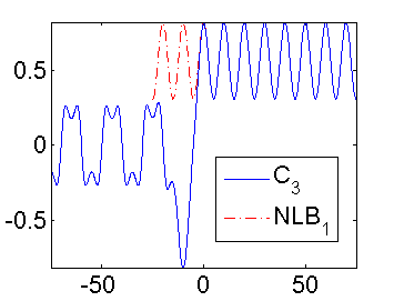
The gap solitons can be continued in $\omega$ well into the gap. In fact, numerically they can also be continued into the next spectral band (and even further into higher gaps and bands), where they are called out–of-gap solitons (OGS) [41, 24]. During this continuation the tails of the OGS pick up the oscillations from the NLB that bifurcates at the first gap edge, where the continuation family enters the spectrum, i.e., the $A$ branch of OGS picks up the oscillations from the NLB branch $A^{\text{NLB}}$ that bifurcates at $s_{3}$ to the right. Moreover, the numerics then show that the tails of the OGS are given by $A^{\text{NLB}}$ for all $\omega>s_{3}$. The same can be observed for the $B$-family, where the OGS tails are given by $B^{\text{NLB}}$ for all $\omega<s_{2}$. Thus, an OGS is a homoclinic orbit to a NLB.

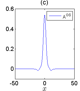
Besides GSs the NLB play a role in the delocalization of many other solutions. In Fig. 10 we show two other solution branches for illustration. The $B$ branch is an example of a so called truncated NLB (tNLB), [4, 38, 42]. Point $B_{0}$ at $\omega=0.5$ on that branch is obtained from using

(8.1) $$\varphi_{IG}(x)=a{\rm sech}(x^{2}/w),\quad a=0.5,w=50,$$

as an initial guess for a Newton–loop for (1.2). It is homoclinic to $0$ and composed of three periods of the NLB bifurcating from $s_{1}$ in the middle. That is why such solutions are called truncated NLBs. By varying, e.g., $w$ in (8.1), we can in fact produce tNLBs composed of any number of periods of the NLB.

Figure 10. Big panel: bifurcation diagram of first NLB and example tNLBs and heteroclinics for $V(x)=\sin^{2}(\frac{\pi x}{10})$, $\sigma=1$; spectral bands in grey. For the $B$ (tNLB) and $C$ (heteroclinic) branches we continue from $\omega=0.5$ in the positive and negative $\omega$ direction. For the negative $\omega$–directions we obtain folds close to $s_{2}$, cf. the inset. The NLB branch bifurcates from $s_{1}$. Smaller panels: example plots, where the red dash-dotted line indicates the $s_{1}$–NLB at the respective $\omega$–values. The tails of the tNLBs, and the zero–level of the heteroclinic, pick up the $s_{3}$–NLB when entering the second band.

An important feature of tNLBs is that they do not bifurcate from $0$, in contrast to the GS. In fact, as a tNLB approaches the gap edge next to the $\omega$ value where its building–block NLB bifurcates, it turns around while picking up a negative copy of the pertinent NLB. See also [37] for a further discussion (in 2D). On the other hand, tNLBs behave quite similarly to GS upon continuation through the other gap–edge: the tails again pick up the NLB bifurcating at the edge (the tNLBs in Fig. 10 pick up the NLB family bifurcating from $s_{3}$ in Fig. 9), and afterward can be continued to arbitrarily large $\omega$ as homoclinics to these NLBs, still being close to the original NLB in the middle. For these delocalized tNLBs we suggest the acronym dtNLBs.

Finally, as there are “arbitrarily long” tNLBs, it is not surprising that there also exist heteroclinics between $0$ and NLBs. Upon continuation in $\omega$ these essentially behave like tNLBs, see the $C$ branch in Fig. 10 for an example.

A rigorous analysis of OGS, tNLBs, dtNLBs, and the above heteroclinics remains an intriguing open problem, even in 1D. For the 1D case with narrow gaps a system of first order differential coupled mode equations for the envelopes of the linear gap edge Bloch waves is derived in [41]. Under suitable conditions, this system has spatial homoclinic orbits to nonzero fixed points, which thus corresponds to dtNLBs or OGS. However, presently it is not clear how to make this analysis rigorous. In [24] some explicit OGS solutions are given for the case of a 1D discrete NLS. Concerning tNLBs, [43] gives so called composition relations, which however are rather heuristic. Delocalized (or generalized) solitary waves also occur in other nonlinear equations, in particular from fluid dynamics. See, e.g., [7, Chapters 1 and 6.4] for a review, and a guide to the literature for rigorous existence proofs, for instance [35] for the case of the fifth-order KdV equation. The solutions studied in this literature, however, typically have exponentially small tails, which is different from our OGS and dtNLBs, where the amplitude of the tails is that of the NLBs, i.e. $O(\varepsilon^{1/2})$ in the bifurcation parameter $\varepsilon$ as given by (2.1).

8.2. 2D simulations

In 2D similar effects as in Figs. 9 and 10 occur, but the solution structure becomes much richer, also qualitatively. For instance, since in 1D the pertinent NLS amplitude equation is scalar, there typically is only one GS bifurcating at some $s_{j}$ (modulo phase invariance, and on–site or off-site effects, see [30]). In 2D, in many cases the GS are described by systems of NLS equations, see [15], and there may be various different GSs. Moreover, while typically in 1D different tNLBs at fixed $\omega$ only differ in the number of NLB periods, and the number and arrangements of “ups” and “downs”, in 2D we can easily produce qualitatively different tNLBs. Accordingly, in the references already cited, in particular [37], various families of 2D tNLBs have been studied, with focus on the fold structure near one of the gap-edges.

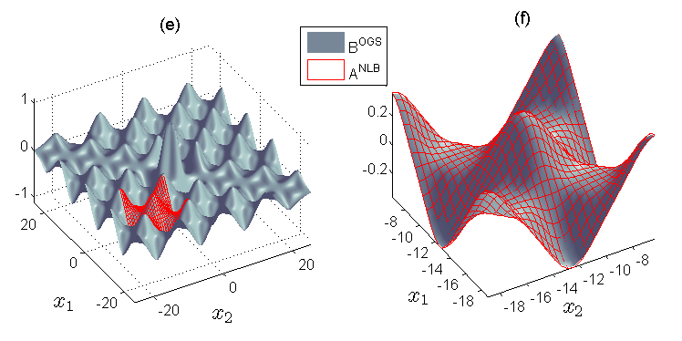
However, the continuation of either tNLBs or GSs into the other spectral band seems to be much less studied, but see also [39]. Here we restrict ourselves to just illustrating the continuation of two (real) families of GS to OGS. We return to the potential (1.4), and in Fig. 11 continue the $\sigma=\pm 1$ GS from the first gap into the respective other spectral band. Numerically we again use a large domain $x\in(-40\pi,40\pi)^{2}$ with Neumann boundary conditions. For the GS these boundary conditions hardly matter, but the way in which the tails pick up NLBs as the GS enter the spectral bands does significantly depend on the boundary conditions, as should be expected. For instance, in (b) we find dislocations in the tail patterns along the coordinate axes, and in (e) along one of the diagonals. Numerically, these dislocations strongly depend on the chosen domain size and boundary conditions. Nevertheless, in all cases considered the tails of the GS again pick up a pertinent NLB in large parts of the domains. Figure 11 just gives two illustrations.

Figure 11. Continuation of 2D–GS from the first spectral gap to OGS, see the text for comments.

Note that in 2D there is typically a number of NLB families bifurcating from a given point in the spectrum, cf. Theorem 1 with $N>1$. At $\omega=s_{3}$ the level set of the band structure is $\{(1/2,0),(0,1/2)\}$, i.e. to capture at least all the NLBs predicted by Theorem 1 to bifurcate from $s_{3}$, we must take $N=2$. The resulting ACMEs are (6.3). The NLB family $B$ in Fig. 11, which happens to describe the oscillations in $A^{\text{OGS}}$, has $A_{1}=A_{2}\in\mathbb{R}$. In general it is not clear how to choose the correct solution of ACME which matches the tail oscillations in a given OGS in $d$D with $d\geq 2$.

8.3. Remarks on stability of NLBs, GS, tNLBs, and OGS and dtNLBs

Dynamic stability of GS, NLBs, (localized and delocalized) tNLBs and OGS is an important but widely open question. Previous work, mostly based on numerics and formal asymptotics, include the following: In [22] and [6] it is shown that, so called, on-site GSs in 1D are spectrally stable while off-site ones are unstable. [31] and [40] show that 2D GSs near the spectral edge from which they bifurcate, are spectrally unstable but can be stable further away from the edge. Next, [20] gives numerics and formal asymptotics that indicate that GS near the middle of (narrow) band gaps may be unstable due to a four wave mixing with the gap edge NLBs. In [25] it is discussed that modulational instability of 1D NLBs bifurcating from gap edges into the gap can lead to the formation of GS, while NLBs bifurcating from the edge into the spectrum are stable. Some semi-analytical results on the stability of NLB at the bottom of the band structure are given in [9], where, together with the secondary bifurcations from NLBs, exchange of stability results are derived under some assumptions, and numerical justifications and comparisons to numerical time–integration are given. Regarding tNLBs, in [38] it is shown numerically that tNLB of the type $B_{0}$ in Fig. 10, i.e., consisting of arbitrary many periods of NLBs of the same parity, can be stable, while tNLB on the upper branch, consisting of up and down copies of the basic NLB, are generically unstable.

Here we report some stability results from numerical time integration of (1.1) using a Fourier split-step method. We plug $\psi(t,x)={\rm e}^{{\rm i}\omega t}\varphi(t,x)$ into (1.1) to obtain

(8.2) $${\rm i}\partial_{t}\varphi=\Delta\varphi-(V(x)-\omega)\varphi-\sigma|\varphi|^{2}\varphi.$$

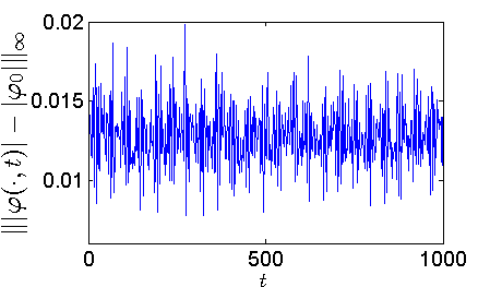
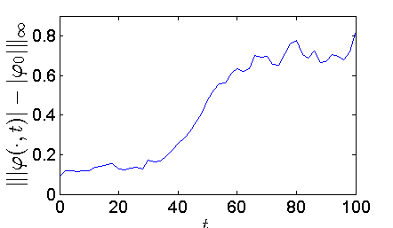
Since (1.1) is Hamiltonian, we can at best obtain spectral stability (but not linearized stability) from linearization of (8.2) around a steady state $\varphi(x,t)=\varphi_{0}(x)$ of interest (NLB, GS, tNLB etc). As initial conditions we choose random perturbations of the steady state $\varphi_{0}$, with perturbation amplitude 0.1 relative to the amplitude of $\varphi_{0}$. These perturbations yield a phase evolution, and thus here we concentrate on the solution shape, i.e., we plot the supremum error $\||\varphi(\cdot,t)|-|\varphi_{0}(\cdot)|\|_{\infty}$ of the modulus. This should provide an indication regarding stability of the solutions at hand and motivate further stability studies. Our numerical accuracy was checked by using smaller time steps without visible changes of results, by comparison with a semi–implicit time stepping, and we checked that $\|\varphi\|_{L^{2}}$ was conserved up to 6 digits over the rather long time intervals needed in some cases to detect instabilities.

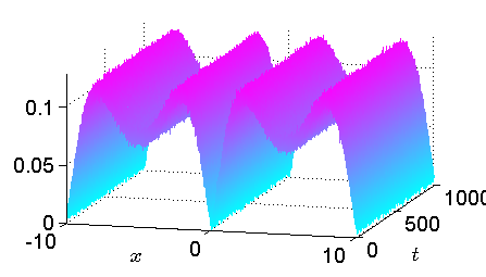
We mostly focus on 1D, and start with the NLBs. In order to draw a connection between stability of NLBs and OGSs, we restrict ourselves to NLBs bifurcating at gap edges in Fig. 9. We choose the periodicity cell $x\in\Omega=(-10,10)$ for $\varphi$, which corresponds to wave-vectors $k=0$ and $k=1/2$. However, the results appear to be the same for larger domains, i.e., if we observe instabilities, then they are w.r.t. the same spatial period. Below we use the symbol $s_{n}\pm$ to denote the NLB families bifurcating from a spectral edge $s_{n}$ to the right and left respectively.

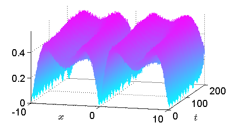
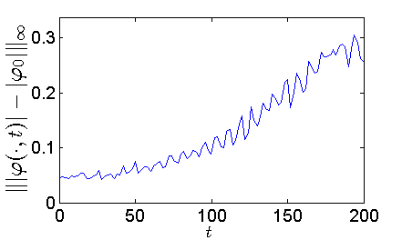
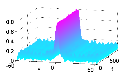
Panels (a)-(d) in Fig. 12 are for the NLB branch $s_{3}+$ in Fig. 9 for $\sigma=1$. As an example in (a),(b) we choose $\omega=0.76$ and observe a stable evolution up to $t=1000$. In (c), (d) the NLB at $\omega=0.9$, i.e. further away from the bifurcation edge, is shown to be unstable. An analogous situation occurs for the $s_{2}-$ family of NLB for $\sigma=-1$. It appears stable for $\omega\in(0.2,s_{2})$ and unstable for $\omega<0.2$.

(a) NLB $s_{3}+,\omega{=}0.76$	(b) NLB $s_{3}+,\omega{=}0.76$	(c) NLB $s_{3}+,\omega{=}0.9$	(d) NLB $s_{3}+,\omega{=}0.9$
$|\varphi|$	amplitude error	$|\varphi|$	amplitude error

(e) OGS $s_{2}+,\ \omega{=}0.76$	(f) OGS $s_{2}+,\ \omega{=}0.76$	(g) OGS $s_{2}+,\ \omega{=}0.9$	(h) OGS $s_{2}+,\ \omega{=}0.9$
$|\varphi|$	amplitude error	$|\varphi|$	amplitude error

Figure 12. Numerical integration of (8.2) with initial data as random 10% perturbations of the indicated NLB in (a)-(d) and OGS in (e)-(h). The NLB-branch $s_{3}+$ appears stable at bifurcation and unstable otherwise. The OGS family $s_{2}+$ entering the spectrum at $\omega=s_{3}$ seems to inherit the (in)stability of the NLB.

Our tests suggest that similar stability results (stability near the bifurcation edge and instability otherwise) hold also for other NLB branches bifurcating into the spectral bands in Fig. 9. The stability near the bifurcation edge is in agreement with [25]. The loss of stability of NLB away from a neighborhood of the bifurcation point is presumably due to a secondary “loop” bifurcation as discussed in [9].

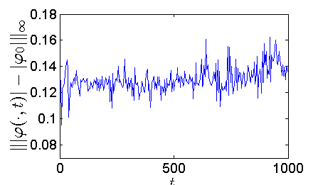
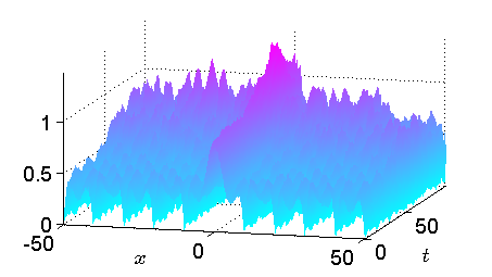
Given the results on the NLBs from Fig. 12 (a)-(d), we may expect that the OGS with tails picking up the $s_{3}+$ NLBs at $s_{3}$ inherit the (in)stability from the NLBs $s_{3}+$ NLBs and hence is stable at $\omega=0.76$ and unstable at $\omega=0.9$. This is, indeed, observed in Fig. 12 (e)-(h). Note that one does not expect any instability from the GS “component” of the OGS since we work with on-site GSs, which have been reported in [22] and [6] to be stable.

Next, the NLB branch $s_{1}+$ bifurcating from $s_{1}$ to the right for $\sigma=1$ is stable throughout the first band and the first gap. Thus, another relevant question is whether the associated tNLBs inherit this stability of their building blocks. In accordance with, e.g., [38], this is the case for tNLB consisting of copies of NLBs with the right parity, i.e., only up or only down copies of $s_{1}+$ NLBs; see for instance the tNLBs $B_{0}$ and $C_{0}$ from Fig. 10. In a next step we then studied the stability of dtNLBs obtained from the continuation of such tNLBs across the $s_{3}$ gap edge. This is in complete agreement with the stability of OGS, i.e., the dtNLBs obtained from $B_{0},C_{0}$ (see $B_{1},C_{1}$ in Fig. 10) are stable for small $\omega{-}s_{3}{>}0$ but become unstable for larger $\omega{-}s_{3}$. On the other hand, we found that tNLBs consisting of up and down copies of NLBs (e.g., $B_{2}$, $C_{2}$ in Fig. 10) are unstable, as in [38]. For instance, for $C_{2}$ the leading down NLB is first converted into an up NLB, and then a defect wanders to the right.

In 2D, the NLBs from Fig. 2 all appear modulationally unstable, with however very long transients before the instability sets in for the branches bifurcating at smaller $\omega$, and this also holds for the other NLBs, for instance given in §7.2. Moreover, the 2D-GS are expected to be unstable near bifurcation, but may become stable in the middle of gaps, see [23] for rigorous results in the semi-infinite gap, and [40, §6.4] for further heuristics. This agrees with our numerics, where e.g., solutions on the $A^{\text{GS}}$ branch from Fig. 11 are numerically unstable for $\omega<1.8$, then stable up to $\omega=s_{3}$. However, the OGS for $\omega>s_{3}$ with tails containing $B^{\text{NLB}}$ NLBs is clearly unstable numerically.

Thus, besides analytical results regarding the existence and stability of tNLBs, OGS and (d)tNLB, an interesting open problem is whether in 2D there exist potentials V such that

1. (1.1) has stable GS;

2. (1.1) has stable NLBs bifurcating from gap edges;

3. putting (1) and (2) together: (1.1) has stable OGS.

References

- [1] A. B. Aceves. Optical gap solitons: Past, present, and future; theory and experiments. Chaos, 10:584–589, 2000.
- [2] R.A. Adams and J.J.F. Fournier. Sobolev Spaces. Pure and Applied Mathematics. Elsevier Science, 2003.
- [3] G. P. Agrawal. Nonlinear Fiber Optics. Academic Press, 2001.
- [4] T.J. Alexander, E. A. Ostrovskaya, and Yu. S. Kivshar. Self-trapped nonlinear matter waves in periodic potentials. PRL, 96:040401–4, 2006.
- [5] Chr. Bersch, G. Onishchukov, and U. Peschel. Optical gap solitons and truncated nonlinear Bloch waves in temporal lattices. Phys. Rev. Lett., 109:093903, 2012.
- [6] E. Blank and T. Dohnal. Families of surface gap solitons and their stability via the numerical Evans function method. SIAM Journal on Applied Dynamical Systems, 10(2):667–706, 2011.
- [7] J. P. Boyd. Weakly nonlocal solitary waves and beyond-all-orders asymptotics, volume 442 of Mathematics and its Applications. Kluwer Academic Publishers, Dordrecht, 1998.
- [8] K. Busch, G. Schneider, L. Tkeshelashvili, and H. Uecker. Justification of the nonlinear Schrödinger equation in spatially periodic media. Z. Angew. Math. Phys., 57:905–939, 2006.
- [9] M. Coles and D. Pelinovsky. Loops of energy bands for bloch waves in optical lattices. Studies in Applied Mathematics, 128(3):300–336, 2012.
- [10] M. Cristiani, O. Morsch, J.H. Müller, D. Ciampini, and E. Arimondo. Experimental properties of Bose-Einstein condensates in one-dimensional optical lattices: Bloch oscillations, Landau-Zener tunneling, and mean-field effects. Phys. Rev. A, 65(6):063612, 2002.
- [11] T. Dohnal. Traveling solitary waves in the periodic nonlinear Schrödinger equation with finite band potentials. SIAM Journal on Applied Mathematics, 74(2):306–321, 2014.
- [12] T. Dohnal, D.E. Pelinovsky, and G. Schneider. Coupled-mode equations and gap solitons in a two-dimensional nonlinear elliptic problem with a separable periodic potential. J. Nonlin. Sci., 19:95–131, 2009.
- [13] T. Dohnal, J. Rademacher, H. Uecker, and D. Wetzel. pde2path 2.0: multi-parameter continuation and periodic domains. In H. Ecker, H. Steindl, and S. Jakubek, editors, ENOC 2014 - Proceedings of 8th European Nonlinear Dynamics Conference.
- [14] T. Dohnal, J. Rademacher, H. Uecker, and D. Wetzel. pde2path 2.0 user manual. 2014. See www.staff.uni-oldenburg.de/hannes.uecker/pde2path.
- [15] T. Dohnal and H. Uecker. Coupled mode equations and gap solitons for the 2d Gross-Pitaevskii equation with a non-separable periodic potential. Physica D, 238(9-10):860–879, 2009.
- [16] M.S.P. Eastham. Spectral Theory of Periodic Differential Equations. Scottish Academic Press, Edinburgh London, 1973.
- [17] N.K. Efremidis, J. Hudock, D.N. Christodoulides, J.W. Fleischer, O. Cohen, and M. Segev. Two-dimensional optical lattice solitons. Phys. Rev. Lett., 91:213906, 2003.
- [18] C.L. Fefferman and M.I. Weinstein. Honeycomb lattice potentials and Dirac points. J. Amer. Math. Soc., 25(4):1169–1220, 2012.
- [19] Gadi Fibich. The nonlinear Schrödinger equation, volume 192 of Applied Mathematical Sciences. Springer, Cham, 2015. Singular solutions and optical collapse.
- [20] E. Gaizauskas, A. Savickas, and K. Staliunas. Radiation from band-gap solitons. Optics Communication, 285(8):2166–2170, 2012.
- [21] L. Hörmander. The Analysis of Linear Partial Differential Operators III: Pseudo-Differential Operators. Springer, 2007.
- [22] G. Hwang, T.R. Akylas, and J. Yang. Gap solitons and their linear stability in one-dimensional periodic media. Physica D: Nonlinear Phenomena, 240(12):1055 – 1068, 2011.
- [23] B. Ilan and M. I. Weinstein. Band-edge solitons, nonlinear Schrödinger/Gross-Pitaevskii equations, and effective media. Multiscale Modeling & Simulation, 8(4):1055–1101, 2010.
- [24] B. Johanson, K. Kirr, A. Kovalev, and L. Kroon. Gap and out-gap solitons in modulated systems of finite length: exact solutions in the slowly varying envelope limit. Phy. Scr., 83:065005, 2011.
- [25] V. V. Konotop and M. Salerno. Modulational instability in Bose-Einstein condensates in optical lattices. Phys. Rev. A, 65:021602(R), 2002.
- [26] P. J. Y. Louis, E. A. Ostrovskaya, C. M. Savage, and Yu. S. Kivshar. Bose-Einstein condensates in optical lattices: Band-gap structure and solitons. Phys. Rev. A, 67:013602–9, 2003.
- [27] R. S. Maier. Lamé polynomials, hyperelliptic reductions and Lamé band structure. Phil. Trans. R. Soc. A, 366:1115–1153, 2008.
- [28] Z. Mei. Numerical bifurcation analysis for reaction-diffusion equations, volume 28 of Springer Series in Computational Mathematics. Springer-Verlag, Berlin, 2000.
- [29] L. Nirenberg. Topics in Nonlinear Functional Analysis. Courant Institute of Mathematical Sciences. Courant Institute of Mathematical Sciences, 1974.
- [30] D. E. Pelinovsky. Localization in periodic potentials, volume 390 of London Mathematical Society Lecture Note Series. Cambridge University Press, Cambridge, 2011.
- [31] Z. Shi, J. Wang, Z. Chen, and J. Yang. Linear instability of two-dimensional low-amplitude gap solitons near band edges in periodic media. Phys. Rev. A, 78:063812, Dec 2008.
- [32] Z. Shi and J. Yang. Solitary waves bifurcated from Bloch-band edges in two-dimensional periodic media. Phys. Rev. E, 75:056602, 2007.
- [33] A.A. Sukhorukov and Y.S. Kivshar. Nonlinear guided waves and spatial solitons in a periodic layered medium. J. Opt. Soc. Am. B, 19(4):772–781, 2002.
- [34] C. Sulem and P.-L. Sulem. The nonlinear Schrödinger equation, volume 139 of Applied Mathematical Sciences. Springer-Verlag, New York, 1999.
- [35] S. M. Sun and M. C. Shen. Exponentially small estimate for a generalized solitary wave solution to the perturbed K-dV equation. Nonlinear Anal., 23(4):545–564, 1994.
- [36] H. Uecker, D. Wetzel, and J. Rademacher. pde2path – a Matlab package for continuation and bifurcation in 2D elliptic systems. NMTMA (Numerical Mathematics : Theory, Methods, Applications), 7:58–106, 2014.
- [37] J. Wang and J. Yang. Families of vortex solitons in periodic media. Phys. Rev. A, 77:033834, 2008.
- [38] J. Wang, J. Yang, T.J Alexander, and Yu. S. Kivshar. Truncated-Bloch-wave solitons in optical lattices. Phys. Rev. A, 79:043610, 2009.
- [39] J. Yang. Fully localized two–dimensional embedded solitons. Phys. Rev. A, 82:053828, 2010.
- [40] J. Yang. Nonlinear Waves in Integrable and Nonintegrable Systems. SIAM, 2010.
- [41] A. V. Yulin and D. V Skryabin. Out-of-gap Bose-Einstein solitons in optical lattices. Phys. Rev. A, 67, 2003.
- [42] Y. Zhang, W. Liang, and B. Wu. Gap solitons and Bloch waves in nonlinear periodic systems. Phys. Rev. A, 80:063815–1, 2009.
- [43] Y. Zhang and B. Wu. Composition Relation between Gap Solitons and Bloch Waves in Nonlinear Periodic Systems. PRL, 102:093905, 2009.