On the asymptotics of Bessel functions in the Fresnel regime

Abstract

We introduce a version of the asymptotic expansions for Bessel functions $J_{\nu}(z)$, $Y_{\nu}(z)$ that is valid whenever $|z|>\nu$ (which is deep in the Fresnel regime), as opposed to the standard expansions that are applicable only in the Fraunhofer regime (i.e. when $|z|>\nu^{2}$). As expected, in the Fraunhofer regime our asymptotics reduce to the classical ones. The approach is based on the observation that Bessel’s equation admits a non-oscillatory phase function, and uses classical formulae to obtain an asymptotic expansion for this function; this in turn leads to both an analytical tool and a numerical scheme for the efficient evaluation of $J_{\nu}(z)$, $Y_{\nu}(z)$, as well as various related quantities. The effectiveness of the technique is demonstrated via several numerical examples. We also observe that the procedure admits far-reaching generalizations to wide classes of second order differential equations, to be reported at a later date.

Given a differential equation

$$y^{\prime\prime}(z)+q(z)y(z)=0$$ (1)

on a (possible infinite) interval $(a,b)$, a sufficiently smooth $\alpha$ is referred to as a phase function for (1) if $\alpha^{\prime}(z)\neq 0$ for all $z\in(a,b)$ and the pair of functions $u,v$ defined by the formulae

$$u(z)=\frac{\cos(\alpha(z))}{\left|\alpha^{\prime}(z)\right|^{1/2}},$$ (2)

$$v(z)=\frac{\sin(\alpha(z))}{\left|\alpha^{\prime}(z)\right|^{1/2}}$$ (3)

forms a basis in the space of solutions of (1). Phase functions arise from the theory of global transformations of ordinary differential equations, which was initiated in [6]; more modern discussions can be found, inter alia, in [2], [7]. Despite their long history, phase functions possess a property that appears to have been overlooked: as long as the function $q$ is non-oscillatory, the equation (1) possesses a non-oscillatory phase function. This observation in its full generality is somewhat technical, and will be reported at a later date; in this short note, we apply it to the case of Bessel’s equation

$$z^{2}\phi^{\prime\prime}(z)+z\phi^{\prime}(z)+(z^{2}-\nu^{2})\phi(z)=0\ \ \ \mbox{for all}\ \ 0<z<\infty.$$ (4)

To the authors’ knowledge, the results in this paper are new despite the long-standing interest in the phase functions associated with Bessel’s equation. The most closely related antecedents of this work appear to be [4] and [10, 11, 8]. The former uses Taylor expansions of a non-oscillatory phase function for Bessel’s equation to evaluate the Bessel functions of large arguments; and the latter three works make use of phase functions to compute zeros of Bessel functions (as well as certain other special functions).

1 Phase functions and the Kummer Equation

If $u$ and $v$ are solutions of (1) related to a $C^{3}$ function $\alpha$ via the formulae (2), (3), then

$$\tan(\alpha(z))=\frac{v(z)}{u(z)}$$ (5)

for all $z\in(a,b)$ such that $u(z)\neq 0$. We differentiate (5) in order to conclude that

$$\alpha^{\prime}(z)\sec^{2}\left(\alpha(z)\right)=\frac{u(z)v^{\prime}(z)-u^{\prime}(z)v(z)}{u^{2}(z)}$$ (6)

for all $z\in(a,b)$ such that $u(z)\neq 0$. Note that the set of zeros of any nontrivial solution of (1) is discrete, so that

$$\{z\in(a,b):u(z)\neq 0\}$$ (7)

is an open set. From (2), (3) and a straightforward calculation we conclude that

$$u(z)v^{\prime}(z)-u^{\prime}(z)v(z)=1$$ (8)

for all $z\in(a,b)$. Moreover, by applying basic trigonometric identities to (5) we obtain the formula

$$\sec^{2}\left(\alpha(z)\right)=\frac{u^{2}(z)+v^{2}(z)}{u^{2}(z)},$$ (9)

which holds for all $z\in(a,b)$ such that $u(z)\neq 0$. By combining (6), (8) and (9) we conclude that

$$\alpha^{\prime}(z)=\frac{1}{u^{2}(z)+v^{2}(z)}$$ (10)

for all $z\in(a,b)$ for which $u(z)\neq 0$. If $z\in(a,b)$ such that $u(z)=0$ but $v(z)\neq 0$, then

$$\cot(\alpha(z))=\frac{u(z)}{v(z)}.$$ (11)

Using an argument analogous to that used to derive (10) from formula (5), we conclude from (11) that (10) also holds for all $z\in(a,b)$ such that $v(z)\neq 0$. Since (8) implies that $u$ and $v$ are never simultaneously zero on the interval $(a,b)$, formula (10) in fact holds for all $z\in(a,b)$.

By differentiating (2) twice we obtain

$$u^{\prime\prime}(z)=\frac{\cos(\alpha(z))}{\sqrt{\left|\alpha^{\prime}(z)\right|}}\left(-(\alpha^{\prime}(z))^{2}-\frac{1}{2}\left(\frac{\alpha^{\prime\prime\prime}(z)}{\alpha^{\prime}(z)}\right)+\frac{3}{4}\left(\frac{\alpha^{\prime\prime}(z)}{\alpha^{\prime}(z)}\right)^{2}\right).$$ (12)

By adding $q(z)u(z)$ to both sides of (12) and making use of (2) we conclude that

$$u^{\prime\prime}(z)+q(z)u(z)=\frac{\cos(\alpha(z))}{\sqrt{\left|\alpha^{\prime}(z)\right|}}\left(q(z)-(\alpha^{\prime}(z))^{2}-\frac{1}{2}\left(\frac{\alpha^{\prime\prime\prime}(z)}{\alpha^{\prime}(z)}\right)+\frac{3}{4}\left(\frac{\alpha^{\prime\prime}(z)}{\alpha^{\prime}(z)}\right)^{2}\right).$$ (13)

Using an analogous sequence of steps, we obtain the formula

$$v^{\prime\prime}(z)+q(z)v(z)=\frac{\sin(\alpha(z))}{\sqrt{\left|\alpha^{\prime}(z)\right|}}\left(q(z)-(\alpha^{\prime}(z))^{2}-\frac{1}{2}\left(\frac{\alpha^{\prime\prime\prime}(z)}{\alpha^{\prime}(z)}\right)+\frac{3}{4}\left(\frac{\alpha^{\prime\prime}(z)}{\alpha^{\prime}(z)}\right)^{2}\right).$$ (14)

from (3). Suppose that $\alpha$ is a phase function for (1). Then

$$u^{\prime\prime}(z)+q(z)u(z)=0=v^{\prime\prime}(z)+q(z)v(z)$$ (15)

for all $z\in(a,b)$. Since

$$\cos^{2}(\alpha(z))+\sin^{2}(\alpha(z))=1,$$ (16)

the functions

$$\cos(\alpha(z))$$ (17)

and

$$\sin(\alpha(z))$$ (18)

cannot simultaneously be $0$. By combining this observation with (13), (14) and (15), we conclude that $\alpha$ satisfies the third order nonlinear differential equation

$$\left(\alpha^{\prime}(z)\right)^{2}=q(z)-\frac{1}{2}\frac{\alpha^{\prime\prime\prime}(z)}{\alpha^{\prime}(z)}+\frac{3}{4}\left(\frac{\alpha^{\prime\prime}(z)}{\alpha^{\prime}(z)}\right)^{2}$$ (19)

on the interval $(a,b)$. Suppose, on the other hand, that $\alpha$ is an element of $C^{3}\left(\left(a,b\right)\right)$ such that $\alpha^{\prime}(z)\neq 0$ for all $z\in(a,b)$, and that the function $q$ is defined by equation (19). Then (13) and (14) imply that the functions $u$ and $v$ defined via (2), (3) are solutions of (1). A straightforward calculation shows that the Wronskian

$$u(z)v^{\prime}(z)-u(z)v(z)$$ (20)

of $\{u,v\}$ is $1$, so that the pair of functions $u$, $v$ in fact forms a basis in the space of solutions of (1). We will refer to (19) as Kummer’s equation, after E. E. Kummer who studied it in [6].

Our principal interest is in the highly oscillatory case, where $q(z)$ is of the form $\gamma^{2}\widetilde{q}(z)$ with $\gamma$ a large real-valued constant and $\widetilde{q}$ a complex-valued function, so that $q(z)$ is asymptotically of the order $\gamma^{2}$. As a consequence of the Sturm comparison theorem (see, for example, [3]) solutions of (1) are necessarily highly oscillatory when $\gamma$ is large. Moreover, the form of (19) and the appearance of $\lambda$ in it suggests that phase functions for (1) will also be highly oscillatory in this regime — and most of them are. However, non-oscillatory $\alpha$ are available whenever $q$ is non-oscillatory (in an appropriate sense). In this note, we construct such an $\alpha$ in the case of Bessel’s equation.

2 A Phase function for Bessel’s equation

The Bessel function of the first kind of order $\nu$

$$J_{\nu}(z)=\left(\frac{z}{2}\right)^{\nu}\sum_{n=0}^{\infty}\frac{(-\frac{1}{4}z^{2})^{n}}{n!\ \Gamma\left(\nu+n+1\right)}$$

and the Bessel function of the second kind of order $\nu$

$$Y_{\nu}(z)=\frac{J_{\nu}(z)\cos(\nu\pi)-J_{-\nu}(z)}{\sin(\nu\pi)}$$

form a basis in the space of solutions of Bessel’s equation (4).

Bessel functions are among the most studied and well-understood of special functions. Even the standard reference books such as [1], [5] contain a wealth of information. Here, we only list facts necessary for the specific purposes of the paper; the reader is referred to [13], [1], [5] (and many other excellent sources) for more detailed information.

For arbitrary positive real $\nu$ and large values of $|z|$, the functions $J_{\nu}$, $Y_{\nu}$ possess asymptotic expansions of the form

$$J_{\nu}(z)=\sqrt{{2\over\pi\,z}}\,\cos(z-{\nu\pi\over 2}-{\pi\over 4})\,\left(1+\sum_{k=1}^{\infty}{P_{2\,k}\,(\nu)\over z^{k}}\right),$$ (21)

$$Y_{\nu}(z)=\sqrt{{2\over\pi\,z}}\,\sin(z-{\nu\pi\over 2}-{\pi\over 4})\,\left(1+\sum_{k=1}^{\infty}{Q_{2\,k}\,(\nu)\over z^{k}}\right),$$ (22)

where for each $k=1,2,\cdots$, $P_{2k},Q_{2k}$ are polynomials of order $2k$ (see, for example, [1] for exact definitions of $\{P_{2k}\}$, $\{Q_{2k}\}$).

Remark 2.1.

As one would expect from the form of expansions (21), (22), they provide no useful approximations to $J_{\nu}(z)$, $Y_{\nu}(z)$ until $|z|$ is greater than roughly $\nu^{2}$. The regime where $\nu<|z|<\nu^{2}$ is known as Fresnel regime, while the regime $|z|>\nu^{2}$ is referred to as Fraunhofer regime. In other words, in the Fraunhofer regime the classical asymptotics (21), (22) become useful.

The transformation $\psi(z)=z^{1/2}\varphi(z)$ brings (4) into the standard form

$$\psi^{\prime\prime}(z)+\left(1-\frac{\nu^{2}-1/4}{z^{2}}\right)\psi(z)=0.$$ (23)

Two standard solutions of (23) are $\{\sqrt{z}J_{\nu}(z),\sqrt{z}Y_{\nu}(z)\}$; in this case, (10) becomes

$$\alpha_{\nu}^{\prime}(z)=\frac{2}{\pi z}\frac{1}{J_{\nu}^{2}(z)+Y_{\nu}^{2}(z)}$$ (24)

Clearly, (24) determines the phase function $\alpha$ up to a constant; choosing

$$\alpha_{\nu}(z)=-\frac{\pi}{2}+\int_{0}^{z}\alpha_{\nu}^{\prime}(u)du,$$ (25)

we obtain expressions

$$J_{\nu}(z)=M_{\nu}(z)\cos(\alpha_{\nu}(z))$$ (26)

$$Y_{\nu}(z)=M_{\nu}(z)\sin(\alpha_{\nu}(z)),$$ (27)

with $M_{\nu}(z)$ defined by the formula

$$M_{\nu}(z)=\sqrt{J_{\nu}^{2}(z)+Y_{\nu}^{2}(z)}.$$ (28)

In a remarkable coincidence, there exists a simple integral expression for $M_{\nu}$, valid for all z such that $\arg(z)<\pi$. Specifically,

$$(M_{\nu}(z))^{2}=J_{\nu}^{2}(z)+Y_{\nu}^{2}(z)=\frac{8}{\pi^{2}}\int_{0}^{\infty}K_{0}(2z\sinh(t))\cosh(2\nu t)\ dt$$ (29)

(see, for example, [5], Section 6.664); even a cursory examination of (29) shows that for $z$ on the real axis, $M_{\nu}$ is a non-oscillatory function of $z$.

The approximation

$$M_{\nu}^{2}(z)\sim\frac{2}{\pi z}\sum_{n=0}^{\infty}\frac{\Gamma\left(n+\frac{1}{2}\right)}{n!\sqrt{\pi}}\frac{\Gamma\left(\nu+\frac{1}{2}+n\right)}{\Gamma\left(\nu+\frac{1}{2}-n\right)}\frac{1}{z^{2n}},$$ (30)

can be found (for example) in Section 13.75 of [13]; it is asymptotic in ${1\over z}$, and its first several terms are

$$M_{\nu}^{2}(z)\sim\frac{2}{\pi z}\left(1+\frac{1}{2}\frac{\mu-1}{(2z)^{2}}+\frac{1}{2}\cdot\frac{3}{4}\frac{(\mu-1)(\mu-9)}{(2z)^{4}}+\frac{1}{2}\cdot\frac{3}{4}\cdot\frac{5}{6}\frac{(\mu-1)(\mu-9)(\mu-25)}{(2z)^{6}}+\cdots\right),$$ (31)

with $\mu=4\nu^{2}$. When the expansion (30) is truncated after $k$ terms, the error of the resulting approximation is bounded by the absolute value of the next term, as long as $z$ is real and $k>\nu$ (see [13]). Computationally, it is often convenient to rewrite (30) in the form

$$M_{\nu}^{2}(z)\sim\frac{2}{\pi z}\left(1+\sum_{n=1}^{\infty}{t_{n}\over z^{2n}}\right),$$ (32)

with $t_{0}=1$, and

$$t_{n}=t_{n-1}\left(\frac{\mu-(2n-1)^{2}}{4}\right)\frac{2n-1}{2n}.$$ (33)

Observation 2.1.

While the expansion (31) has been known for almost a century, one of its implications does not appear to be widely understood. Specifically, (31) provides an effective approximation to $M_{\nu}$ whenever $|z|>\nu$; combined with (26), (27), it results in asymptotic approximation to $J_{\nu}$ ,$Y_{\nu}$ in the Fresnel regime, i.e. when $|z|>\nu$ - as opposed to the expansions (21), (22), that are only valid in the Fraunhofer regime - i.e. when $|z|>\nu^{2}$. This (rather elementary) observation has obvious implications, inter alia, for the numerical evaluation of Bessel functions of high order.

Applying Lemma 48 to the expansion (32) and using (24), (28), we obtain

$$\alpha^{\prime}_{\nu}(z)=\frac{2}{\pi z}{1\over M_{\nu}^{2}(z)}\sim\left(1+\sum_{n=1}^{\infty}{s_{n}\over z^{2n}}\right),$$ (34)

with $s_{0}=1$, and $s_{1},s_{2},s_{3},\ldots$ defined by the formula

$$s_{n}=-\left(s_{n}+\sum_{j=1}^{n-1}t_{j}s_{n-j}\right);$$ (35)

the first several terms in (35) are

$$\alpha^{\prime}_{\nu}(z)\sim 1-\frac{\mu-1}{8z^{2}}-\frac{\mu^{2}-26\mu+25}{128z^{4}}-\frac{\mu^{3}-115\mu^{2}+1187\mu-1073}{1024z^{6}}+\cdots.$$ (36)

Obviously, the indefinite integral of (34) is

$$\alpha_{\nu}(z)\sim C+z-\sum_{n=1}^{\infty}{s_{n}\over(2n-1)\,z^{2n-1}},$$ (37)

with $C$ to be determined; the first several terms in (37) are

$$\alpha_{\nu}(z)\sim C+z+\frac{\mu-1}{8z}+\frac{\mu^{2}-26\mu+25}{384z^{3}}+\frac{\mu^{3}-115\mu^{2}+1187\mu-1073}{5120z^{5}}+\cdots.$$ (38)

In order to find the value of $C$ in (37), (38), we observe that for sufficiently large $|z|$, the expansion (38) becomes

$$\alpha_{\nu}(z)\sim C+z.$$ (39)

Substituting (39) into (26), (27), we have

$$J_{\nu}(z)\sim M_{\nu}(z)\cos(C+z),$$ (40)

$$Y_{\nu}(z)\sim M_{\nu}(z)\sin(C+z).$$ (41)

Clearly, the approximations (40), (41) must be compatible with (21), (22), which yields

$$C=-{\nu\pi\over 2}-{\pi\over 4}.$$ (42)

Finally, substituting (42) into (38), we end up with

$$\alpha_{\nu}(z)\sim-{\nu\pi\over 2}-{\pi\over 4}+z-\sum_{n=1}^{\infty}{s_{n}\over(2n-1)\,z^{2n-1}},$$ (43)

or

$$\alpha_{\nu}(z)\sim-{\nu\pi\over 2}-{\pi\over 4}+z+\frac{\mu-1}{8z}+\frac{\mu^{2}-26\mu+25}{384z^{3}}+\frac{\mu^{3}-115\mu^{2}+1187\mu-1073}{5120z^{5}}+\cdots,$$ (44)

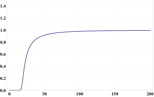
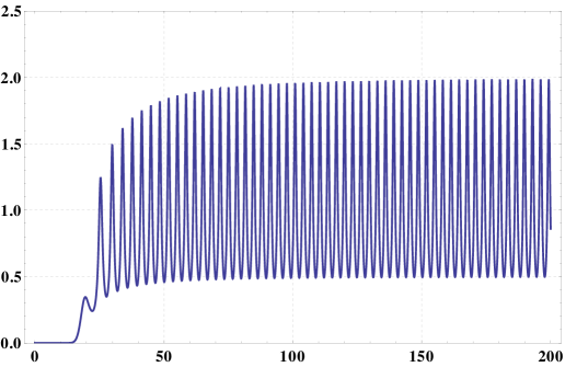
Figure 3: On the left, a plot of the derivative of a phase function associated with the basis of solutions $\{\sqrt{z}J_{20}(z),\sqrt{z}Y_{20}(z)\}$ for (23); on the right, a plot of the derivative of a phase function associated with the basis $\{2\sqrt{z}J_{20}(z),\sqrt{z}Y_{20}(z)\}$. Both are over the interval $[0,200]$.

with $\mu=4\,\nu^{2}$. We note that the asymptotic expansion (43) is only useful because the particular phase function $\alpha_{\nu}(z)$ it represents is non-oscillatory: Figure 3 shows plots of the derivative of the phase function associated with $\{\sqrt{z}J_{\nu}(z),\sqrt{z}Y_{\nu}(z)\}$ and also the derivative of the phase function associated with another choice of basis, $\{2\sqrt{z}J_{\nu}(z),\sqrt{z}Y_{\nu}(z)\}$.

3 Numerical Experiments

In this section we present the result of several numerical experiments conducted to verify the scheme of this paper. The code for these experiments was written in Fortran 77 and compiled using the Intel Fortran compiler version 12.0. Experiments were conducted on a laptop equipped with an Intel Core i7-2620M processor running at 2.70 GHz and 8 GB of RAM. Machine zero was $\varepsilon_{0}=2.22044604925031\times 10^{-16}$.

We constructed asymptotic approximations to the functions $J_{\nu},Y_{\nu}$ via the formulae (33), (35), (43). In order to avoid exceeding the machine exponent, we altered the procedure slightly, so that the coefficients $t_{k},s_{k}$ are never computed by themselves: only the ratios

$${t_{k}\over z^{2k}},\ {s_{k}\over z^{2k}}$$ (45)

are calculated via obvious modifications of (33), (35).

As with all procedures relying on asymptotic expansions, it is not always possible to achieve a desired accuracy. Indeed, the magnitudes of the terms of the expansion reach a certain minimum and then proceed to increase. And, of course, truncating the expansions when the terms become small does not necessarily ensure the accuracy of the approximation (see [9] for numerous examples of possible pathologies). It is shown in Section 13.75 of [13] that if $\nu$ is real, $z$ is positive and $n>\nu-1/2$, then the remainder resulting from the first $n$ terms of expansion (31) is smaller in magnitude than the $(n+1)$st term. However, the authors are not aware of any error bounds for (43) (or for (31) ) in the general case.

Moreover, the value of the phase function $\alpha_{\nu}(z)$ is proportional to the argument $z$ and values of $J_{\nu}(z)$ and $Y_{\nu}(z)$ are obtained in part by evaluating the sine and cosine of $\alpha_{\nu}(z)$. This imposes limitations on the accuracy of the obtained approximations when $z$ is large due to the well-known difficulties in evaluating periodic functions of large arguments.

3.1 Comparison with Mathematica

In these first experiments, we applied the procedure of this paper to the evaluation of the Bessel functions $J_{\nu}(z)$ and $Y_{\nu}(z)$ at various orders and arguments. The resulting values were compared with those produced by version 9.0.0 of Wolfram’s Mathematica package; 30 digit precision was requested from Mathematica. Table 2 reports the results. There, the number of terms used in the expansions of the modulus and phase functions and the relative errors in the obtained values of $J_{\nu}(z)$ and $Y_{\nu}(z)$ are reported.

3.2 Bessel functions of large order.

In this experiment, we approximate the values of Bessel functions of very large orders and arguments. Comparison with other approaches is difficult for such large orders; for instance, Mathematica’s Bessel function routines are prohibitively slow in this regime. We settled for running our procedure twice, once using double precision arithmetic and once using extended precision (Fortran REAL*16) arithmetic in order to produce reference values for comparison.

The first row of each entry in Table 3 reports the relative error in the approximations of $J_{\nu}(z)$ and the second row gives the relative error in the approximation of $Y_{\nu}(z)$. Table 1 gives the number of terms in the expansion of the modulus function and the number of terms in the expansions of the modulus and phase function used to evaluate $J_{\nu}(z)$ and $Y_{\nu}(z)$. These values depended only on the ratio of $z$ to $\nu$ and not on the value of $\nu$.

3.3 Failure for small orders.

In this experiment, we considered the performance of the procedure of this paper for relatively small values of $|\nu|$. We evaluated $J_{\nu}(10\nu)$ at a series of values of $\nu$ between $0$ and $5$. A plot of the base-$10$ logarithm of the relative error in $J_{\nu}(10\nu)$ is shown in Figure 2. Errors were estimated via comparison with Wolfram’s Mathematica package; 30 digit precision was requested from Mathematica.

3.4 Failure as $\mathbf{\mbox{\bf arg}(z)}$ approaches $\mathbf{\pi}$.

In this experiment, we computed the values of $Y_{10}(\exp(i\theta))$ as $\theta$ approaches $\pi$. The obtained values were compared to those reported by Wolfram’s Mathematica package; 30 digit precision was once again requested from Mathematica. A plot of the base-$10$ logarithm of the relative error in $Y_{10}(\exp(i\theta))$ as a function of $\theta$ is shown in Figure 1.

4 Conclusions

We have shown that the Bessel functions $J_{\nu}(z)$ and $Y_{\nu}(z)$ can be efficiently evaluated when $\nu$ is large and $|z|>|\nu|$. This was achieved by representing Bessel functions in terms of a non-oscillatory phase function for which (conveniently enough) a well-known asymptotic expression is available.

The observation underlying the scheme of this paper — namely, the existence of a non-oscillatory phase function — is not a peculiarity of Bessel’s equation. The solutions of a large class of second order linear differential equations can be approximated to high accuracy via non-oscillatory phase functions, a development the authors will report at a later date.

5 Appendix

Here, we formulate a lemma used in Section 2; its proof is an exercise in elementary calculus, and can be found, for example, in [9].

LEMMA 5.1.

Suppose that

$$f(z)\sim 1+\frac{a_{1}}{z^{2}}+\frac{a_{2}}{z^{4}}+\frac{a_{3}}{z^{6}}+\cdots$$ (46)

is an asymptotic expansion for $f:C\to C$, with $a_{1},a_{2},a_{3},\ldots$ a sequence of complex numbers. Then the asymptotic expansion of   $1/f$ is

$$\frac{1}{f(z)}\sim 1+\frac{b_{1}}{z^{2}}+\frac{b_{2}}{z^{4}}+\frac{b_{3}}{z^{6}}+\cdots,$$ (47)

where $b_{1}=-a_{1}$, and the rest of the coefficients $b_{2},b_{3},b_{4},\ldots$ are given by the formula

$$b_{n}=-a_{n}-\sum_{j=1}^{n-1}a_{j}b_{n-j}.$$ (48)

6 Acknowledgments

We would like to thank the reviewer for a careful reading of the manuscript and for several useful suggestions. Zhu Heitman was supported in part by the Office of Naval Research under contracts ONR N00014-10-1-0570 and ONR N00014-11-1-0718. James Bremer was supported in part by a fellowship from the Alfred P. Sloan Foundation and by National Science Foundation grant DMS-1418723. Vladimir Rokhlin was supported in part by Office of Naval Research contracts ONR N00014-10-1-0570 and ONR N00014-11-1-0718, and by the Air Force Office of Scientific Research under contract AFOSR FA9550-09-1-0241.

Figure 1: Failure as $\mathbf{\mbox{\bf arg}(z)}$ approaches $\mathbf{\pi}$. The base-10 logarithm of the relative error in the approximation of $Y_{10}(100\exp(i\theta))$ as $\theta$ approaches $\pi$.

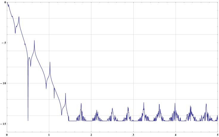
Figure 2: Failure for small orders. The base-10 logarithm of the relative error in the approximation of $J_{\nu}(10\nu)$ plotted as a function of $\nu$.

$z/\nu$	Modulus terms	Phase terms
$1.1$	$162$	$133$
$2$	$024$	$022$
$10$	$008$	$008$
$10\pi$	$006$	$006$

Table 1: Bessel functions of large order. The number of terms in the expansions of the modulus and phase functions used in the computation of Bessel functions of large orders.

		Modulus	Phase	Relative error	Relative error
$\nu$	$z$	terms	terms	in $J_{\nu}(z)$	in $Y_{\nu}(z)$
$50$	$1.1|\nu|$	$049$	$091$	$1.45\times 10^{-14}$	$3.25\times 10^{-14}$
	$2|\nu|$	$023$	$022$	$3.73\times 10^{-14}$	$9.80\times 10^{-15}$
	$10|\nu|$	$008$	$008$	$1.77\times 10^{-14}$	$9.38\times 10^{-15}$
	$100|\nu|$	$005$	$005$	$4.53\times 10^{-13}$	$7.23\times 10^{-14}$
$50-10i$	$1.1|\nu|$	$075$	$098$	$4.85\times 10^{-15}$	$4.81\times 10^{-15}$
	$2|\nu|$	$023$	$022$	$6.04\times 10^{-15}$	$6.12\times 10^{-15}$
	$10|\nu|$	$008$	$008$	$9.79\times 10^{-14}$	$9.77\times 10^{-14}$
	$100|\nu|$	$005$	$005$	$6.31\times 10^{-13}$	$6.31\times 10^{-13}$
$100+20i$	$1.1|\nu|$	$080$	$117$	$1.79\times 10^{-14}$	$1.79\times 10^{-14}$
	$2|\nu|$	$024$	$021$	$3.19\times 10^{-14}$	$3.19\times 10^{-14}$
	$10|\nu|$	$008$	$008$	$1.46\times 10^{-13}$	$1.46\times 10^{-13}$
	$100|\nu|$	$005$	$005$	$5.43\times 10^{-13}$	$5.43\times 10^{-13}$
$10000$	$1.1|\nu|$	$162$	$133$	$1.72\times 10^{-11}$	$4.63\times 10^{-12}$
	$2|\nu|$	$024$	$022$	$1.18\times 10^{-12}$	$6.69\times 10^{-13}$
	$10|\nu|$	$008$	$008$	$8.96\times 10^{-13}$	$1.28\times 10^{-10}$
	$100|\nu|$	$005$	$005$	$1.10\times 10^{-10}$	$2.96\times 10^{-12}$
$100000$	$1.1|\nu|$	$162$	$133$	$5.18\times 10^{-13}$	$7.16\times 10^{-13}$
	$2|\nu|$	$024$	$022$	$4.82\times 10^{-11}$	$2.34\times 10^{-11}$
	$10|\nu|$	$008$	$008$	$1.57\times 10^{-09}$	$3.93\times 10^{-12}$
	$100|\nu|$	$005$	$005$	$1.92\times 10^{-10}$	$2.41\times 10^{-10}$

Table 2: Comparison with Mathematica. The results of the experiments of Section 3.1.

$z$	$\nu=10^{6}$	$\nu=10^{9}$	$\nu=10^{12}$	$\nu=10^{15}$	$\nu=10^{18}$
$1.1\nu$	$1.96\times 10^{-11}$	$4.48\times 10^{-07}$	$3.74\times 10^{-07}$	$3.26\times 10^{-08}$	$5.78\times 10^{-06}$
	$1.18\times 10^{-10}$	$2.81\times 10^{-07}$	$1.70\times 10^{-08}$	$1.57\times 10^{-06}$	$5.87\times 10^{-08}$
$2\nu$	$1.04\times 10^{-10}$	$2.15\times 10^{-07}$	$1.01\times 10^{-07}$	$1.25\times 10^{-07}$	$4.08\times 10^{-07}$
	$4.66\times 10^{-11}$	$6.94\times 10^{-07}$	$1.37\times 10^{-07}$	$2.96\times 10^{-07}$	$7.73\times 10^{-07}$
$10\nu$	$5.25\times 10^{-09}$	$3.80\times 10^{-07}$	$3.20\times 10^{-05}$	$1.09\times 10^{-05}$	$1.04\times 10^{-06}$
	$4.53\times 10^{-10}$	$5.30\times 10^{-07}$	$4.33\times 10^{-09}$	$6.83\times 10^{-08}$	$4.00\times 10^{-06}$
$10\pi\nu$	$3.23\times 10^{-10}$	$4.58\times 10^{-06}$	$7.33\times 10^{-06}$	$3.39\times 10^{-06}$	$4.12\times 10^{-06}$
	$3.80\times 10^{-10}$	$1.01\times 10^{-05}$	$2.10\times 10^{-07}$	$3.68\times 10^{-06}$	$3.05\times 10^{-06}$

Table 3: Bessel functions of large order. The relative errors in the obtained approximations of Bessel functions of large orders: the round-off due to large values of $|z|$ sharply limits the accuracy of results obtainable in double precision

References

- [1] Abramowitz, M., and Stegun, I., Eds. Handbook of Mathematical Functions. Dover, New York, 1964.
- [2] Borůvka, O. Linear Differential Transformations of the Second Order. The English University Press, London, 1971.
- [3] Coddington, E., and Levinson, N. Theory of Ordinary Differential Equations. Krieger Publishing Company, Malabar, Florida, 1984.
- [4] Goldstein, M., and Thaler, R. M. Bessel functions for large arguments. Mathematical Tables and Other Aids to Computation 12 (1958), 18–26.
- [5] Gradstein, I., and Ryzhik, I. Table of Integrals, Sums, Series and Products. Academic Press, 1965.
- [6] Kummer, E. De generali quadam aequatione differentiali tertti ordinis. Progr. Evang. Köngil. Stadtgymnasium Liegnitz (1834).
- [7] Neuman, F. Global Properties of Linear Ordinary Differential Equations. Kluwer Academic Publishers, Dordrecht, The Netherlands, 1991.
- [8] Olver, F. A new method for the evaluation of zeros of bessel functions and of other solutions of second-order differential equations. Proceedings of the Cambridge Philosophical Society 46 (1950), 570–580.
- [9] Olver, F. W. Asymptotics and Special Functions. A.K. Peters, Natick, MA, 1997.
- [10] Spigler, R., and Vianello, M. A numerical method for evaluating the zeros of solutions of second-order linear differential equations. Mathematics of Computation 55 (1990), 591–612.
- [11] Spigler, R., and Vianello, M. The phase function method to solve second-order asymptotically polynomial differential equations. Numerische Mathematik 121 (2012), 565–586.
- [12] Trefethen, N. Approximation Theory and Approximation Practice. Society for Industrial and Applied Mathematics, 2013.
- [13] Watson, G. N. A Treatise on the Theory of Bessel Functions, second ed. Cambridge University Press, New York, 1995.