Facility location problems in the constant work-space read-only memory model

Abstract

Facility location problems are captivating both from theoretical and practical point of view. In this paper, we study some fundamental facility location problems from the space-efficient perspective. Here the input is considered to be given in a read-only memory and only constant amount of work-space is available during the computation. This constant-work-space model is well-motivated for handling big-data as well as for computing in smart portable devices with small amount of extra-space.

First, we propose a strategy to implement prune-and-search in this model. As a warm up, we illustrate this technique for finding the Euclidean 1-center constrained on a line for a set of points in $\mathbb{R}^{2}$. This method works even if the input is given in a sequential access read-only memory. Using this we show how to compute (i) the Euclidean 1-center of a set of points in $\mathbb{R}^{2}$, and (ii) the weighted 1-center and weighted 2-center of a tree network. The running time of all these algorithms are $O(n~{}poly(\log n))$. While the result of (i) gives a positive answer to an open question asked by Asano, Mulzer, Rote and Wang in 2011, the technique used can be applied to other problems which admit solutions by prune-and-search paradigm. For example, we can apply the technique to solve two and three dimensional linear programming in $O(n~{}poly(\log n))$ time in this model. To the best of our knowledge, these are the first sub-quadratic time algorithms for all the above mentioned problems in the constant-work-space model. We also present optimal linear time algorithms for finding the centroid and weighted median of a tree in this model.

1 Introduction

The problem of finding the placement of certain number of facilities so that they can serve all the demands efficiently is a very important area of research. We study some fundamental facility location problems in the memory-constrained environment.

The computational model:

In this paper, we assume that the input is given in a read-only memory where modifying the input during the execution is not permissible. This model is referred as read-only model in the literature and is studied from as early as 80’s [18]. Selection and sorting are well studied in this model [18, 19].

In addition to the read-only model, we assume that only $O(1)$ extra-space each of $O(\log n)$ bits is availabe during the execution. This is widely known as log-space in the computational complexity class [3]. However, we will refer this model as constant-work-space model throughout this paper. This model is well-motivated from the following applications: (i) handling big-data, (ii) computing in a smart portable devices with small amount of extra-space, (iii) in a distributed environment where many procedures access the same data simultaneously.

In this model, as in [6], we assume that a tree $T=(V,E)$ is represented as DCEL (doubly connected edge list) in a read-only memory where for a vertex $u\in V$, we can perform the following queries in constant time using constant space:

• $Parent(u)$: returns the parent of the vertex $u$ in the tree $T$,

• $FirstChild(u)$: returns the first child of $u$ in the tree $T$,

• $NextChild(u,v)$: returns the child of $u$ which is next to $v$ in the adjacency list of $u$.

Here we can perform depth-first traversal starting from any vertex in $O(|V|)$ time.

Definitions and preliminaries:

Let $T=(V,E)$ be a tree where $V$ is the set of vertices (or nodes) and $E$ is the set of edges. The set of points on all the edges of $T$ are also denoted as $T$. Each vertex $u\in V$ has a weight $w(u)$ and each edge $e\in E$ has also a positive length $l(e)$. For any vertex $v\in V$, we denote the degree of $v$ as $d_{v}$. Let $N(v)$ denote the set of adjacent vertices of $v$. The subtrees attached to the node $v$ are denoted as $T_{v^{\prime}}(v)$, where $v^{\prime}\in N(v)$. We denote $T_{v^{\prime}}(v^{+})=T_{v^{\prime}}(v)\cup\{\text{the vertex}~{}v\}\cup\{\text{the edge}~{}(v,v^{\prime})\}$. For any vertex $v\in V$, we denote $MaxS(v)=\max_{v^{\prime}\in{N(v)}}|T_{v^{\prime}}(v)|$, where $|T_{v^{\prime}}(v)|$ denotes the number of vertices in the subtree $T_{v^{\prime}}(v)$. The Centroid of a tree $T=(V,E)$ is a vertex $v^{*}\in V$ such that $MaxS(v^{*})=\min_{v\in V}MaxS(v)$. This can be found in $O(n)$ time using $O(n)$ space [7, 14, 15].

For any point $u\in{T}$, we associate a cost function $SumWD(u)=\sum_{v\in V}d(u,v)w(v)$, where $d(u,v)$ is the distance between $u$ and $v$. The weighted median of ${T}$ is defined as a point $x^{*}$ on the tree ${T}$ such that the associated cost $SumWD(x^{*})$ is minimum over all the points on the edges of the tree $T$. Hakimi [13] showed that there exist a weighted median that lies on a vertex of $T$. So, the weighted median is a vertex $v$ such that $SumWD(v)=\min_{v^{\prime}\in V}SumWD(v^{\prime})$.

For any vertex $v\in{V}$, let $MaxWS(v)=\max_{v^{\prime}\in N(v)}w(T_{v^{\prime}}(v))$, where $w(T_{v^{\prime}}(v))=\sum_{u\in T_{v^{\prime}}(v)}w(u)$. The weighted-centroid of $T$ is defined as a vertex $v^{*}$ with $MaxWS(v^{*})=\min_{v\in V}MaxWS(v)$ [16]. Kariv and Hakimi  [16] showed that a vertex $v$ of a tree ${T}$ is weighted-centroid if and only if $v$ is weighted median. Based on these facts, they present an algorithm to find the weighted median of a tree which runs in $O(n)$ time using $O(n)$ space.

Let $X=\{\alpha_{1},\alpha_{2},\ldots,\alpha_{p}\}$ be a set of $p$ points on the edges of the tree $T$. For any vertex $v\in V$, by $d(X,v)$ we mean $\min_{\alpha\in X}d(\alpha,v)$. The maximum weighted distance from the set $X$ to tree $T$ is denoted by $S(X,T)$, i.e, $S(X,T)=\max_{v\in V}d(X,v)w(v)$. The weighted $p$-center of $T$ is a $p$ sized subset $X$ of $T$ for which $S(X,T)$ is minimum. This problem was originated by Hakimi [13] in 1965 and has a long history in the literature. For any constant p, an $O(n)$ time algorithm using $O(n)$ space is available for this problem[22].

Our main results:

Prune-and-search is an excellent paradigm to solve different optimization problems. First, we propose a framework to implement prune-and-search in the constant-work-space model. As a warm up, we illustrate the technique for finding the Euclidean 1-center constrained on a line for a set of points in $\mathbb{R}^{2}$. This technique works even if the input is given in a sequential access read-only memory. Using this framework we show how to compute (i) the center $c^{*}$ of the minimum enclosing circle for a set of points in $\mathbb{R}^{2}$, and (ii) the weighted 1-center and weighted 2-center of a tree network. The running time of all these algorithms are $O(n~{}poly(\log n))$. The same framework can be applied to other problems which admits solutions by prune-and-search paradigm. For example, we can apply the technique to solve two and three dimensional linear programming in $O(n~{}poly(\log n))$ time in this model. To the best of our knowledge, these are the first sub-quadratic time algorithms for all the above mentioned problems in the constant-work-space model. We also present optimal linear time algorithms for finding the centroid and weighted median of a tree in this model.

Related works:

Constant-work-space model has been studied for a long time and has recently gained more attention. Given an undirected graph testing the existance of a path between any two vertices [21], planarity testing [2], etc. are some of the important problems for which outstanding results on constant-work-space algorithms are available. Selection and sorting are extensively studied in the read-only model [19]. Specially, we want to mention the pioneering work by Munro and Paterson [18], where they proposed $O(n\log^{3}n)$ time constant-work-space algorithm for the selection considering that the input is given in a sequential access read-only memory.

Our work was inspired by an open question from Asano et al. [5] where they presented several constant-work-space algorithms for geometric problems like geodesic shortest path in a simple polygon, Euclidean minimum spanning tree, and they asked for any sub-quadratic time algorithm for minimum enclosing circle in the constant-work-space model. De et al. [12] presented a sub-quadratic time algorithm for the problem using $\Omega(\log n)$ extra-space in the read-only model. An $1.22$ approximation algorithm for minimum enclosing ball for a set of points in $\mathbb{R}^{d}$ using $O(d)$ space is known [1, 10] in the streaming model where only one pass is allowed in the sequential access read-only input. For fixed dimensional linear programming, Chan and Chen [9] presented a randomized algorithm in expected $O(n)$ time using $O(\log n)$ extra-space in the read-only model. We refer [4] for other related recent works in the literature.

2 Prune-and-search using constant work-space

A general scheme for implementing prune-and-search when the input is given in a read-only array is presented in [11, 12] using $\Omega(\log n)$ extra space. Prune-and-search is an iterative algorithmic paradigm. Initially, all the input elements are considered valid and after each iteration a fraction of the valid elements are identified whose deletion will not impact on the optimum result. So, these elements are pruned, and the process is repeated with the reduced set of valid elements until the desired optimum result is obtained or the number of valid elements is a small constant. For the later case, a brute-force search is applied for obtaining the desired result.

In constant-work-space model, after each iteration, we have to distinguish the valid and pruned elements correctly using only $O(1)$ space. Here, we demonstrate that in some special cases, where the combinatorial complexity of the feasible region is $O(1)$ after each iteration, the prune and search can be implemented using $O(1)$ extra space. As a warm up, we describe this using the prune-and-search algorithm for finding the Euclidean 1-center constrained on a line $L$ for a set of points in $\mathbb{R}^{2}$  [17].

2.1 Constrained Euclidean 1-center

A set of $n$ points $P$ in $\mathbb{R}^{2}$ is given in a read-only array $P$ and a vertical line $L$ is given as a query. The objective is to find a point $x^{*}$ on the line $L$ such that the maximum distance of $x^{*}$ from the points of $P$ is minimized over all possible points on $L$.

Megiddo’s Algorithm [17]:

Initially, all the input points are considered as valid. In an iteration, if $n^{\prime}$ is the number of valid elements, then $\frac{n^{\prime}}{2}$ disjoint pairs are formed. Each of these pairs contributes a perpendicular bisector that intersects the line $L$. Considering these $\frac{n^{\prime}}{2}$ intersection points on the line $L$, the algorithm finds the median intersection point $m$ among them. Then it makes the following query:

Query($m$):- decide whether $x^{*}=m$ or $x^{*}$ lies above or below of $m$ on $L$. We compute the farthest point(s) from $m$ among all the valid points. If there exists two farthest points above and below $m$ respectively, then $x^{*}=m$; otherwise, if all the farthest points are in one side, say above (resp. below) of $m$, then $x^{*}$ lies above (resp. below) of $m$ on $L$.

In the former case, the algorithm stops, and in the later case, from each pair whose corresponding perpendicular bisector intersects the line $L$ below (resp. above) $m$, one element is pruned. Thus, in a single iteration, $\frac{n^{\prime}}{4}$ points can be pruned. The next iteration is executed on the remaining valid points unless very few (say, 3 or 4) elements remain as valid, in which case brute-force search is applied to find $x^{*}$.

Figure 1: The input array and the corresponding virtual pairing tree

Overview of our pairing scheme:

We are going to describe a pairing strategy for the prune-and-search algorithm consisting of $O(\log n)$ phase and each phase consists of at most $O(\log n)$ iterations. After each iteration, it will remember a feasible region $U=(a,b)$ on the line $L$ such that the point $x^{*}$ lies in the region $(a,b)$. Initially, $a=-\infty,b=+\infty$, and they are updated after each iteration. This information will help to distinguish the valid and pruned elements. Consider the virtual pairing tree, ${\cal T}$ (See Figure 1), which is a binary tree of depth $d=\lceil\log n\rceil$ and leaves are the input points stored in the read-only array $P$. The subtree rooted at any node $t$ is denoted as $T_{t}$, and the leaves of the tree $T_{t}$ are denoted as $\beta({T_{t}})$. The nodes in the $k$-th ($0<k<d$) level (assuming the leaves are at $1$-st level) represent all the valid points at the beginning of the $k$-th phase of the algorithm. So, the nodes at $k$-th level are actually a subset of valid nodes of $(k-1)$-th level. Any node $t$ at $k$-th level is the only one among $\beta({T_{t}})$ which is valid after $(k-1)$-th phase of the algorithm. The algorithm stops pruning when very few (say, 3 or 4) elements are valid or already $x^{*}$ is found. This virtual pairing tree demonstrates how the pairing is done in each phase of the algorithm.

Let $U=(a,b)$ be the feasible region for the constrained Euclidean 1-center $x^{*}$ on the line $L$. We define a dominance relation as follows.

Definition 1

For a pair of points $p,q\in P$, $p$ is said to dominate $q$ with respect to a feasible region $U$, if their perpendicular bisector $b(p,q)$ does not intersect the feasible region $U$, and both $q$ and $U$ lie on the same side of $b(p,q)$.

It is easy to show from Definition 1 that $p$ dominates $q$ with respect to a feasible region $U$ if and only if from any point $x\in U$, $\widehat{d}(p,x)>\widehat{d}(q,x)$, where $\widehat{d}(p,x)$ (resp. $\widehat{d}(q,x)$) is Euclidean distance between $p$ (resp. $q$) and $x$.

Lemma 1

If $p$ dominates $q$ and $q$ dominates $r$ with respect to a feasible region $U$, then $p$ dominates $r$ with respect to the feasible region $U$.

Proof:   Let $x$ be an arbitrary point in $U$. Since $p$ dominates $q$, $\widehat{d}(p,x)>\widehat{d}(q,x)$. Since $q$ dominates $r$, $\widehat{d}(q,x)>\widehat{d}(r,x)$. Thus $\widehat{d}(p,x)>\widehat{d}(r,x)$.  $\Box$

First phase

The feasible region $U=(a,b)$ is initialized as $(-\infty,\infty)$. Now, all the points in $P$ are valid. We form pairs, $Pair_{i}^{1}=(P[2i-1],P[2i])$, $i=1,2,\ldots,\lfloor\frac{n}{2}\rfloor$. A pair $Pair_{i}^{1}$, $i\in\{1,2\ldots,\lfloor\frac{n}{2}\rfloor\}$ is considered to be a valid pair with respect to $(a,b)$ if the corresponding perpendicular bisector intersects $(a,b)$ on the line $L$.

In an iteration, we consider only the valid pairs with respect to $(a,b)$ (in the first iteration, all the pairs are valid). Considering the intersection points of the perpendicular bisectors of these valid pairs with $L$, we compute the median intersection point $m$ on $L$. Then we perform Query($m$) by inspecting all the points of $P$ as in Megiddo’s algorithm. Depending on the answer of the query, either $x^{*}$ is found, or $U$ is updated by assigning $a$ or $b$ with $m$. In the former case, the algorithm stops and in the later case, from each of the pairs whose corresponding perpendicular bisector intersects $L$ outside the revised $(a,b)$, one element is pruned. So, after this iteration, one element each from at least $\frac{1}{4}$-th of the valid pairs is pruned. The algorithm executes next iteration with the remaining valid pairs. The process continues until from each pair $Pair_{i}^{1}$, $i=1,2,\ldots,\lfloor\frac{n}{2}\rfloor$, one element is pruned. Since, after each iteration, one element from at least $\frac{1}{4}$-th of the valid pairs is pruned, this phase executes at most $O(\log n)$ iterations. Finally, after completion of this phase, we can discard $\lfloor\frac{n}{2}\rfloor$ points, i.e, one point from each of the pair $Pair_{i}^{1}$, $i=1,2,\ldots,\lfloor\frac{n}{2}\rfloor$.

$k$-th phase

At the beginning of the $k$-th phase, let $U=(a,b)$ and we know that only one element is valid (i.e. dominant) from each block of consecutive $2^{k-1}$ elements, namely $B_{i}^{k}=\{P[i.2^{k-1}+1],P[i.2^{k-1}+2],\ldots,P[(i+1).2^{k-1}]\}$, $i=1,2,\ldots,\lfloor\frac{n}{2^{k-1}}\rfloor$. For the last block $B_{\lceil\frac{n}{2^{k-1}}\rceil}^{k}$, the members are $\{P[i.2^{k-1}+1],P[i.2^{k-1}+2],\ldots P[n]\}$. We denote the only valid element of a block $B_{i}^{k}$ as $valid(B_{i}^{k})$. Now, the most important task is to recognize the $valid(B_{i}^{k})$ for all $i=1,2,\ldots,\lceil\frac{n}{2^{k-1}}\rceil$. In this regard, we have the following:

Lemma 2

The $valid(B_{i}^{k})$ can be identified in $O(|B_{i}^{k}|)$ time using $O(1)$ extra-space, where $i=1,2,\ldots,\lceil\frac{n}{2^{k-1}}\rceil$ and $0<k<d$.

Proof:   The transitivity of the dominance relation (see Lemma 1) and the pairing strategy guarantee that $valid(B_{i}^{k})$ dominates all other elements of the block $B_{i}^{k}$. For the block $B_{i}^{k}$, we initialize two variables $candidate=i.2^{k-1}+1$ and $pointer=i.2^{k-1}+2$.

In the first step, we pair up $(P[candidate],P[pointer])$ and observe their perpendicular bisector. Here either of the two situation occurs. (i) If the perpendicular bisector of the pair intersects the feasible region $U$, then none of these two points is $valid(B_{i}^{k})$. We update $candidate=pointer+1$ and $pointer=pointer+2$. (ii) Otherwise, one of the points of $(P[candidate],P[pointer])$ dominates the other. We update the variable $candidate$ with the index of the dominating one and $pointer=pointer+1$.

We repeat the next step with new pair until the variable $pointer$ reaches the last element of the block $B_{i}^{k}$. At the end, we obtain $valid(B_{i}^{k})=P[candidate]$. Thus, the lemma follows.  $\Box$ Thus, in this phase, we can correctly enumerate all the valid elements in $O(n)$ time using $O(1)$ space.

As in the first phase, we construct pairs $Pair_{i}^{k}=(valid(B_{2i-1}^{k}),valid(B_{2i}^{k}))$, for $i=1,2,\ldots,\lceil\frac{n}{2^{k-1}}\rceil$, and consider a pair $Pair_{i}^{k}$ to be a valid pair with respect to $(a,b)$ if the corresponding perpendicular bisector intersects $(a,b)$ on $L$. Here also we need at most $O(\log(\lceil\frac{n}{2^{k-1}}\rceil))$ iterations to discard one element from each $Pair_{i}^{k}$. Needless to say, during this process $x^{*}$ may also be found. Thus, after this phase from each of the block $B_{i}^{k+1}$, $i=0,1,\ldots\lceil\frac{n}{2^{k}}\rceil$, only one element survives.

As the depth of the virtual pairing tree is $O(\log n)$, so there are at most $O(\log n)$ phases. Each phase needs at most $O(\log n)$ iterations, each of which needs $O(n+M)$ time. Here $M$ is the time needed to compute the median of $n$ elements in the read-only memory when $O(1)$ space is provided [18, 19, 20]. Thus we have the following theorem.

Theorem 1

Given a set of $n$ points in $\mathbb{R}^{2}$ in a read-only memory and a line $L$, the Euclidean 1-center constrained on a line $L$ can be found in $O((n+M)\log^{2}n)$ time using $O(1)$ extra-space, where $M$ is the time needed to compute the median of $n$ elements given in a read-only memory using $O(1)$ extra-space.

Remark 1

Note that our pairing strategy will work even if the input is given in sequential access read-only memory. Here the median finding algorithm is appropriately chosen for the sequential access read-only memory [18]. For detailed literature on selection, we refer [8].

3 Euclidean 1-Center

Problem Statement

The Euclidean 1-center of a set $P$ of $n$ points in $\mathbb{R}^{2}$ is a point $c^{*}\in\mathbb{R}^{2}$ for which the maximum distance from any point in $P$ is minimized. The point $c^{*}$ is actually the center of the minimum enclosing circle of $P$. Here, we assume that the input is given in a read-only memory and only constant amount of work-space is available for the computation.

Megiddo’s Algorithm [17]:

This is a prune-and-search algorithm that uses the following sub-routine. Decide-on-a-Line($L$): Given a set of points $P$ in $\mathbb{R}^{2}$ and a query line $L$, decide in which side of $L$ the Euclidean 1-center $c^{*}$ for the points in $P$ lies.

In Megiddo’s algorithm, initially all the input points are considered to be valid. In an iteration, if $n^{\prime}$ is the number of valid points, then $\lfloor\frac{n^{\prime}}{2}\rfloor$ disjoint pairs are formed. Each pair contributes a perpendicular bisector. Let us denote this set of perpendicular bisectors as ${\cal P_{B}}$. Compute the median slope $S_{m}$ of these bisectors. A perpendicular bisector $b_{i}\in{\cal P_{B}}$ with slope less than $S_{m}$ is paired with a perpendicular bisector $b_{i}\in{\cal P_{B}}$ having slope greater than or equal to $S_{m}$. In this way, $\lfloor\frac{n^{\prime}}{4}\rfloor$ disjoint pairs of bisectors are formed. Each pair of bisectors contribute an intersection points. So there are $\lfloor\frac{n^{\prime}}{4}\rfloor$ intersection points. Let us denote this set of intersection points as $I$. The intersection point $t\in I$ with median $x$-coordinate (with respect to rotated coordinate system by an angle $S_{m}$) is identified. Now, the subroutine Decide-on-a-Line is evoked for the line $L_{1}$ passing through $t$ with slope $S_{m}$ to decide in which side of $L_{1}$ the point $c^{*}$ lies. Next, consider the intersection points of $I$ which lies to the side of $L$ opposite to $c^{*}$, and find the intersection point $t^{\prime}$ having median $y$-coordinate value (with respect to rotated coordinate system by an angle $S_{m}$). Let $L_{2}$ be the line perpendicular to $L_{1}$ and passing through $t^{\prime}$. We evoke the subroutine Decide-on-a-Line for the line $L_{2}$. Thus, a quadrant $Q$ is defined by the two lines $L_{1}$ and $L_{2}$ which contains $c^{*}$. The choice of the lines $L_{1}$ and $L_{2}$ guarantees that $\frac{n^{\prime}}{16}$ perpendicular bisectors from ${\cal P_{B}}$ will not intersect the quadrant $Q$. This allows us to prune a point corresponding to each of those perpendicular bisectors. As a result, after each iteration at least $\frac{n^{\prime}}{16}$ of the valid points are pruned. The iteration is repeated for the rest of the valid points until the number of valid points become very small (say 15), or already $c^{*}$ is found. In the former case, brute-force is applied to compute the point $c^{*}$.

Our implementation of the algorithm in constant work-space model:

First, we show that Decide-on-a-Line($L$) can be answered using $O(1)$ extra-space.

Lemma 3

For a set of $n$ points $P$ in $\mathbb{R}^{2}$, Decide-on-a-Line($L$) can be computed in $O((n+M)\log^{2}n)$ time using $O(1)$ extra-space, where $M$ is the time needed to compute the median of $n$ elements given in a read-only memory using $O(1)$ extra-space.

Proof:   By Theorem 1, we can compute the constrained Euclidean 1-center $x^{*}$ on the line $L$ in $O((n+M)\log^{2}n)$ time using $O(1)$ extra-space. Now, in a single scan over all the points in $P$, we can identify the farthest point(s) from $x^{*}$. Let $F$ be the set of points that are farthest from $x^{*}$.

Step 1:

By scanning the whole array, we can decide whether all the points in $F$ are in one side of $L$. If the test is positive, then $c^{*}$ will be in the same side of $L$; otherwise we go to the next step.

Step 2:

Now, the points of $F$ are in both side of the line $L$. If the convex hull defined by $F$ contains $x^{*}$, then $c^{*}=x^{*}$. For this, we do not have to construct the convex hull explicitly. Let $t_{1}$ and $b_{1}$ (resp. $t_{2}$ and $b_{2}$) be the two points of $F$ in one side of $L$ whose projections on $L$ are the farthest apart. Consider two lines joining $t_{1},t_{2}$ and $b_{1},b_{2}$ and observe their intersections with the line $L$. The convex hull of $F$ contains $x^{*}$ if and only if $x^{*}$ is in between these two intersection points because the points in $F$ are in a circle whose center is $x^{*}$. In the positive case, $c^{*}=x^{*}$. Otherwise, we go to the next step.

Step 3:

Now, the midpoint of the line joining the farthest pair of points in $F$ will determine the side of $L$ in which $c^{*}$ lies. In this case either $(t_{1},t_{2})$ or $(b_{1},b_{2})$ are the farthest pair of points in $F$.

Thus the lemma follows.  $\Box$

We implement Megiddo’s algorithm in a similar way as described in Section 2.1. Note that in our scheme, we need to remember a feasible region $U$ for $c^{*}$ of constant combinatorial complexity after each iteration. Here, after each iteration, we get a quadrant (defined by a pair of mutually perpendicular lines $L_{1}$ and $L_{2}$) that contains the $c^{*}$. But considering all the iterations, the intersection of all these quadrants has combinatorial complexity $O(\log n)$. So, the straight-forward implementation will not lead to an algorithm in constant-work-space model. To overcome this, we apply the following simple trick. After each iteration we will remember a feasible region $U$ as a triangle. After the first iteration of the algorithm we have a quadrant $Q$ in which $c^{*}$ lies. We obtain a triangle $T\subset Q$ containing $c^{*}$ using the following lemmas.

Lemma 4

If we know a quadrant $Q$ in which $c^{*}$ lies, then we can obtain a triangle $T\subseteq Q$ containing $c^{*}$ by evoking the subroutine Decide-on-a-Line($L$) once more.

Proof:   We scan the points in $P$ to find the axis-parallel rectangle $R$ containing all the points in $P$. Observe that $R$ contains $c^{*}$. The polygon $R^{\prime}=R\cap Q$ has at most four side. If $R^{\prime}$ is a triangle, then $T=R^{\prime}$. Otherwise, by evoking the subroutine Decide-on-a-Line($L$) on any diagonal of the quadrangle $R^{\prime}$, we can decide a triangle $T\subset R^{\prime}$ containing $c^{*}$.  $\Box$

Lemma 5

Let $T$ be a triangle and $Q$ be a quadrant both of which contain the Euclidean 1-center $c^{*}$. We can obtain another triangle $T^{\prime}\subseteq T\cap Q$ containing $c^{*}$ by evoking the subroutine Decide-on-a-Line($L$) at most twice.

Proof:   Note that the $R=T\cap Q$ is a polygon with at most five sides. So, we can triangulate the polygon $R$ using at most two diagonals. By evoking Decide-on-a-Line($L$) on each of these diagonals, we can decide the triangle $T^{\prime}$ containing $c^{*}$.  $\Box$

Observe that any perpendicular bisector which does not intersect $Q$ and $T$ also does not intersect $T^{\prime}$. Thus, we remember a triangular feasible region $U$ for $c^{*}$ using $O(1)$ extra-space. Now, we apply our constant-work-space pairing strategy to this modified algorithm. Here, again we have $O(\log n)$ phase each consisting of $O(\log n)$ iterations. In the beginning of the $k$-th phase, we know only one element is valid from each block $B_{i}^{k}$ of consecutive $2^{k-1}$ elements. Similar to Definition 1, here also we can define dominance relation with respect to the feasible region $U$ and it is easy to prove that Lemma 1 and 2 hold. We construct pairs $Pair_{i}^{k}=(valid(B_{2i-1}^{k}),valid(B_{2i}^{k}))$, for $i=1,2,\ldots,\lceil\frac{n}{2^{k-1}}\rceil$. A pair $Pair_{i}^{k}$ is considered a valid pair with respect to the feasible region $U$, if the perpendicular bisector of that pair intersects $U$. In an iteration, by making at most four calls to the subroutine Decide-on-a-Line($L$), we update our feasible region $U$ which guarantees that one point each from at least $\frac{1}{16}$-fraction of the valid pairs are pruned with respect to $U$. As each iteration takes $O((n+M)\log^{2}n)$ time and $O(1)$ extra-space (by Lemma 3, 4 and 5) and there are at most $O(\log^{2}n)$ iterations, the running time of this algorithm is $O((n+M)\log^{4}n)$, where $M$ is the time required to compute the median of a set of $n$ elements in the constant work-space model. Thus we have the following result.

Theorem 2

Given a set of $n$ points in $\mathbb{R}^{2}$, we can compute the Euclidean 1-center in $O((n+M)\log^{4}n)$ in the constant-work-space model, where $M$ is the time required to compute the median of $n$ elements in the constant work-space model.

4 Centroid of a tree

The quadratic time algorithm for finding the centroid of a tree $T=(V,E)$ in the constant-work-space model is quite obvious. For each vertex $v\in V$, compute $MaxS(v)=\max_{v^{\prime}\in N(v)}|T_{v^{\prime}}(v)|$ by inspecting all its neighbors’ subtree, and finally report the centroid of $T$ which is a vertex with minimum $MaxS(v)$ value.

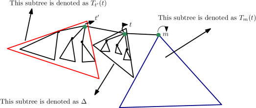
Figure 2: Illustration for the definitions

In this section, we present a linear time algorithm for finding the centroid of a tree $T$ using only constant amount of extra-space. This algorithm is similar to the $O(n)$ time and $O(n)$ space algorithm given in [15] for the same problem. Here $n=|V|$. It is based on the fact that a vertex $v^{*}\in V$ is the centroid if and only if $MaxS(v^{*})\leq\lfloor\frac{n}{2}\rfloor$ (see [14]).

Our algorithm starts from an arbitrary vertex $t$ (say the $t=root(T)$) and finds it’s adjacent vertex $m$ such that $|T_{m}(t)|=MaxS(t)=\max_{v^{\prime}\in N(v)}|T_{v^{\prime}}(t)|$. If $|T_{m}(t)|\leq\lfloor\frac{n}{2}\rfloor$, then $t$ is the centroid; otherwise $t$ can not be the centroid and the centroid must be in the subtree $T_{m}(t)$. In the later case, we will continue to search in the subtree $T_{m}(t)$ ignoring $T\setminus T_{m}(t)$. The pseudo-code of our algorithm is given in Algorithm 1. Here, we use the variables $t$, $t^{\prime}$ and $Size$, maintaining the following invariant.

Invariant 1

• Initially, $t=root(T)$, $t^{\prime}=\emptyset$ and $Size=0$.

• If $t^{\prime}\neq\emptyset$, then $t$ and $t^{\prime}$ are adjacent vertices of $T$ and $Size=|T_{t^{\prime}}(t)|$

Input: A tree $T$ is given in a read-only memory

Output: Report the centroid of the given tree

1 $t=root(T)$; $t^{\prime}=\emptyset$; $Size=0$;

2

3do

4       $(m,\delta,TMsize)=\textsf{\sc Find-Maximum-Subtree}(t,t^{\prime},Size)$;

5       if $TMsize>\lfloor\frac{n}{2}\rfloor$ then

6            $t^{\prime}=t$; $t=m$; $Size=Size+\delta$ ;

7      

8while $TMsize\leq\lfloor\frac{n}{2}\rfloor$;

9Return $t$;

Algorithm 1 Centroid($T$)

At each iteration of the do-while loop, the algorithm evokes the procedure Find-Maximum-Subtree($t,t^{\prime},Size$) which returns three parameters $m$, $\delta$ and $TMsize$. Here $m$ is the adjacent vertex of $t$ such that $|T_{m}(t)|=MaxS(t)=\max_{v^{\prime}\in N(v)}|T_{v^{\prime}}(t)|$. Here $TMsize=|T_{m}(t)|$ and $\delta$ is the number of vertices in the subtree $\Delta=T\setminus\{T_{t^{\prime}}(t)\cup T_{m}(t)\}$ (see Figure 2). Now, depending on the value of $TMsize$, following two cases arise.

• If $TMsize\leq\lfloor\frac{n}{2}\rfloor$, then $t$ is the centroid. In this case, the algorithm stops execution after reporting $t$.

• Otherwise (i.e $TMsize>\lfloor\frac{n}{2}\rfloor$), $t$ is not the centroid. Here $t^{\prime}$ is updated to $t$; $t$ is updated to $m$ and $Size$ is incremented by $\delta$. Then it repeats the iteration of the do-while loop.

Note that, as $TMsize+Size=|T_{m}(t)|+|T_{t^{\prime}}(t)|$ and the value of $Size$ monotonically increases after each iteration, the loop will definitely terminate. The correctness of the algorithm follows from the fact that a centroid can not have a subtree of size greater than $\lfloor\frac{n}{2}\rfloor$ [14].

Lemma 6

The procedure Find-Maximum-Subtree($t,t^{\prime},Size$), which returns three parameters $m$, $\delta$ and $TMsize$, can be implemented in $O(2\delta)$ time using $O(1)$ extra-space. Here $m$ is vertex adjacent to $t$ such that $|T_{m}(t)|=\max_{v^{\prime}\in N(v}|T_{v^{\prime}}(t)|$, $TMsize=|T_{m}(t)|$ and $\delta$ is the number of vertices in the subtree $\Delta$, where $\Delta=T\setminus\{T_{t^{\prime}}(t)\cup T_{m}(t)\}$ (see Figure 2).

Proof:   We implement the procedure Find-Maximum-Subtree($t,t^{\prime},Size$) by a similar way as Asano et al. [6] did for their FindFeasibleSubtree. Note that using the three routines, namely $Parent(v^{\prime})$, $FirstChild(v^{\prime})$, $NextChild(t,v^{\prime})$, we can compute the number of vertices in the subtree $T_{v^{\prime}}(t)$ by a depth-first traversal for any vertex $v^{\prime}\in V$ . It takes $O(|T_{v^{\prime}}(t)|)$ time and $O(1)$ extra-space.

We maintain a pointer variable $m$ and two integer variables $TMsize$ and $ENC$. They are initialized as $m=t^{\prime}$, $TMsize=Size$ and $ENC=0$, respectively. At any moment during the execution of the procedure, $m$, $TMsize$ and $ENC$ signify, so far obtained, the subtree with maximum size, the size of the maximum sized subtree and the number of vertices traversed, respectively.

As $Size$ signifies $|T_{t^{\prime}}(t)|$ (by Invariant 1), we already know the size of the subtree $T_{t^{\prime}}(t)$. So, we do not need to perform a depth-first-traversal in the subtree $T_{t^{\prime}}(t)$. We start computing the number of vertices for two subtrees in parallel using two pointers $\pi_{1}$ and $\pi_{2}$ (in sequential machine one move of $\pi_{1}$ is followed by one move in $\pi_{2}$, and vice versa). While traversing a subtree by $\pi_{i}$, its root is stored in $\phi_{i}$, $i=1,2$. For each $\pi_{i}$, a variable $\chi_{i}$ is maintained that stores the number of vertices encountered by $\pi_{i}$. If one of $\pi_{1}$ and $\pi_{2}$ completes its task in a subtree, then it start traversal in the next unprocessed subtree. After each step, $ENC$, $\chi_{1},\chi_{2}$ are updated. The variables $m$ and $TMsize$ are updated accordingly. The process terminates when one of $\pi_{i}$ (say $\pi_{1}$) finds that there is no more subtree to process. Thus the remaining subtree $T_{\phi_{2}}(t)$ of the other pointer ($\pi_{2}$) is not traversed completely, but we can compute the number of vertices in that subtree as $n-Size-ENC+\chi_{2}$, and update $m$ and $TMsize$, if needed. We compute the number of vertices in the subtree $\Delta$ as $\delta=(n-Size-TMsize)$.

Thus, when the process stops, both $\pi_{1}$ and $\pi_{2}$ traversed equal number of elements. As all the subtrees in $\Delta$ can be processed in at most $2\delta$ steps, so the time needed for the procedure Find-Maximum-Subtree($t,t^{\prime}$) is at most $2\delta$, where $\delta$ is the number of vertices in $\Delta$. From the description, it is obvious that we need only $O(1)$ extra-space.  $\Box$

Time complexity analysis

The complexity of each do-while loop is the time needed for the procedure Find-Maximum-Subtree which is at most $2\delta$ (see Lemma 6). As the value of the variable $Size$ is incremented by $\delta$ after each iteration of the do-while loop, the time complexity of our algorithm is $O(2\times Size)$, where $Size$ is the final value of $Size$ after the completion of the do-while loop. As the maximum value of $Size$ (i.e $|T_{t^{\prime}}(t)|$) is bounded by $n$, so the time complexity of the algorithm is $O(n)$. Thus, we have the following:

Theorem 3

The centroid of a tree, given in a read-only memory, can be computed in $O(n)$ time using $O(1)$ extra-space.

5 Weighted 1-center of a tree

Our approach to compute the weighted 1-center of a tree in constant-work-space model is similar to the $O(n\log n)$ time $O(n)$ extra-space algorithm proposed by Kariv and Hakimi [15]. Overview of the algorithm is as follows. First, it finds an edge $e^{*}$ where the center of the weighted 1-center lies. Next, it finds the absolute weighted 1-center on that edge $e^{*}$ using prune-and-search.

5.1 Finding the edge $e^{*}$

Kariv and Hakimi’s [15] prune-and-search based algorithm for finding the edge $e^{*}$ is based on the following:

Lemma 7

If $c$ is a fixed vertex of the tree $T=(V,E)$ and $v^{\prime}$ is a vertex in the subtree $T_{t}(c)$ ($t\in N(c)$) satisfying $w(v^{\prime})d(v^{\prime},c)=\max_{v\in V}w(v)d(v,c)$, then the 1-center of $T$ is in the subtree $T_{t}(c^{+})$.

It initializes $T^{\prime}=T$. In each iteration, it finds the centroid $c$ of $T^{\prime}$, and identifies a vertex $v^{\prime}$ satisfying Lemma 7 by traversing all the vertices of $T$. Thus the subtree ${T}^{\prime}_{t}(c)$, containing $v^{\prime}$, is identified. Then, it sets $T^{\prime}=T^{\prime}\cap{T}^{\prime}_{t}(c^{+})$, and unless $T^{\prime}$ is an edge it repeats the next iteration. Since $c$ is the centroid, in each iteration a subtree containing at least $\frac{|T^{\prime}|}{2}$ vertices is pruned. Thus, the number of iterations is $O(\log n)$ in the worst case. Though the time complexity of computing the centroid is $O(|T^{\prime}|)$ [15], the time taken for identifying the subtree of $c$ containing $v^{\prime}$ is $O(|T|)$ as it needs to traverse all the vertices of $T$. Thus, the overall time complexity of this algorithm is $O(n\log n)$.

In Section 4, we have already shown that centroid of a tree $T^{\prime}$ can be computed in $O(|T^{\prime}|)$ time in the constant-work-space model. In order to make this algorithm work in constant-work-space model, we have to make sure that $T^{\prime}$ can be identified from $T$ using $O(1)$ extra-space.

(a)

(b)

Figure 3: $T^{\prime}$ is the red portion of the tree

Observe that after each iteration at most two internal nodes of $T$ may become leaves of $T^{\prime}$. So $T^{\prime}$ may have $O(\log n)$ leaves which are internal vertices of the original tree $T$ (see Figure 3(a) where red portion indicates $T^{\prime}$). Such a representation of $T^{\prime}$ can not be encoded using $O(1)$ extra-space. To overcome this, we modify the algorithm maintaining the following invariant:

Invariant 2

At most two internal vertices of $T$ are leaves of $T^{\prime}$.

This invariant enables us to encode $T^{\prime}$ using only four variables $u_{1},v_{1},u_{2}$ and $v_{2}$ as follows.

• If $(u_{i},v_{i})\neq(\emptyset,\emptyset)$ for both $i=1$ and $2$ (i.e $T^{\prime}$ has two internal nodes of $T$ as leaves), then $T^{\prime}=T_{v_{1}}(u_{1}^{+})\cap T_{v_{2}}(u_{2}^{+})$ ((see Figure 3(b));

• Else if $(u_{i},v_{i})\neq(\emptyset,\emptyset)$ for $i=1$ or $i=2$ (i.e $T^{\prime}$ has one internal node of $T$ as leaf), then $T^{\prime}=T_{v_{i}}(u_{i}^{+})$;

• Else $T^{\prime}=T$.

We use another variable $root^{\prime}$ which signifies the root of the tree $T^{\prime}$. If any one of $(u_{i},v_{i})\neq(\emptyset,\emptyset)$ and $(u_{i})$ is the parent of $v_{i}$, then $root^{\prime}=u_{i}$; otherwise, $root^{\prime}=root(T)$.

The pseudo-code of our algorithm is given in Appendix-2 as Algorithm 3. In each iteration, we compute the centroid $c$ of $T^{\prime}$ as stated in Section 4. Next, by traversing the whole tree $T$, we find the subtree $T_{t}(c^{+})$ which contain a vertex $v^{\prime}$ satisfying Lemma 7. Here one of the following two situations arises. (i) If at most one of $u_{i}$ $i\in\{1,2\}$ is in the subtree $T_{t}(c^{+})$, then $T^{\prime}\cap T_{t}(c^{+})$ has at most two internal nodes of $T$ as leaves. (ii) Otherwise, if both $u_{1}$ and $u_{2}$ are in the subtree $T_{t}(c^{+})$, then $T^{\prime}\cap T_{t}(c^{+})$ may have at most three internal nodes of $T$ (namely $c$ , $u_{1}$ and $u_{2}$) as leaves. We can test this in $O(n)$ time using $O(1)$ extra-space. In the former case, we set $T^{\prime}=T^{\prime}\cap T_{t}(c^{+})$ by updating $(u_{i},v_{i})$ for the desired $i\in\{1,2\}$. In the later case, if three internal vertices appear in $T^{\prime}\cap T_{t}(c^{+})$, we do the following.

• First, we compute the junction($c,u_{1},u_{2}$) which is a vertex $j$ of the subtree $T^{\prime}\cap T_{t}(c^{+})$ such that $c$, $u_{1}$ and $u_{2}$ are in three different subtrees $T_{k_{\ell}}(j)$, $k_{\ell}\in N(j)$ for $\ell=1,2,3$. It is left to the reader to verify that one can compute the junction($c,u_{1},u_{2}$) in $O(n)$ time using $O(1)$ extra-space.

• Next, we compute $S(j,T)=\max_{v\in V}w(v)d(v,j)$ and find an adjacent vertex of $j$ such that the subtree ${T}_{t^{\prime}}(j)$ contains a vertex $v^{\prime\prime}$ for which $w(v^{\prime\prime})d(v^{\prime\prime},j)=\max_{v\in V}w(v)d(v,j)$ (satisfying Lemma 7). Note that, as $j$ is the junction($c,u_{1},u_{2}$), ${T}_{t^{\prime}}(j)$ can contain at most one of $u_{1}$, $u_{2}$ and $c$. As a result, $T^{\prime}\cap T_{t}(c^{+})\cap{T}_{t^{\prime}}(j)$ has at most two internal nodes of $T$ as leaves. So, we appropriately update $T^{\prime}=T^{\prime}\cap T_{t}(c^{+})\cap{T}_{t^{\prime}}(j)$ by updating $(u_{i},v_{i})$ for $i=1,2$.

Using induction, we can prove that the Invariant 2 is maintained after each iteration. This is to be observed that $T^{\prime}$ is decreased by at least half after each iteration. Thus, we have the following result.

Lemma 8

For a tree $T$ given in a read-only-memory, one can obtain the edge $e^{*}$ where the center of the weighted 1-center lies in $O(n\log n)$ time using $O(1)$ extra-space.

5.2 Computing weighted 1-center on the edge $e^{*}$

We find the weighted 1-center $c^{*}$ on the edge $e^{*}=(u^{*},v^{*})$ using prune-and-search algorithm similar to Section 2.1. Let $V_{1}$ and $V_{2}$ be the set of vertices in the tree $T_{u^{*}}(v^{*})$ and $T_{v^{*}}(u^{*})$, respectively. Each vertex $v\in V_{1}$ (resp. $v\in V_{2}$) contributes a linear function $f_{1}(v,x)=w(v)d(u^{*},v)+w(v)d(x,u^{*})$ (resp. $f_{2}(v,x)=w(v)d(v^{*},v)+w(v)d(x,v^{*})$) which signifies the weighted distance from $v$ to a point $x\in e^{*}$. In this regard, it is easy to prove the following:

Lemma 9

All the vertices $v\in V_{1}$ (resp. $v\in V_{2}$) and the corresponding distance $d(u^{*},v)$ (resp. $d(v^{*},v)$) can be enumerated in some order in $O(n)$ time using $O(1)$ extra-space.

As in Section 2.1, given a point $m\in(a,b)$ here also we use Query($m$) to decide whether $m$ is the $c^{*}$ or $c^{*}$ lies in $(a,m)$ or in $(m,b)$. For each vertex $v\in V_{1}$ (resp. $v\in V_{2}$), we compute the $f_{1}(v,m)$ (resp. $f_{2}(v,m)$) and find the one with maximum $f_{1}(v,m)$ (resp. $f_{2}(v,m)$) value. Let $k_{1}\in V_{1}$ and $k_{2}\in V_{2}$ be two vertices for which the $f_{1}(k_{1},m)$ and $f_{2}(k_{2},m)$ are maximum, respectively. If $f_{1}(k_{1},m)=f_{2}(k_{2},m)$, then $m$ is the $c^{*}$; else if $f_{1}(k_{1},m)>f_{2}(k_{2},m)$, then $c^{*}\in(a,m)$, otherwise $c^{*}\in(m,b)$. So, we can answer Query($m$) in $O(n)$ time using $O(1)$ space.

Here we define the dominance relation as follows:

Definition 2

For a pair of vertices $p,q\in V_{1}$ (resp. $p,q\in V_{2}$ ), $p$ is said to dominate $q$ with respect to a feasible region $U=(a,b)$, if their corresponding functions $f_{1}(p,x)$ and $f_{1}(q,x)$ (resp. $f_{2}(p,x)$ and $f_{2}(q,x)$ ) does not intersect within the feasible region $U=(a,b)$ and the value of $f_{1}(q,x)<f_{1}(p,x)$ (resp. $f_{2}(q,x)<f_{2}(p,x)$ ) for $x\in U=(a,b)$.

Note that if $f_{1}(p,x)$ and $f_{1}(q,x)$ do not intersect within the feasible region $U=(a,b)$, then by checking at any point $x\in U=(a,b)$, we can decide which one is dominating. It is left to the reader to verify that this relation also satisfies the following lemma.

Lemma 10

If $p$ dominates $q$ and $q$ dominates $r$ with respect to a feasible region $U=(a,b)$, then $p$ dominates $r$ with respect to the feasible region $U=(a,b)$.

Now, we follow the pairing strategy as given in Section 2.1. Initially, we consider that all the vertices in $V_{1}$ (resp. $V_{2}$) are valid and the feasible region for $c^{*}$ is $U=(a,b)=(u^{*},v^{*})$. At the beginning of each phase, we pair up the consecutive valid elements of $V_{1}$ (resp. $V_{2}$) in a similar fashion as described in Section 2.1. A pair of vertices $(v_{1},v_{2})$ contributes an intersection point $i(v_{1},v_{2})=\frac{w(v_{1})d(u^{*},v_{1})-w(v_{2})d(u^{*},v_{2})}{w(v_{2})-w(v_{1})}$ of their corresponding function $f_{1}$ (resp. $f_{2}$). A constructed pair $(v_{1},v_{2})$ is considered as a valid pair with respect to $U$ if the corresponding intersection point $i(v_{1},v_{2})$ lies in $U$, otherwise we can prune one of $v_{1}$ and $v_{2}$ depending on whose $f_{1}$ (resp. $f_{2}$) value is less in $(U)$. We find the median $m$ of these intersection values considering all the valid pairs and perform Query($m$). So, after this we can prune one element each from at least $\frac{1}{4}$-th of the valid pairs. After at most $O(\log n)$ iterations, we can prune one element from each of the valid pairs. Following the same frame-work as given in Section 2.1, we have the following:

Theorem 4

The weighted 1-center of a tree $T$ can be computed in $O((n+M)\log^{2}n)$ time using $O(1)$ extra-space in the constant-work-space model, where $M$ is the time needed to compute the median of $n$ elements given in a read-only memory when $O(1)$ space is provided.

Remark 2

We can compute the weighted median and weighted 2-center of a tree in $O(n)$ and $O((n+M)\log^{2}n)$ time, respectively, where $M$ is the time needed to compute the median of $n$ elements given in a read-only memory when $O(1)$ space is provided. The detail is given in the Appendix.

6 Concluding Remarks

In this paper, we present some fundamental facility location problems in constant-work-space model. The selection problem plays a crucial role in the complexity of the algorithms. Randomized selection could be used to make the algorithms faster. The strategy to compute prune-and-search using constant-space can be used to solve two and three dimensional linear programming in $O(n~{}polylog(n))$ time and $O(1)$ extra-space. We believe that some of the techniques used here can be helpful to solve other relevant problems as well. It would be worthy to study similar problems in general graphs such as cycle, monocycle, cactus etc. in the constant-work-space model.

7 Appendix:

7.1 Appendix-1: Weighted median

Based on the fact that a vertex $v$ of a tree ${T}$ is weighted-centroid if and only if $v$ is weighted median [16], we present an $O(n)$ time algorithm to find the weighted median of a tree using $O(1)$ extra-space. The pseudo-code of the algorithm is given in Algorithm 2. The structure of the Algorithm 2 is similar to the Algorithm 1.

Input: A tree $T$ is given in a read-only memory

Output: Report the centroid of the given tree

1

2$t=root(T)$; $t^{\prime}=\emptyset$; $Size=0$; $WSize=0$;

3 $SumWeight=w(T)=\sum_{v\in V}w(v)$ ; /* Can be computed by traversing the tree*/

4

5do

6       $(m,\delta,\delta_{w},WTMSize)=\textsf{\sc Find-Maximum-Weighted-Subtree}(t,t^{\prime},Size,WSize)$;

7       if $WTMSize>\lfloor\frac{SumWeight}{2}\rfloor$ then

8            $t^{\prime}=t$; $t=m$; $WSize=WSize+\delta_{w}$; $Size=Size+\delta$ ;

9      

10while $WTMSize\leq\lfloor\frac{SumWeight}{2}\rfloor$;

11Return $t$;

Algorithm 2 Weighted-Median($T$)

First, the algorithm computes $w(T)=\sum_{v\in V}w(v)$ and keeps it in the variable $SumWeight$. Note that this can be computed by traversing the whole tree in $O(n)$ time using $O(1)$ extra-space. As in the Section 4, here also the variables $t$, $t^{\prime}$, $Size$ and $WSize$ maintain the following invariant:

Invariant 3

• Initially, $t=root(T)$, $t^{\prime}=\emptyset$, $Size=0$ and $WSize=0$.

• If $t^{\prime}\neq\emptyset$, then $t$ and $t^{\prime}$ are adjacent vertices of $T$, $Size=|T_{t^{\prime}}(t)|$ and $WSize=w(T_{t^{\prime}}(t))$

At each iteration of the do-while loop, the algorithm evokes the procedure Find-Maximum-Weighted-Subtree$(t,t^{\prime},Size,WSize)$ which returns four parameters $m$, $\delta$, $\delta_{w}$ and $WTMSize$. Here $m$ is the adjacent vertex of $t$ such that $w(T_{m}(t))=MaxWS(t)=\max_{v^{\prime}\in N(v)}w(T_{v^{\prime}}(t))$, $WTMSize=w(T_{m}(t))$, $\delta$ is the number of vertices in the subtree $\Delta$ and $\delta_{w}=w(\Delta)$, where $\Delta=T\setminus\{T_{t^{\prime}}(t)\cup T_{m}(t)\}$ (see Figure 2). If $WTMSize\leq\lfloor\frac{SumWeight}{2}\rfloor$, then the algorithm terminates with reporting $t$ as the weighted median; otherwise it updates $t$ and $t^{\prime}$ by setting $t^{\prime}=t$ and $t=m$, and repeats the while-loop. The correctness of this algorithm follows from the fact that $v$ is a weighted-centroid of a tree if and only if $MaxWS(v)\leq\frac{SumWeight}{2}$ [16]. Similar to the Lemma 6, we can prove the following lemma.

Lemma 11

The procedure Find-Maximum-Weighted-Subtree($t,t^{\prime},Size,WSize$), which returns four parameters $m$, $\delta$, $\delta_{w}$ and $WTMSize$, can be implemented in $O(2\delta)$ time using $O(1)$ extra-space. Here $m$ is the adjacent vertex of $t$ such that $w(T_{m}(t))=\max_{v^{\prime}\in N(v}w(T_{v^{\prime}}(t))$, $WTMSize=w(T_{m}(t))$, $\delta$ is the number of vertices in the subtree $\Delta$ and $\delta_{w}=w(\Delta)$, where $\Delta=T\setminus\{T_{t^{\prime}}(t)\cup T_{m}(t)\}$.

Proof:   The main difference with the procedure Find-Maximum-Subtree is that the procedure Find-Maximum-Weighted-Subtree computes the maximum weighted subtree instead of maximum sized subtree. Note that, using the three routines $Parent(v^{\prime})$, $FirstChild(v^{\prime})$, $NextChild(t,v^{\prime})$, one can compute the total weight of all the vertices in the subtree $T_{v^{\prime}}(t)$ by a depth-first traversal. It takes $O(|T_{v^{\prime}}(t)|)$ time and $O(1)$ extra-space. Thus we can implement the procedure Find-Maximum-Weighted-Subtree($t$, $t^{\prime},Size,WSize$) similar to the procedure Find-Maximum-Subtree  in $O(2\delta)$ time using $O(1)$ extra-space (see Lemma 6).  $\Box$

For the similar reason given while analyzing the time complexity of the Theorem 3, we can argue that the time complexity of the Algorithm 2 is $O(n)$. Thus, we have the following:

Theorem 5

The weighted median of a tree, given in a read-only memory, can be computed in $O(n)$ time using $O(1)$ extra-space.

7.2 Appendix-2

Input: A tree $T$ is given in a read-only memory

Output: Report the edge $e^{*}$ on which weighted 1-center lies

1

2$(u_{1},v_{1})=(\emptyset,\emptyset)$; $(u_{2},v_{2})=(\emptyset,\emptyset)$; /* $T^{\prime}=T$ */

3 while $T^{\prime}$ is not an edge do

4       Find the centroid $c$ of the tree $T^{\prime}$.

5       Let $t$ be an adjacent vertex of $c$ such that the subtree ${T}^{\prime}_{t}(c)$ contains a vertex $f$ for which $w(f)d(f,c)=\max_{v\in V}w(v)d(v,c)$.

6       if $(u_{1},v_{1})\neq(\emptyset,\emptyset)\wedge(u_{2},v_{2})\neq(\emptyset,\emptyset)$ and $T_{t}(c^{+})$ contains both $u_{1}$ and $u_{2}$ then

7             $j=$ Junction$(c,u_{1},u_{2})$;

8            

9            Let $t^{\prime}$ be an adjacent vertex of $j$ such that the subtree ${T}_{t^{\prime}}(j)$ contains a vertex $f^{\prime}$ for which $w(f^{\prime})d(f^{\prime},j)=\max_{v\in V}w(v)d(v,j)$.

10             if $T_{t^{\prime}}(j)$ contains $(u_{i},v_{i})$ where $i=1$ or $2$ then

11                  $(u_{3-i},v_{3-i})=(j,t^{\prime})$; /* $T^{\prime}=T^{\prime}\cap{T}_{t}(c^{+})\cap T_{t^{\prime}}(j)$ */

12                  

13             else if $T_{t^{\prime}}(j)$ contains $c$ then

14                  $(u_{1},v_{1})=(j,t^{\prime})$; $(u_{2},v_{2})=(c,t)$; /* $T^{\prime}=T^{\prime}\cap{T}_{t}(c^{+})\cap T_{t^{\prime}}(j)$ */

15             else

16                  $(u_{1},v_{1})=(j,t^{\prime})$; $(u_{2},v_{2})=(\emptyset,\emptyset)$; /* $T^{\prime}=T^{\prime}\cap{T}_{t}(c^{+})\cap T_{t^{\prime}}(j)$ */

17            

18       else if $(u_{i},v_{i})\neq(\emptyset,\emptyset)$ and $T_{t}(c^{+})$ contains $(u_{i},v_{i})$ where $i=1$ or $2$ then

19            $(u_{3-i},v_{3-i})=(c,t)$; /* $T^{\prime}=T^{\prime}\cap{T}_{t}(c^{+})$ */

20      

21      else

22            $(u_{1},v_{1})=(c,t)$; $(u_{2},v_{2})=(\emptyset,\emptyset)$; /* $T^{\prime}=T^{\prime}\cap{T}_{t}(c^{+})$ */

23      

24 Report $T^{\prime}$;

Algorithm 3 Find-Edge-For-Weighted-1-Center($T$)

7.3 Appendix-3: Weighted 2-center

We can obtain the weighted 2-center of a tree $T$ in the constant-work-space model based on the $O(n\log n)$ time algorithm proposed by Ben-Moshe et al. [7]. The overview of the algorithm is follows. First, it finds the split edge $e^{*}=(u^{*},v^{*})$ of $T$ which satisfies the following:

$\max\{r(T_{u^{*}}(v^{*})),r(T_{v^{*}}(u^{*}))\}=\min_{e:(u,v)\in E}max\{r(T_{u}(v)),r(T_{v}(u))\}$,
where $r(T)=\min_{x\in T}\max_{v\in V}w(v)d(x,v)$ is the weighted radius of the tree $T$. The split edge partitions the tree into two parts $T_{1}=T_{u^{*}}(v^{*})$ and $T_{2}=T_{v^{*}}(u^{*})$. Finally, the algorithm finds the weighted 1-center of $T_{1}$ and $T_{2}$ separately. These two weighted 1-centres are actually the weighted 2-center of the whole tree $T$. In the previous section, we have already presented an algorithm to compute weighted 1-center in a tree in the constant-work-space model. Thus we only have to show that we can find the split edge in this model.

7.3.1 Finding the optimal split edge $e^{*}$

Note that we can compute $r(T_{t}(v))$ in constant-work-space model by the following way. First, we compute the weighted 1-center $c_{t}$ of $T_{t}(v)$ by Theorem 4. Next, we find the maximum distance from any vertex of $T_{t}(v)$ to $c_{t}$ by traversing the tree $T_{t}(v)$. This distance is the $r(T_{t}(v))$. Given a vertex $v$ in $T$ we can decide the subtree $T_{t}(v)$, $t\in N(v)$ in which the optimal split edge $e^{*}$ lies by evaluating $r(T_{t}(v))$ for all $t\in N(v)$ (see Lemma 4 in [7]). So, we can make this decision in our constant-work-space model in linear time.

The algorithm for finding the split edge $e^{*}$ works almost in a similar way as we have computed the edge on which weighted 1-center lies in Section 5.1. The pseudo-code is given in Algorithm 4. Thus, we have the following result.

Theorem 6

Weighted 2-center of a tree $T$ can be computed in in $O((n+M)\log^{2}n)$ time using $O(1)$ extra-space in the constant-work-space model, where $M$ is the time needed to compute the median of $n$ elements given in a read-only memory when $O(1)$ space is provided.

Input: A tree $T$ is given in a read-only memory

Output: Report the split edge $e^{*}$

1

2$(u_{1},v_{1})=(\emptyset,\emptyset)$; $(u_{2},v_{2})=(\emptyset,\emptyset)$; /* $T^{\prime}=T$ */

3 while $T^{\prime}$ is not an edge do

4       Find the centroid $c$ of the tree $T^{\prime}$.

5       Let $t$ be an adjacent vertex of $c$ such that the subtree ${T}^{\prime}_{t}(c)$ contains the optimal split edge.

6       if $(u_{1},v_{1})\neq(\emptyset,\emptyset)\wedge(u_{2},v_{2})\neq(\emptyset,\emptyset)$ and $T_{t}(c^{+})$ contains both $u_{1}$ and $u_{2}$ then

7             $j=$ Junction$(c,u_{1},u_{2})$;

8            

9            Let $t^{\prime}$ be an adjacent vertex of $j$ such that the subtree ${T}_{t^{\prime}}(j)$ contains the optimal split edge .

10             if $T_{t^{\prime}}(j)$ contains $(u_{i},v_{i})$ where $i=1$ or $2$ then

11                  $(u_{3-i},v_{3-i})=(j,t^{\prime})$/* $T^{\prime}=T^{\prime}\cap{T}_{t}(c^{+})\cap T_{t^{\prime}}(j)$ */

12             else if $T_{t^{\prime}}(j)$ contains $c$ then

13                  $(u_{1},v_{1})=(j,t^{\prime})$; $(u_{2},v_{2})=(c,t)$/* $T^{\prime}=T^{\prime}\cap{T}_{t}(c^{+})\cap T_{t^{\prime}}(j)$ */

14             else

15                  $(u_{1},v_{1})=(j,t^{\prime})$; $(u_{2},v_{2})=(\emptyset,\emptyset)$/* $T^{\prime}=T^{\prime}\cap{T}_{t}(c^{+})\cap T_{t^{\prime}}(j)$ */

16            

17       else if $(u_{i},v_{i})\neq(\emptyset,\emptyset)$ and $T_{t}(c^{+})$ contains $(u_{i},v_{i})$ where $i=1$ or $2$ then

18            $(u_{3-i},v_{3-i})=(c,t)$; /* $T^{\prime}=T^{\prime}\cap{T}_{t}(c^{+})$ */

19      

20      else

21            $(u_{1},v_{1})=(c,t)$; $(u_{2},v_{2})=(\emptyset,\emptyset)$; /* $T^{\prime}=T^{\prime}\cap{T}_{t}(c^{+})$ */

22      

Report $T^{\prime}$

Algorithm 4 Find-Split-Edge($T$)

References

- [1] P. K. Agarwal and R. Sharathkumar. Streaming algorithms for extent problems in high dimensions. In SODA, pages 1481–1489, 2010.
- [2] E. Allender and M. Mahajan. The complexity of planarity testing. Inf. Comput., 189(1):117–134, 2004.
- [3] S. Arora and B. Barak. Computational Complexity - A Modern Approach. Cambridge University Press, 2009.
- [4] T. Asano, K. Buchin, M. Buchin, M. Korman, W. Mulzer, G. Rote, and A. Schulz. Memory-constrained algorithms for simple polygons. Comput. Geom., 46(8):959–969, 2013.
- [5] T. Asano, W. Mulzer, G. Rote, and Y. Wang. Constant-work-space algorithms for geometric problems. JoCG, 2(1):46–68, 2011.
- [6] T. Asano, W. Mulzer, and Y. Wang. Constant-work-space algorithms for shortest paths in trees and simple polygons. J. Graph Algorithms Appl., 15(5):569–586, 2011.
- [7] B. Ben-Moshe, B. K. Bhattacharya, and Q. Shi. An optimal algorithm for the continuous/discrete weighted 2-center problem in trees. In LATIN, pages 166–177, 2006.
- [8] T. M. Chan. Comparison-based time-space lower bounds for selection. ACM Transactions on Algorithms, 6(2), 2010.
- [9] T. M. Chan and E. Y. Chen. Multi-pass geometric algorithms. Discrete & Computational Geometry, 37(1):79–102, 2007.
- [10] T. M. Chan and V. Pathak. Streaming and dynamic algorithms for minimum enclosing balls in high dimensions. In WADS, pages 195–206, 2011.
- [11] M. De. Space-efficient Algorithms for Geometric Optimization Problems. PhD thesis, Indian Statistical Institute, 2013.
- [12] M. De, S. C. Nandy, and S. Roy. Minimum enclosing circle with few extra variables. In FSTTCS, pages 510–521, 2012.
- [13] S. L. Hakimi. Optimum distribution of switching centers in a communication network and some related graph theoretic problems. Operations Research, 13(3):462–475, 1965.
- [14] F. Harary. Graph Theory. Addison-Wesley, 1972.
- [15] O. Kariv and S. L. Hakimi. An algorithmic approach to network location problems. i: The p-centers. SIAM Journal on Applied Mathematics, 37(3):513–538, 1979.
- [16] O. Kariv and S. L. Hakimi. An algorithmic approach to network location problems. ii: The p-medians. SIAM Journal on Applied Mathematics, 37(3):539–560, 1979.
- [17] N. Megiddo. Linear-time algorithms for linear programming in and related problems. SIAM J. Comput., 12(4):759–776, 1983.
- [18] J. I. Munro and M. Paterson. Selection and sorting with limited storage. In FOCS, pages 253–258, 1978.
- [19] J. I. Munro and V. Raman. Selection from read-only memory and sorting with minimum data movement. Theor. Comput. Sci., 165(2):311–323, 1996.
- [20] V. Raman and S. Ramnath. Improved upper bounds for time-space trade-offs for selection. Nord. J. Comput., 6(2):162–180, 1999.
- [21] O. Reingold. Undirected st-connectivity in log-space. In STOC, pages 376–385, 2005.
- [22] Q. Shi. Efficient algorithms for network center/covering location optimization problems. PhD thesis, Simon Fraser University, 2008.