Sphalerons and the Electroweak Phase Transition in Models with Higher Scalar Representations

Abstract

In this work we investigate the sphaleron solution in a $SU(2)\times U(1)_{X}$ gauge theory, which also encompasses the Standard Model, with higher scalar representation(s) ($J^{(i)},X^{(i)}$). We show that the field profiles describing the sphaleron in higher scalar multiplet, have similar trends like the doublet case with respect to the radial distance. We compute the sphaleron energy and find that it scales linearly with the vacuum expectation value of the scalar field and its slope depends on the representation. We also investigate the effect of $U(1)$ gauge field and find that it is small for the physical value of the mixing angle, $\theta_{W}$ and resembles the case for the doublet. For higher representations, we show that the criterion for strong first order phase transition, $v_{c}/T_{c}>\eta$, is relaxed with respect to the doublet case, i.e. $\eta<1$.

1 Introduction

In the Standard Model (SM), the anomalous baryonic and leptonic currents lead to fermion number non-conservation due to the instanton induced transitions between topologically distinct vacua of $SU(2)$ gauge fields 'tHooft:1976up ; 'tHooft:1976fv and at zero temperature, the rate is of the order, $e^{-2\pi/\alpha_{w}}$, $\alpha_{w}\sim 1/30$, which is irrelevant for any physical phenomena. However, there exists a static unstable solution of the field equations, known as sphaleron Dashen:1974ck ; Manton:1983nd ; Klinkhamer:1984di ; Soni:1980ps , that represents the top of the energy barrier between two distinct vacua and at finite temperature, because of thermal fluctuations of fields, fermion number violating vacuum to vacuum transitions can occur which are only suppressed by a Boltzmann factor, containing the height of the barrier at the given temperature, i.e. the energy of the sphaleron Kuzmin:1985mm . Such baryon number violation induced by the sphaleron is one of the essential ingredients of Electroweak Baryogenesis Shaposhnikov:1987tw ; Shaposhnikov:1987pf ; Arnold:1987mh ; Khlebnikov:1988sr ; Dine:1989kt ; Dine:1991ck and therefore it has been extensively studied not only in the SM Akiba:1988ay ; Akiba:1989xu ; Yaffe:1989ms ; Arnold:1987zg ; Carson:1990jm ; Klinkhamer:1990fi ; Kleihaus:1991ks ; Kunz:1992uh ; Brihaye:1992jk ; Braibant:1993is ; Brihaye:1993ud and but also in extended SM variants such as, SM with a singlet Choi:1994mf ; Ahriche:2007jp , two Higgs doublet model Kastening:1991nw , Minimal Supersymmetric Standard Model Moreno:1996zm , the next-to-Minimal Supersymmetric Standard Model Funakubo:2005bu and 5-dimensional model Ahriche:2009yy .

As many SM extensions involve non-minimal scalar sectors, it is instructive to determine the behavior of the sphaleron for general $SU(2)$ scalar representations. Although, apart from some exceptions like Georgi-Machacek Georgi:1985nv and isospin-3 models Kanemura:2013mc , large Higgs multiplets other than the doublet are stringently constrained by electroweak precision observables. In addition, the presence of scalar multiplets with isospin $J\geq 5$ brings down the Landau pole of the gauge coupling to about $\Lambda_{\text{landau}}\leq 10$ TeV AbdusSalam:2013eya . Moreover as shown in Hally:2012pu ; Earl:2013jsa , by saturating unitarity bound on zeroth order partial wave amplitude for the $2\rightarrow 2$ scattering of scalar pair annihilations into electroweak gauge bosons, one can set complex $SU(2)$ multiplet to have isospin $J\leq 7/2$ and real multiplet to have $J\leq 4$. Therefore it can be seen that large scalar representations of SM gauge group are generally disfavored.

Still, motivated by the dark matter content and baryon asymmetry of the universe, one can assume a hidden or dark sector with its own gauge interactions. If the interaction between SM and hidden sector is feeble in nature, they may not equilibrate in the whole course of the universe. Therefore, the hidden sector can be fairly unconstrained apart from its total degrees of freedom such that the sector doesn’t change the total energy density of the universe in such way that the universe had a modified expansion rate in earlier times, specially at the BBN and CMB era. With this possibility in mind, we can consider the hidden sector to have SM-like gauge structure that contains scalar multiplets larger than doublet and also has its own spontaneous symmetry breaking scale (the possibility of non-abelian gauge structure in dark sector and non-SM sphaleron in symmetric phase for such models are also addressed in Blennow:2010qp ; Barr:2013tea ). For this reason, it is interesting to ask what could be the nature of the sphaleron in such SM-like $SU(2)\times U(1)_{X}$ gauge group with general scalar multiplets. Furthermore, as sphaleron is linked with nontrivial vacuum structure of non-abelian gauge theory, it is relevant to see the effect of large scalar multiplets in hot gauge theories.

This paper is organized as follows. In section 2 we discuss the spherically symmetric ansatz for larger scalar multiplets and consequently calculated the energy functional and variational equations for scalar multiplet $(J,X)$, give different numerical results. In section 3 we investigate the effect of $U(1)_{X}$ field on sphaleron energy and study the sphaleron energy dependence on the scalar vev. Section 4 is devoted to the conditions of the sphaleron decoupling during the electroweak phase transition, and in section 5 we conclude. In Appendix A, we have presented the asymptotic solutions and their dependence on the representation $(J,X)$.

2 Sphalerons in General Scalar Representation

2.1 Spherically symmetric Ansatz

The standard way to find sphaleron solution in the Yang-Mills-Higgs theory is to construct non-contractible loops in field space Klinkhamer:1984di . As the sphaleron is a saddle point solution of the configuration space, it is really hard to find them by solving the full set of equations of motion. Instead one starts from an ansatz depending on a parameter $\mu$ that characterizes the non-contractible loop in the configuration space and corresponds to the vacuum for $\mu=0$ and $\pi$ while $\mu=\frac{\pi}{2}$ corresponds the highest energy configuration, in other words, the sphaleron.

Consider the scalar multiplet $Q$, charged under $SU(2)\times U(1)_{X}$ group, is in $J$ representation and has $U(1)_{X}$ charge $X$. Here $SU(2)$ and $U(1)_{X}$ can be applicable for both standard model gauge group or SM-like gauge group of the hidden sector. The generators in this representation are denoted as $J^{a}$ such that, $Tr[J^{a}J^{b}]=D(R)\delta^{ab}$ where $D(R)$ is the Dynkin index for the representation. As our focus is on the SM, we define the charge operator, $\hat{Q}_{c}=J_{3}+X$ and require the neutral component ($J_{3}=-X$) of the multiplet to have the vacuum expectation value (vev).

The gauge-scalar sector of the Lagrangian is

$$\mathcal{L}=-\frac{1}{4}F^{a\mu\nu}F_{\mu\nu}^{a}-\frac{1}{4}f^{\mu\nu}f_{\mu\nu}+(D_{\mu}Q)^{\dagger}D^{\mu}Q-V(Q),$$ (1)

with scalar potential

$$V(Q)=-\mu^{2}_{Q}Q^{\dagger}Q+\lambda_{1}(Q^{\dagger}Q)^{2}+\lambda_{2}(Q^{\dagger}J^{a}Q)^{2}.$$ (2)

It was shown in Ahriche:2007jp that the kinetic term of the scalar field makes larger contribution to the sphaleron energy than the potential term. Therefore, for simplicity, we have considered CP-invariant scalar potential involving single scalar representation to determine the sphaleron solution. It is straightforward to generalize the calculation for the potential with multiple scalar fields.

Also for convenience we elaborate,

$$F_{\mu\nu}^{a} =\partial_{\mu}A_{\nu}^{a}-\partial_{\nu}A_{\mu}^{a}+g\epsilon^{abc}A_{\mu}^{b}A_{\nu}^{c},$$

$$f_{\mu\nu} =\partial_{\mu}a_{\nu}-\partial_{\nu}a_{\mu},$$

$$D_{\mu}Q =\partial_{\mu}Q-igA_{\mu}^{a}J^{a}Q-ig^{\prime}a_{\mu}XQ,$$ (3)

where, $g$ and $g^{\prime}$ are the $SU(2)$ and $U(1)_{X}$ gauge couplings. The mixing angle $\theta_{W}$ is $\tan\theta_{W}=g^{\prime}/g$.

The scalar sector plays an essential role in constructing sphaleron and the symmetry features of the ansatz partly depends on the $SU(2)$ representation and $U(1)_{X}$ charge assignment of the scalar that acquires a vev. The simplest possibility is to consider a spherically symmetric ansatz because spherical symmetry enables one to calculate the solution and the energy of the sphaleron without resorting into full partial differential equations. Therefore one may ask, which scalar representation immediately allows the spherical symmetric ansatz.

As pointed out in Yaffe:1989ms , spherically symmetric configurations are those for which an $O(3)$ rotation of spatial directions are compensated by the combination of $SU(2)$ gauge and $SU(2)$ global transformation. The existence of this $SU(2)$ global symmetry is manifest for the Higgs doublet as the potential for the doublet has $SO(4)\sim SU(2)\times SU(2)$ global symmetry which is broken by the scalar vev to $SU(2)\sim SO(3)$ symmetry that leads to the mass degeneracy of three gauge bosons of $SU(2)$. One can immediately see that this degeneracy will be lifted when the $U(1)_{X}$ is turned on. Following the same reasoning, one can find other scalar multiplets that will lead to mass degeneracy of $A_{\mu}^{a}$’s in $SU(2)$ gauge theory after the symmetry is broken.

In the case of many scalar representations $Q^{(i)}$ with $J^{(i)}$ and charge $X^{(i)}$, the corresponding vev’s are $\langle Q^{(i)}\rangle=\frac{v_{i}}{\sqrt{2}}(0,..,1,..,0)^{T}$, where the non-zero neutral component quantum numbers are $(J^{(i)},J_{3}^{(i)}=-X^{(i)})$. Now from the scalar kinetic term,

$$\mathcal{L} \supset\tfrac{1}{2}g^{2}{\sum\limits_{i}}\langle Q^{(i)\dagger}\rangle J_{a}^{(i)}J_{b}^{(i)}\langle Q^{(i)}\rangle A_{\mu}^{a}A^{\mu b}$$

$$=\tfrac{1}{2}g^{2}{\sum\limits_{i}}v_{i}^{2}(J^{(i)}(J^{(i)}+1)-X^{(i)2})A_{\mu}^{+}A^{\mu-}+\tfrac{1}{2}g^{2}{\sum\limits_{i}}v_{i}^{2}X^{(i)2}A_{\mu}^{3}A^{\mu 3}.$$ (4)

where $A^{\pm}_{\mu}=A^{1}_{\mu}\mp iA^{2}_{\mu}$. So the condition for having equal coupling of three gauge fields to the neutral component leads to the tree-level condition

$$\rho=\frac{{\sum\limits_{i}}v_{i}^{2}(J^{(i)}(J^{(i)}+1)-X^{(i)2})}{2{\sum\limits_{i}}v_{i}^{2}X^{(i)2}}=1.$$ (5)

In the case of one scalar multiplet, this can be reduced to $J(J+1)=3X^{2}$. The multiplets satisfying the above condition are $(J,X)=(\frac{1}{2},\frac{1}{2}),(3,2)..$. Intuitively, one can consider that the scalar multiplet enables the three gauge fields to scale uniformly like a sphere in a three dimensional space.

2.2 The Energy Functional and Variational Equations

In the following we will address the energy functional and the variational equations of the sphaleron. The classical finite energy configuration are considered in a gauge where the time component of the gauge fields are set to zero. Therefore the classical energy functional over the configuration is

$$E(A_{i}^{a},a_{i},Q)=\int d^{3}x\left[\frac{1}{4}F_{ij}^{a}F_{ij}^{a}+\frac{1}{4}f_{ij}f_{ij}+(D_{i}Q)^{\dagger}(D_{i}Q)+V(Q)\right].$$ (6)

The non-contractible loop (NCL) in configuration space is defined as map $S^{1}\times S^{2}\sim S^{3}$ into $SU(2)\sim S^{3}$ using the following matrix $U^{\infty}\in SU(2)$ Klinkhamer:1990fi ,

$$U^{\infty}(\mu,\theta,\phi) =(\cos^{2}\mu+\sin^{2}\mu\cos\theta)I_{2}+i\sin 2\mu(1-\cos\theta)\tau^{3}$$

$$+2i\sin\mu\sin\theta(\sin\phi\tau^{1}+\cos\phi\tau^{2}),$$ (7)

where $\mu$ is the parameter of the NCL and $\theta$, $\phi$ are the coordinates of the sphere at infinity. Also, $\tau^{a}$ are the $SU(2)$ generators in the fundamental representation. We also define the following 1-form

$$i(U^{\infty-1})dU^{\infty}=\sum_{a}F_{a}\tau^{a},$$ (8)

which gives

$$F_{1} =-[2\sin^{2}\mu\cos(\mu-\phi)-\sin 2\mu\cos\theta\sin(\mu-\phi)]d\theta$$

$$-[\sin 2\mu\cos(\mu-\phi)\sin\theta+\sin^{2}\mu\sin 2\theta\sin(\mu-\phi)]d\phi,$$

$$F_{2} =-[2\sin^{2}\mu\sin(\mu-\phi)+\sin 2\mu\cos\theta\cos(\mu-\phi)]d\theta$$

$$+[\sin^{2}\mu\sin 2\theta\cos(\mu-\phi)-\sin 2\mu\sin\theta\sin(\mu-\phi)]d\phi,$$

$$F_{3} =-\sin 2\mu\sin\theta d\theta+2\sin^{2}\theta\sin^{2}\mu d\phi.$$ (9)

As shown in Klinkhamer:1990fi , the NCL starts and ends at the vacuum and consists of three phases such that in first phase $\mu\in[-\frac{\pi}{2},0]$ it excites the scalar configuration, in the second phase $\mu\in[0,\pi]$ it builds up and destroys the gauge configuration and in the third phase $\mu\in[\pi,\frac{3\pi}{2}]$ it destroys the scalar configuration.

The field configurations in the first and third phases, $\mu\in[-\frac{\pi}{2},0]$ and $\mu\in[\pi,\frac{3\pi}{2}]$ are

$$gA_{i}^{a}\tau^{a}dx^{i}=g^{\prime}a_{i}dx^{i}=0,$$ (10)

and

$$Q=\frac{v(\sin^{2}\mu+h(\xi)\cos^{2}\mu)}{\sqrt{2}}\left(\begin{array}[c]{ccccc}0&..&1&..&0\end{array}\right)^{T},$$ (11)

with $\xi=g\Omega r$ is radial dimensionless coordinate and $\Omega$ is the mass parameter used to scale $r^{-1}$, which we choose in what follows as $\Omega=m_{W}/g$. In the second phase $\mu\in[0,\pi]$, the field configurations are

$$\begin{array}[b]{l}gA_{i}^{a}\tau^{a}dx^{i}=(1-f(\xi))(F_{1}\tau^{1}+F_{2}\tau^{2})+(1-f_{3}(\xi))F_{3}\tau^{3},\\ g^{\prime}a_{i}dx^{i}=(1-f_{0}(\xi))F_{3},\end{array}$$ (12)

and

$$Q=\frac{vh(\xi)}{\sqrt{2}}\left(\begin{array}[c]{ccccc}0&..&1&..&0\end{array}\right)^{T}.$$ (13)

Here, $f(\xi)$, $f_{3}(\xi)$, $f_{0}(\xi)$ and $h(\xi)$ are the radial profile functions. From Eq.(12), one can see that in the spherical coordinate system, for the chosen ansatz, the gauge fixing has led to, $A_{r}^{a}=a_{r}=a_{\theta}=0$. Moreover, similar to Eq.(12), the gauge fields acting on the scalar field $Q$ can be written as

$$gA_{i}^{a}J^{a}dx^{i}=(1-f)(F_{1}J^{1}+F_{2}J^{2})+(1-f_{3})F_{3}J^{3}.$$ (14)

Finally the energy over the NCL for the first and third phases is,

$$E(h,\mu)=\frac{4\pi\Omega}{g}\int_{0}^{\infty}d\xi\left[\cos^{2}\mu\frac{v^{2}}{\Omega^{2}}\frac{1}{2}\xi^{2}h^{\prime 2}+\xi^{2}\frac{V(h,\mu)}{g^{2}\Omega^{2}}\right],$$ (15)

and for second phase,

$$E(\mu,f,f_{3},f_{0},h) =\frac{4\pi\Omega}{g}\int_{0}^{\infty}d\xi\left[\sin^{2}\mu(\frac{8}{3}{f^{\prime}}^{2}+\frac{4}{3}{f_{3}^{\prime}}^{2})+\frac{8}{\xi^{2}}\sin^{4}\mu\{\frac{2}{3}f_{3}^{2}(1-f)^{2}\right.$$

$$+\frac{1}{3}\{f(2-f)-f_{3}\}^{2}\}+\frac{4}{3}(\frac{g}{g^{\prime}})^{2}\{\sin^{2}\mu{f_{0}^{\prime}}^{2}+\frac{2}{\xi^{2}}\sin^{4}\mu(1-f_{0})^{2}\}$$

$$+\frac{v^{2}}{\Omega^{2}}\{\frac{1}{2}\xi^{2}{h^{\prime}}^{2}+\frac{4}{3}\sin^{2}\mu h^{2}\{(J(J+1)-J_{3}^{2})(1-f)^{2}+J_{3}^{2}(f_{0}-f_{3})^{2}\}\}$$

$$\left.+\frac{\xi^{2}}{g^{2}\Omega^{4}}V(h)\right].$$ (16)

From Eq.(16), the maximal energy is attained at $\mu=\frac{\pi}{2}$ which corresponds to the sphaleron configuration.

If there are multiple representations $J^{(i)}$ with non-zero neutral components $J_{3}^{(i)}$,
$Q^{(i)}=\frac{v_{i}h_{i}(\xi)}{\sqrt{2}}(0,..,1..,0)^{T}$, the energy of the sphaleron can be parameterized as

$$E_{sph} =E(\mu=\frac{\pi}{2})=\frac{4\pi\Omega}{g}\int_{0}^{\infty}d\xi[\left[\frac{8}{3}{f^{\prime}}^{2}+\frac{4}{3}{f_{3}^{\prime}}^{2}+\frac{8}{3\xi^{2}}\{2f_{3}^{2}(1-f)^{2}\right.$$

$$+(f(2-f)-f_{3})^{2}\}+\frac{4}{3}(\frac{g}{g^{\prime}})^{2}\{{f_{0}^{\prime}}^{2}+\frac{2}{\xi^{2}}(1-f_{0})^{2}\}+\sum_{i}\{\frac{1}{2}\frac{v_{i}^{2}}{\Omega^{2}}\xi^{2}{h_{i}^{\prime}}^{2}$$

$$\left.+\frac{4}{3}h_{i}^{2}[2\alpha_{i}(1-f)^{2}+\beta_{i}(f_{0}-f_{3})^{2}]\}+\xi^{2}\frac{V(v_{i}h_{i})}{g^{2}\Omega^{4}}\right],$$ (17)

where the parameters

$$\alpha_{i}=\frac{(J^{(i)}(J^{(i)}+1)-J_{3}^{(i)2})v_{i}^{2}}{2\Omega^{2}},~{}\beta_{i}=\frac{J_{3}^{(i)2}v_{i}^{2}}{\Omega^{2}},$$ (18)

refer to the scalar field couplings to the charged and neutral gauge fields respectively.

The energy functional, Eq.(17) will be minimized by the solutions of the following variational equations

$$f^{\prime\prime}+\frac{2}{\xi^{2}}(1-f)[f(f-2)+f_{3}(1+f_{3})]+\sum_{i}\alpha_{i}h_{i}^{2}(1-f)=0,$$

$$f_{3}^{\prime\prime}-\frac{2}{\xi^{2}}[3f_{3}+f(f-2)(1+2f_{3})]+\sum_{i}\beta_{i}h_{i}^{2}(f_{0}-f_{3})=0,$$

$$f_{0}^{\prime\prime}+\frac{2}{\xi^{2}}(1-f_{0})-\frac{{g^{\prime}}^{2}}{g^{2}}\sum_{i}\beta_{i}h_{i}^{2}(f_{0}-f_{3})=0,$$

$$h_{i}^{\prime\prime}+\frac{2}{\xi}h_{i}^{\prime}-\frac{8\Omega^{2}}{3v_{i}^{2}\xi^{2}}h_{i}[2\alpha_{i}(1-f)^{2}+\beta_{i}(f_{0}-f_{3})^{2}]-\frac{1}{g^{2}v_{i}\Omega^{2}}\left.\frac{\partial}{\partial\phi_{i}}V(\phi)\right|_{\phi_{k}=v_{k}h_{k}}=0,$$ (19)

with the boundary conditions for Eq.(19) are given by: $f(0)=f_{3}(0)=h(0)=0$, $f_{0}(0)=1$ and $f(\infty)=f_{3}(\infty)=f_{0}(\infty)=h_{i}(\infty)=1$. For $g^{\prime}\rightarrow 0$, we have, $f_{0}(\xi)\rightarrow 1$ and for representations satisfying Eq.(5), $f_{3}(\xi)\rightarrow f(\xi)$. The behavior of the field profiles Eq.(19) at the limits $\xi\rightarrow 0$ and $\xi\rightarrow\infty$ are shown in Appendix A. According to the last term in both first and second lines in Eq.(19), it seems that the couplings of the scalar to gauge components, i.e. Eq.(18) will play the most important role in the profile’s shape as well as in the sphaleron energy. The equality between the parameters $\alpha_{i}$ and $\beta_{i}$ leads to the case Eq.(5) and any difference between $\alpha_{i}$ and $\beta_{i}$ will characterize a splitting between the functions $f$ and $f_{3}$, and therefore a departure from the spherical ansatz that was defined in Klinkhamer:1984di .

2.3 Numerical Results

Here we are interested in investigating the properties of the field profiles for different scalar representations and vevs. First we have studied the field profiles for only $SU(2)$ with scalar representation $(J,X)$ where $g^{\prime}$ is taken to be zero and consequently $f_{0}\rightarrow 1$. The scalar representations are taken as $\left(J,X\right)=\{(1/2,1/2)$, $(1,0)$, $(1,1)$, $(3/2,1/2)$, $(3/2,3/2)$, $(2,0)$, $(2,1)$, $(2,2)\}$ and two scalar vevs: $v=50$ GeV and $v=350$ GeV. Here we are focusing on the sphaleron solution in a generic $SU(2)\times U(1)_{X}$ case; therefore, we have chosen representative values of the vev which also contain the SM case, $v=246$ GeV within the range. Moreover, for each representation, the quartic coupling is set to be 0.12 and the mass parameter $\mu_{Q}^{2}$ is determined by coupling and the scalar vev. For this parameter set, the mass of the scalar field remains smaller than $12m_{W}$ so there is no appearance of bisphalerons in our case. The field profiles are given in Figure 1.

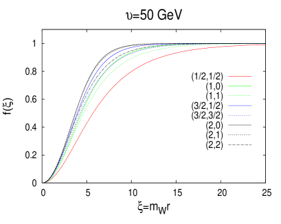
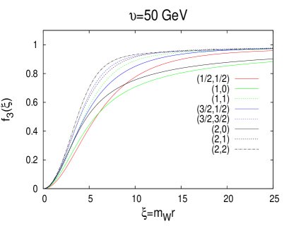
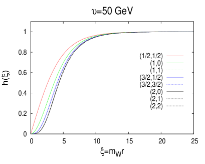
Figure 1: The field profiles $f(\xi)$, $f_{3}(\xi)$ and $h(\xi)$ as the function of the radial coordinate. In the left figures, we set the vacuum expectation value to be $v=50$ GeV and in the right, it’s $v=350$ GeV.

According to Figure 1, one can make the following remarks:

• Comparing the cases of small vev, $v=50$ GeV and large vev, $v=350$ GeV, it can be seen that all field profiles tend quickly to the unity as the vev gets larger. This could explain the dependence of sphaleron energy Eq.(17) on the scalar vev.

• When the scalar representation is large (large $J$ so that large $\alpha$), the profile for charged gauge field (i.e., $f(\xi)$) tends to $1$ faster with $\xi$, in contrast with the scalar field profile, $h(\xi)$.

• For the neutral gauge field profile $f_{3}(\xi)$, it is identical to $f(\xi)$ for the representation ($1/2,1/2$) because it satisfies $\rho=1$ (or $J(J+1)=3X^{2}$) condition.

• For the same value of the vev and the isospin $J$, the field profile $f_{3}(\xi)$ tends to 1 faster for larger values of $J_{3}$, i.e. larger values of $\beta$.

• The scalar field profiles $h(\xi)$ seem to be not sensitive to the values of $J_{3}$.

Therefore, it is seen that the gauge field profiles tend to unity faster in contrast to the scalar field profiles with radial coordinate for large couplings of the scalar to charged gauge boson, $\alpha$ and neutral gauge boson, $\beta$. In the next section, we will see the impact of this feature on the sphaleron energy.

3 The Effect of $U(1)_{X}$ Field and the Sphaleron Energy

In the presence of a non-zero $U(1)_{X}$ gauge coupling $g^{\prime}$ or non-zero Weinberg angle $\theta_{W}$, the $U(1)_{X}$ gauge field will be excited and the spherical symmetry will be reduced to axial symmetry. In Brihaye:1992jk , it was shown for the SM with one Higgs doublet that when the mixing angle is increased, the energy of the sphaleron decreases and it changes the shape from a sphere at $\theta_{W}=0$ to a very elongated spheroid at large mixing angle. However, for the physical value of the mixing angle, the sphaleron differs only little from the spherical sphaleron. On the other hand, for multiplets not satisfying Eq.(5), the shape of the corresponding sphaleron will be spheriodal instead of spherically symmetric in the $SU(2)$ case. In such cases, the large value of the mixing angle may be significant for the energy and shape of the sphaleron for large multiplet future . In the following, we have adopted the small mixing angle scenario so that $SU(2)\times U(1)_{X}$ sphalerons are not so different than the $SU(2)$ case; and we will work at first order of small $\theta_{W}$ value.

In Figure 2, we have presented the field profile $f_{0}(\xi)$ for different values of vev ($v=50,350$ GeV) and different representations ($J,X$).

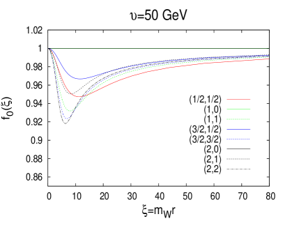
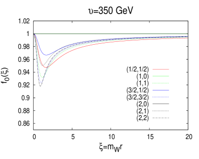
Figure 2: The field profile $f_{0}(\xi)$ as a function of the radial coordinate. In the left figure, we set the vacuum expectation value to be $v=50$ GeV and in the right, it’s $v=350$ GeV.

In the case of a $SU(2)\times U(1)_{X}$ sphaleron, we have presented only the field profile $f_{0}(\xi)$ since the other profiles ($f(\xi)$, $f_{3}(\xi)$ and $h(\xi)$) are very close to the case of vanishing Weinberg angle shown in the previous section. In Figure 2, one can notice that the field profile $f_{0}(\xi)$ is just a deviation from unity similar to the singlet scalar profile in models with singlets Ahriche:2007jp and it gets closer to unity as the $X$ values becomes smaller and smaller. Indeed, it is exactly one for the representations $(1,0)$ and $(2,0)$ which means that in those cases the sphaleron energy is not affected by the existence of $U(1)_{X}$ gauge field.

When we have $\theta_{W}\neq 0$, even when one starts with $a_{i}=0$, the following $U(1)_{X}$ current $j_{i}$ will induce $a_{i}$,

$$j_{i}=\frac{i}{2}g^{\prime}[Q^{\dagger}D_{i}Q-(D_{i}Q)^{\dagger}Q],$$ (20)

In the leading order approximation of $\theta_{W}$, we can neglect the $a_{i}$ contribution in the covariant derivative. Therefore the non-zero component of the $U(1)_{X}$ current in the chosen ansatz is Klinkhamer:1984di

$$j_{\phi}=\frac{g^{\prime}\sin\theta}{r}\sum_{i}v_{i}^{2}J_{3}^{(i)}h_{i}^{2}(1-f).$$ (21)

Because of induced field $a_{i}$, there will be a dipole contribution to the energy,

$$E_{dipole} =\int d^{3}xa_{i}j_{i}$$

$$=-\frac{16\pi}{3g\Omega}\sum_{i}v_{i}^{2}J_{3}^{(i)}\int_{0}^{\infty}d\xi(1-f_{0})(1-f)h_{i}^{2},$$ (22)

and the sphaleron energy will be

$$E_{sph}|_{\theta_{W}\neq 0}=E_{sph}|_{\theta_{W}=0}+E_{dipole}.$$ (23)

In the current Eq.(21) the contribution of the $U(1)_{X}$ gauge field is generally neglected in the literature and when we consider it, the current and the dipole energy become

$$j_{\phi} =\frac{g^{\prime}\sin\theta}{r}\sum_{i}v_{i}^{2}J_{3}^{(i)}h_{i}^{2}(f_{0}-f_{3}),$$

$$E_{dipole}^{\prime} =-\frac{16\pi}{3g\Omega}\sum_{i}v_{i}^{2}J_{3}^{(i)}\int_{0}^{\infty}d\xi(1-f_{0})(f_{0}-f_{3})h_{i}^{2},$$ (24)

Therefore the dipole contribution Eq.(22) is expected to be almost equal to the difference between Eq.(17) and the same quantity with $g^{\prime}=0$, i.e., $E_{dipole}\simeq\Delta E_{sph}=E_{sph}(g^{\prime}\neq 0)-E_{sph}(g^{\prime}=0)$. In order to probe this, we estimate the difference between the sphaleron energy in the non-zero and zero mixing cases in three different ways: (A) $\Delta E_{sph}=E_{sph}(g^{\prime}\neq 0)-E_{sph}(g^{\prime}=0)$ with $E_{sph}$ is given in Eq.(17); (B) $\Delta E_{sph}=E_{dipole}$ with $U(1)_{X}$ field neglected as given in Eq.(22); and (C) $\Delta E_{sph}=E_{dipole}^{\prime}$ as shown in Eq.(24). These three quantities are presented in function of the scalar vev in Figure 3.

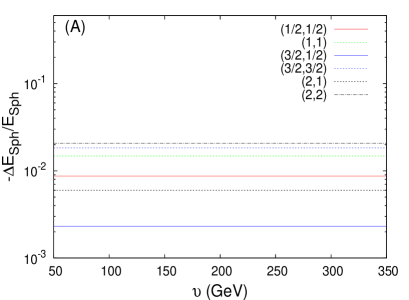
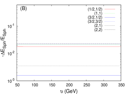
Figure 3: The relative difference in the sphaleron energy between the non-zero and zero mixing cases versus the scalar vev for different scalar representations, where the difference is estimated: exactly (left), using the dipole approximation with $U(1)$ gauge field effect neglected, Eq.(22) (right), and the case with $U(1)$ gauge field effect considered, Eq.(24) (down)

Figure 3 shows the relative difference between the sphaleron energy with the mixing angle $\theta_{W}\neq 0$ and $\theta_{W}=0$ and also the (negative) dipole energy of the sphaleron. It turns out that for any scalar representation, the relative difference between the sphaleron energy with $\theta_{W}\neq 0$ and $\theta_{W}=0$ is always less than $1\%$ and remains constant for different values of scalar vev. However, when considering the $U(1)_{X}$ gauge field effect on the dipole energy Eq.(24), it becomes closer to the exact difference.

Now we present the sphaleron energy Eq.(17) as a function of the scalar vev for different scalar representations as shown in Figure 4.

Figure 4: The sphaleron energy versus the scalar vev for different scalar representations.

In Figure 4 we can see that the sphaleron energy depends on the scalar vev with a slope that depends on scalar isospin $J$ and hypercharge $X$ (or $J_{3}$). This allows us the write the scaling law as

$$E_{sph}(v,J,X)=Z(J,X)\,v,$$ (25)

where the function $Z(J,X)$ represents the slope in Figure 4.

4 Sphaleron Decoupling Condition

Before the electroweak phase transition $T>T_{c}$, the classical background scalar field, $\phi_{c}$, is zero and the Universe is in the symmetric phase. In this phase, the sphaleron processes are in full thermal equilibrium and are given as Arnold:1996dy ; Bodeker:1998hm ; Arnold:1998cy ; Moore:2000mx

$$\Gamma_{sym}\sim\alpha_{w}^{5}T^{4}\ln(1/\alpha_{w}),$$ (26)

with $\alpha_{w}=g^{2}/4\pi$ is the weak coupling. Therefore any generated baryon asymmetry due to the sphaleron processes will be erased by the inverse process. Once the temperature drops below the critical one $T<T_{c}$, bubbles of true vacuum ($\phi_{c}\neq 0$) start to nucleate where the rate is suppressed as $\Gamma\sim\exp\left(-E_{sph}/T\right)$.

The sphaleron decoupling condition indicates that the rate of baryon number violation must be much smaller than the the Hubble parameter Shaposhnikov:1987tw ; Shaposhnikov:1987pf ; Bochkarev:1987wf and therefore, the condition on the sphaleron rate is Arnold:1987mh ; Akiba:1989xu ; Funakubo:2009eg

$$-\frac{1}{B}\frac{dB}{dt}\simeq\frac{13N_{f}}{128\pi^{2}}\frac{\omega_{-}}{\alpha_{w}^{3}}\kappa{\mathcal{N}_{tr}}{\mathcal{N}_{rot}}e^{-E_{sph}/T}<H(T),$$ (27)

where $B$ is the baryon number density, the factors $N_{tr}~{}$and $N_{rot}$ come from the zero mode normalization, $\omega_{-}$ is the eigenvalue of the negative mode Carson:1989rf . The factor $\kappa$ is the functional determinant associated with fluctuations around the sphaleron Dine:1991ck . It has been estimated to be in the range: $10^{-4}\lesssim\kappa\lesssim 10^{-1}$ Carson:1990jm ; kapan . The Hubble parameter is given as

$$H(T)\simeq 1.66\sqrt{g_{\ast}(T)}T^{2}/M_{pl},$$ (28)

where $M_{pl}$ and $g_{\ast}$ are the Planck mass and the effective number of degrees of freedom that are in thermal equilibrium.

It was shown in Braibant:1993is for the doublet case $(J,X)=(1/2,1/2)$ that the sphaleron energy at a given temperature can be well approximated by the following relation

$$\frac{E_{sph}(v(T),T)}{v(T)}=\frac{E_{sph}(v_{0})}{v_{0}},$$ (29)

where $v(T)$ is the vev of the scalar field at temperature $T$ and $v_{0}$ is its zero temperature value. Eq.(29) shows that a straightforward estimation of the sphaleron energy at finite temperature is possible by determining its energy at zero temperature. This means that the scaling law Eq.(25) is valid also at finite temperature case, where the function $Z(J,X)$ is temperature-independent. Because of similar linear scaling shown by higher scalar representations in Figure 4, we can use the scaling law Eq.(25) for other representations.

Hence, for general scalar representation, the decoupling of baryon number violation Eq.(27) implies the following relation Funakubo:2009eg

$$\frac{v(T_{c})}{T_{c}}>\frac{1}{Z(J,X)}\left[42.97+\ln(\kappa{\mathcal{N}_{tr}}{\mathcal{N}_{rot}})+\ln\tfrac{\omega_{-}}{m_{W}}-\tfrac{1}{2}\ln\tfrac{g_{\ast}}{106.75}-2\ln\tfrac{T_{c}}{100\text{ {\normalsize{GeV }}}}\right].$$ (30)

Most of the parameters in the r.h.s of Eq.(30) are logarithmically model-dependent and therefore one can safely use the SM values. In the case of SM, we have $\mathcal{N}_{tr}\mathcal{N}_{rot}\simeq 80.13$ Arnold:1987mh and for $\lambda/g^{2}=1$, $\omega_{-}^{2}\simeq 2.3m_{W}^{2}$ Carson:1989rf ; Carson:1990jm ; Akiba:1989xu . It can be noted that the contributions of model dependent quantities in $v(T)/T$ are smaller than $Z(J,X)$, for example, in the SM Funakubo:2009eg zero mode contribution is around $10\%$ and the contributions from the negative mode, relativistic degrees of freedom and critical temperature are about $1\%$. For this reason we can consider the dominant contribution is coming from $Z(J,X)$. In conjunction, using $\kappa=10^{-1}$ (or $10^{-4}$), $g_{\ast}\simeq 106.75$ and $T_{c}\simeq 100$ GeV, we have from Eq.(30),

$$\frac{v(T_{c})}{T_{c}}>\eta_{J,X},$$ (31)

where $\eta_{J,X}$ is given for each scalar representation in Table-1.

$J$	$X$	$Z(J,X)$	$\eta_{J,X}\left(\kappa=10^{-4}\right)$		$\eta_{J,X}\left(\kappa=10^{-1}\right)$
1/2	1/2	36.37	$\allowbreak 1.0601$		$1.2500$
1	0	44.64	$0.8639$		$1.0186$
	1	45.37	$\allowbreak 0.8500$		$1.0023$
3/2	1/2	50.89	$\allowbreak 0.7577$		$0.8934$
	3/2	50.42	$\allowbreak 0.7648$		$\allowbreak 0.9018$
2	0	53.58	$0.7197$		$0.8486$
	1	55.22	$\allowbreak 0.6984$		$\allowbreak 0.8235$
	2	53.80	$\allowbreak 0.7167$		$\allowbreak 0.8451$

Table 1: The values for the parameters $Z(J,X)$ and $\eta_{J,X}$ for different scalar representations.

It is clear that as the representation becomes larger, the strong first order phase transition criterion gets relaxed. Generally, the case of $\kappa=10^{-4}$ is the commonly used criterion in the literature. In a general case of a multi-scalars model with representations ($J^{(i)},X^{(i)}$), the criterion Eq.(31) can be generalized as

$$\frac{\Theta(T_{c})}{T_{c}}>1,$$ (32)

with

$$\Theta(T_{c})^{2}=\sum\limits_{i}\frac{v_{i}(T_{c})^{2}}{\eta_{J^{(i)},X^{(i)}}^{2}},$$ (33)

with $v_{i}(T)$ is the temperature dependent scalar vev of the multiplet $Q^{(i)}$. In order to check the criterion Eq.(33), we consider the case of a model with two scalar representations and estimate the ratio $E_{sph}/\Theta$ for different values of $J_{1}$, $J_{2}$, $X_{1}$, $X_{2}$, $v_{1}$ and $v_{2}$ while keep the W gauge boson mass constant. The ratio $E_{sph}/\Theta$ versus the ratio $v_{2}/v_{1}$ is shown in Figure 5.

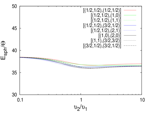
Figure 5: The sphaleron energy versus the scalar vev for different scalar representations. The self quartic couplings of scalar multiplet $Q_{1}(J_{1},X_{1})$ ($Q_{2}(J_{2},X_{2})$) is set to $0.12$ ($0.06$) while the mixing quartic coupling is set to $0.02$.

From Figure 5, it is clear that the sphaleron energy scales like $\Theta$ for different representations and vevs within the error less than 5.7 %; and if the values of the two vevs are comparable, this error is reduced to 2.7 %. Therefore, one can safely use Eq.(33) as a criterion for a strong first order phase transition in any model with multiscalars.

5 Conclusion

We have constructed the energy functional and relevant variational equations of the sphaleron for general scalar representation charged under $SU(2)\times U(1)_{X}$ gauge group and shown that the sphaleron energy increases with the size of the multiplet. Furthermore, it has been shown that at a fixed value of the vev, the sphaleron energy is large for larger representation and for each representation, it linearly scales with the vev. As the energy of the sphaleron increases with the size of the scalar representation, the criterion for the strong first order phase transition is relaxed for larger representation. We have presented a representation dependent criterion for strong phase transition which is relevant for the electroweak baryogenesis.

We have also found that the dipole approximation (with or without considering $a_{i}$ in the $U(1)_{X}$ current, $j_{i}$) does not correspond exactly the energy difference $E_{sph}(g^{\prime}\neq 0)-E_{sph}(g^{\prime}=0)$ and that is less than 2% for any scalar representation. In this case the $U(1)_{X}$ field profile is just a deviation from unity and therefore just playing a relaxing role similar to singlet seen in Ahriche:2007jp .

However, as we have seen in Figure 3 that the dipole contribution to the sphaleron energy is negative, its coupling with the external magnetic field produced in the bubbles of first order phase transition through the dipole moment would lower the sphaleron energy and thus strengthen the sphaleron transition inside the bubble and wash out the baryon asymmetry more efficiently as pointed out in DeSimone:2011ek . A more careful analysis on this aspect for the sphaleron with higher scalar representation will be carried out in future .

We have presented in Eq.(33) a general criterion for the strong first order phase transition in a model with multiple scalars of different representations $(J,X)$ and we have shown that this approximate criterion is valid with an error less than 5%.

Appendix A Asymptotic solutions

To capture the dependence of solutions on $(J,X)$, in this section we have included the analytical estimates of solutions for the asymptotic region $\xi\rightarrow 0$ and $\xi\rightarrow\infty$. For the energy functional Eq.(17) to be finite, the profile functions should be $f(\xi)\rightarrow 0$, $f_{3}(\xi)\rightarrow 0$, $f_{0}(\xi)\rightarrow 1$ and $h(\xi)\rightarrow 0$. Therefore, at $\xi\sim 0$, the equations Eq.(19) are reduced into

$$\xi^{2}f^{\prime\prime} -4f+2f_{3}+\alpha\xi^{2}h^{2}=0,$$ (34)

$$\xi^{2}f_{3}^{\prime\prime} -6f_{3}+4f+\beta\xi^{2}h^{2}=0,$$ (35)

$$f_{0}^{\prime\prime} +2(1-f_{0})-(\frac{g^{\prime}}{g})^{2}\beta\xi^{2}h^{2}=0,$$ (36)

$$\xi^{2}h^{\prime\prime} +2\xi h^{\prime}-\frac{8m}{3}h=0,$$ (37)

where

$$m=\frac{\Omega^{2}}{v^{2}}(2\alpha+\beta).$$ (38)

The solution of Eq.(37) which leads to finite energy of the sphaleron is

$$h(\xi)\sim A\xi^{-\frac{1}{2}(1-p)},$$ (39)

with

$$p=\sqrt{1+\frac{32}{3}m}.$$ (40)

Now at $\xi\sim 0$, $f(\xi)\sim f_{3}(\xi)$, so using this approximation, from Eq.(34) we have,

$$f(\xi)\sim B\xi^{2}-\frac{4A\alpha\xi^{\frac{1}{2}(3+p)}}{(\frac{p}{2}-1)(\frac{p}{2}+5)}.$$ (41)

On the other hand, we have considered $f(\xi)$ as a perturbation in Eq.(35). Therefore, we have

$$f_{3}(\xi)\sim C\xi^{3}+B\xi^{2}-K\xi^{\frac{1}{2}(3+p)}.$$ (42)

Here, $K$ is defined as follows

$$K=\frac{3A\{3\alpha(3p-8m+3)+8m\beta(4m-9)\}}{4m(4m-9)(8m+3p-15)}.$$ (43)

Finally from Eq.(36), we have

$$f_{0}(\xi)\sim 1+D\xi^{2}+\frac{3A\beta g^{\prime 2}\xi^{\frac{1}{2}(3+p)}}{g^{2}(3p-8m+3)},$$ (44)

and $A$, $B$, $C$ and $D$ are integration constants.

On the other hand, for asymptotic region, $\xi\sim\infty$, all the profile functions must approach unity to have finite energy of the sphaleron. So we consider the functions to be the small perturbation to unity as follows. Taking, $f(\xi)=1+\delta f(\xi)$, $f_{3}(\xi)=1+\delta f_{3}(\xi)$, $f_{0}(\xi)=1+\delta f_{0}(\xi)$ and $h(\xi)=1+\delta h(\xi)$ and keeping only the linear terms of the variation, we have

$$\delta f^{\prime\prime}-\alpha\delta f =0,$$

$$\delta f_{3}^{\prime\prime}+\beta(\delta f_{0}-\delta f_{3}) =0,$$

$$\delta f_{0}^{\prime\prime}-\frac{g^{\prime 2}}{g^{2}}\beta(\delta f_{0}-\delta f_{3}) =0,$$

$$\xi^{2}\delta h^{\prime\prime}-2\xi\delta h-3\frac{\lambda v^{2}}{g^{2}\Omega^{2}}\xi^{2}\delta h =0.$$ (45)

The asymptotic solutions at $\xi\sim\infty$ are,

$$f(\xi) \sim 1+Ee^{-\sqrt{\alpha}\xi},$$

$$f_{3}(\xi) \sim 1+Fe^{-\sqrt{\beta}\xi},$$

$$f_{0}(\xi) \sim 1+Ge^{-\sqrt{\beta}\xi},$$

$$h(\xi) \sim 1+\frac{He^{-\frac{\sqrt{3\lambda}v}{g\Omega}\xi}}{\xi},$$ (46)

where $E$, $F$, $G$ and $H$ are again integration constants. The constants from $A$ to $H$ depend on $(J,X)$ and couplings and they are determined by matching the corresponding asymptotic solutions and their first derivatives at $\xi=0$. Therefore after the matching, the integration constants are,$v_{1}$ and $v_{2}$

$$H =-\frac{\frac{1}{2}(p-1)e^{\frac{v}{\Omega}n}}{\frac{1}{2}(p+1)+\frac{v}{\Omega}n},~{}A=1+He^{-\frac{v}{\Omega}n},$$

$$E =-\frac{e^{\sqrt{\alpha}}}{\sqrt{\alpha}+2}(2+\frac{2A\alpha(1-p)}{(\frac{p}{2}-1)(\frac{p}{2}+5)}),~{}B=1+Ee^{-\sqrt{\alpha}}+\frac{4A\alpha}{(\frac{p}{2}-1)(\frac{p}{2}+5)},$$

$$B =1+Ee^{-\sqrt{\alpha}}+\frac{4A\alpha}{(\frac{p}{2}-1)(\frac{p}{2}+5)},~{}F=\frac{e^{\sqrt{\beta}}}{\sqrt{\beta}+3}(-3+B-\frac{1}{2}(3-p)K),$$

$$C =1+Fe^{-\sqrt{\beta}}-B+K,~{}G=\frac{e^{\sqrt{\beta}}}{\sqrt{\beta}+2}\frac{3A\beta n_{1}^{2}(1-p)}{2(3p+8m-3)},$$

$$D =Ge^{-\sqrt{\beta}}-\frac{3A\beta n_{1}^{2}}{3p+8m-3},$$ (47)

where $n=\sqrt{3\lambda}/g$, where $\lambda$ is the scalar quartic coupling.

References

- (1) G. ’t Hooft, Phys. Rev. Lett. 37 (1976) 8.
- (2) G. ’t Hooft, Phys. Rev. D 14 (1976) 3432 [Erratum-ibid. D 18 (1978) 2199].
- (3) R. F. Dashen, B. Hasslacher and A. Neveu, Phys. Rev. D 10 (1974) 4138.
- (4) N. S. Manton, Phys. Rev. D 28 (1983) 2019.
- (5) F. R. Klinkhamer and N. S. Manton, Phys. Rev. D 30 (1984) 2212.
- (6) V. Soni, Phys. Lett. B 93 (1980) 101.
- (7) V. A. Kuzmin, V. A. Rubakov and M. E. Shaposhnikov, Phys. Lett. B 155 (1985) 36.
- (8) M. E. Shaposhnikov, Nucl. Phys. B 287 (1987) 757.
- (9) M. E. Shaposhnikov, Nucl. Phys. B 299 (1988) 797.
- (10) P. B. Arnold and L. D. McLerran, Phys. Rev. D 36, 581 (1987).
- (11) S. Y. .Khlebnikov and M. E. Shaposhnikov, Nucl. Phys. B 308 (1988) 885.
- (12) M. Dine, O. Lechtenfeld, B. Sakita, W. Fischler and J. Polchinski, Nucl. Phys. B 342 (1990) 381.
- (13) M. Dine, P. Huet and R. L. Singleton, Jr., Nucl. Phys. B 375 (1992) 625.
- (14) T. Akiba, H. Kikuchi and T. Yanagida, Phys. Rev. D 38 (1988) 1937.
- (15) T. Akiba, H. Kikuchi and T. Yanagida, Phys. Rev. D 40 (1989) 588.
- (16) L. G. Yaffe, Phys. Rev. D 40 (1989) 3463.
- (17) P. B. Arnold and L. D. McLerran, Phys. Rev. D 37 (1988) 1020.
- (18) L. Carson, X. Li, L. D. McLerran and R. -T. Wang, Phys. Rev. D 42 (1990) 2127.
- (19) F. R. Klinkhamer and R. Laterveer, Z. Phys. C 53 (1992) 247.
- (20) B. Kleihaus, J. Kunz and Y. Brihaye, Phys. Lett. B 273 (1991) 100.
- (21) J. Kunz, B. Kleihaus and Y. Brihaye, Phys. Rev. D 46 (1992) 3587.
- (22) Y. Brihaye, B. Kleihaus and J. Kunz, Phys. Rev. D 47 (1993) 1664.
- (23) S. Braibant, Y. Brihaye and J. Kunz, Int. J. Mod. Phys. A 8 (1993) 5563 [hep-ph/9302314].
- (24) Y. Brihaye and J. Kunz, Phys. Rev. D 48 (1993) 3884 [hep-ph/9304256].
- (25) J. Choi, Phys. Lett. B 345 (1995) 253 [hep-ph/9409360].
- (26) A. Ahriche, Phys. Rev. D 75 (2007) 083522 [hep-ph/0701192].
- (27) B. M. Kastening, R. D. Peccei and X. Zhang, Phys. Lett. B 266 (1991) 413.
- (28) J. M. Moreno, D. H. Oaknin and M. Quiros, Nucl. Phys. B 483 (1997) 267 [hep-ph/9605387].
- (29) K. Funakubo, A. Kakuto, S. Tao and F. Toyoda, Prog. Theor. Phys. 114 (2006) 1069 [hep-ph/0506156].
- (30) A. Ahriche, Eur. Phys. J. C 66 (2010) 333 [arXiv:0904.0700 [hep-ph]].
- (31) H. Georgi and M. Machacek, Nucl. Phys. B 262 (1985) 463.
- (32) S. Kanemura, M. Kikuchi and K. Yagyu, Phys. Rev. D 88 (2013) 1, 015020 [arXiv:1301.7303 [hep-ph]].
- (33) S. S. AbdusSalam and T. A. Chowdhury, JCAP 1405 (2014) 026 [arXiv:1310.8152 [hep-ph]].
- (34) K. Hally, H. E. Logan and T. Pilkington, Phys. Rev. D 85, 095017 (2012) [arXiv:1202.5073 [hep-ph]].
- (35) K. Earl, K. Hartling, H. E. Logan and T. Pilkington, arXiv:1303.1244 [hep-ph].
- (36) M. Blennow, B. Dasgupta, E. Fernandez-Martinez and N. Rius, JHEP 1103 (2011) 014 [arXiv:1009.3159 [hep-ph]].
- (37) S. M. Barr and H. -Y. Chen, JHEP 1310 (2013) 129 [arXiv:1309.0020 [hep-ph]].
- (38) A. Ahriche, T. A. Chowdhury and Salah Nasri, in preparation.
- (39) P. B. Arnold, D. Son and L. G. Yaffe, Phys. Rev. D 55 (1997) 6264 [hep-ph/9609481].
- (40) D. Bodeker, Phys. Lett. B 426, 351 (1998) [hep-ph/9801430].
- (41) P. B. Arnold, D. T. Son and L. G. Yaffe, Phys. Rev. D 59, 105020 (1999) [hep-ph/9810216].
- (42) G. D. Moore, Phys. Rev. D 62 (2000) 085011 [hep-ph/0001216].
- (43) A. I. Bochkarev and M. E. Shaposhnikov, Mod. Phys. Lett. A 2 (1987) 417. A. I. Bochkarev, S. V. Kuzmin and M. E. Shaposhnikov, Phys. Rev. D 43 (1991) 369.
- (44) K. Funakubo and E. Senaha, Phys. Rev. D 79 (2009) 115024 [arXiv:0905.2022 [hep-ph]]; K. Fuyuto and E. Senaha, Phys. Rev. D 90, 015015 (2014) [arXiv:1406.0433 [hep-ph]].
- (45) L. Carson and L. D. McLerran, Phys. Rev. D 41 (1990) 647.
- (46) J. Baake and S. Junker, Phys. Rev. D49 (1994) 2055 [hep-ph/9308310]; Phys. Rev. D50 (1994) 67 [hep-th/9402078].
- (47) A. De Simone, G. Nardini, M. Quiros and A. Riotto, JCAP 1110 (2011) 030 [arXiv:1107.4317 [hep-ph]].