The rich complexity of 21-cm fluctuations produced by the first stars

Abstract

We explore the complete history of the 21-cm signal in the redshift range $z=7-40$. This redshift range includes various epochs of cosmic evolution related to primordial star formation, and should be accessible to existing or planned low-frequency radio telescopes. We use semi-numerical computational methods to explore the fluctuation signal over wavenumbers between 0.03 and 1 Mpc^-1, accounting for the inhomogeneous backgrounds of Ly$\alpha$, X-ray, Lyman-Werner and ionizing radiation. We focus on the recently noted expectation of heating dominated by a hard X-ray spectrum from high-mass X-ray binaries. We study the resulting delayed cosmic heating and suppression of gas temperature fluctuations, allowing for large variations in the minimum halo mass that contributes to star formation. We show that the wavenumbers at which the heating peak is detected in observations should tell us about the characteristic mean free path and spectrum of the emitted photons, thus giving key clues as to the character of the sources that heated the primordial Universe. We also consider the line-of-sight anisotropy, which allows additional information to be extracted from the 21-cm signal. For example, the heating transition at which the cosmic gas is heated to the temperature of the cosmic microwave background should be clearly marked by an especially isotropic power spectrum. More generally, an additional cross-power component $P_{X}$ directly probes which sources dominate 21-cm fluctuations. In particular, during cosmic reionization (and after the just-mentioned heating transition), $P_{X}$ is negative on scales dominated by ionization fluctuations and positive on those dominated by temperature fluctuations.

1 Introduction

Critical stages of the evolution of our Universe still remain a mystery due to the lack of direct observational probes. This includes the cosmic dark ages, the formation era of the first stars and black holes, the early heating and metal enrichment of the intergalactic medium (IGM), and the epoch of reionization. A crucial step in the evolution of the Universe is the formation of first stars. In fact, to start forming stars in the pristine chemical conditions of the early Universe, gas has to be gravitationally accelerated at least to the temperature of $T\lower 2.15277pt\hbox{$\;\buildrel>\over{\sim}\;$}300$ K to initiate the radiative cooling process (for comparison, atomic hydrogen radiatively cools when it reaches $T\sim 10^{4}$ K). Since the cooling temperature of molecular hydrogen is so low, stars can form even in light halos of mass $\sim 10^{5}$ M_⊙ (Tegmark et al., 1997; Haiman, Thoul & Loeb, 1996; Machacek, Bryan & Abel, 2010; Abel, Bryan & Norman, 2002). The first stars emitted radiation, in particular photons in the Lyman-Werner (LW) band (11.2-13.6 eV), which dissociate molecular hydrogen, leading to a suppression of star formation. As a result of this negative feedback, larger halos were needed to accelerate gas enough so that it can radiatively cool, condense and form stars (Machacek, Bryan & Abel, 2010; Wise & Abel, 2000; O’Shea & Norman, 2000; Haiman, Abel & Rees, 2000). The effect of a time-dependent LW background is still highly unconstrained given the current state of observations and simulations. A first study in a recent numerical simulation (Visbal et al., 2014) suggests that the effect of LW radiation may be fast, leading to a relatively strong suppression of H₂-based star formation early in cosmic history. An additional suppression of star formation via cooling of molecular hydrogen is due to the supersonic relative velocity ($v_{\rm bc}$) between dark matter and gas (Tseliakhovich & Hirata, 2010).

During its early evolution (before the epoch of reionization) the Universe remained overall neutral with atomic hydrogen being the most abundant element. This should allow the probing of most of the as-yet unobserved stages of cosmic history using lines of hydrogen, in particular its 21-cm line (Van der Hulst, 1945) which corresponds to the hyper-fine splitting of the H I ground state. This line, despite its low optical depth, can in principle be observed today using ground-based or space and lunar telescopes, allowing us to complete our knowledge of cosmic history. In fact, many of the low-frequency radio observatories in place today are after this “holy grail”. This includes the Low Frequency Array [LOFAR] (van Haarlem, 2013), the Murchison Wide-field Array [MWA] (Bowman et al., 2013), the Giant Meterwave Radio Telescope [GMRT] (Paciga et al., 2013), the Long Wavelength Array [LWA] (Ellingson et al., 2013), and the Precision Array to Probe the Epoch of Reionization [PAPER] (Parsons et al., 2010). These instruments are mainly focused on measuring the 21-cm signal from the Epoch of Reionization around $z\sim 10$. Future observatories, including the Square Kilometer Array [SKA] (Mellema et al., 2013), Hydrogen Epoch of Reionization Array [HERA] (Pober et al., 2014) and the Dark Ages Radio Explorer [DARE] (Burns et al., 2012) will likely be designed to observe the redshifted 21-cm signal from higher redshifts. The design of the next generation experiments as well as interpretation of data from the telescopes that are currently making observations, rely on our theoretical understanding of the expected signal. Modeling of the 21-cm signal from high redshifts is technically very challenging, and it is a rapidly evolving field. For instance, the global spectrum and the power spectrum of the expected 21-cm signal was recently shown to be very sensitive to the spectral energy distribution (SED) of X-rays emitted by the first heating sources (Fialkov et al., 2014).

The origin of the heating sources at high redshifts is still largely uncertain. High-mass X-ray binaries (HMXBs) are thought to be the most likely driver of cosmic heating, the idea (Mirabel et al., 2011) supported by current observations and a recent detailed population synthesis simulation of X-ray binaries (Fragos et al., 2013) that found that HMXBs likely dominate over the contribution of quasars at $z\gtrsim 6-8$. This work was calibrated to all available low-redshift X-ray observations and yielded X-ray spectra which peak at $\sim 3$ keV and have an almost redshift-independent shape. On the other hand, the overall normalization of the spectral energy distribution (SED) changes by an order of magnitude due to the changing metallicity, and also roughly tracks the evolving cosmic star formation rate. Fragos et al. (2013) provides a reasonable framework to study the effect of X-ray binaries on cosmic history, as in Fialkov, Barkana & Visbal (2014). The probable dominance of HMXBs as the early heating sources is also (indirectly) supported by numerical simulations that show that the first stars were massive and likely formed in groups due to fragmentation (e.g., see the review by Bromm (2013) and references therein). Such systems of multiple heavy stars are likely to evolve into HMXBs.

Other possible heating sources are thermal emission from hot gas in galaxies (Mineo, Gilfanov & Sunyaev, 2012; Pacucci et al., 2014) and Compton emission from relativistic electrons (Oh, 2001), which are likely subdominant at high redshift (Fialkov, Barkana & Visbal, 2014). Specifically, in observed galaxies the X-ray energy from hot gas is lower than that from X-ray binaries by a factor of several; at high redshifts, the higher heating efficiency of soft X-rays (as expected from hot gas) could compensate for this, but the order of magnitude increase in X-rays from X-ray binaries at the low metallicities of early galaxies would have to be compensated by a similar increase in the hot gas emission. More promising is the possibility of X-rays from a population of mini-quasars, i.e., central black holes in early star-forming halos. The properties of these objects are highly unconstrained, so in principle they could produce either early or late heating (Tanaka, Perna & Haiman, 2012; Ciardi, Salvaterra & Di Matteo, 2013); observationally-based estimates suggest that mini-quasars are also likely subdominant (see Methods in Fialkov, Barkana & Visbal (2014)). Heating by shocks due to structure formation at high redshifts is also unlikely to be important (Furlanetto & Loeb, 2004), even after being enhanced by supersonic relative motion between the gas and dark matter (McQuinn & O’Leary, 2013). Some more exotic scenarios have also been suggested, including heating by evaporating black holes (Ricotti, Ostriker & Mack, 2008), cosmic strings (Brandenberger et al., 2010), or dark matter annihilation (Valdes et al., 2013). In any case, our results also act as an illustration of the more general idea of how the properties of cosmic heating sources can be probed with 21-cm observations.

Despite the plethora of possible heating sources, the effect of inhomogeneous X-rays has not been studied in simulations of reionization. Due to the historical evolution of the field (Madau, Meiksin & Rees, 1997; Furlanetto, Oh & Briggs, 2006; Furlanetto, 2006), many of the present state-of-the-art simulations of reionization, which include precise radiative transfer for ionizing photons, neglect the role of an inhomogeneous X-ray background. For instance, some simulations (e.g., Iliev et al. (2014)) assume heating to be saturated during reionization, i.e., that the gas is much hotter than the Cosmic Microwave Background (CMB), in which case X-rays do not have an impact on the 21-cm signal (except in the unlikely case that they contribute substantially to reionization). Saturated heating is also usually assumed in analyses of current and future observations of cosmic reionization (Patil et al., 2014; Pober et al., 2014). Some simulations do treat the radiative transfer of X-rays (Baek et al., 2010; Zawada et al., 2014), but they do not include X-ray binaries as sources, with one reasonable argument being that the mean free path of those hard X-rays would be larger than their simulation box. In addition, most semi-numerical, hybrid methods, which are capable of making predictions for the 21-cm signal on very large scales (e.g., Mesinger, Furlanetto & Cen (2011); Visbal et al. (2012); Fialkov et al. (2013, 2014)), used a soft power-law spectrum for X-ray emission motivated by Furlanetto (2006) who used the results of Rephaeli (1995). However, more recent work suggests that the power-law spectrum does not describe well the observed or expected X-ray emission by HMXBs, which as mentioned above are probably the main X-ray sources within starburst galaxies.

Motivated by the necessity to better model the effect of X-rays on the 21-cm signal as discussed above, we estimated the impact of the X-ray SED on the reionization era ($z=7-16$) in our previous paper (Fialkov et al., 2014). In this work one of our main goals is to extend the redshift range and to explore the impact of a hard versus soft X-ray SED on the 21-cm signal from $z=7-40$, which now includes the redshifts at which the effect of X-rays is expected to be maximal ($z\sim 17-20$). A second main point of emphasis in this paper is on the line-of-sight anisotropy of the 21-cm signal due to the gradient of the gas velocity. This anisotropy adds some overall power to the 21-cm fluctuations (Bharadwaj & Ali, 2004), but more importantly, it allows several power spectrum components to be separately measured, in principle allowing much more information to be extracted about the various sources of 21-cm fluctuations (Barkana & Loeb, 2005a). We note that the line-of-sight anisotropy has been previously studied during reionization (Mesinger, Furlanetto & Cen, 2011; Mao et al., 2012; Shapiro et al., 2013; Majumdar et al., 2013), but we discuss it over a wide redshift range that includes various cosmic epochs. Finally, we make sure to sample a wide range of parameters. Specifically, we analyze several cases of possible star-formation histories, considering three main cases of star-forming halos including the molecular cooling case with time-dependent LW feedback and with the velocity streaming effect, the atomic cooling case, and the third case in which stars form only in massive halos (M${}_{h}\gtrsim 10^{8}$ M_⊙).

This paper is organized as follows: In section 2 we briefly discuss our model, including technical aspects of the methods applied in this paper. We then present and discuss our results for the cosmic heating history and the 21-cm signal in section 3. Finally, we summarize our conclusions in section 4.

2 Model and Computational Methods

In this paper, we use semi-numerical computational methods (Mesinger, Furlanetto & Cen, 2011; Fialkov, Barkana & Visbal, 2014) to efficiently and self-consistently generate histories of the 21-cm signal in $\sim 400$ Mpc³ volumes, applying a sub-grid model to each 3 Mpc pixel. We assume periodical boundary conditions and perform the spatial integrations in Fourier space, which allows us to also account for radiation with mean free paths larger than the box size. In the calculation, large scale structure is tracked from $z\sim 60$, just after the first stars are expected to form (Naoz, Noter & Barkana, 2006; Fialkov et al., 2012), to $z\sim 7$ when neutral gas is completely reionized; specifically, we assume a total optical depth to reionization of $\tau=0.075$, our “late” reionization case from Fialkov, Barkana & Visbal (2014) which is motivated by various observations (Bennett et al., 2013; Ade et al., 2013; Schroeder, Mesinger, & Haiman, 2013). Simultaneously we evolve three-dimensional cubes of inhomogeneous X-ray, Ly$\alpha$, and LW radiative backgrounds as well as the ionized fraction of gas (accounting for the partial ionization by X-rays in regions not yet reionized by stellar ultra-violet photons). We average all our results over six data cubes with different randomly generated realizations of the initial conditions for density and relative velocity fields. This averaging brings us closer to expected real measurements since the field of view in realistic observations is significantly larger than even our fairly large box size.

Following Fialkov, Barkana & Visbal (2014), we further explore the impact of the realistic hard X-ray power spectrum on the 21-cm signal, expanding the redshift range to $7<z<40$. We compare the 21-cm signal in the case of gas heated by sources with the soft (previously conventional) power-law X-ray spectrum to the case of gas heated by a realistic population of X-ray binaries. We consider three possible histories of star-forming halo populations: (1) “massive halos”, which assumes that stars form in halos with circular velocities above $V_{c}=35$ km s^-1 ($M\gtrsim 3\times 10^{8}M_{\odot}$ at $z=20$), an example of the case where lower-mass halos are inefficient at star formation, e.g., due to internal feedback from supernovae or a mini-quasar; (2) “atomic cooling halos”, in which the minimum mass for cooling and star formation is set by the need for atomic hydrogen to be radiatively cooled, i.e., $V_{c}=16.5$ km s^-1 and above ($M\gtrsim 3\times 10^{7}M_{\odot}$ at $z=20$); (3) “molecular cooling halos” - halos with masses down to the minimum halo mass in which stars form through molecular cooling, i.e., $V_{c}\gtrsim 4$ km s^-1 ($M\gtrsim 7\times 10^{5}M_{\odot}$ at $z=20$ if there were no feedback). We add this third case since we are considering a broad redshift range including very early times in which the smallest halos may have dominated star formation.

In the molecular cooling case, the population of halos is suppressed by the negative feedback of the Lyman-Werner (LW) photons; motivated by the simulation results of (Visbal et al., 2014), we assume the “strong” LW feedback case from Fialkov et al. (2013) and Fialkov et al. (2014). In addition, these light halos suffer significantly from the effect of the relative velocity $v_{\rm bc}$, which includes a suppression of halo abundance and gas fraction, and an increase in the minimal cooling mass (e.g., Tseliakhovich & Hirata (2010); Dalal, Pen & Seljak (2010); Tseliakhovich, Barkana & Hirata (2011); Greif et al. (2011); Stacy, Bromm & Loeb (2011); Fialkov et al. (2012)). We use our semi-numerical methods (Visbal et al., 2012; Fialkov et al., 2012, 2013, 2014) to include these effects as we evolve in the same framework the large-scale distribution of stars and the radiative backgrounds emitted by these stars. We use the standard set of cosmological parameters (Ade et al., 2013), a star formation efficiency of $f_{*}=0.05\%$ (with additional log(M) suppression at small masses (Machacek, Bryan & Abel, 2010)) for the case of the molecular cooling halos, $f_{*}=0.05\%$ for the case of the atomic cooling halos and $f_{\star}=0.15\%$ for the massive halos. In each case $f_{*}$ is chosen so that the escape fraction of ionizing photons would need to be $\sim 20\%$ for a reionization history with our assumed total optical depth to reionization of $\tau=0.075$. LW parameters are adopted from Fialkov et al. (2013), with Ly$\alpha$ parameters from Barkana & Loeb (2005b) including the wing-scattering correction from Naoz & Barkana (2008) and the $v_{\rm bc}$-dependent suppression of the filtering mass from Naoz et al. (2013). As noted above, we compare two spectral distributions of X-ray photons (shown in Figure 1 of Fialkov, Barkana & Visbal (2014)): the “conventional” soft power-law with a spectral index $\alpha=1.5$ (e.g., as in Furlanetto (2006)) and the more realistic hard spectrum of HMXBs from Fragos et al. (2013). The two spectral distributions are calibrated to the same total ratio of X-ray luminosity to star-formation rate (SFR), $L_{X}/\textrm{SFR}=3\times 10^{40}$ erg s^-1 M${}^{-1}_{\odot}$ yr, summed over photon energies in the range 0.2-100 keV. Since the hard spectrum is more realistic, we limit the soft spectrum runs to the case of atomic cooling halos.

In this paper (unlike our previous works) we account in the calculation of the power spectrum of the 21-cm signal for the redshift space distortions. The hydrogen column that contributes within the 21-cm line width is inversely proportional to the gradient along the line of sight of the line-of-sight component of the velocity. Within linear theory the peculiar velocity in Fourier space is given by ${\bf\tilde{v}}(\bf k,z)=\frac{i\bf k}{k^{2}}\tilde{\delta}$, where $\tilde{\delta}$ is the Fourier transform of the density perturbation $\delta$ ($\tilde{\delta}$ is a function of the wavevector $\bf k$ and redshift). Thus, adding the velocity-gradient fluctuation to the otherwise isotropic contrast of the 21-cm signal $\delta_{21,{\rm iso}}\equiv\frac{\delta T_{b}}{\bar{T}_{b}}$ (where $\bar{T}_{b}$ is the cosmic mean brightness temperature), adds an anisotropic term $\mu^{2}\tilde{\delta}$ (Barkana & Loeb, 2005a), where $\mu=\cos\theta$ and $\theta$ is the angle of the wavevector with respect to the line of sight; we denote by $\delta_{21,{\rm iso}}$ the isotropic part of the 21-cm fluctuatation signal neglecting the perturbation of the velocity-gradient. As a result of this modification, the power spectrum of the 21-cm signal, $P(k)$, acquires two additional (anisotropic) contributions (Barkana & Loeb, 2005a)

$$P(k)=P_{\rm iso}+P_{X}+P_{\delta},$$ (1)

where $P_{\rm iso}$ is the isotropic power spectrum of $\delta_{21,{\rm iso}}$ which contains the information about stellar sources and radiative backgrounds; $P_{X}$ is $2\mu^{2}$ times the cross-correlation of $\delta_{21,{\rm iso}}$ and $\delta$; and finally $P_{\delta}$ is $\mu^{4}$ times the power spectrum of $\delta$, which contains cosmological information about the initial conditions for structure formation.

In principle, each of these contributions can be measured separately (Barkana & Loeb, 2005a) using their different angular dependence. Detection of these separate terms would allow multiple constraints on astrophysics at high redshifts as well as on fundamental cosmology. When we plot these terms below, we include in $P_{X}$ a factor of $\langle 2\mu^{2}\rangle=2/3$ and in $P_{\delta}$ a factor of $\langle\mu^{4}\rangle=1/5$. Including these angle averages is important since the overall size determines how hard it will be to measure each term. We also multiply the dimensionless power spectra by a factor of $\bar{T}_{b}^{2}$ to get dimensional spectra in mK² units like the spectra that will actually be measured.

3 Results

3.1 Heating by hard X-rays

Following the discussion in Fialkov, Barkana & Visbal (2014) we note that soft X-rays, such as in the case of the power-law spectrum, have most of their energy emitted in photons below $\sim 1$ keV. In general, the comoving mean free path of an X-ray photon is given by (Furlanetto, Oh & Briggs, 2006)

$$\lambda_{X}\approx 4.9\,\bar{x}_{HI}^{1/3}\left(\frac{1+z}{15}\right)^{-2}\left(\frac{E}{300~{}\textrm{eV}}\right)^{3}\,{\rm Mpc}\ ,$$ (2)

where $x_{HI}$ is the neutral fraction. Thus, soft X-ray photons have relatively short mean free paths, typically several comoving Mpc. This means that not much energy is lost to cosmic expansion and the gas is heated efficiently. On the other hand, the mean free path of hard photons, whose spectrum peaks at $\sim 3$ keV, exceeds the horizon. In other words, the majority of the hard X-rays travel long distances before they are absorbed and can transfer their energy to gas, in which case much of their energy is lost due to redshift effects, and the remaining energy is absorbed after a long delay. In particular, most of the photons above a critical energy of $\sim 1$ keV (which is a roughly redshift independent threshold) have not yet been absorbed by the start of reionization. Thus, in the case of the hard spectrum, heating is much less efficient, and the absorbed energy is reduced by a factor of $\sim 5$ (Fialkov, Barkana & Visbal, 2014).

The most direct consequence of heating by the hard X-rays is that after the period of adiabatic cooling which ends when the first stars and their remnants heat the gas, cosmic gas warms up slower and more homogeneously on average around the Universe. The gas reaches the temperature of the CMB, a milestone termed as the “heating transition”, later than previously expected. Fig. 1 shows thermal histories for the four cases that we consider. Specifically, for the case of atomic cooling, for which we consider both the hard and the soft X-ray spectra, the heating transition occurs at redshift $z=12.1$ instead of $z=15.0$ in the case of the soft spectrum. Due to this shift of $\Delta z\sim 3$, the heating transition happens when the gas is partially reionized ($z=12.1$ corresponds to a mean ionized fraction of $x_{i}=0.14$), while previous expectations were for a clearer separation between the heating of the universe above the temperature of the CMB ($x_{i}=0.036$ at $z=15$) and the later reionization.

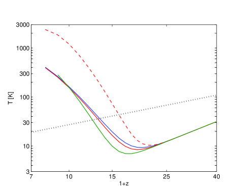
Figure 1: The cosmic mean gas temperature. We show the kinetic gas temperature (averaged over regions that have not yet been reionized) in the cases of molecular cooling halos (blue), atomic cooling halos (red) and massive halos (green). We assume the realistic hard X-ray spectrum of X-ray binaries (solid curves), except that in the atomic cooling case we also compare to a soft power-law spectrum (dashed curve). We show the CMB temperature for comparison (dotted curve). We note that the molecular cooling case includes the effect of the streaming velocity and strong LW feedback, and that the massive halo case has a different star-formation efficiency than the other cases in order to match the optical depth from reionization.

The variation in the model predictions due to different star formation scenarios (i.e., including light halos or not) is only $\Delta z\sim 0.8$, with the redshift of the heating transition being $z=12.3$ and $z=11.5$ for molecular cooling and massive halos, respectively. The differences come from the different halo abundances: the number of massive halos at $z\gtrsim 20$ is small, so heating is initially slow in this case, but it later catches up due to the higher assumed star formation efficiency. In the case of the molecular cooling halos, there is a lot of early structure formation on the corresponding scales, so all the radiative backgrounds ramp up early, but the subsequent time evolution is slower. Thus, the timing of the heating transition is most sensitive to the spectrum of the X-rays (and to their uncertain normalization, as we explored in Fialkov, Barkana & Visbal (2014)).

3.2 Global 21-cm signal

Having cool gas during the first half of reioization has immediate implications for the properties of the observable 21-cm signal emitted at $z=7-15$, as discussed in detail in Fialkov, Barkana & Visbal (2014). However, the slower rise of the gas temperature also affects the predictions for the global 21-cm signal at higher redshifts. In particular, the absorption trough, which is the most prominent feature of the global 21-cm spectrum and whose two steep sides will probably be the easiest to measure, becomes deeper since the gas has more time to cool adiabatically after it thermally decouples from the CMB; the first sources then turn on the 21-cm signal with Ly$\alpha$ emission before they start to warm up the gas.

Our results for the global 21-cm signal are shown in Figure 2 and summarized in Table 1. As in the case of the mean cosmic heating history, the variation among the various cases of star-forming halos (in terms of the depth of the absorption feature which indicates how much the gas cooled before being heated by X-rays) is less significant than the difference between the two X-ray spectra. Specifically, the depth of the absorption trough is increased by $35\%$, or by $\Delta T_{b}\sim 37$ mK, when the realistic case is compared to the soft power-law spectrum for the atomic cooling halos, while the variation due to different star formation histories is only $\Delta T_{b}=8$ mK. Additionally, the emission peak during reionization is reduced by $42\%$ in the case of the hard X-rays. This combination of effects implies that global 21-cm experiments should focus on the Ly$\alpha$ trough rather than on the reionization era. We also note that the redshift of the strongest absorption varies with the halo mass as it depends on the combined timing of the rise of Ly$\alpha$coupling and cosmic heating (see also Furlanetto, Oh & Briggs (2006) and Pritchard & Loeb (2012)).

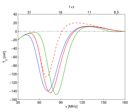
Figure 2: The global 21-cm signal. We show the mean 21-cm brightness temperature $\bar{T}_{b}$ relative to the CMB for the cases of molecular cooling (blue), atomic cooling (red) and massive halos (green). For atomic cooling we also compare to the soft power-law spectrum (dashed curve). Quantitative results from this Figure are summarized in Table 1.

Cooling, SED	Absorption minimum	Heating transition ( $\bar{T}_{b}=0$)	Emission maximum
Atomic, Soft X-rays	$\delta T_{b}=-107$ mK, $\nu=70.0$ MHz	$\nu=91.6$ MHz	$\delta T_{b}=20$ mK, $\nu=112.0$ MHz
Atomic, Hard X-rays	$\delta T_{b}=-144$ mK, $\nu=75.5$ MHz	$\nu=109.3$ MHz	$\delta T_{b}=11.6$ mK, $\nu=129.0$ MHz
Massive, Hard X-rays	$\delta T_{b}=-148$ mK, $\nu=83.5$ MHz	$\nu=114.8$ MHz	$\delta T_{b}=10.8$ mK, $\nu=130.6$ MHz
Molecular, Hard X-rays	$\delta T_{b}=-140$ mK, $\nu=71.5$ MHz	$\nu=107.3$ MHz	$\delta T_{b}=12$ mK, $\nu=128.0$ MHz

Table 1: Characteristic features of the global 21-cm signal.

We note another issue, the small difference between the time at which the mean gas temperature equals the CMB temperature, and the time at which the global mean 21-cm temperature is zero. In linear theory these two times are identical, but in practice non-linearities make the global spectrum vanish a bit later than the moment of equal gas and CMB temperatures. With the old spectrum, this delay is $\Delta z\sim 0.5$ (see also Fialkov et al. (2013)), but the reduced temperature fluctuations in the new spectrum reduce the delay to a much smaller $\Delta z\sim 0.1$. Thus, in what follows, we usually do not consider both times but instead show results only at the later one (when $\bar{T}_{b}=0$, which is closer to being directly observable), and refer to this time as the “heating transition”.

3.3 Fluctuations in the 21-cm signal

The power spectrum of the fluctuations in the 21-cm signal contains much more information than the global signal. Our main focus in this paper is to explore the whole span of this signal, including broad ranges in redshift and scale, and the additional terms from the line-of-sight anisotropy. We begin with Figure 3, which shows the reshift dependence of the power spectrum at various wavenumbers between 0.03 and 1 Mpc^-1, for the four parameter combinations considered here. In addition, we list some of the most interesting numbers that characterize the power spectra in our four cases, for the wavenumbers k = 0.05 Mpc^-1 and k = 0.3 Mpc^-1 in Table 2.

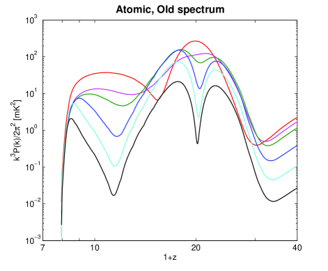
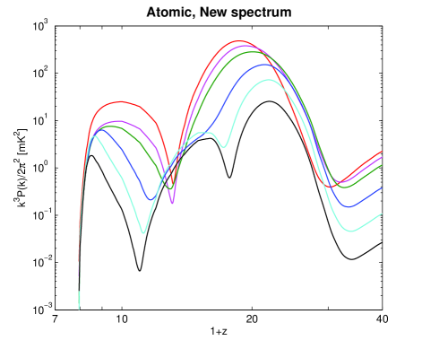
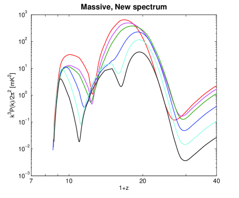
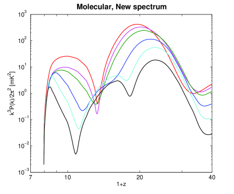
Figure 3: Full power spectrum in mK² units versus redshift at different k: 1 Mpc^-1 (red), 0.5 Mpc^-1 (magenta), 0.3 Mpc^-1 (green), 0.1 Mpc^-1 (blue), 0.05 Mpc^-1 (cyan), and 0.03 Mpc^-1 (black). Top left: atomic cooling with old X-ray SED. Top right: atomic cooling with new SED. Bottom left: massive halos with new SED. Bottom right: molecular halos with new SED.

Cooling, SED, wavenumber	Reion. [mK2]	$z$	Trough [mK2]	$z$	Heating [mK2]	$z$	Ly$\alpha$[mK2]	$z$
Atomic, Soft X-rays, $k$ = 0.3 Mpc-1	13.5	8.6	4.7	11.1	158.5	17.0	97.4	21.6
Atomic, Soft X-rays, $k$ = 0.05 Mpc-1	5.5	7.7	0.1	10.5	74	16.7	43.5	21.9
Atomic, Hard X-rays, $k$ = 0.3 Mpc-1	8.4	7.6	0.36	12.0	-	-	284	19.1
Atomic, Hard X-rays, $k$ = 0.05 Mpc-1	4.7	7.7	0.05	10.2	5.5	14.5	72.6	20.8
Massive, Hard X-rays, $k$ = 0.3 Mpc-1	11.5	9.0	0.55	11.2	-	-	380	17.1
Massive, Hard X-rays, $k$ = 0.05 Mpc-1	9.8	8.4	0.1	10.1	14.0	14.0	116	18.3
Molecular, Hard X-rays, $k$ = 0.3 Mpc-1	7.6	8.3	0.4	12.1	-	-	245	19.8
Molecular, Hard X-rays, $k$ = 0.05 Mpc-1	4.7	7.6	0.05	10.1	4.8	15.1	56	22.1

Table 2: Detailed features of the 21-cm power spectrum shown in Fig. 3. The table shows the values of the power spectrum and the redshift at (from left to right) the reionization peak, the trough around the heating transition, the heating peak, and the Ly$\alpha$peak, for the four considered cases and at two wavenumbers, $k=0.3$ and $k=0.05$ Mpc^-1.

The striking impact of the hard X-rays is that there are no heating fluctuations at the scales where they are expected to be found when soft X-rays heat up the gas. In particular, comparing the two top panels of Fig. 3, which show the two cases of atomic cooling with the soft (left panel) and hard (right panel) X-rays, the peak at $z\sim 15-20$, which appears in the case of soft X-rays at most of the scales presented in the figure ($k<0.5$ Mpc^-1), basically disappears in the case of hard X-rays. Instead of the three peaks (at $k<0.5$ Mpc^-1) which appear due to the inhomogeneous radiative backgrounds (at $z\sim 22$ from the inhomogeneous Ly$\alpha$ background, at $z\sim 17$ due to X-ray heating and at $z\sim 7.5-8$ due to patchy reionization) in the case of the soft X-rays (in agreement with the standard theoretical studies of the 21-cm signal, e.g., Pritchard & Loeb (2008) and Mellema et al. (2013)), with a hard SED there are only two peaks (at $k>0.05$ Mpc^-1) contributed by the fluctuations in the Ly$\alpha$ background and the ionization fraction.

This phenomenon is easy to explain by the fact that the heating is almost uniform in the case of the energetic X-rays emitted by the HMXBs. There are no heating fluctuations on scales smaller than the characteristic mean free path of X-ray photons that contributed to the heating of the gas. On scales larger than the characteristic mean free path of the photons that can be absorbed before the heating fluctuations are saturated, the heating peak is restored (although its height is reduced due to the uniform heating contribution from photons coming from even larger distances). For instance, in the case of the hard SED, the characteristic scale is $k\sim 0.05$ Mpc^-1. Applying the fitting formula of eq. 2 which relates the mean free path to the photon energy, the scale can be translated to the characteristic energy of the X-ray photons which heat the gas, which in this case appears to be $\sim 0.9$ keV. Thus, detecting the heating fluctuation peak and measuring the wavenumber at which it disappears should provide unique information about the characteristic mean free paths, and thus the spectral energy distribution, of the photons that heat the gas. In case of the soft spectrum, a heating fluctuation peak should be found on much smaller scales, but it disappears at $k\sim 0.5$ Mpc^-1 and above, which corresponds to a characteristic X-ray energy of $\sim 0.4$ keV (note that the soft spectrum implemented here has a cutoff at 0.2 keV). Note that some 21-cm signatures of heating sources with different X-ray spectra have also been discussed by Pacucci et al. (2014).

In addition, in the cases with the hard X-rays, the trough seen in the power spectra at $z\sim 10-12$ is deeper than in the case of the soft X-rays by a scale-dependent factor. For instance, Table 2 shows that at k = 0.3 Mpc^-1 the spectrum goes as low as 0.36 mK² instead of 4.7 mK², which means (after applying a square root) weaker fluctuations by a factor of four. This feature was extensively discussed in Fialkov, Barkana & Visbal (2014).

The same characteristic behaviors listed above are seen in the cases of the massive halos and the molecular cooling halos, shown in the bottom row of Fig. 3. The only major difference between the various star formation scenarios here, as in the case of the global spectrum, is the earlier, but slower, evolution in the case of molecular cooling halos, resulting also in a slight shift of the Ly$\alpha$ peak toward higher redshifts, and (on the other hand) the later but more intense rise of the signal in the case of the massive halos.

In Fig. 4 we show a different cut of the parameter space: the total 21-cm power spectrum versus wavenumber, at each of several key redshifts: redshift during reionization at which the power spectrum magnitude at k = 0.1 Mpc^-1 reaches its maximum (referred to as the reionization peak), the midpoint of reionization (i.e., $x_{i}=0.5$), the moment when $x_{i}=0.25$, the redshift at which heating fluctuations peak (in the case of the old SED) or the redshift of the heating transition (in the case of the new SED), the minimum of the global brightness temperature, the redshift at which fluctuations from Ly$\alpha$ peak, and a high redshift (here $z=30$) at which the 21-cm fluctuations are dominated by fluctuations in density, although small Ly$\alpha$ fluctuations are already present. Comparing the two cases of atomic cooling again, we see that shape of the power spectrum is most sensitive to the type of the SED at the early stages of reionization (here shown for $x_{i}=0.25$) and during heating, where the key feature is a peak of heating fluctuations (in the case of the old SED) or a minimum around the heating transition (in the case of the new SED). Comparing the various halo masses (all with the new SED), the more massive halos tend to produce a higher signal due to the higher halo bias (i.e., stronger clustering), though other factors are also critical (such as the faster rise of the cosmic star formation rate for more massive halos, which affects heating and Ly$\alpha$ coupling). In general, the exact shape of the power spectrum has a complex dependence on the various parameters.

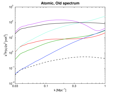
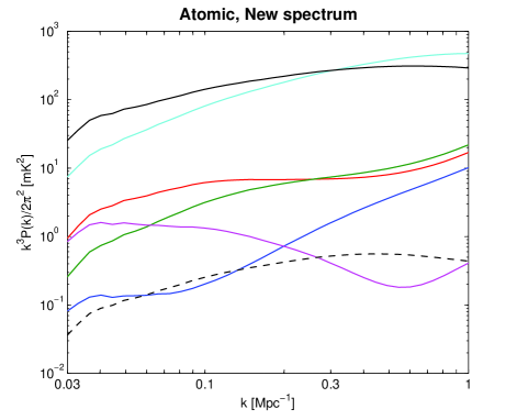
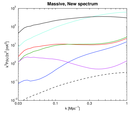
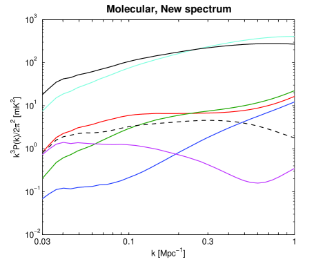
Figure 4: Power spectrum in mK² units versus wavenumber $k$ in Mpc^-1, at several important redshifts (in order from low to high): that of the reionization peak at $k=0.1$ Mpc^-1 (red solid line), the midpoint of reionization (i.e., $x_{i}=0.5$) (green solid line), $x_{i}=0.25$ (blue solid line), the peak of the heating fluctuations (in the case of the old SED) or of the heating transition (in the case of the new SED) (magenta solid line), the minimum of the global $\bar{T}_{b}$ (cyan solid line), peak of fluctuations from Ly$\alpha$ (black solid line), and $z=30$ (black dashed line). Top left: atomic cooling with old SED, at $z=8$ (corresponds to $x_{i}=0.66$, red), 8.7 (green), 10.7 (blue), 16.8 (magenta), 19 (cyan), 22 (black solid), 30 (black dashed). Top right: atomic cooling with new SED, at $z=8$ ($x_{i}=0.66$, red), 8.7 (green), 10.7 (blue), 12.1 (magenta), 18 (cyan), 20.4, 30 (black dashed). Bottom left: massive halos with new SED, at $z=8.6$ ($x_{i}=0.6$, red), 8.9 (green), 10.3 (blue), 11.3 (magenta), 16 (cyan), 18.1 (black solid), 30 (black dashed). Bottom right: molecular cooling halos with new SED, at $z=7.9$ ($x_{i}=0.67$, red), 8.6 (green), 10.6 (blue), 12.3 (magenta), 19 (cyan), 21.2 (black solid; close to the Ly$\alpha$ peak at 21.7), 30 (black dashed).

As mentioned above, it may be useful to analyze the angular dependence of the power spectrum in order to learn from the same measurement about both astrophysics and cosmology (Barkana & Loeb, 2005a; Pritchard & Loeb, 2008). As was shown by Barkana & Loeb (2005a) (and as we mentioned in sec. 2), the unique three-dimensional properties of 21 cm measurements permit a separation of the total power spectrum to components according to their angular dependence: $P(k)=P_{\rm iso}+P_{X}+P_{\delta}$. Even if in practice this separation cannot be achieved cleanly (we plan to further study this issue), the additional information from the angular dependence will provide added astrophysical information and further tests of the predictions of simulated models. In Fig. 5 we show the redshift dependence of each component (also including the total power spectrum) at a specific wavenumber $k=0.1$ Mpc^-1 for the four histories under consideration. The dominant contribution to the total power comes from the isotropic component, i.e., astrophysical sources, while the contribution of the density two-point function $P_{\delta}$ is generally smaller by between a factor of a few and 100. On the other hand, $P_{X}$, which is the cross-correlation between the isotropic part and the density fluctuations, is boosted with respect to $P_{\delta}$ and can be used to further confirm and constrain the astrophysical information.

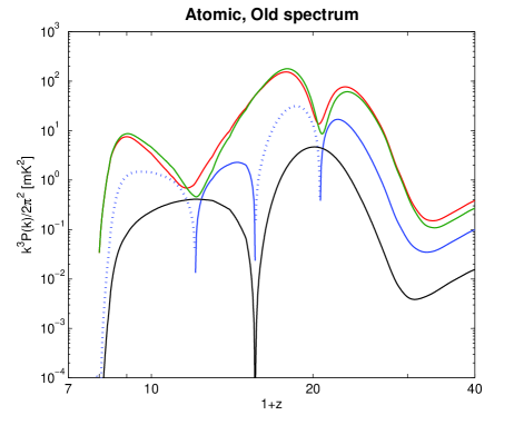
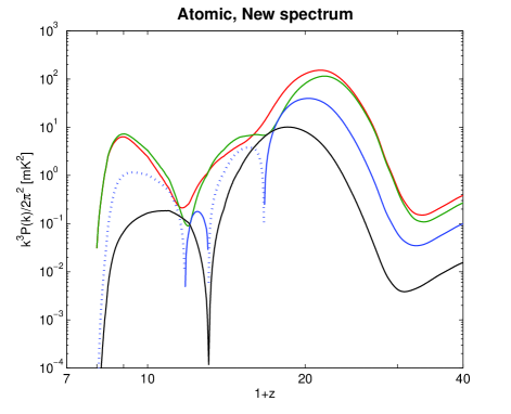
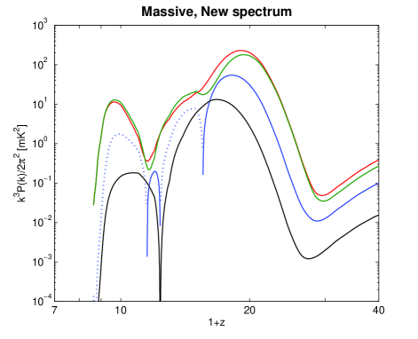
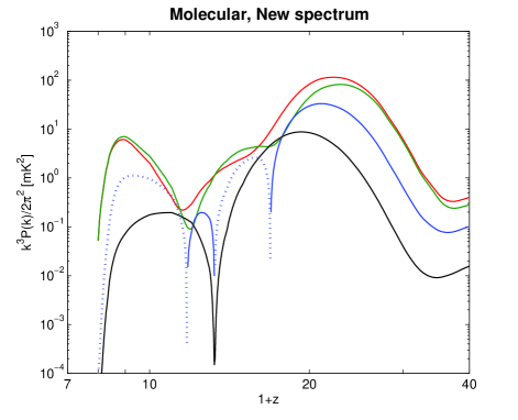
Figure 5: Power spectrum in mK² units at $k=0.1$ Mpc^-1 versus redshift. We show the full spectrum (red), the isotropic contribution $P_{\rm iso}$ (green), $P_{\delta}$ (black), and $P_{X}$ where it is positive (solid blue) or $-P_{X}$ where it is negative (dotted blue). Top left: atomic cooling with old SED. Top right: atomic cooling with new SED. Bottom left: massive halos with new SED. Bottom right: molecular cooling halos with new SED.

An important qualitative feature is that $P_{X}$ is positive or negative at various times, and its sign changes are correlated with changes in the shape of other components (such as $P_{\rm iso}$), since they indicate the dominance of various fluctuation sources. To analyze this, first note that through the line-of-sight gradient term, a positive density fluctuation in a given pixel (which yields an infall velocity pattern that opposes the Hubble expansion and increases the total 21-cm optical depth) always tends to increase the magnitude of $T_{b}$ in the pixel (regardless of its sign). Now, the 21-cm effect of ionization fluctuations is anti-correlated (since positive density fluctuations implies more ionization, fewer hydrogen atoms, and thus a lowered 21-cm optical depth). This is why $P_{X}$ is negative at the lowest redshifts, where ionization fluctuations dominate the 21-cm signal (e.g., at $k=0.1$ Mpc^-1 as shown in the figure). In this redshift region, $P_{\rm iso}$ (as well as the total 21-cm $P(k)$) rises with time towards the reionization peak, before falling again as reionization is completed. Now, when the 21-cm fluctuations are dominated by heating fluctuations, higher density implies stronger heating, and higher $T_{K}$ implies higher $T_{b}$; this is the same as increasing $|T_{b}|$ if $T_{b}>0$, but it is the opposite if $T_{b}<0$. Thus, $P_{X}$ during this redshift interval is positive after the heating transition and negative before it. In particular, the old spectrum case shows a substantially extended redshift range with positive $P_{X}$ since the heating transition occurs much earlier in this case. Note that while the heating peak (for the soft spectrum) or minimum (for the hard spectrum) does not occur right at the heating transition (except on small scales for the hard spectrum), there is a predicted transition from negative to positive $P_{X}$ very close to the time when $\bar{T}_{b}=0$. At higher redshifts, when Ly$\alpha$ fluctuations dominate the 21-cm fluctuations, $P_{X}$ is positive since higher density implies a higher Ly$\alpha$ intensity and thus a higher magnitude of $T_{b}$. At the highest redshifts, $P_{X}$ remains positive as the 21-cm fluctuations become dominated by the direct effect of density fluctuations along with the associated adiabatic heating.

Looking more broadly at the shape of the curves with redshift, we again see that in going from the soft to the hard spectrum, the peak from heating fluctuations disappears from the signals affected by star formation, i.e., the total power spectrum, the isotropic part and the cross-term (in $P_{X}$ there are still two peaks during the heating era, due to the sign changes explained above, though they are at substantially lowered fluctuation levels); whereas the impact on $P_{\delta}$ is only via the global $\delta T_{b}$ history. We again note that here $P_{\delta}$ is given in mK² units, i.e., it has been multiplied by the square of $\bar{T}_{b}$, which for example drives the power spectrum to zero at the heating transition when the global spectrum vanishes.

In order to show the various power spectrum components over a range of wavenumbers, at least for one case (atomic cooling with hard X-rays), in Fig. 6 we show the various contributions versus $k$ at several redshifts which represent different epochs of cosmic history. This figure shows that the redshifts at which $P_{X}$ changes sign depend on $k$, or equivalently, at a given redshift $P_{X}$ may have a different sign at different $k$. In particular, at the heating transition, the fluctuations on most scales are dominated by temperature fluctuations (for which $P_{X}>0$ at this time), but at $z=12$ ionization (with its negative associated $P_{X}$) already dominates small scales ($k>0.6$ Mpc^-1). As reionization progresses, ionization fluctuations come to dominate larger and larger scales, until they dominate the full range of probed scales. At each redshift (from early to late reionization), the switch in the dominant source of fluctuations at a particular $k$ is marked both by a switch in the sign of $P_{X}$ and in the shape of $P_{\rm iso}$ (as well as the total 21-cm power spectrum).

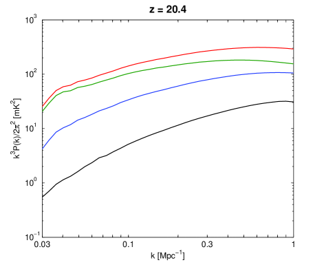
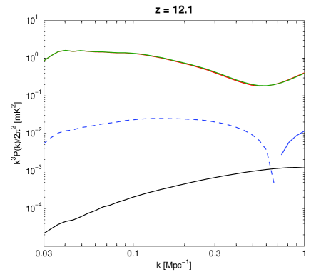
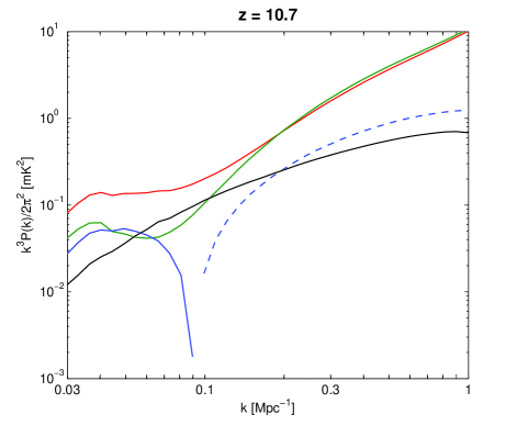
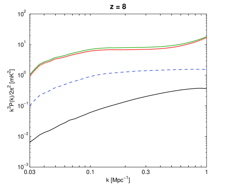
Figure 6: Power spectra (in mK² units) of various components for a single parameter case (atomic cooling with the new spectrum) versus wavenumber, shown at various redshifts. We show the full spectrum (red), the isotropic contribution (green), $P_{\delta}$ (black), the positive $P_{X}$ (solid blue) or minus the negative $P_{X}$ (dashed blue). Top left: $z=20.4$ (the peak of fluctuations from Ly$\alpha$). Top right: $z=12.1$ (heating transition). Bottom left: $z=10.7$ (redshift that corresponds to $x_{i}=0.25$). Bottom right: $z=8$ (reionization peak for $k=0.1$ Mpc^-1).

Finally, for visual comparison and physical intuition we show some snapshots of the gas temperature and the 21-cm brightness temperature (Figure 7). We take two redshifts at which the effect of the different SEDs is apparent, choosing 8.7 (the midpoint of reionization for $\tau=0.075$) and 12.1 (a redshift early in reionization ($x_{i}=0.14$), which marks the heating transition for the hard spectrum). We compare the soft and hard X-ray spectra for the case of atomic cooling. In this comparison, both cases have the same underlying distribution of star formation at a given redshift, so they have the same ionized patches and a similar distribution pattern of gas temperature and of 21-cm temperature. However, the difference is visually striking, in that the maps for the hard spectrum are strongly suppressed both in terms of the absolute values and in the relative size of the fluctuations.

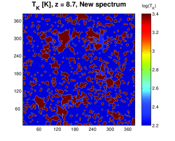
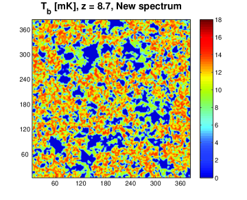
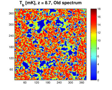
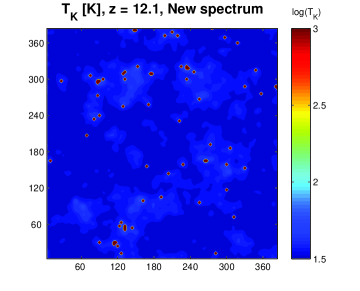
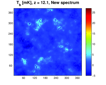
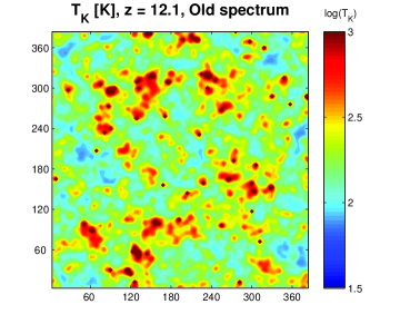
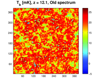
Figure 7: Two-dimensional slices of the logarithm of the gas temperature $T_{K}$ in Kelvin (left column) and of the 21-cm brightness temperature (relative to the CMB) $T_{b}$ in mK (right column), for the two cases of atomic cooling halos. Note that the two cases have identical reionization histories, with fully-ionized pixels shown with the color corresponding to the hottest $T_{K}$ (on the left) and to $T_{b}=0$ (on the right). From top to bottom: hard X-rays at $z=8.7$, which gives ranges $T_{K}=165-210$ K and $T_{b}=2.1-14.5$ mK; soft X-rays at $z=8.7$, with ranges $T_{K}=703-2946$ K and $T_{b}=2.4-16.8$ mK; hard X-rays at $z=12.1$, with ranges $T_{K}=30.6-56.5$ K and $T_{b}=-4.8-8.4$ mK; and soft X-rays at $z=12.1$, with ranges $T_{K}=75.9-1742$ K and $T_{b}=0.8-27.4$ mK. Note that $z=12.1$ corresponds to $x_{i}=0.14$ and to the heating transition for the hard spectrum, while $z=8.7$ corresponds to $x_{i}=0.5$. At each redshift, we use a common scale for the two spectra, for ease of comparison.

4 Summary and Discussion

The impact of high-mass X-ray binaries on early cosmic heating and on the global 21-cm signal has been previously discussed in the literature (§ 1). However, the case in which X-rays emitted by high-redshift sources are inefficient in heating up the cosmic gas was considered very extreme, and thus not too interesting. In our recent paper (Fialkov et al., 2014) we challenged this belief, showing that high-redshift X-ray sources are likely inefficient in heating up the Universe and producing fluctuations in the gas temperature. While the heating mechanisms at high redshifts are still rather unconstrained, in our work we assumed that the dominant X-ray sources at high redshifts are HMXBs with hard X-ray spectra. This assumption was based on the results of the population synthesis simulation by Fragos et al. (2013), calibrated to low-redshift observations and evolved with redshift accounting for the effect of the evolution of metallicity. Based on current knowledge, the contribution of HMXBs to heating likely wins over soft X-ray emission from hot gas at high redshifts, given the fact that (1) today the total X-ray energy is dominated by X-ray binaries over hot gas; (2) both theory and observations suggest that the contribution of X-ray binaries increases by an order of magnitude at the low metallicities expected at high redshift; and (3) although it is true that hard X-rays interact less with the gas, a significant fraction of their energy is still absorbed after being redshifted, and thus, the fluctuations from soft X-rays are reduced if hard X-rays provide a large, uniform background contribution. In this paper, in addition to our main ”New spectrum” case which we consider most likely, we also considered the much softer ”Old spectrum”. Together these two cases reasonably bracket the range of possibilities. We believe it is important to consider a range of X-ray spectra when making predictions for future 21-cm surveys, since in the end only the observations will determine the nature of high-redshift heating sources.

Here we discussed for the first time the effect of hard X-rays on the history of fluctuations in the 21-cm signal during the entire range of redshifts $z=7-40$, from the epoch of primordial star formation to the end of reionization (expanding on Fialkov, Barkana & Visbal (2014)). This is a particularly timely as it shows that the signal, which will likely be observed in near future, may be significantly different than predicted with the previously-assumed soft X-ray spectrum. The effect of the hard spectra of HMXBs, which were likely the main source of X-rays in the early universe (Fragos et al., 2013), was not considered in the majority of previous works.

The main consequences of the heating by HMXBs with a hard spectrum that peaks at $\sim 3$ keV are the following:

1. A dramatic difference in comparison with soft X-rays is that the universe is heated more slowly due to the fact that the hard X-rays have longer mean free paths and thus are less efficiently absorbed by the cosmic gas. Specifically, the heating transition is delayed by a $\Delta z\sim 3$, whereas the variation due to the various star-formation scenarios considered here is only $\Delta z\sim 0.8$.

2. Since the gas cools adiabatically for much longer, it produces a stronger 21-cm absorption signal early on. On the other hand, during reionization the gas is only moderately warm, and its emission signal is suppressed. This combination implies that global 21-cm experiments should focus on $z\sim 20$ rather than on the reionization era.

3. The heating is also much more uniform. As a result, the heating fluctuation peak, expected to be found in scenarios with the soft X-rays, disappears at intermediate scales of $k>0.05$ Mpc^-1. The wavenumbers at which the heating peak is detected in observations should tell us about the characteristic mean free path and spectrum of the emitted photons, thus giving key clues as to the character of the sources that heated the primordial Universe. In addition, the minimum around $z\sim 10-12$ which separates the heating and ionization domains becomes much deeper. The fluctuations are weaker by a factor of $2-13$ (depending on the scale) at the minimum.

The line-of-sight anisotropy makes the analysis of 21-cm fluctuations much richer, as it in principle allows for three power spectra to be extracted at each redshift, the isotropic term $P_{\rm iso}$, its cross-correlation with density $P_{X}$, and the density power spectrum (times a factor of $\bar{T}_{b}^{2}$) $P_{\delta}$. The main conclusions regarding these components of the power spectra are:

1. The isotropic term $P_{\rm iso}$ is the leading contribution to the total power spectrum at all scales and all the considered epochs. $P_{X}$ is sometimes comparable in magnitude but typically smaller by a factor of a few. $P_{\delta}$ is the smallest and thus will be the hardest to measure.

2. $P_{X}$ is particularly interesting since it changes sign in a way that encodes information on the various sources of 21-cm fluctuations. For example, it changes sign at the heating transition, a moment in which (more generally) the anisotropy of the power spectrum drops to near zero. Also, $P_{X}$ is negative when ionization fluctuations dominate during reionization, and positive at the highest redshifts.

3. The dominance of various fluctuation sources depends on wavenumber, and can be probed at each redshift from the sign of $P_{X}$ at various $k$ as well as corresponding slope changes in $P_{\rm iso}$.

Our predictions affect the expectations for the 21-cm signal in the range that is observable in the near future. The reionization peak should be within the sensitivity of present day observatories (such as LOFAR and the MWA). These experiments may also be able to find signs of the trough at $z\sim 10-15$, but for hard X-rays the low level of these fluctuations may require the SKA for detection. At higher redshifts ($z=15-20$), the expected SKA sensitivity to the power spectrum ($k^{3}P(k)/2\pi^{2}$) of around a mK² on large scales (McQuinn et al., 2006) should allow for a detailed measurement of the 21-cm power spectrum; in particular, a heating peak should be detected or ruled out. The strong peak of Ly$\alpha$ fluctuations at $z\sim 20$ (for any scenario of star formation considered here) should also be detectable, since the sensitivity of the SKA is expected to be of order 10 mK² at $z\sim 20$. At several of these redshift ranges (particularly the peaks), the SKA should have sufficient extra sensitivity to probe the anisotropy of the 21-cm power spectrum and get a useful measurement of $P_{X}$. At the same time, global 21-cm experiments can give complementary information, such as verifying late heating by measuring a deep minimum in the global signal below $-140$ mK.

5 Acknowledgments

A.F. was supported by the LabEx ENS-ICFP: ANR-10-LABX-0010/ANR-10-IDEX- 0001-02 PSL and NSF grant AST-1312034. R.B. acknowledges Israel Science Foundation grant 823/09 and the Ministry of Science and Technology, Israel.

References

- Abel, Bryan & Norman (2002) Abel, T., Bryan, G. L. Norman, M. L., 2002, Science, 295, 93
- Ade et al. (2013) Ade, P. A. R. et al., 2013, arXiv:1303.5076
- Barkana & Loeb (2005a) Barkana, R. & Loeb, A., 2005, ApJ, 624, 65
- Barkana & Loeb (2005b) Barkana, R. & Loeb, A., 2005, ApJ, 626, 1
- Baek et al. (2010) Baek, S., Semelin, B., Di Matteo, P., Revaz, Y. & Combes, F., 2010, A& A, 523, 4
- Bennett et al. (2013) Bennett, C. L., et al., 2013, ApJS, 208, 20
- Bharadwaj & Ali (2004) Bharadwaj, S., & Ali, S. S., 2004, MNRAS, 352, 142
- Bowman et al. (2013) Bowman, J. D. et al., 2013, PASA, 30, 31.
- Brandenberger et al. (2010) Branderberger, R. H., Danos, R. J., Hernandez, O. F. & Holder, G. P., 2010, JCAP, 12, 028
- Bromm (2013) Bromm, V., 2013, RPP, 76, 2901
- Burns et al. (2012) Burns, J. O., Lazio, J., Bale, S., Bowman, J., Bradley, R. et al., 2012, AdSpR, 49 433.
- Ciardi, Salvaterra & Di Matteo (2013) Ciardi, B., Salvaterra, R. & Di Matteo, T., 2010, MNRAS, 401, 2653
- Dalal, Pen & Seljak (2010) Dalal, N., Pen, U.L. & Seljak, U., 2010, JCAP, 11, 7.
- Ellingson et al. (2013) Ellingson, S. W., Craig, J., Dowell, J., Taylor, G. B., Helmboldt, J. F., 2013 arXiv:1307.0697.
- Fialkov et al. (2012) Fialkov, A., Barkana, R., Tseliakhovich, D., Hirata, C. M., 2012, MNRAS, 424, 1335
- Fialkov et al. (2013) Fialkov, A., Barkana, R., Visbal, E., Tseliakhovich, D. & Hirata, C. M., 2013, MNRAS, 432, 2909s
- Fialkov et al. (2014) Fialkov, A., Barkana, R., Pinhas, A., Visbal, E., 2014, MNRAS, 437, 36 432, 2909
- Fialkov, Barkana & Visbal (2014) Fialkov, A., Barkana, R. & Visbal, E., 2014, Nature, 506, 197
- Fragos et al. (2013) Fragos, T., Lehmer, B. D., Naoz, S., Zezas, A. & Basu-Zych, A., 2013, ApJ, 776, 31
- Furlanetto (2006) Furlanetto, S. R., 2006, MNRAS, 371, 867
- Furlanetto & Loeb (2004) Furlanetto, S. R., & Loeb, A. 2004, ApJ, 611, 642
- Furlanetto, Oh & Briggs (2006) Furlanetto, S. R., Oh, S. P. Briggs, F. H., 2006, PhR, 433, 181
- Greif et al. (2011) Greif, T. H., White, S. D. M., Klessen, R. S. & Springel, V., 2011, ApJ, 736, 147.
- van Haarlem (2013) van Haarlem, M. P. et al., 2013, A& A, 556, 2.
- Haiman, Thoul & Loeb (1996) Haiman, Z., Thoul, A. A. Loeb, A., 1996, ApJ, 464, 523
- Haiman, Abel & Rees (2000) Haiman, Z., Abel, T. Rees, M. J., 2000, ApJ, 534, 11
- Iliev et al. (2014) Iliev, I. T. et al., 2014, MNRAS, 439, 725.
- Machacek, Bryan & Abel (2010) Machacek, M. E., Bryan, G. L. Abel, T., 2001, ApJ, 548, 509
- Madau, Meiksin & Rees (1997) Madau, P., Meiksin, A. & Rees, M. J., 1997, ApJ, 475, 429
- Majumdar et al. (2013) Majumdar, S., Bharadwaj, S., & Choudhury, T. R. 2013, MNRAS, 434, 1978
- Mao et al. (2012) Mao, Y., Shapiro, P. R., Mellema, G., et al. 2012, MNRAS, 422, 926
- McQuinn et al. (2006) McQuinn, M., Zahn, O., Zaldarriaga, M., Hernquist, L. & Furlanetto, S. R., 2006, ApJ, 653, 815
- McQuinn & O’Leary (2013) McQuinn, M. & O’Leary, R. M., 2012, ApJ, 760, 3
- Mellema et al. (2013) Mellema G. et al., 2013, ExA, 36, 235
- Mesinger, Furlanetto & Cen (2011) Mesinger, A., Furlanetto, S. Cen, R., 2011, MNRAS, 411, 955
- Mineo, Gilfanov & Sunyaev (2012) Mineo, S., Gilfanov, M. & Sunyaev, R., 2012, MNRAS, 426, 1870
- Mirabel et al. (2011) Mirabel, I. F., Dijkstra, M., Laurent, P., Loeb, A. & Pritchard, J. R., 2011, A&A, 528, 149
- Naoz & Barkana (2008) Naoz, S., Barkana, R., 2008, MNRAS, 385, L63
- Naoz, Noter & Barkana (2006) Naoz, S., Noter, S. & Barkana, R., 2006, MNRAS, 373, L98
- Naoz et al. (2013) Naoz, S., Yoshida, N., Gnedin, N. Y., 2013, ApJ, 763, 27
- O’Shea & Norman (2000) O’Shea, B. W. Norman, M. L., 2008, ApJ, 673, 14
- Oh (2001) Oh, S. P., 2001, ApJ, 553, 499
- Paciga et al. (2013) Paciga, G., Albert, J. G., Bandura, K. et al., 2013, MNRAS, 433, 639
- Pacucci et al. (2014) Pacucci, F., Mesinger, A., Mineo, S., & Ferrara, A. 2014, arXiv:1403.6125
- Parsons et al. (2010) Parsons, A. R., Backer, D. C., Foster, G. S., Wright, M. C. H., Bradley, R. F. et al., 2010, AJ, 139, 1468.
- Patil et al. (2014) Patil, A. H., et al. 2014, arXiv:1401.4172
- Pober et al. (2014) Pober, J. C., et al. 2014, ApJ, 782, 66
- Pritchard & Loeb (2008) Pritchard, J. R., A. Loeb, A., 2008, PRD, 78, 3511
- Pritchard & Loeb (2012) Pritchard, J. R., A. Loeb, A., 2012, PRD, 75, 6901
- Rephaeli (1995) Rephaeli, Y., Gruber D. & Persic M., 1995, AA, 300, 91.
- Ricotti, Ostriker & Mack (2008) Ricotti, M., Ostriker J. P. & Mack K. J., 2008, ApJ, 680, 829.
- Schroeder, Mesinger, & Haiman (2013) Schroeder, J., Mesinger, A., Haiman, Z., 2013, MNRAS, 428, 3058
- Shapiro et al. (2013) Shapiro, P. R., Mao, Y., Iliev, I. T., et al. 2013, Physical Review Letters, 110, 151301
- Stacy, Bromm & Loeb (2011) Stacy, A., Bromm, V. & Loeb, A., 2011, MNRAS, 730, 1.
- Tanaka, Perna & Haiman (2012) Tanaka, T., Perna, R. & Haiman, Z., 2012, MNRAS, 425, 2974
- Tegmark et al. (1997) Tegmark, M., Silk, J., Rees, M., Blanchard, A., Abel, T., Palla, F., 1997, ApJ, 474, 1
- Tseliakhovich & Hirata (2010) Tseliakhovich, D. Hirata, C. M., 2010, PRD, 82, 3520
- Tseliakhovich, Barkana & Hirata (2011) Tseliakhovich D., Barkana R., Hirata C. M., 2011, MNRAS, 418, 906
- Valdes et al. (2013) Valdes, M., Evoli, C., Mesinger, A., Ferrara, A. & Yoshida, N., 2013, MNRAS, 429, 1705.
- Van der Hulst (1945) Van de Hulst, H. C., 1945, NTN, 11, 201
- Visbal et al. (2012) Visbal, E., Barkana, R., Fialkov, A., Tseliakhovich, D. Hirata, C. M., 2012, Nature, 487, 70
- Visbal et al. (2014) Visbal, E., Haiman, Z., Terrazas, B., Bryan, G. L., & Barkana, R., 2014, arXiv:1402.0882.
- Wise & Abel (2000) Wise, J. H. Abel, T., 2007, ApJ, 671, 1559
- Zawada et al. (2014) Zawada, K., Semelin, B., Vonlanthen, P., Baek, S. & Revaz, Y., 2014, MNRAS, tmp, 262