Impromptu Deployment of Wireless Relay Networks: Experiences Along a Forest Trail

Abstract

We are motivated by the problem of impromptu or as-you-go deployment of wireless sensor networks. As an application example, a person, starting from a sink node, walks along a forest trail, makes link quality measurements (with the previously placed nodes) at equally spaced locations, and deploys relays at some of these locations, so as to connect a sensor placed at some a priori unknown point on the trail with the sink node. In this paper, we report our experimental experiences with some as-you-go deployment algorithms. Two algorithms are based on Markov decision process (MDP) formulations; these require a radio propagation model. We also study purely measurement based strategies: one heuristic that is motivated by our MDP formulations, one asymptotically optimal learning algorithm, and one inspired by a popular heuristic. We extract a statistical model of the propagation along a forest trail from raw measurement data, implement the algorithms experimentally in the forest, and compare them. The results provide useful insights regarding the choice of the deployment algorithm and its parameters, and also demonstrate the necessity of a proper theoretical formulation.

I Introduction

Our work in this paper is motivated by the need for as-you-go deployment of wireless relay networks over large terrains, such as forest trails, where planned deployment would be time-consuming and difficult. As-you-go deployment is the only choice when the network is temporary and needs to be quickly redeployed, or when the deployment needs to be stealthy.

In this paper, we are concerned with an experimental study of the problem of deploying wireless relay nodes as a deployment agent walks along a forest trail, in order to connect a sink at the start of the trail to a sensor that would need to be deployed at an a priori unknown point. The sensor could be an animal activity detector based on passive infra-red (PIR) sensors, or even a “camera trap,” that has to be placed near a watering hole that is known to exist somewhere just off the trail. Figure 1 depicts the abstraction of the problem along a line. The sink has a “backhaul” communication link to a control center.

In planned deployment, we need to place relay nodes at all potential locations (see Figure 1 for a simple depiction) and measure the qualities of all possible (solid and dotted) links (between all pairs of potential locations; see Figure 1) in order to decide where to place the relays. This would yield a global optimal solution, but with huge time and effort. With as-you-go deployment, the next relay placement locations depend on the radio link qualities to the previously placed nodes; link qualities and the location of the sensor node are discovered as the agent walks along the trail. Such an approach requires fewer measurements compared to planned deployment, but is suboptimal. In this paper, we report the results of our experimentation with some as-you-go deployment algorithms (taken from our prior work [1] which is an extension of [2], one heuristic adapted from the literature, and one proposed in this paper) on a forest trail in the campus of Indian Institute of Science, Bangalore.

Figure 1: Two wireless relays (filled dots) deployed along a line to connect a source to a sink by a multihop path. The unfilled dots show other potential relay placement locations, the thin dashed lines indicate all the potential links between the potential placement locations, and the solid lines with arrowheads indicate the links actually used in the deployed network.

Related Work: Souryal et al. [3] provide a deployment protocol employing real-time assessment of wireless link quality. As the agent walks away from the sink, signal quality measurements are made with already placed nodes, and a threshold-based algorithm determines when it is opportune to place another relay. One of the algorithms that we include in our experimental study is a simple adaptation of the algorithm reported in [3]. Liu et al. [4] proposed the Breadcrumb System to aid fire-fighters inside a building. The system drops tiny radio relays (“breadcrumbs”) as a firefighter walks; the impromptu wireless network so created is used to send the firefighter’s physiological parameters back to the control truck outside the building. See [5] and [6] for other approaches.

However, there has been little effort to rigorously formulate the problem in order to derive optimal policies which are insightful and which can provide improved performance compared to reasonable heuristics. Recently, Sinha et al. [7] have provided a Markov decision process (MDP) formulation for establishing a multi-hop network between a destination and an unknown source location by placing relay nodes along a random lattice path. They assume a given deterministic mapping between power and wireless link length; this is achieved by employing a very conservative fade margin to take care of the joint effects of shadowing and fast fading, thereby to determine the transmit power required to maintain the link quality over links of a given length. We considered the possibility of link outage, and brought in the idea of measurement based optimal impromptu placement, first in [2] and next in the extended version [1].

II System Model and Deployment Setting

Deployment is done by a single agent (in one “pass”) along a line discretized in steps of length $\delta$ (e.g., $20$ meters), and these discrete locations are the potential relay locations.

II-A Channel Model

The received power (for the $k$-th packet) for a link of length $r$ is given by $P_{rcv,k}=P_{T}c(\frac{r}{r_{0}})^{-\eta}H_{k}W$, where $P_{T}$ is the transmit power, $c$ corresponds to the path-loss at the reference distance $r_{0}$, $\eta$ is the path-loss exponent, $H_{k}$ denotes the fading random variable (varying with time for a link) for the $k$-th packet, and $W$ denotes the shadowing random variable (constant for a link but varies over different links). $W$ is modeled as a log-normal random variable; $W=10^{\frac{\nu}{10}}$, $\nu\sim\mathcal{N}(0,\sigma^{2})$. The mean received power (averaged over fading) in a link with shadowing realization $w$ is $\overline{P}_{rcv}=P_{T}c(\frac{r}{r_{0}})^{-\eta}w\mathbb{E}(H)$. We assume that the shadowing random variables at any two different links are independent; this holds if $\delta$ is greater than the shadowing decorrelation distance (see Section V).

A link is considered to be in outage if the received signal power (RSSI) drops (due to fading) below a value $P_{rcv-min}$. For packet size of $140$ bytes and for TelosB motes, the packet error rate (PER) is less than $2\%$ at RSSI $-88$ dBm, and increases rapidly as RSSI decreases further (see [8]). Hence, for TelosB motes, we choose $P_{rcv-min}=-88$ dBm.

The transmit power of each node can be chosen from a discrete set, $\mathcal{S}$. If the fading statistics are known, then the outage probability is $P_{out}(r,\gamma,w):=\mathbb{P}(\gamma c(\frac{r}{r_{0}})^{-\eta}Hw\leq P_{rcv-min})$ for a link of length $r$ and shadowing realization $w$ ($w$ is unknown) at a particular transmit power level $\gamma$. We can measure $P_{out}(r,\gamma,w)$ for a link with length $r$, transmit power $\gamma$ and shadowing realization $w$ by sending a large number of packets over multiple coherence times and then obtaining the fraction of packets whose RSSI value is below $P_{rcv-min}$.

II-B Deployment Process

We consider two deployment approaches: (i) limited exploration based, and (ii) pure as-you-go. We explain these alternatives with reference to Figure 2. The agent walks away from the sink (from left to right in the figure), evaluating whether to place relays at the potential placement points that are at multiples of the step length $\delta$. Suppose a relay has been placed at the position marked by the $\mathsf{x}$ in Figure 2. Let us denote by $w_{r}$, the realization of shadowing from the location which is $r$ steps ahead of the placed relay, to this relay. For deployment with limited exploration, as the deployment agent walks along the line, after placing a node, he measures the outage probabilities $P_{out}(r,\gamma,w_{r})$ to the previous node from locations $r\in\{1,\cdots,B\}$, at each power level $\gamma\in\mathcal{S}$ (see Figure 2; $\mathcal{S}$ is the finite set of transmit power levels that a node can use). Then he places the relay at one of the locations $1,2,\cdots,B$, sets it to operate at a certain transmit power (both decisions being made by the algorithm). Recursively, this relay then becomes $\mathsf{x}$, the deployment agent moves forward and applies the same procedure to deploy additional relays. If the source location is encountered within $B$ steps from the previous node (i.e., the "current $\mathsf{x}$"), then the source is placed.

With pure as-you-go (no exploration), the agent measures $\{P_{out}(r,\gamma,w_{r})\}_{\gamma\in\mathcal{S}}$ when he is $r$ steps away from the previous relay, and at each step (after making the measurement) the algorithm decides whether to place a relay there or whether to advise the agent to move on without placing. In this process, if he has walked $B$ steps away from the previous relay, or if he encounters the source location, then he must place a node.

II-C Traffic Model

The formulations from which the algorithms are derived in [1] assume a very light traffic model, the assumption being that there is only one packet in the network at a time; we call this the “lone packet model.” Thus, the formulations assume that there are no simultaneous transmissions to cause interference. It is a good approximation for sensor networks that just carry an occasional alarm packet, or low duty-cycle measurement packets. It has been shown in [9] that, under a CSMA MAC, in order to achieve a target delivery probability under any packet arrival rate, it is necessary to achieve the target delivery probability under the lone packet traffic model.

Figure 2: The agent places a relay (shown by an “$\mathsf{x}$”) and makes measurements to obtain the outage probabilities $\{p_{out}(r,\gamma,w_{r})\}$, $r\in\{1,2,3\}$, $\gamma\in\mathcal{S}$, from successive potential locations. With $B=3$, measurements from $3$ successive locations are made before making a placement decision.

II-D Network Cost and Optimality Objective

Under lone packet traffic, the cost of a deployed network is the sum of certain hop costs. In case all the nodes have wake-on radios, the nodes normally stay in a very low current sleep mode. When a node has a packet, it sends a wake-up tone to the intended receiver. The receiver wakes up and the sender transmits the packet. The receiver sends an ACK packet in reply. Clearly, the energy spent in transmission and reception of data packets govern the lifetime of a node, given that the ACK size is negligible compared to packet size.

We call the sink as node $0$, and the source as node $(N+1)$ ($N$ is the number of relays). We denote the transmit power of node $i$ by $\Gamma_{i}$, and the outage probability in the link $(i,i-1)$ by $P_{out}^{(i,i-1)}$. The power required in the node electronics to carry out the functions of reception is denoted by $P_{r}$.

We use the sum outage probability $\sum_{i=1}^{N+1}P_{out}^{(i,i-1)}$ as our measure of end-to-end path quality. One motivation for this measure is that, for small values of $P_{out}$, the sum-outage is approximately the probability that a packet from the source encounters an outage along the path. It can be argued that the rate of replacement of batteries in the network is proportional to $\sum_{k}\Gamma_{k}$. Let $\xi_{o}$ denote the cost multiplier for outage and $\xi_{r}$ denote the cost of a relay. Hence, a suitable cost of the network is $\sum_{i=1}^{N+1}\Gamma_{i}+\xi_{o}\sum_{i=1}^{N+1}P_{out}^{(i,i-1)}+\xi_{r}N$. A deployment policy $\mu$, at each placement decision point, looks at all the past measurements and decisions, and provides the deployment agent with a placement decision. Let us denote by $N_{x}$ the number of relays deployed up to $x$ steps under a deployment policy $\mu$. Note that, $N_{x}$ is a random variable where the randomness comes from the shadowing in the links encountered in the deployment process up to distance $x$. The objective is to find the Markov stationary optimal policy which minimizes the average cost per step:

$$\mu^{*}:=\arg\min_{\mu}\limsup_{x\rightarrow\infty}\frac{\mathbb{E}_{\mu}(\sum_{i=1}^{N_{x}}\Gamma_{i}+\xi_{o}\sum_{i=1}^{N_{x}}P_{out}^{(i,i-1)}+\xi_{r}N_{x})}{x}$$ (1)

We can motivate the cost objective in (1) as the relaxed version of the problem where we seek to minimize the mean transmit power per step, subject to a constraint on the mean outage per step and a constraint on the mean number of relays per step. $\xi_{o}$ and $\xi_{r}$ are Lagrange multipliers whose unit is mW. It follows from standard MDP theory that if the constraints are met with equality under a policy which is the optimal policy for (1) for a given $(\xi_{o},\xi_{r})$, then that policy is optimal for the constrained problem also.

III Deployment Algorithms

III-A An Optimal Algorithm with Limited Exploration (OptExploreLim)

Recall the deployment process in Section II-B and the deployment objective in Section II-D. Let us denote the optimal average cost per step by $\lambda^{*}$. Starting from the sink, or from a just placed relay, the optimal policy $\mu^{*}$, given the measurements $P_{out}(u,\gamma,w_{u})$, for all $u\in\{1,2,\cdots,B\}$ and $\gamma\in\mathcal{S}$, outputs the distance $u^{*}$ (in steps of size $\delta$) (at which the next relay has to be placed) and its transmit power $\gamma^{*}$. It was shown in [1] using an average cost Semi-Markov Decision Process (SMDP) formulation that:

$$(u^{*},\gamma^{*})=\arg\min_{u\in\{1,\cdots,B\},\gamma\in\mathcal{S}}(\gamma+\xi_{o}P_{out}(u,\gamma,w_{u})+\xi_{r}-\lambda^{*}u)$$ (2)

III-B A Heuristic Algorithm with Limited Exploration (HeuExploreLim)

Starting from the sink or a just placed relay, and given the measurements $P_{out}(u,\gamma,w_{u})$, for all $u\in\{1,2,\cdots,B\}$ and $\gamma\in\mathcal{S}$, this algorithm obtains the deployment distance $u$ and the node power $\gamma$ as follows:

$$\min_{u\in\{1,\cdots,B\},\gamma\in\mathcal{S}}\frac{\gamma+\xi_{o}P_{out}(u,\gamma,w_{u})+\xi_{r}}{u}$$ (3)

Remark: This purely on-line heuristic optimizes an objective different from OptExploreLim (see [1]), and is suboptimal for the Problem (1).

III-C An Optimal Learning Algorithm with Limited Exploration (OptExploreLimLearning)

This stochastic approximation based algorithm provides the same average cost as OptExploreLim. The deployment agent starts with an initial value $\lambda_{0}$, and places the first relay (using the outage probabilities from $B$ locations for different transmit power levels) using the algorithm in Equation (2) (with $\lambda^{*}$ of (2) being replaced by $\lambda_{0}$). After placing the $(k+1)$-st relay (using $\lambda_{k}$ in (2)), we set $\lambda_{k+1}$ to be the actual average cost per step from the $(k+1)$-st relay to the sink node. It can be shown that $\lambda_{k}\rightarrow\lambda^{*}$ with probability $1$.

III-D Optimal As-You-Go (OptAsYouGo) Algorithm

It was shown in [1] that in the pure as-you-go case, it is optimal to place a relay at a distance $1\leq r\leq(B-1)$ from the previous node if and only if $\min_{\gamma\in\mathcal{S}}(\gamma+\xi_{o}P_{out}(r,\gamma,w_{r}))\leq c_{th}(r)$, and choose the minimizer as the transmit power. The threshold $c_{th}(r)$ is calculated by a value iteration arising out of an MDP formulation. $c_{th}(r)$ increases with $r$; since the outage probability, for a given $\gamma$ and $w$, increases with $r$, the chance of getting a link with small cost decreases as $r$ increases.

III-E A Simple As-You-Go Heuristic (HeuAsYouGo)

This is a modified version of the deployment algorithm proposed in [3]. The power used by the relays is set to some fixed value, and at each potential location, the deployment agent checks whether the outage to the previous relay meets a pre-fixed target. After placing a relay, the next relay is placed at the last location where the target outage is met; or place at the first location (after the previously placed relay) in the unlikely situation where the target outage is violated in the very first location itself. If the agent reaches the $B$-th step, he must place the next relay. This requires the deployment agent to move back by one step and place in case the outage target is violated for the first time in the second step or beyond. In practice, the transmit power might be chosen according to a lifetime constraint of the nodes, and the outage target can be chosen according to the mean outage per step constraint and the mean number of relays per step constraint. In order to make a fair comparison with OptExploreLim, we use the mean power (resp., mean outage) per link of OptExploreLim as the node transmit power (resp., the target outage) in HeuAsYouGo.

Remark: For any pair $(\xi_{o},\xi_{r})$, the OptExploreLim and OptAsYouGo algorithms require a statistical model of the channel in order to calculate $\lambda^{*}$ and $c_{th}(r)$. But HeuExploreLim, OptExploreLimLearning and HeuAsYouGo do not require any channel model; they are, therefore, the most useful in practice.

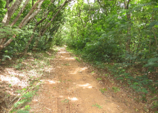
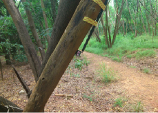
Figure 3: Left: a segment of the trail along which deployment experiments were performed. Right: the wireless nodes (TelosB motes) were latched to the trees as shown, so that all the nodes were on one side of the trail, and the line of sight between the relays passed through the foliage.

IV Radio Propagation Modeling

All our experiments were conducted on a trail in the forest-like Jubilee Gardens in the Indian Institute of Science campus (see Figure 3). Our experiments were conducted by placing the wireless devices on the edge of the trail so that the line-of-sight between the nodes passed through the foliage.

IV-A Modeling of Path-Loss and Shadowing

We kept the transmitter fixed and placed $9$ receivers along the trail at distances $50,53,56,\ldots,74$ meters respectively from the transmitter, and measured the mean received power (averaged over fading) at all receiving nodes. We repeated this with varying the transmitter location $25$ times, thereby obtaining $25$ realizations of the network with $9$ links of length $50,53,56,\cdots,74$ meters in each realization (we chose the link lengths at least $50$ meters because in reality the step size will be at least tens of meters). Under a given network realization, for the $i$-th link of length $r_{i}$ meters and shadowing realization $\nu_{i}$ dB, the mean received power in dBm (averaged over fading; see Section II-A for channel model):

$$\phi_{i}=\phi_{0}-10\eta\log\left(\frac{r_{i}}{r_{0}}\right)+\nu_{i}\>,1\leq i\leq 9$$ (4)

where $\phi_{0}$ is the mean received power (in dBm) at distance $r_{0}$.

IV-A1 Estimation of $\eta$, $\sigma$ and the shadowing decorrelation distance

According to Gudmundson’s model [10], covariance between shadowing in two different links with one end fixed and the other ends on the same line at a distance $d$ from each other can be modeled by $R_{X}(r_{i},r_{j})=\sigma^{2}\exp(-d/D)$ where $\sigma$ denotes standard deviation (in dB) of shadowing random variables, and $D$ is a constant. Let $\mathbf{\theta}:=[\phi_{0}\hskip 7.22743pt\eta\hskip 7.22743ptD\hskip 7.22743pt\sigma^{2}]$. Define $\nu_{i}^{k}$ to be the shadowing random variable for the link from the transmitter to node $i$ for the $k$-th realization of the network, where $1\leq i\leq 9$ and $1\leq k\leq 25$. Assuming that $\mathbf{\nu^{k}}:=[\nu_{1}^{k}\hskip 7.22743pt\nu_{2}^{k}\ldots\nu_{M}^{k}]^{\prime}$ is jointly Gaussian with covariance matrix denoted by $\mathbf{C(\theta)}$ (elements of this matrix are determined by Gudmundson’s model), and $\mathbf{\nu^{k}}$ is i.i.d. across $k$, we calculate the maximum likelihood estimate $\hat{\theta}_{MLE}$: $\hat{D}_{MLE}=2.6$ meters, $\hat{\sigma}_{MLE}=7.7$ dB, $\hat{\eta}_{MLE}=4.7$. The correlation coefficient of shadowing between two links is less than $0.1$ beyond $2.3D$ distance, which implies that beyond $5.98$ meters the shadowing can be safely assumed to be independent. Hence, we need $\delta\geq 6$ m.

IV-A2 Binary Hypothesis Based Approach to find the Shadowing Decorrelation Distance

The sample correlation coefficient $\hat{\rho}(r)$ between shadowing of all pairs of links whose transmitter is common and the receivers are $r$ distance apart from each other is computed as a function of $r$. We want to decide whether the shadowing losses over two links with a common receiver but whose transmitters are separated by distance $r$ are correlated. Define the null Hypotheses $H_{0}:\rho=0$ and the alternate Hypotheses $H_{1}:\rho\neq 0$. For a target false alarm probability $\alpha=0.05$ (called the significance level of the test), it turns out that we need $\hat{\rho}(r)\leq 0.34$, which requires $r\geq 3$ meters. Hence, under the jointly lognormal shadowing assumption, shadowing is independent beyond $3$ meters.

IV-A3 Testing Normality of Shadowing Random Variable via Non-Parametric Tests

We picked $25$ links from $25$ independent network realizations, and calculated their shadowing gains $\nu_{i},1\leq i\leq 25$ from (4). Then we applied Kolmogorov-Smirnov One Sample test (see [11]): define the null hypothesis $\mathcal{H}_{0}$ to be the event that the samples are coming from $\mathcal{N}(0,\hat{\sigma}_{MLE}^{2})$ distribution, and $\mathcal{H}_{1}$ to be the event that they do not. The test accepted $H_{0}$ with level of significance $0.05$. Hence, lognormal shadowing is a good model in our setting.

IV-B Number of packets to be transmitted for link evaluation

In the experiments, in order to measure the outage probability of a link, at a given transmit power a certain number of packets are sent and their RSSI values recorded. To arrive at the required number of packets we conducted the following experiment. Over several links in the field, $5000$ packets were sent at intervals of $50$ ms, and their RSSI values were recorded. We then characterise the coherence time of the fading process by modeling it as a two state process. We say that the channel is in “Bad” state when the packet RSSI falls below the mean RSSI (over packets) of the link by $20$ dB, otherwise the link is in “Good” state. From the per-packet RSSI values in the $5000$ packet experiment, we observed that the mean number of packet durations over which a channel remains in “Good” state is $56$, i.e., $2.8$ seconds, and that the mean duration of the “Bad” state is $100$ ms. Hence, we conclude that sending $2000$ packets ($100$ seconds duration, approximately $33$ Good-Bad cycles) is sufficient for the fading to be averaged out.

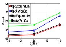
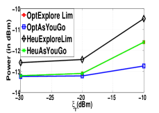
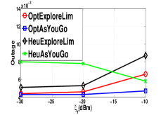
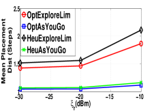
Figure 4: Model-based results for $\xi_{o}=10$: mean cost per step, mean power per link, mean outage per link and mean placement distance (steps) vs. $\xi_{r}$ for the four algorithms: OptExploreLim, OptAsYouGo, HeuExploreLim, and HeuAsYouGo. The node power in the HeuAsYouGo algorithm was taken to be the same as the mean node power with the OptExploreLim algorithm. The unit of $\xi_{r}$ is actually mW, but here it is shown in dBm.

V Numerical and Experimental Results

In this section, we use TelosB motes with $9$ dBi antenna. The set of transmit powers $\mathcal{S}=\{-25,-15,-10,-5,0\}$ dBm, and outage is the event $RSSI<-88$ dBm. We used $\eta=4.7$, $\sigma=7.7$ dB (obtained from Section IV-A), and the step size $\delta=11$ m (since the shadowing decorrelation distance is $6$ m).

Choice of $B$: Define a link to be good if its outage probability is less than $3\%$, and choose $B$ to be the largest integer such that the probability of finding a good link of length $B\delta$ is more than $20\%$, under the highest transmit power. With $\eta=4.7$ and $\sigma=7.7$ dB, $B$ turned out to be $5$.

V-A Observations from average cost per step estimates

From $\eta$ and $\sigma$, we computed $\lambda^{*}$ and $c_{th}(r)$ (see Sections III-A and III-D) for various values of $\xi_{o}$ and $\xi_{r}$, and computed for each algorithm the mean cost per step, the mean outage probability per link, the mean length of a link and the mean power per link, assuming that the channel model is specified by the values of $\eta$ and $\sigma$ computed from the experiment. We call this approach the “model-based approach” since we numerically compute the performance of the algorithms in an hypothetical homogeneous trail along which the propagation model is parameterized by the path loss exponent $\eta$ and the shadowing variance $\sigma$. We keep the HeuAsYouGo transmit power and the per-link target outage equal to the mean power per link and mean outage per link of OptExploreLim. We will only provide results for $\xi_{o}=10$; with this value the performance is satisfactory in terms of mean power per node, and the end-to-end outage for a network of length few hundreds of meters. The results are shown in Figure 4. Note that performance of OptExploreLimLearning is not shown in Figure 4, since it has the same asymptotic performance as OptExploreLim (since the policy in OptExploreLimLearning converges to the optimal policy with probability $1$).

V-A1 Mean Placement Distance

Pure as-you-go algorithms (OptAsYouGo, HeuAsYouGo of Figure 4) place relays sooner than the algorithms that explore forward before placing a relay (OptExploreLim, HeuExploreLim). This is as expected, since they do not have the advantage of exploring over several locations and then picking the best. A pure as-you-go approach tends to be cautious, and therefore tries to avoid a high outage by placing relays frequently. As $\xi_{r}$ (cost of a relay) increases, relays will be placed less frequently.

V-A2 Mean Power per Link

Increasing $\xi_{o}$ (the cost per unit outage) will lower outage and hence the transmit power increases. Increasing $\xi_{r}$ will place relays less frequently, hence the transmit power increases. OptAsYouGo has smaller placement distance compared to OptExploreLim and HeuExploreLim and hence it uses less power at each hop; we note, however, that OptAsYouGo places more relays, and, hence, could still end up using more total power.

V-A3 Mean Outage per Link

As $\xi_{o}$, the penalty for outage, increases, the mean outage per link decreases. As $\xi_{r}$ increases, the mean outage per link increases because we will place fewer relays with higher inter-relay distances. HeuAsYouGo has outage probability comparable to other algorithms, but it pays in terms of number of relays since it places relays very frequently. We observe that the per-link outage decreases with $\xi_{r}$ for HeuAsYouGo. As $\xi_{r}$ increases, the node power and the target outage (chosen from OptExploreLim) increases in such a way that the per-link outage decreases.

V-A4 Network Cost Per Step

Cost increases with $\xi_{r}$ and $\xi_{o}$. OptAsYouGo has a larger cost than OptExploreLim and HeuExploreLim, owing to shorter links. The cost of HeuAsYouGo in Figure 4 is high due to smaller placement distance. Cost of HeuExploreLim is very close to OptExploreLim.

V-B Deployment Experiments By “Virtual” Walking

Now we report our results of carrying out an experimental evaluation of all the algorithms. Based on this evaluation, we select the best algorithm and suitable parameters in order to carry out an actual impromptu deployment, which we report in Section VII. Our experimental approach is the following: (i) We deploy $11$ TelosB motes, with $9$ dBi antennas, equally spaced by $11$ meters ($\delta=11$ m), lashed to trees along one edge of a $110$ meter trail, (ii) On command, one by one, each mote broadcasts $2000$ packets at each power level from the set $\mathcal{S}=\{-25,-15,-10,-5,0\}$ dBm, while the rest remain in the receive mode. For each transmit power level of a node, the outage probability at each other receiving node is recorded.

Next, we applied the policies to the data. Since we have gathered the outage probabilities of every possible link for all power levels, we have all possible measurements that can be possibly made during an actual deployment. Thus, we can use the measurements to determine the actual network that will be deployed if an agent was to walk along the trail starting from sink at location 1, with the source being at location 11 (the distance between the sensor and the base station is $110$ meters). We choose $\xi_{o}=10$ and $\xi_{r}=0.01$ for the virtual deployment. For the HeuAsYouGo algorithm, we randomized between two power levels from $\mathcal{S}$ so that the mean transmit power per node in the data-based HeuAsYouGo remains equal to that of model-based OptExploreLim. We have also calculated the optimal end-to-end cost of the network graph; we calculated the shortest path from node $11$ to node $1$ over the weighted network graph where the weight of any potential link consists of the transmit power, outage cost and relay cost, and the weights are available from the field measurements. The cost of the sensor node is not taken into account. Obviously, this approach (OptExploreAll) gives the smallest end-to-end cost (see Table I and the abbreviations in its caption). If we place a relay at location $i$, ($i\geq 7$), the remaining number of steps from there to the sensor location is less than $B=5$. In that case, we place one more relay between locations $i$ and $11$ such that the cost between $11$ and $i$ is minimized. For OptExploreLimLearning, we chose $\lambda_{0}=0.0321$ (optimal cost per step when $\eta=4$, $\sigma=7$ dB).

Algo-	Relay	No. of mea-	Total Po-	Sum	Total
rithm	location	surements	wer (mW)	Outage	Cost
OEL	5,7,9	17	0.3542	0.004	0.424
HEL	5,7,9	17	0.3542	0.004	0.424
OELL	4,8,10	15	0.3826	0.006	0.472
OAYG	2,3,4,5,6,8,9	10	0.747	0.018	0.997
HAYG	2,3,5,6,7,	10	0.451	0.586	6.391
	8,9,10
OEA	2,6,9	40	0.0704	0.002	0.1204

TABLE I: Results of virtual walking deployment for one side of a trail, for $\xi_{r}=0.01$ and $\xi_{o}=10$. Abbreviations: OEL-OptExploreLim, HEL-HeuExploreLim, OELL-OptExploreLimLearning, OAYG-OptAsYouGo, HAYG-HeuAsYouGo, OEA-OptExploreAll.

The OptExploreLim algorithm places relays at locations 5,7,9. It requires $B=5$ measurements for placing at each of $5$ and $7$, see Table I. Then it has to place one more relay, for that it has to measure the cost of the following paths: $\{(11,10),(10,7)\}$, $\{(11,9),(9,7)\}$, $\{(11,8),(8,7)\}$ and $(7,7)$. Hence, OptExploreLim requires $17$ measurements to place 3 relays. Similar logic follows for HeuExploreLim and OptExploreLimLearning. The as-you-go algorithms require $10$ measurements for $10$ steps, and place 7-8 relays. Exploration algorithms place a smaller number of relays and yet produce much better performance compared to pure as-you-go. OptExploreAll (the best algorithm) significantly improves the performance compared to exploration algorithms, but makes $40$ measurements (between all potential location pairs whose distance is less than or equal to $5$ steps). As-you-go algorithms work with measurements acquired as the agent walks and, hence, are suboptimal. Hence, the algorithms that employ partial exploration are the ones that require reasonable number of measurements while giving satisfactory performance.

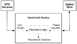
Figure 5: Architecture of the deployment tool (basically a notebook computer with a GPS dongle and a Zigbee mote (the commanding node (CN); see text) attached via a USB port).

VI Implementation for Actual Deployment

In Section V-B we provided results from "virtual walking" deployments which are basically off-line computations that utilised detailed field measurements of all possible potential links in the field. We next turn to our experiments with "actual walking" deployments. The deployment agent carrying a deployment tool (see Figure 5) goes about executing the process described here starting from the base station and proceeds all the way to the location where the sensor has to be placed. On the way, the relay nodes are placed as guided by the placement algoithm running on the deployment tool. The previously Placed Node (PPN) is the most recently placed node in the deployment. The evaluation node (EN) is the node that is evaluated by the placement algorithm; it is lashed to a tree at (or just near) a potential placement point (i.e., a multiple of $\delta$ steps from the PPN). The commanding node (CN) is the command relay node which is attached to the deployment tool from which the deployment agent will issue commands for evaluation. At a potential location, the agent issues a command to the EN via CN to evaluate the link between EN and PPN. After performing link quality measurements such as link outage, at different transmit power levels, the EN reports the results to the CN. After evaluating the requisite number of EN locations (one for pure as-you-go deployment, and $B$ for exploration based algorithms), the placement algorithm decides where the EN should be placed. The procedure is repeated until the source location is reached.

The mote side of the deployment code is written in TinyOS and the node placement code uses C and Matlab. In hardware, the deployment tool consists of a USB GPS receiver, a mote, and a handheld device (netbook running Fedora 12 distribution) that can interface with the GPS and the mote (Figure 5). We have used a low cost off-the-shelf GPS USB receiver dongle for getting the location information. This receiver is based on the SiRF STAR III chipset. In our GPS experiments, we got an error of roughly 5 meters for less than 50 meters distance in the best case where there is a clear sky and good satellite visibility. Considering that practical deployment distances would be much higher than 50 meters (particularly with high power motes), we found that the GPS error is within the acceptable limits.

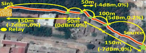
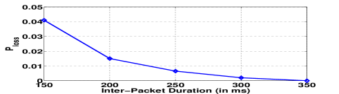
Figure 6: Real deployment along a long trail using OptExploreLimLearning with iWiSe motes, $\xi_{o}=100$, $\xi_{r}=1$: five nodes (including the source) are placed; link lengths, transmit powers, and $\%$ outage probabilities are shown; the plot shows variation of end-to-end loss probability with inter-packet duration for periodically generated packets from the source

VII Physical Deployment Experiments

With the experience (on the choice of deployment algorithm) obtained from the virtual deployment experiment discussed in Section V, we performed some real deployment experiments along a long trail in our campus (not exactly linear in shape, which is the reality in a practical forest environment) with the powerful iWiSe motes (see [12]) equipped with $9$ dBi antennas. We chose $\xi_{o}=100$, $\xi_{r}=1$, $B=5$ steps, $\delta=50$ meters, and $\mathcal{S}=\{-7,-4,0,5\}$ dBm. $P_{rcv-min}=-97$ dBm; the PER at this RSSI becomes $2\%$ for iWiSe motes (obtained experimentally). In this deployment experiment we used the PER of a link as a substitute for outage probability; this does not violate the basic assumptions of our formulation, and the algorithms remain the same. For $\eta=4$, $\sigma=7$ dB, the optimal average cost per step is $1.0924$ (computed numerically using policy iteration). Taking $\lambda_{0}=1.0924$ (the initial guess), we performed real deployment experiments with OptExploreLimLearning. The deployed network is shown in Figure 6. The sink is denoted by the “house” symbol. The two short ($50$ m long) links account for significant path-loss due to the turn in the trail. After completion of the deployment, we used the last placed node as the source and sent periodic traffic from the source to the sink node at various rates. As the arrival rate increases, the loss probability increases (see Figure 6) due to carrier sense failures and collisions because of simultaneous transmissions from different nodes. For very low arrival rate, the loss probability becomes $0$ even though the sum PER under the lone packet model is not $0$. This happens because of link level retransmissions and the relatively short outage durations; even if a packet encounters an outage on a link along the path, retransmission attempts succeed with high probability. We see that, even though the design was for the lone packet model, the network can carry $4$ packets/second with $P_{loss}\leq 1\%$.

VIII Conclusion and Ongoing Work

In this paper, we have compared the on-field performance of several as-you-go deployment algorithms. Pure as-you-go networks need to be overly cautious, and, hence, deploy far too many relays. Our results suggest that limited exploration based on-line algorithms (such as HeuExploreLim, and OptExploreLimLearning) provide satisfactory performance, at the cost of some additional measurements. In a large forest, we can deploy using OptExploreLimLearning in one trail and use the updated policy in another trail so that the per-step cost of the entire network is optimal. There are several issues left for future study: (i) robust deployment against seasonal variation of propagation, and (ii) deployment in 2D and 3D regions.

References

- [1] A. Chattopadhyay, M. Coupechoux, and A. Kumar. As-you-go deployment of a wireless network with on-line measurements and backtracking. http://arxiv.org/abs/1308.0686.
- [2] A. Chattopadhyay, M. Coupechoux, and A. Kumar. Measurement based impromptu deployment of a multi-hop wireless relay network. In Proc. of the 11th Intl. Symposium on Modeling and Optimization in Mobile, Ad Hoc, and Wireless Networks (WiOpt). IEEE, 2013.
- [3] M.R. Souryal, J. Geissbuehler, L.E. Miller, and N. Moayeri. Real-time deployment of multihop relays for range extension. In Proc. of the ACM International Conference on Mobile Systems, Applications and Services (MobiSys), San Juan, Puerto Rico, June 2007, pages 85–98. ACM, 2007.
- [4] H. Liu, J. Li, Z. Xie, S. Lin, K. Whitehouse, J.A. Stankovic, and D. Siu. Automatic and robust breadcrumb system deployment for indoor firefighter applications. In Proc. of the ACM International Conference on Mobile Systems, Applications and Services (MobiSys), 2010.
- [5] T. Aurisch and J. Tölle. Relay Placement for Ad-hoc Networks in Crisis and Emergency Scenarios. In Proc. of the Information Systems and Technology Panel (IST) Symposium. NATO Science and Technology Organization, 2009.
- [6] M. Howard, M.J. Matarić, and S. Sukhat Gaurav. An incremental self-deployment algorithm for mobile sensor networks. Kluwer Autonomous Robots, 13(2):113–126, 2002.
- [7] A. Sinha, A. Chattopadhyay, K.P. Naveen, M. Coupechoux, and A. Kumar. Optimal sequential wireless relay placement on a random lattice path. Ad Hoc Networks Journal (Elsevier)., 21:1–17, 2014.
- [8] A. Bhattacharya, A. Rao, D. G. Rao Sahib, A. Mallya, S.M. Ladwa, R. Srivastava, S.V.R. Anand, and A. Kumar. Smartconnect: A system for the design and deployment of wireless sensor networks. In Proc. of the 5th International Conference on Communication Systems and Networks (COMSNETS). IEEE, 2013.
- [9] A. Bhattacharya and A. Kumar. QoS aware and survivable network design for planned wireless sensor networks. http://arxiv.org/abs/1110.4746.
- [10] M. Gudmundson. Correlation model for shadow fading in mobile radio systems. In Electronics letters, volume 27, pages 2145–2146. IET, 1991.
- [11] P.J. Bickel and K.A. Doksum. Mathematical Statistics, volume I. Prentice Hall Englewood Cliffs, NJ, 2001.
- [12] http://www.astec.org.in/astec/content/wireless-sensor-network,.