Shell model and deformed shell model spectroscopy of ⁶²Ga

Abstract

In the present work we have reported comprehensive analysis of recently available experimental data [H.M. David et al., Phys. Lett. B 726, 665 (2013)] for high-spin states up to $17^{+}$ with $T=0$ in the odd-odd $N=Z$ nucleus ⁶²Ga using shell model calculations within the full $f_{5/2}pg_{9/2}$ model space and deformed shell model based on Hartee-Fock intrinsic states in the same space. The calculations have been performed using jj44b effective interaction developed recently by B.A. Brown and A.F. Lisetskiy for this model space. The results obtained with the two models are similar and they are in reasonable agreement with experimental data. In addition to the $T=0$ and $T=1$ energy bands, band crossings and electromagnetic transition probabilities, we have also calculated the pairing energy in shell model and all these compare well with the available theoretical results.

1 Introduction

In the recent past there are many experimental and theoretical investigations for heavy $N=Z$ nuclei. In the case of even-even $N=Z$ nuclei from ⁶⁸Se ($Z=34$) to ⁸⁸Ru ($Z=44$) many interesting phenomena have been observed. For example, ⁶⁸Se exhibits oblate shape in the ground state se68 and in the case of ⁷²Kr 72kr shape-coexistence has been observed. On the other hand, the nuclei ⁷⁶Sr76sr and ⁸⁰Zr80zr have large ground-state deformation. Also, the even-even N=Z nuclei are waiting point nuclei for $rp$-process nucleosynthesis. As we move further, there is a decrease in deformation as seen for example in ⁸⁴Mo84mo and ⁸⁸Ru88ru . However, more interesting are the N=Z odd-odd nuclei as they will allow us to investigate isospin effects and in particular about $T=0$ vs $T=1$ pairing. As a consequence there are continuous experimental efforts to study in detail odd-odd N=Z nuclei in the A $\sim$ 60-80 region Vin ; rudolph ; david ; as66 ; br70 ; rb74a ; rb74b ; rb74c ; y78 ; 62gaprl . In this paper we will consider ⁶²Ga where there are new and more complete data david obtained recently by using heavy-ion fusion-evaporation reaction ⁴⁰Ca(²⁴Mg,$pn$)⁶²Ga near the Coulomb barrier with ATLAS accelerator and Gammasphere array. These data go much beyond the data reported previously in 1998 Vin and 2004 rudolph on $T=0$ and $T=1$ levels in this nucleus. Theoretical results for low-lying T=0 and T=1 states, with low spins, of ⁶²Ga obtained using SM sm2 , DSM dsm and IBM-4 sm2 are available in the literature. In the previous SM and DSM calculations realistic G-matrix interaction with a phenomenologically adjusted monopole part as given by the Madrid-Strasbourg group No-01 has been used. More recently, Shell Model using Madrid-Strasbourg effective interaction and Cranked Nilsson-Strutinsky model calculations for yrast states of ⁶²Ga have been performed npa . The aim of the present study is to explain, more comprehensively, the recent experimental data for ⁶²Ga using shell model (SM) calculations and also extend the deformed shell model (DSM) (based on Hartree-Fock states) calculations reported in the past for this nucleus dsm both with a more recently introduced effective interaction jj44b jj44b . In the present work we have not only focused on low-lying levels but also on high-spin states up to $17^{+}$ with $T=0$.

The paper is organized as follows. Section 2 gives some details regarding the effective interaction used and about DSM. Section 3 gives results from SM and DSM and their comparison with experimental data. Comparison with previous theoretical studies is given in section 4. Finally, concluding remarks are drawn in section 5.

2 Method of Calculations

In the present work for both SM and DSM, ⁵⁶Ni is taken as the inert core with the spherical orbits $2p_{3/2}$, $1f_{5/2}$, $2p_{1/2}$ and $1g_{9/2}$ as active orbits. The jj44b interaction due to Brown and Lisetskiy jj44b was employed in the calculations. This interaction was developed by fitting 600 binding energies and excitation energies from nuclei with $Z=28-30$ and $N=48-50$. Here, 30 linear combinations of $JT$ coupled two-body matrix elements (TBME) are varied giving the rms deviation of about 250 keV from experiment. The single particle energies (spe) are taken to be jj44b -9.6566, -9.2859, -8.2695 and -5.8944 MeV for the $p_{3/2}$, $f_{5/2}$, $p_{1/2}$ and $g_{9/2}$ orbits respectively. The shell model calculations are carried out using the shell model code NuShell nushell . The maximum matrix dimension in $M$-scheme is for $0^{+}$ states and it is $91564$.

Turning to DSM, for a given nucleus, starting with a model space consisting of the given set of single particle (sp) orbitals and effective two-body Hamiltonian (TBME + spe), the lowest energy intrinsic states are obtained by solving the Hartree-Fock (HF) single particle equation self-consistently. Excited intrinsic configurations are obtained by making particle-hole excitations over the lowest intrinsic state. These intrinsic states $\chi_{K}(\eta)$ do not have definite angular momenta. and states of good angular momentum projected from an intrinsic state $\chi_{K}(\eta)$ can be written in the form

$$\psi^{J}_{MK}(\eta)=\frac{2J+1}{8\pi^{2}\sqrt{N_{JK}}}\int d\Omega D^{J^{*}}_{MK}(\Omega)R(\Omega)|\chi_{K}(\eta)\rangle$$ (1)

where $N_{JK}$ is the normalization constant given by

$$N_{JK}=\frac{2J+1}{2}\int^{\pi}_{0}d\beta\sin\beta d^{J}_{KK}(\beta)\langle\chi_{K}(\eta)|e^{-i\beta J_{y}}|\chi_{K}(\eta)\rangle$$ (2)

In Eq. (1) $\Omega$ represents the Euler angles ($\alpha$, $\beta$, $\gamma$), $R(\Omega)$ which is equal to exp($-i\alpha J_{z}$)exp($-i\beta J_{y}$)exp( $-i\gamma J_{z}$) represents the general rotation operator. The good angular momentum states projected from different intrinsic states are not in general orthogonal to each other. Hence they are orthonormalized and then band mixing calculations are performed. In addition, as required for N=Z nuclei, isospin projection is also included in DSM. For details see for example SSK ; KS1 ; KS2 ; KS3 . DSM is well established to be a successful model for transitional nuclei (with A=60-90) when sufficiently large number of intrinsic states are included in the band mixing calculations.

For ⁶²Ga nucleus, fig. 1 gives the HF single particle (sp) spectrum (the states are labeled by $|k_{\alpha}\rangle$ where the $\alpha$ label distinguishes different states with the same $k$ value) for both prolate and oblate solution. As seen from the figure, the prolate solution is lowest. The lowest HF intrinsic state from the prolate solution consists of two protons and two neutrons occupying the lowest $k=1/2^{-}$ state and the last unpaired odd proton and neutron occupying the next $k=1/2^{-}$ state. The HF energy ($E$), the mass quadrupole moment ($Q$) and band $K$-value are also shown in the figure. For the four nucleons (two protons and two neutrons) occupying the lowest $k=1/2^{-}$ sp state we have $T=0$. Hence the isospin for ⁶²Ga is determined by the last proton and neutron. Thus the total isospin for the configuration shown in fig. 1 is $T=0$ as the odd proton and odd neutron, for $K=1^{+}$, form a symmetric pair in the $k$-space (here and elsewhere in this paper symmetry in $k$-space means symmetry in space-spin co-ordinates as $k$ contains both space (orbital) and spin co-ordinates). Particle-hole excitations over the lowest HF intrinsic state (from both prolate and oblate solutions) generate excited HF intrinsic states. There are 44 low-lying excited intrinsic states obtained by particle-hole excitation up to 3 MeV excitation. The HF intrinsic states are in general admixtures of various isospin components. As mentioned above, the lowest prolate and oblate HF intrinsic states will have $T=0$. If in an excited intrinsic state, the unpaired proton occupies the single particle orbit specified by the azimuthal quantum number $k_{1}$ and the unpaired neutron occupies the state $k_{2}$, then one can also consider an intrinsic state where the occupancies of the unpaired nucleons are reversed. By taking a linear combination of these intrinsic states, one can construct intrinsic states which are symmetric (or antisymmetric) in $k$-space co-ordinates and they correspond to $T=0$ and $T=1$ states respectively. With this isospin projection, in the present calculation, there are 26 intrinsic states for $T=0$ and 18 for $T=1$ (total 44). All the configurations are listed in table 1. Then good angular momentum states are projected from all the $T=0$ intrinsic states and a band mixing calculation is performed. Similar procedure is also applied for the $T=1$ intrinsic states.

3 Results and discussions

3.1 Shell model results

Fig. 2 shows comparison of recently available experimental data david with SM for the spectra with the lowest $T=1$ band and three higher $T=0$ bands with maximum spin $17^{+}$. The agreements are reasonable. However, the SM gives the excitation energy of the lowest $T=0$ level (with $1^{+}$) to be 148 keV against the experimental value 571 keV. In order to bring out the structure of these levels, in table 2 given are the dominant shell model configuration (and its probability) in a given level and also the occupancies of the four single particle orbits. In the lowest $T=0$ band, the high-spin levels starting from $J^{\pi}=13^{+}$ have $g_{9/2}$ occupancy close to $2$ while the lower levels are essentially from the $f_{5/2}p$ orbits. For example, the structure changes from $1^{+}$ with dominant configuration $f_{5/2}^{3}p_{3/2}^{3}$ ($\sim$ 14.66%) to $17^{+}$ with dominant configuration $f_{5/2}^{2}p_{3/2}^{2}g_{9/2}^{2}$ ($\sim$ 68.87%). This shows that as we move to higher $J$ values, the $g_{9/2}^{2}$ orbital start playing an important role in the structure. It is also seen from table 2 that the second $T=0$ band is essentially from $f_{5/2}p$ orbits for spins up to $10^{+}$ while for the third band $g_{9/2}$ is important for the $10^{+}$ level. Turning to yrast T=1 states, it is seen that shell model gives very good agreement with available experimental data. The structure of $0^{+}$ to $10^{+}$ levels is mainly due to $(f_{5/2}p_{3/2}p_{1/2})^{6}$ configuration and the structure of low $J$ values is more fragmented in comparison to high $J$ values. This is reflected from the change in the probability $\sim$ 17.93% ($0^{+}$) to $\sim$ 65.15% ($10^{+}$ ).

There is interest in the number of low-lying (say up to 2 or 3 MeV) states in odd-odd N=Z nuclei compared to the neighboring neutron-rich odd-odd nuclei. For example, the ⁶²Ga with N=Z has much lower number of levels up to 1.7 MeV excitation compared to those in ⁶⁴Ga ($\sim 30$ levels) and ⁶⁸Ga ($\sim 60$ levels); see the discussion in david . Because of this important issue, we show in fig. 3 all the low-lying levels up to 3 MeV excitation. It is seen that the sequence of lowest-lying states is well reproduced by shell model although the calculated level energies are compressed.

Finally, some results for $B(E2)$’s are shown in table 3 and for $B(M1)$’s in table 4. For $T=0$ state the B(E2,$3_{1}^{+}\rightarrow 1_{1}^{+}$) from shell model is 6.43 W.u. while the corresponding experimental value is 12 W.u. The result may improve if we slightly increase the effective charges. Similarly, the $B(M1)$ is largest for the $0^{+}_{1}$ of $T=1$ to $1^{+}_{1}$ of $T=0$. Further discussion is given below.

Figure 1: HF single particle spectra for ⁶²Ga corresponding to lowest prolate and oblate configurations. In the figures circles represent protons and crosses represent neutrons. The Hartree-Fock energy ($E$) in MeV, mass quadrupole moment ($Q$) in units of the square of the oscillator length parameter and the total $K$ quantum number of the lowest intrinsic states are given in the figure.

Table 1: Intrinsic states used for ⁶²Ga in DSM calculation. For each intrinsic state, given are the corresponding configurations, the total $K$-quantum number and isospin ($T$). The states 1 to 20 are prolate configurations and 21 to 26 oblate. Superscript $(2p,2n)$ implies that the orbit is occupied by two protons and two neutrons and similarly the superscript $(p,n)$. In addition, the superscripts $p(n)$ and $n(p)$ imply that the orbit(s) is(are) alternatively occupied by a proton and a neutron or a neutron and a proton.

No.	$\;\;K\;\;$	$\;\;T$	Configuration
1.	$1^{+}$	0	$(1/2^{-})_{1}^{2p,2n}(1/2^{-}\uparrow)_{2}^{p,n}$
2.	$0^{+}$	0,1	$(1/2^{-})_{1}^{2p,2n}(1/2^{-}\uparrow)_{2}^{p(n)}(1/2^{-}\downarrow)_{2}^{n(p)}$
3.	$3^{+}$	0	$(1/2^{-})_{1}^{2p,2n}(3/2^{-}\uparrow)_{1}^{p,n}$
4.	$0^{+}$	0,1	$(1/2^{-})_{1}^{2p,2n}(3/2^{-}\uparrow)_{1}^{p(n)}(3/2^{-}\downarrow)_{1}^{n(p)}$
5.	$1^{+}$	0,1	$(1/2^{-})_{1}^{2p,2n}(3/2^{-}\uparrow)_{1}^{p(n)}(1/2^{-}\downarrow)_{2}^{n(p)}$
6.	$2^{+}$	0,1	$(1/2^{-})_{1}^{2p,2n}(3/2^{-}\uparrow)_{1}^{p(n)}(1/2^{-}\uparrow)_{2}^{n(p)}$
7.	$3^{+}$	0	$(1/2^{-})_{1}^{2p,2n}(3/2^{-}\uparrow)_{2}^{p,n}$
8.	$0^{+}$	0,1	$(1/2^{-})_{1}^{2p,2n}(3/2^{-}\uparrow)_{2}^{p(n)}(3/2^{-}\downarrow)_{2}^{n(p)}$
9.	$1^{+}$	0,1	$(1/2^{-})_{1}^{2p,2n}(3/2^{-}\uparrow)_{2}^{p(n)}(1/2^{-}\downarrow)_{2}^{n(p)}$
10.	$2^{+}$	0,1	$(1/2^{-})_{1}^{2p,2n}(3/2^{-}\uparrow)_{2}^{p(n)}(1/2^{-}\uparrow)_{2}^{n(p)}$
11.	$0^{+}$	0,1	$(1/2^{-})_{1}^{2p,2n}(3/2^{-}\uparrow)_{2}^{p(n)}(3/2^{-}\downarrow)_{1}^{n(p)}$
12.	$3^{+}$	0,1	$(1/2^{-})_{1}^{2p,2n}(3/2^{-}\uparrow)_{2}^{p(n)}(3/2^{-}\uparrow)_{1}^{n(p)}$
13.	$1^{+}$	0	$(1/2^{-})_{1}^{2p,2n}(1/2^{+}\uparrow)_{1}^{p,n}$
14.	$0^{+}$	0,1	$(1/2^{-})_{1}^{2p,2n}(1/2^{+}\uparrow)_{1}^{p(n)}(1/2^{+}\downarrow)_{1}^{n(p)}$
15.	$3^{+}$	0	$(1/2^{-})_{1}^{2p,2n}(3/2^{+}\uparrow)_{1}^{p,n}$
16.	$0^{+}$	0,1	$(1/2^{-})_{1}^{2p,2n}(3/2^{+}\uparrow)_{1}^{p(n)}(3/2^{+}\downarrow)_{1}^{n(p)}$
17.	$1^{+}$	0,1	$(1/2^{-})_{1}^{2p,2n}(3/2^{+}\uparrow)_{1}^{p(n)}(1/2^{+}\downarrow)_{1}^{n(p)}$
18.	$2^{+}$	0,1	$(1/2^{-})_{1}^{2p,2n}(3/2^{+}\uparrow)_{1}^{p(n)}(1/2^{+}\uparrow)_{1}^{n(p)}$
19.	$1^{+}$	0	$(1/2^{-})_{2}^{2p,2n}(1/2^{-}\uparrow)_{1}^{p,n}$
20.	$0^{+}$	0,1	$(1/2^{-})_{2}^{2p,2n}(1/2^{-}\uparrow)_{1}^{p(n)}(1/2^{-}\downarrow)_{1}^{n(p)}$
21.	$5^{+}$	0	$(3/2^{-})_{1}^{2p,2n}(5/2^{-}\uparrow)_{1}^{p,n}$
22.	$0^{+}$	0,1	$(3/2^{-})_{2}^{2p,2n}(5/2^{-}\uparrow)_{1}^{p(n)}(5/2^{-}\downarrow)_{1}^{n(p)}$
23.	$1^{+}$	0	$(3/2^{-})_{1}^{2p,2n}(1/2^{-}\uparrow)_{1}^{p,n}$
24.	$0^{+}$	0,1	$(3/2^{-})_{1}^{2p,2n}(1/2^{-}\uparrow)_{1}^{p(n)}(1/2^{-}\downarrow)_{1}^{n(p)}$
25.	$3^{+}$	0,1	$(3/2^{-})_{1}^{2p,2n}(5/2^{-}\uparrow)_{1}^{p(n)}(1/2^{-}\uparrow)_{1}^{n(p)}$
26.	$2^{+}$	0,1	$(3/2^{-})_{1}^{2p,2n}(5/2^{-}\uparrow)_{1}^{p(n)}(1/2^{-}\downarrow)_{1}^{n(p)}$

3.2 Deformed shell model results

Figs. 2 and 3 shows comparison of DSM results with experimental data david and SM for high spin states and all low-lying levels respectively. The agreements between experiment and DSM and also between DSM and SM are reasonable. As discussed in KS1 , DSM can produce only the relative energies in the $T=0$ levels and similarly for the $T=1$ levels. Following this, all the $T=0$ levels are pushed up by 600 keV (experimental value is 571 keV with respect to the lowest $T=1$ level just as in KS1 ; KS2 ). For the lowest $T=0$ band (see fig. 1) it is seen that there is a band crossing at $11^{+}$ with clear structural change from $13^{+}$. The $13^{+}$, $15^{+}$ and $17^{+}$ mainly originate from the rotational aligned $K=1^{+}$ band obtained by placing a proton (neutron) in a $k=3/2^{+}$ and neutron (proton) in a $k=1/2^{+}$ orbit. This corresponds to the configuration number 17 in table 1. This configuration given by DSM is consistent with SM result as given table 2, i.e. the high-spin levels from $13^{+}$ have $g_{9/2}$ occupancy $\sim 2$. The levels below $11^{+}$ are essentially from $f_{5/2}p$ orbits (as in SM, see table 2) dominated by the deformed configurations #1, #2 and #4 in table 1. As seen from the fig. 2, there are two close-lying $9^{+}$ levels with $T=0$ (this is seen for $9^{+}$ in experimental data) and the $9^{+}_{1}$ arise from the mixing of the configurations #1 and #10 (close in structure to $7^{+}_{1}$) while $9^{+}_{2}$ arise from mixing of configurations #1 and #6. The SM has also two $9^{+}$ levels as shown in fig. 2. From the $B(E2)$ values shown in table 3 for $9^{+}_{i}\rightarrow 7^{+}_{1}$ it is clear, as we expect large $B(E2)$ value with the levels belonging to the same band, that the $9^{+}_{1}$ (5075 keV) of DSM should correspond to $9^{+}_{2}$ (5405 keV) of SM. For the two $11^{+}$ levels in DSM, there is considerable mixing of various configurations. From the $13^{+}_{1}\rightarrow 11^{+}_{i}$ $B(E2)$ values shown in table 3 and that there is clear structural change after $11^{+}$ allow as to conclude that the $11^{+}_{2}$ (6311 keV) of DSM corresponds to $11^{+}_{2}$ (7421 keV) of SM (see fig. 2). With these correspondence between DSM and SM we expect the $B(E2)$ for $11^{+}_{2}\rightarrow 9^{+}_{1}$ of DSM should be close to that of $11^{+}_{2}\rightarrow 9^{+}_{2}$ of SM. This is indeed seen in table 3 (DSM gives 0.4 W.u. and SM gives 1.05 W.u.). Thus we have a good correspondence between the yrast $T=0$ levels in DSM and SM.

Going to the non-yrast $T=0$ bands shown in fig. 2, the first excited $2^{+}$ band like structure is mainly from configurations #5 and #6 and the second $2^{+}$ band arises mainly from configuration #1 shown in table 1. Going to the $T=1$ band, this arises mainly from configurations #2 and #4. It is also seen that with increase in spin in the band, there more mixing of other deformed configurations (therefore SM configurations at higher spins are more pure as stated in Section 3.1). The $B(E2)^{\prime}s$ values from DSM and SM are similar for the $T=1$ band and the collectivity starts decreasing from $6^{+}$. For the $10^{+}\rightarrow 8^{+}$, the DSM value is much smaller than SM value. In addition, table 4 gives $B(M1)$ values for some of yrast $T=1$ to yrast $T=0$ transitions. It is seen that the $0^{+}_{1}\rightarrow 1^{+}_{1}$ transition is strong and the DSM value is close to SM value. Other transition strengths are much smaller in both models.

Turning to the low-lying levels, all levels (with $T=0$ and $T=1$) predicted by DSM below 3 MeV excitation are compared with SM and experimental data in fig. 3. The number of levels in the experiment, SM and DSM with $T=0$ up to $1.7$ MeV are 7, 17 and 10. As mentioned before, the experimentally observed level density up to $1.7$ MeV excitation in the neighboring odd-odd Ga isotopes is much larger. Another important feature is that in the $T=0$ levels, the experimental data show a well defined gap of $\sim 600$ keV above 1.575 MeV level. A similar gap is seen in both DSM and SM. Also, the $2_{2}^{+}$, $0^{+}_{2}$ and $3^{+}_{1}$ of $T=1$ shown in fig. 3 for DSM (also SM) are indeed seen in the isobaric analogue nucleus ⁶²Zn.

Table 2: Shell model configurations and occupancies for $T=0$ and $T=1$ levels.

T=0	% probability	configurations	nucleon occupation numbers
			$n_{lj}^{\pi}$ = $n_{lj}^{\nu}$ ($f_{5/2}$,$p_{3/2}$, $p_{1/2}$,$g_{9/2}$)
$1^{+}$	14.66	$f_{5/2}^{3}$ $p_{3/2}^{3}$ $p_{1/2}^{0}$ $g_{9/2}^{0}$	1.71  3.08  1.00  0.21
$3^{+}$	24.18	$f_{5/2}^{2}$ $p_{3/2}^{3}$ $p_{1/2}^{1}$ $g_{9/2}^{0}$	2.12  2.76  0.92  0.21
$5^{+}$	30.30	$f_{5/2}^{2}$ $p_{3/2}^{4}$ $p_{1/2}^{0}$ $g_{9/2}^{0}$	2.22  2.74  0.79  0.24
$7^{+}$	32.38	$f_{5/2}^{2}$ $p_{3/2}^{3}$ $p_{1/2}^{1}$ $g_{9/2}^{0}$	2.21  2.82  0.78  0.19
$9^{+}$	32.94	$f_{5/2}^{2}$ $p_{3/2}^{4}$ $p_{1/2}^{0}$ $g_{9/2}^{0}$	2.32  2.97  0.59  0.11
$13^{+}$	34.78	$f_{5/2}^{3}$ $p_{3/2}^{1}$ $p_{1/2}^{0}$ $g_{9/2}^{2}$	2.29  1.16  0.49  2.05
$11^{+}$	94.59	$f_{5/2}^{4}$ $p_{3/2}^{2}$ $p_{1/2}^{0}$ $g_{9/2}^{0}$	3.94  1.94  0.01  0.11
$15^{+}$	36.50	$f_{5/2}^{2}$ $p_{3/2}^{1}$ $p_{1/2}^{1}$ $g_{9/2}^{2}$	2.22  1.25  0.50  2.03
$17^{+}$	68.87	$f_{5/2}^{2}$ $p_{3/2}^{2}$ $p_{1/2}^{0}$ $g_{9/2}^{2}$	2.33  1.65  0.00  2.02
$2^{+}$	14.57	$f_{5/2}^{1}$ $p_{3/2}^{4}$ $p_{1/2}^{1}$ $g_{9/2}^{0}$	1.87  2.97  0.94  0.21
$4^{+}$	15.27	$f_{5/2}^{2}$ $p_{3/2}^{3}$ $p_{1/2}^{1}$ $g_{9/2}^{0}$	2.02  2.91  0.84  0.23
$6^{+}$	17.89	$f_{5/2}^{3}$ $p_{3/2}^{3}$ $p_{1/2}^{0}$ $g_{9/2}^{0}$	2.62  2.43  0.70  0.25
$8^{+}$	45.66	$f_{5/2}^{3}$ $p_{3/2}^{3}$ $p_{1/2}^{0}$ $g_{9/2}^{0}$	3.04  2.27  0.45  0.23
$10^{+}$	69.08	$f_{5/2}^{3}$ $p_{3/2}^{3}$ $p_{1/2}^{0}$ $g_{9/2}^{0}$	3.09  2.64  0.16  0.10
$2^{+}$	16.24	$f_{5/2}^{3}$ $p_{3/2}^{2}$ $p_{1/2}^{1}$ $g_{9/2}^{0}$	2.44  2.45  0.89  0.22
$4^{+}$	18.51	$f_{5/2}^{0}$ $p_{3/2}^{5}$ $p_{1/2}^{1}$ $g_{9/2}^{0}$	1.66  3.19  0.92  0.22
$6^{+}$	30.12	$f_{5/2}^{3}$ $p_{3/2}^{3}$ $p_{1/2}^{0}$ $g_{9/2}^{0}$	2.29  2.93  0.58  0.20
$8^{+}$	26.35	$f_{5/2}^{2}$ $p_{3/2}^{3}$ $p_{1/2}^{1}$ $g_{9/2}^{0}$	3.03  2.42  0.44  0.11
$10^{+}$	31.27	$f_{5/2}^{4}$ $p_{3/2}^{0}$ $p_{1/2}^{0}$ $g_{9/2}^{2}$	2.90  0.91  0.28  1.90
T=1
$0^{+}$	17.93	$f_{5/2}^{2}$ $p_{3/2}^{4}$ $p_{1/2}^{0}$ $g_{9/2}^{0}$	1.89  2.85  0.81  0.43
$2^{+}$	14.07	$f_{5/2}^{2}$ $p_{3/2}^{3}$ $p_{1/2}^{1}$ $g_{9/2}^{0}$	2.09  2.65  0.90  0.35
$4^{+}$	17.23	$f_{5/2}^{3}$ $p_{3/2}^{3}$ $p_{1/2}^{0}$ $g_{9/2}^{0}$	2.53  2.41  0.74  0.33
$6^{+}$	17.58	$f_{5/2}^{3}$ $p_{3/2}^{3}$ $p_{1/2}^{0}$ $g_{9/2}^{0}$	2.78  2.35  0.64  0.24
$8^{+}$	24.55	$f_{5/2}^{3}$ $p_{3/2}^{3}$ $p_{1/2}^{0}$ $g_{9/2}^{0}$	2.86  2.50  0.44  0.19
$10^{+}$	65.15	$f_{5/2}^{3}$ $p_{3/2}^{3}$ $p_{1/2}^{0}$ $g_{9/2}^{0}$	3.28  2.59  0.14  0.11

Table 3: $B(E2)$ values (in W.u.) in SM and DSM obtained using effective charges $e_{p}=1.5e$ and $e_{n}=0.5e$. Experimental value (shown in the last column) is taken from the NNDC database.

$I_{f}^{+}\rightarrow I_{i}^{+}$	DSM	SM	EXPT.
T=0 (Isoscalar)
$3_{1}^{+}\rightarrow 1_{1}^{+}$	24.7	6.46	12${}^{+6}_{-3}$
$5_{1}^{+}\rightarrow 3_{1}^{+}$	30.9	14.43
$7_{1}^{+}\rightarrow 5_{1}^{+}$	29.2	13.92
$9_{1}^{+}\rightarrow 7_{1}^{+}$	17.5	0.0029
$9_{2}^{+}\rightarrow 7_{1}^{+}$	0.02	7.77
$11_{1}^{+}\rightarrow 9_{1}^{+}$	0.08	16.17
$11_{2}^{+}\rightarrow 9_{1}^{+}$	0.4	0
$11_{1}^{+}\rightarrow 9_{2}^{+}$	1.1	0
$11_{2}^{+}\rightarrow 9_{2}^{+}$	5.9	1.05
$13_{1}^{+}\rightarrow 11_{1}^{+}$	0.005	16.21
$13_{1}^{+}\rightarrow 11_{2}^{+}$	0.006	0
$15_{1}^{+}\rightarrow 13_{1}^{+}$	36.0	12.49
$17_{1}^{+}\rightarrow 15_{1}^{+}$	20.5	8.49
T=1 (Isoscalar)
$2_{1}^{+}\rightarrow 0_{1}^{+}$	51.6	42.57
$4_{1}^{+}\rightarrow 2_{1}^{+}$	64.7	53.91
$6_{1}^{+}\rightarrow 4_{1}^{+}$	45.9	52.52
$8_{1}^{+}\rightarrow 6_{1}^{+}$	20.6	23.13
$10_{1}^{+}\rightarrow 8_{1}^{+}$	6.5	18.12

Table 4: $B(M1)$ values in $\mu_{N}^{2}$. Here $g_{s}=g_{free}$ used in both SM and DSM calculations.

$I_{f}^{+}\rightarrow I_{i}^{+}$	DSM	SM
T=1 $\rightarrow$ T=0 (Isovector)
$0_{1}^{+}\rightarrow 1_{1}^{+}$	1.2	1.39
$2_{1}^{+}\rightarrow 1_{1}^{+}$	0.005	0.14
$2_{1}^{+}\rightarrow 3_{1}^{+}$	0.13	0.01
$4_{1}^{+}\rightarrow 3_{1}^{+}$	0.08	0
$4_{1}^{+}\rightarrow 5_{1}^{+}$	0.13	0
$6_{1}^{+}\rightarrow 7_{1}^{+}$	0.06	0.013
$8_{1}^{+}\rightarrow 7_{1}^{+}$	0.41	0.16

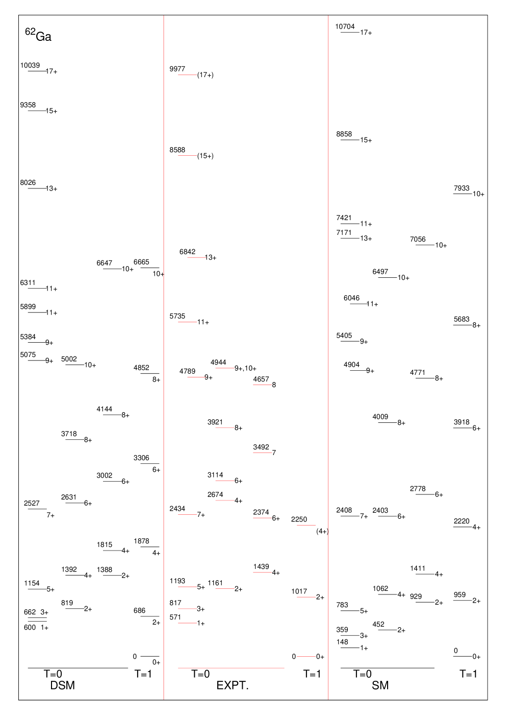
Figure 2: Comparison of deformed shell model and shell-model results using jj44b interaction with experimental data. Energies are in keV.

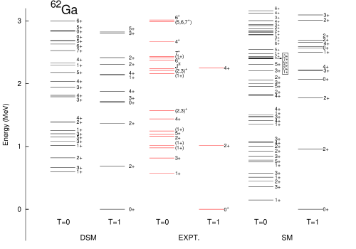
Figure 3: Comparison of experimental data david ; 62gaprl with deformed shell model and shell-model results obtained using jj44b interaction for low-lying levels up to $3$ MeV excitation. In the figure, the results for SM and DSM appear to be different and this is mainly because the energy of the lowest $T=0$ state is different in the two models. If they are aligned with the experimental level, it is seen that up to about 2 MeV excitation the two models are close to experiment.

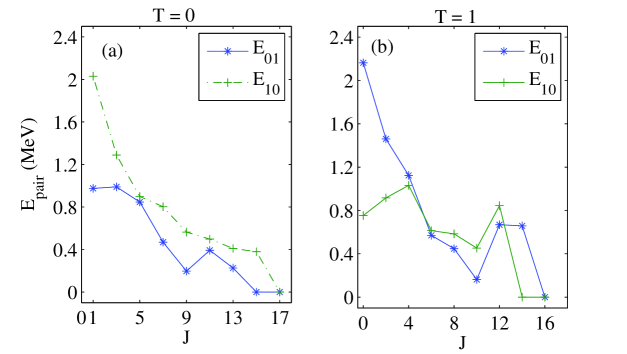
Figure 4: Pairing energies from the SM calculation for $T=0$ odd spin states and $T=1$ even spin states. Here $E_{01}$ and $E_{10}$ are isovector and isoscalar pairing, respectively.

4 Comparison with previous theoretical studies

4.1 Spectroscopy

As discussed briefly in the introduction, previous theoretical studies on ⁶²Ga using shell model, IBM-4 and Cranked Nilsson-Strutinsky model (CNS) were reported in refs. sm2 ; npa . In sm2 through a mapping, boson Hamiltonian was derived microscopically from a realistic shell model interaction. For low-lying levels one-to-one correspondence between shell model and IBM-4 was obtained. With IBM-4 the first excited 1⁺ and 3⁺ levels were correctly reproduced. Also, IBM-4 with MS interaction (ref. npa ) reproduces correctly the $T=0$ and $T=1$ band head separation. In present study, jj44b interaction predicts this separation to be 148 keV compared to the experimental value 571 keV. However the relative spacings are quite well reproduced in our study as in npa . In the previous shell model study sm2 up to 2.5 MeV only four 1⁺ ($T=0$) levels were reported while in the recent experimental work 62gaprl six plausible 1⁺ levels were reported. However, our shell model calculations with jj44b interaction generates six 1⁺ ($T=0$) levels as seen in experiment. The first 2⁺ ($T=1$) level is compressed in sm2 while our shell model results are much better with difference of only 58 keV.

The change in occupancy of the levels as we go to higher spins provide information regarding the change in structure of these levels. As seen in table 2, we find that all the $T=0$ odd spin states up to $J=11^{+}$ are predominantly from $f_{5/2}$ orbital. The occupation of $f_{5/2}$ orbital also increases with spin. However, for higher spin states the $g_{9/2}$ occupancy is about 2. As discussed before, the DSM also predicts a band crossing where a $K=1^{+}$ band obtained by excitation of two particles to $g_{9/2}$ crosses the ground band at $J=13^{+}$ and becomes yrast. Band crossing is the mechanism for back bending and both our SM and DSM reproduces this phenomenon. Similar results were also obtained by Juodagalvis and Åberg (ref. npa ) in their shell model and CNS calculations. However the transition point was at spin $J=9^{+}$ in their calculation. As seen in table 2, the occupancy of the $T=1$ even spin states are predominately from $f_{5/2}$ with occupancy of $f_{5/2}$ increasing with spin up to $J=10^{+}$. Similar trend was seen in ref. npa . The importance of inclusion of $f_{7/2}$ orbital in the shell model space is reported in ref. npa from the result of occupancy of the orbitals in Cranked Nilsson-Strutinsky model (CNS). They argued that the smaller value of $|Q_{spec}|$ in SM result (fig. 9, ref. npa ) reflects the importance of inclusion of $f_{7/2}$ orbital.

As indicated in fig. 8 ( ref. npa ), our $B(E2)$’s value are also larger for $T=1$ band compared to $T=0$ band. The shell model in ref. npa predicts $B(E2,3^{+}\rightarrow 1^{+})$ to be about 100 $e^{2}fm^{4}$. This value in the present shell model is 94. The trend for higher spins is also reasonably well reproduced. The CNS model predicts faster decrease in $B(E2)$ as one goes to higher spins. For example $B(E2,15_{1}^{+}\rightarrow 13_{1}^{+}$) and $B(E2,17_{1}^{+}\rightarrow 15_{1}^{+})$ in our calculation are 182 and 124 $e^{2}fm^{4}$. These values are larger than the values given in ref. npa . The $B(E2)$ values for $T=1$ even spin states show a slow rising trend and finally decreases for $10^{+}$ as in ref. npa .

In ref. npa it was concluded that for the low spin parts of the bands with $T=0$ and $T=1$ corresponds to triaxially deformed states with the rotation taking place around the shortest and intermediate axis, respectively. Our result also supporting this conclusion because of different values of electromagnetic properties of these two bands (see, tables 3 and 4) and also because DSM description shows mixing of several intrinsic states.

4.2 Pairing Energy

We have also calculated the pairing energy following the procedure laid down in ref. povesplb . The two body matrix elements for the isovector pairing $P01$ and isoscalar pairing $P10$ in jj coupling scheme are,

$$\begin{array}[]{l}\lx@intercol\lx@intercol\@ADDCLASS{ltx_eqn_lefteqn}$\displaystyle\left\langle j_{a}j_{b}JT|P01|j_{c}j_{d}JT\right\rangle$\mbox{}\hfil\lx@intercol\\ \\ =G\sqrt{(j_{a}+1/2)(j_{c}+1/2)}\delta_{ab}\delta_{cd}\delta_{J0}\delta_{T1}\;,\end{array}$$ (3)

$$\begin{array}[]{l}\lx@intercol\lx@intercol\@ADDCLASS{ltx_eqn_lefteqn}$\displaystyle\left\langle j_{a}j_{b}JT|P10|j_{c}j_{d}JT\right\rangle$\mbox{}\hfil\lx@intercol\\ \\ =G\frac{2(-1)^{j_{a}-j_{c}}}{\sqrt{1+\delta_{ab}}\sqrt{1+\delta_{cd}}}\\ \\ \times\sqrt{(2j_{a}+1)(2j_{b}+1)(2j_{c}+1)(2j_{d}+1)}\\ \\ \times\left\{\begin{array}[]{ccc}1/2&j_{a}&l_{a}\\ j_{b}&1/2&1\end{array}\right\}\left\{\begin{array}[]{ccc}1/2&j_{c}&l_{c}\\ j_{d}&1/2&1\end{array}\right\}\\ \\ \times\delta_{l_{a}l_{b}}\delta_{l_{c}l_{d}}\delta_{J1}\delta_{T0}\;.\end{array}$$ (4)

We have calculated the pairing energy by taking the energy difference of states calculated with the full Hamiltonian jj44b and the Hamiltonian $H_{eff}$ obtained by subtracting from jj44b Hamiltonian P01 or P10 pairing interaction. We have used $G$ = 0.276 for P01 and $G$ = 0.506 for P10 following refs. povesplb ; zuker . The contribution of pairing energies for $T=0$ odd spin states and $T=1$ even spin states are shown in the figs. 4(a) and (b). Our results are similar to the values obtained by Juodagalvis and Åberg (JA)npa . However there are some important differences. Juodagalvis and Åberg found that the $T=1$, $J=0$ ground state has equal contribution of pairing energy from $T=0$ and T=1 channels. However, we find that the two contributions are approximately equal for $J\geq 4^{+}$ for both $T=0$ (odd $J$) and $T=1$ (even $J$) levels. For the even $T=1$ levels with $J<4^{+}$, isovector pairing plays a larger role. Similarly, for $T=0$ levels with $J<5^{+}$, the isoscalar pairing plays a much greater role. JA also found a similar trend above the band crossing region. However below the band crossing region, the isoscalar pairing is much larger than the isovector pairing. They have obtained a measure of the contribution of isovector pairing mode. Due of isospin symmetry, the three parts of the isovector pairing, $nn$, $pp$ and $np$, are identical in the $T=0$ states. Their calculation shows that each component of the isovector pairing mode contributes about 0.25 MeV to the $T=0,J=1$ state and in our case it is (see fig. 4a) 0.30 MeV.

From the studies of pairing energy for $T=0$ and $T=1$ bands, Juodagalvis and Åberg have tried to understand how pairing energy plays an important role in making the $T=1$ state to become the ground state. We have made a similar analysis using our calculation. The isoscalar pairing for the lowest $T=0$ and lowest $T=1$ bands is about 2 and 0.8 MeV. Similarly the isovector pairing for the two cases are 1 and 2.3 MeV. Thus the total pairing energy for $T=0$,$J=1$ is 3 MeV whereas for $T=1$,$J=0$, the total pairing energy is 3.1 MeV. Thus our calculation also shows that the $T=1$ band should be lower compared to the $T=0$ band because of the gain of 0.1 MeV in pairing energy. It may be noted that our SM calculation with jj44b interaction predicts the $T=1$ and $T=0$ band head separation to be 148 keV compared to the experimental value 571 keV whereas the MS interaction in JA correctly reproduces the separation. Hence compared to JA, our SM with jj44b interaction shows a lesser favoring of pairing energy for $T=1$ ground state.

5 Conclusions

In the present work we have compared results of recently available experimental data for $T=0$ and $T=1$ states for ⁶²Ga within shell model and deformed shell model results obtained using jj44b interaction. As discussed in detail in Section 3, the SM and DSM explain the experimental data well. The analysis shows that DSM with much smaller number of (deformed) configurations is adequate for ⁶²Ga. The present analysis goes much beyond the analysis presented before for ⁶²Ga using SM and DSM in refs. [17,18] and adds more information. In future, it is also important to improve further the effective interactions in $f_{5/2}pg_{9/2}$ space and also include proton and neutron excitations across the $Z=28$ shell by including the $1f_{7/2}$ orbital in the model space.

Further, the following broad conclusions can be drawn:

$\bullet$ The present shell model and the deformed shell model calculations with jj44b interaction describe the spectroscopic data reasonably well.

$\bullet$ We have calculated the $B(E2)$ values for isovector and isoscalar transitions. Comparison with one experimental data available for this nucleus is good. The $B(E2)$’s for $T=1$ even spin states show a slow rising trend and finally decrease for $J=10^{+}$.

$\bullet$ Both SM and DSM with jj44b interaction showed a band crossing starting at $J=13^{+}$ for the lowest $T=0$ band (band crossing is the mechanism for back-bending). Past CSM calculations showed band crossing at $J=9^{+}$ npa .

$\bullet$ We have calculated the pairing energy for $T=0$ and $T=1$ bands. We find that for the lowest $T=0$ band, the contributions from isoscalar and isovector pairing are approximately equal for $J\geq 5^{+}$ while for $J<5^{+}$, isovector pairing plays a larger role.

$\bullet$ The present shell model results correctly predict six $1^{+}$ levels with $T=0$ as reported in a recent experiment 62gaprl .

$\bullet$ We also obtain low level density at low energy for ⁶²Ga in agreement with experiment.

$\bullet$ Future experimental investigations with radioactive ion beam facilities will be required for generating more information about the structure the $T=0$ and $T=1$ bands and the nature of $T=0$ and $T=1$ pairing in heavier $N=Z$ odd-odd nuclei.

The authors are thankful to Profs. B.A. Brown, R. Palit, David Jenkins and Dr. P. Ruotsalainen for useful discussions. RS is thankful to DST (Government of India) for financial support.

References

- (1) S.M. Fischer et al.. Phys. Rev. Lett. 84, 4064 (2000).
- (2) G. de Angelis et al., Phys. Lett. B 415, 217 (1997).
- (3) C.J. Lister et al., Phys. Rev. C 42, R1191 (1990).
- (4) C.J. Lister et al., Phys. Rev. Lett. 59, 1270 (1987).
- (5) W. Gelletly et al., Phys. Lett. B 253, 287 (1991).
- (6) N. Marginean et al., Phys. Rev. C 63, 031303(R) (2001).
- (7) S.M. Vincent et al., Phys. Lett. B 437, 264 (1998).
- (8) D. Rudolph et al., Phys. Rev. C 69, 034309 (2004).
- (9) H.M. David et al., Phys. Lett. B 726, 665 (2013).
- (10) P. Ruotsalainen et al., Phys. Rev. C 88, 024320 (20013).
- (11) D.G. Jenkins et al.. Phys. Rev. C 65, 064307 (2002).
- (12) D. Rudolph et al., Phys. Rev. Lett. 76, 376 (1996).
- (13) C.D. O’Leary et al., Phys. Rev. C 67, 021301(R) (2003).
- (14) S.M. Fischer et al.. Phys. Rev. C 74, 054304 (2006).
- (15) B.S. Nara Singh et al., Phys. Rev. C 75, 061301(R) (2007).
- (16) E. Grodner et al., Phys.Rev.Lett. 113, 092501 (2014).
- (17) O. Juillet, P. Van Isacker, D.D. Warner, Phys. Rev. C 63, 054312 (2001).
- (18) R. Sahu and V.K.B. Kota, Phys. Rev. C 66, 024301 (2002).
- (19) E. Caurier, F. Nowacki, A. Poves, J. Retamosa, Phys. Rev. Lett. 77, 1954 (1996).
- (20) B.A. Brown and A.F. Lisetskiy (unpublished); see also endnote (28) in B. Cheal et al., Phys. Rev. Lett. 104, 252502 (2010).
- (21) A. Juodagalvis and S. Åberg, Nucl. Phys. A 683, 207 (2001).
- (22) B.A. Brown et al. NuShell@MSU.
- (23) R. Sahu, P.C. Srivastava and V.K.B. Kota, J. Phys. G 40, 095107 (2013).
- (24) R. Sahu and V.K.B. Kota, Phys. Rev. C 66, 024301 (2002).
- (25) R. Sahu and V.K.B. Kota, Phys. Rev. C 67, 054323 (2003).
- (26) S. Mishra, R. Sahu, and V.K.B. Kota, Prog. Theo. Phys. 118, 59 (2007).
- (27) A. Poves and G. Martinez-Pinedo, Phys. Lett. B 430, 203 (1998).
- (28) M. Dufour and A.P. Zuker, Phys. Rev. C 54, 1641 (1996).