Seasonality effects on Dengue: basic reproduction number,
sensitivity analysis and optimal control

Abstract

Dengue is a vector-borne disease transmitted from an infected human to an Aedes mosquito, during a blood meal. Dengue is still a major public health problem. A model for the disease transmission is presented, composed by human and mosquitoes compartments. The aim is to simulate the effects of seasonality, on the vectorial capacity and, consequently, on the disease development. Using entomological information about the mosquito behavior under different temperatures and rainfall, simulations are carried out and the repercussions analyzed. The basic reproduction number of the model is given, as well as a sensitivity analysis of model’s parameters. Finally, an optimal control problem is proposed and solved, illustrating the difficulty of making a trade-off between reduction of infected individuals and costs with insecticide.

Keywords: dengue; vectorial capacity; seasonality; basic reproduction number; sensitivity analysis; optimal control.

2010 Mathematics Subject Classification: 34A34; 49J15; 49K15; 92B05.

1 Introduction

Dengue is currently one of the most important viral diseases transmitted by mosquitoes to humans in a world context. It is transmitted by Aedes aegypti and Aedes albopictus and is usually found in tropical and sub-tropical regions, but some recent episodes also happened in Europe [11, 24, 26]. There are four different serotypes that can cause dengue fever. A human infected by one serotype, when recovered, has total immunity for that one, and only has partial and transient immunity for the other three serotypes.

The life cycle of the mosquito has four distinct stages: egg, larva, pupa and adult. The first three stages take place in water, while air is the medium for the adult stage. In urban areas, Aedes aegypti breeds on water collections. With increasing urbanization and crowded cities, environmental conditions foster the spread of the disease that, even in the absence of fatal forms, breed significant economic and social costs (absenteeism, immobilization, debilitation and medication) [6]. Until a vaccine or drug for dengue is available, vector control operations that eliminate adult mosquitoes and their larvae through breeding-source reduction remain the only effective method [30]. However, vector control can be expensive and time consuming, producing a huge economic burden on nations.

Dengue epidemiology is influenced by a complex set of factors that include rapid urbanization and increase in population density, capacity of healthcare systems, herd immunity and social behavior of the population. However, temperature and rainfall are a key environmental determinant in shaping the landscape of disease. They are critical to mosquito survival, reproduction and development, and can influence mosquito presence and abundance [2]. Additionally, higher temperatures reduce the time required for the virus to replicate and disseminate in the mosquito [15, 17, 28]. Thus, it is important to create distinct simulations to predict the effects of seasonality on the disease transmission.

The text is organized as follows. In Section 2, a mathematical model of the interaction between humans and mosquitoes is formulated, and the basic reproduction number, $\mathcal{R}_{0}$, is calculated. A sensitivity analysis of the parameters used is carried out taking into account $\mathcal{R}_{0}$. Different simulations of the model are shown, varying the temperatures of the region. In Section 3, the mathematical model is restructured, using a periodic function for the birthrate of the mosquito, fitting a region with dry and rainy seasons all over a year. An optimal control problem is proposed in Section 4, using the information given in Section 2, in order to analyze different bioeconomic approaches for the dengue disease. The main conclusions are given in Section 5.

2 The mathematical model

Taking into account the model presented in [7, 8] and the considerations of [20, 21, 23], a mathematical model is here proposed. It includes three epidemiological states for humans:

$S_{h}(t)$	—	susceptible (individuals who can contract the disease);
$I_{h}(t)$	—	infected (individuals who can transmit the disease); and
$R_{h}(t)$	—	resistant (individuals who have been infected and have recovered).

These compartments are mutually exclusive. There are two other state variables, related to the female mosquitoes (male mosquitos are not considered because they do not bite humans and consequently do not influence the dynamics of the disease):

$S_{m}(t)$	—	susceptible (mosquitoes that can contract the disease); and
$I_{m}(t)$	—	infected (mosquitoes that can transmit the disease).

In order to make a trade-off between simplicity and reality of the epidemiological model, some assumptions are considered:

• there is no vertical transmission, that is, an infected mosquito cannot transmit the disease to their eggs;

• total human population $N_{h}$ is constant: $S_{h}(t)+I_{h}(t)+R_{h}(t)=N_{h}$ at any time $t$;

• the mosquito population is also constant and proportional to human population, that is, $S_{m}(t)+I_{m}(t)=N_{m}$, with $N_{m}=\kappa N_{h}$ for some constant $\kappa$;

• the population is homogeneous, which means that every individual of a compartment is homogeneously mixed with the other individuals;

• immigration and emigration are not considered during the period under study;

• homogeneity between host and vector populations, that is, each vector has an equal probability to bite any host;

• humans and mosquitoes are assumed to be born susceptible.

The system of differential equations is composed by human compartments

$$\begin{cases}\frac{dS_{h}(t)}{dt}=\mu_{h}N_{h}-\left(B\beta_{mh}\frac{I_{m}(t)}{N_{h}}+\mu_{h}\right)S_{h}(t)\\ \displaystyle\frac{dI_{h}(t)}{dt}=B\beta_{mh}\frac{I_{m}(t)}{N_{h}}S_{h}(t)-(\eta_{h}+\mu_{h})I_{h}(t)\\ \displaystyle\frac{dR_{h}(t)}{dt}=\eta_{h}I_{h}(t)-\mu_{h}R_{h}(t)\end{cases}$$ (1)

coupled with mosquito compartments

$$\begin{cases}\frac{dS_{m}(t)}{dt}=\mu_{m}N_{m}-\left(B\beta_{hm}\frac{I_{h}(t)}{N_{h}}+\mu_{m}\right)S_{m}(t)\\ \displaystyle\frac{dI_{m}(t)}{dt}=B\beta_{hm}\frac{I_{h}(t)}{N_{h}}S_{m}(t)-\mu_{m}I_{m}(t)\end{cases}$$ (2)

and subject to initial conditions

$$\begin{gathered}S_{h}(0)=S_{h0},\quad I_{h}(0)=I_{h0},\quad R_{h}(0)=R_{h0},\\ S_{m}(0)=S_{m0},\quad I_{m}(0)=I_{m0}.\end{gathered}$$ (3)

2.1 Scenarios with temperature variation

The dengue epidemic model makes use of the parameters described in Table 1. In this study, three simulations were considered, related to distinct vectorial capacity. Temperature affects the behavior of vector: its population, biting rate, biting capacity, incubation time, daily survival probability or mortality rate, and eggs hatching rate [29]. It is generally assumed that higher mean temperatures facilitate dengue transmission because of faster virus propagation and dissemination within the vector. Vector competence, the probability of a mosquito becoming infected and subsequently transmitting virus after ingestion of an infectious blood meal, is generally positively associated with temperature [1]. We only assume differences on transmission capacities and mosquito lifespan.

The different values presented for Scenarios 1 and 2 are based on [17]. The first scenario is concerned with a region where the mean temperature is $14^{\circ}$C. The second one is related to a region where the mean temperature is $26^{\circ}$C. The third scenario is created to simulate mild climate. The authors had previously analyzed the outbreak that occurred in Madeira island in October 2012, which has a mean temperature between $18^{\circ}$C and $24^{\circ}$C, all over the year. The values used in this last scenario are based on [23].

Table 1: Parameters in the epidemiological model (1)–(2).

Para-	Description	Range of values	Value	Value	Value	Source
meter		in literature	Scenario 1	Scenario 2	Scenario 3
$N_{h}$	Total population		112000	112000	112000	[14]
$N_{m}$	Total mosquito population		$3\times N_{h}$	$3\times N_{h}$	$3\times N_{h}$	[14]
$B$	Average daily biting (per day)		1/3	1/3	1/3	[9]
$\beta_{mh}$	Transmission probability
	from $I_{m}$ (per bite)	[0.1, 1]	0.12	0.99	0.2	[9, 17]
$\beta_{hm}$	Transmission probability
	from $I_{h}$ (per bite)	[0.1, 1]	0.11	0.95	0.2	[9, 17]
$1/\mu_{h}$	Average lifespan of humans
	(in days)		$\frac{1}{79\times 365}$	$\frac{1}{79\times 365}$	$\frac{1}{79\times 365}$	[14]
$1/\eta_{h}$	Average viremic period (in days)	[1/15, 1/4]	1/7	1/7	1/7	[4]
$1/\mu_{m}$	Average lifespan of adult
	mosquitoes (in days)	[1/45, 1/8]	0.04	0.03	1/15	[10, 12, 17, 18]

2.2 Stability and sensitivity analysis

The model (1)–(2) has two nonnegative equilibria. Namely,

• a disease-free equilibrium $(S_{h1},I_{h1},R_{h1},S_{m1},I_{m1})=(N_{h},0,0,N_{m},0)$;

• an endemic equilibrium $(S_{h2},I_{h2},R_{h2},S_{m2},I_{m2})$ with

  $$\begin{split}S_{h2}&=\frac{N_{h}^{2}(B\beta_{hm}\mu_{h}+\mu_{m}(\eta_{h}+\mu_{h}))}{B\beta_{hm}(B\beta_{mh}N_{m}+\mu_{h}N_{h})},\\ I_{h2}&=-\frac{\mu_{h}N_{h}\left(\mu_{m}N_{h}(\eta_{h}+\mu_{h})-B^{2}\beta_{hm}\beta_{mh}N_{m}\right)}{B\beta_{hm}(\eta_{h}+\mu_{h})(B\beta_{mh}N_{m}+\mu_{h}N_{h})},\\ R_{h2}&=-\frac{\eta_{h}N_{h}\left(\mu_{m}N_{h}(\eta_{h}+\mu_{h})-B^{2}\beta_{hm}\beta_{mh}N_{m}\right)}{B\beta_{hm}(\eta_{h}+\mu_{h})(B\beta_{mh}N_{m}+\mu_{h}N_{h})},\\ S_{m2}&=\frac{\mu_{m}(\eta_{h}+\mu_{h})(B\beta_{mh}N_{m}+\mu_{h}N_{h})}{B\beta_{mh}(B\beta_{hm}\mu_{h}+\mu_{m}(\eta_{h}+\mu_{h}))},\\ I_{m2}&=-\frac{\mu_{h}\left(\mu_{m}N_{h}(\eta_{h}+\mu_{h})-B^{2}\beta_{hm}\beta_{mh}N_{m}\right)}{B\beta_{mh}(B\beta_{hm}\mu_{h}+\mu_{m}(\eta_{h}+\mu_{h}))}.\end{split}$$

An important measure of transmissibility of the disease is given by the basic reproduction number. It represents the expected number of secondary cases produced in a completed susceptible population, by a typical infected individual during its entire period of infectiousness [13].

Theorem 1.

The basic reproduction number $\mathcal{R}_{0}$ associated to the differential system (1)–(2) is given by

$$\mathcal{R}_{0}=\left(\frac{B^{2}\beta_{hm}\beta_{mh}N_{m}}{(\eta_{h}+\mu_{h})\mu_{m}N_{h}}\right)^{\frac{1}{2}}.$$ (4)

Proof.

Similar to the one found in [22]. ∎

If $\mathcal{R}_{0}<1$, then, on average, an infected individual produces less than one new infected individual over the course of its infectious period, and the disease cannot grow. Conversely, if $\mathcal{R}_{0}>1$, then each individual infects more than one person, and the disease invades the population. Mathematically, $\mathcal{R}_{0}$ is a threshold for stability of a disease-free equilibrium and is related to the peak and final size of an epidemic [27]. If $\mathcal{R}_{0}<1$, then the disease-free equilibrium is stable; otherwise, if $\mathcal{R}_{0}>1$, then it is unstable.

In determining how best to reduce human mortality and morbidity due to dengue, it is necessary to know the relative importance of the different factors responsible for its transmission. The sensitivity indices of $\mathcal{R}_{0}$, related to the parameters in the model, are now calculated.

Sensitivity indices allow us to measure the relative change in a variable when a parameter changes. The normalized forward sensitivity index of a variable with respect to a parameter is the ratio of the relative change in the variable to the relative change in the parameter. When the variable is a differentiable function of the parameter, the sensitivity index may be defined as follows.

Definition 2 (See [5]).

The normalized forward sensitivity index of $\mathcal{R}_{0}$, which depends differentiably on a parameter $p$, is defined by

$$\Upsilon_{p}^{\mathcal{R}_{0}}=\frac{\partial\mathcal{R}_{0}}{\partial p}\times\frac{p}{\mathcal{R}_{0}}.$$ (5)

Given the explicit formula (4) for the basic reproduction number, one can easily derive an analytical expression for the sensitivity of $\mathcal{R}_{0}$ with respect to each parameter that comprise it. The obtained values are in Table 2, which presents the sensitivity indices for the baseline parameter values. Note that the sensitivity index (column 2 of Table 2) may be a complex expression, depending on the different parameters of the system, but can also be a constant value, not depending on any parameter value. Column 3 of Table 2 presents the values of the indices, considering the parameter values of Table 1.

Table 2: Sensitivity indices (5) of (4) evaluated at the baseline parameter values in Table 1.

Parameter	Sensitivity index	Sensitivity index
		for parameter values
$B$	+1	+1
$\beta_{mh}$	+0.5	+0.5
$\beta_{hm}$	+0.5	+0.5
$\mu_{h}$	$-\frac{\eta_{h}}{2(\eta_{h}+\mu_{h})}$	-0.00012
$\eta_{h}$	$-\frac{\mu_{h}}{2(\eta_{h}+\mu_{h})}$	-0.49988
$\mu_{m}$	-0.5	-0.5

For example, $\Upsilon_{\beta_{mh}}^{\mathcal{R}_{0}}\equiv+0.5$ means that increasing (or decreasing) $\beta_{mh}$ by $10\%$ increases (or decreases) always $\mathcal{R}_{0}$ by $5\%$. A highly sensitive parameter should be carefully estimated, because a small variation in that parameter will lead to large quantitative changes. An insensitive parameter, on the other hand, does not require as much effort to estimate, because a small variation in that parameter will not produce large changes to the quantity of interest. The results show that big changes in the parameters that affects the basic reproduction number (except $\mu_{h}$) produce significant changes in $\mathcal{R}_{0}$, and consequently, in the behavior of the disease development. For the three scenarios we study, the basic reproduction number has the values 0.7698, 73.1322 and 0.6221, respectively. This means that if there is no change or control for the disease, the outbreak will die out in a short period in Scenarios 1 and 3. In contrast, the disease will persist and will become endemic in the region of Scenario 2.

2.3 Numerical analysis

The software used in our simulations was Matlab with the routine ode45. This solver is based on an explicit Runge–Kutta (4,5) formula, the Dormand–Prince pair. That means the numerical solver ode45 combines fourth and fifth order methods, both of which are similar to the classical fourth order Runge–Kutta method. These vary the step size, choosing it at each step in an attempt to achieve the desired accuracy. We examine simulations of system (1)–(2), considering final time $t_{f}=365$ days with the following initial values (3) for the differential equations:

$$\begin{gathered}S_{h}(0)=111991,\quad I_{h}(0)=9,\quad R_{h}(0)=0,\\ S_{m}(0)=335000,\quad I_{m}(0)=1000.\end{gathered}$$

Figure 1 shows the evolution of infected human in the three scenarios, respectively. Figure 1(b) presents more infected people, because it corresponds to higher levels of disease transmissibility due to higher temperatures. Besides, it is also this scenario that reaches the peak of the disease faster, while the third simulation has its higher transmission after 200 days. A situation like this last one allows to have time to prepare the fight of the disease, in terms of control measures and medical surveillance.

Besides the constraint of temperature effects, the rainfall factor is also included in next section.

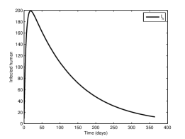
(a) Scenario 1

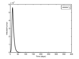
(b) Scenario 2

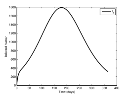
(c) Scenario 3

Figure 1: Infected human.

3 Mathematical model with seasonal variation of mosquito

In this section, we study the effect of rainfall on the pattern of mosquito reproduction and hence the number of mosquitoes. We maintain all the assumptions given before, except assuming that birth and death rates are equal over time. The seasonal effect in the modeling of virus transmission is incorporated, allowing the total number of mosquitoes to vary periodically with time.

Following [15], we include this seasonal pattern in system (1)–(2) by changing the birthrate of mosquitoes to a periodic function

$$\mu_{m}\left(1+\alpha\cos\left(\frac{2\pi t}{365}\right)\right),$$

where $\mu_{m}$ is the per capita death rate of mosquitoes and $\alpha$ is the amplitude of the seasonal variation, with $0<\alpha<1$. So, the differential equation in (2) related to the susceptible mosquitos is transformed into

$$\frac{dS_{m}(t)}{dt}=\mu_{m}\left(1+\alpha\cos\left(\frac{2\pi t}{365}\right)\right)\left(S_{m}(t)+I_{m}(t)\right)-\left(B\beta_{hm}\frac{I_{h}(t)}{N_{h}}+\mu_{m}\right)S_{m}(t).$$

This reformulated model has only the trivial equilibrium $(\tilde{S}_{h1},\tilde{I}_{h1},\tilde{R}_{h1},\tilde{S}_{m1},\tilde{I}_{m1})=(N_{h},0,0,0,0)$.

For numerical experiments, we considered $\alpha=0.3$. In this way, the mosquito reproduction has its lowest value around 190 days after the beginning of the year. Again, the routine ode45 of Matlab was used. Figure 2 presents the simulations. The solid line shows the situation described in Section 2.3 with all the parameters fixed; in dashed line, we represent the simulation with the periodic function. In all situations, the simulations with the seasonal pattern present more infected people. In Scenario 1, the peak of the disease with the periodic function is reached later, while in Scenario 3, the situation is reversed.

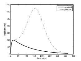
(a) Scenario 1

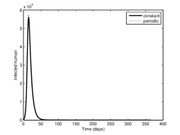
(b) Scenario 2

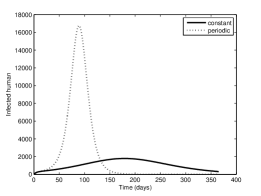
(c) Scenario 3

Figure 2: Infected human using a constant and a periodic mosquito population (solid and dashed lines, respectively).

With the aim of fighting the disease, reducing simultaneously the costs with infected individuals and the costs of insecticide campaigns to kill the mosquito, an optimal control problem is presented and analysed in the next section.

4 Optimal control problem

The control strategies for the reduction of infected individuals imply a cost of implementation. This cost can be modeled through the formulation of an optimal control problem, mathematically traduced by adding a functional.

Let us consider the previous differential system (1)–(2) with constant mosquito population. To this, we add to the mosquito compartments the control insecticide, $u(t)$, with $0\leq u(t)\leq 1$. Thus, the second part of the differential system is rewritten as

$$\begin{cases}\frac{dS_{m}(t)}{dt}=\mu_{m}N_{m}-\left(B\beta_{hm}\frac{I_{h}(t)}{N_{h}}+\mu_{m}+u(t)\right)S_{m}(t),\\ \frac{dI_{m}(t)}{dt}=B\beta_{hm}\frac{I_{h}(t)}{N_{h}}S_{m}(t)-\left(\mu_{m}+u(t)\right)I_{m}(t).\end{cases}$$ (6)

Our aim is to minimize the number of infected individuals, $I_{h}$, while keeping the cost of control strategy implementation low, that is, we want to minimize

$$C\left(u\right)=\int_{0}^{t_{f}}\left[\gamma_{D}I_{h}(t)+\gamma_{S}u^{2}(t)\right]dt,$$ (7)

where the coefficients $\gamma_{D}$ and $\gamma_{S}$ represent the balancing cost factors for infected individuals and spraying campaigns, respectively. More precisely, the optimal control problem consists in finding a control $u^{*}$ such that the associated state trajectory $\left(S_{h}^{*},I_{h}^{*},R_{h}^{*},S_{m}^{*},I_{m}^{*}\right)$ is solution of the control system (1) and (6) in the interval $[0,t_{f}]$ with the initial conditions (3) and minimizing the cost functional $C$:

$$C(u^{*})=\min_{u\in\Omega}C(u),$$ (8)

where $\Omega$ is the set of admissible controls given by $\Omega=\{u\in L^{1}(0,t_{f})\,|\,0\leq u(t)\leq 1\}$. The existence of the optimal control $u^{*}(\cdot)\in\Omega$ comes from the convexity of the cost functional (7) with respect to the control and the regularity of the system (1) and (6) (see, e.g., [3] for existence results of optimal solutions). According to the Pontryagin minimum principle [19], if $u^{*}(\cdot)$ is optimal for the problem (8), (1) and (6) with the initial conditions given by (3) and fixed final time $t_{f}$, then there exists an adjoint vector, $\lambda=\left(\lambda_{1}(t),\lambda_{2}(t),\lambda_{3}(t),\lambda_{4}(t),\lambda_{5}(t)\right)$, such that

$$\dot{S}_{h}=\frac{\partial H}{\partial\lambda_{1}},\quad\dot{I}_{h}=\frac{\partial H}{\partial\lambda_{2}},\quad\dot{R}_{h}=\frac{\partial H}{\partial\lambda_{3}},\quad\dot{S}_{m}=\frac{\partial H}{\partial\lambda_{4}},\quad\dot{I}_{m}=\frac{\partial H}{\partial\lambda_{5}}$$

and

$$\dot{\lambda}_{1}=-\frac{\partial H}{\partial S_{h}},\quad\dot{\lambda}_{2}=-\frac{\partial H}{\partial I_{h}},\quad\dot{\lambda}_{3}=-\frac{\partial H}{\partial R_{h}},\quad\dot{\lambda}_{4}=-\frac{\partial H}{\partial S_{m}},\quad\dot{\lambda}_{5}=-\frac{\partial H}{\partial I_{m}},$$

where function $H$, called the Hamiltonian, is defined by

$$\begin{split}H=&\gamma_{D}I_{h}+\gamma_{S}u^{2}\\ &+\lambda_{1}\left(\mu_{h}N_{h}-\left(B\beta_{mh}\frac{I_{m}}{N_{h}}+\mu_{h}\right)S_{h}\right)\\ &+\lambda_{2}\left(B\beta_{mh}\frac{I_{m}}{N_{h}}S_{h}-(\eta_{h}+\mu_{h})I_{h}\right)\\ &+\lambda_{3}\left(\eta_{h}I_{h}-\mu_{h}R_{h}\right)\\ &+\lambda_{4}\left(\mu_{m}N_{m}-\left(B\beta_{hm}\frac{I_{h}}{N_{h}}+\mu_{m}\right)S_{m}\right)\\ &+\lambda_{5}\left(B\beta_{hm}\frac{I_{h}}{N_{h}}S_{m}-\mu_{m}I_{m}\right).\end{split}$$

Moreover, the minimality condition

$$H\left(S_{h}^{*}(t),I_{h}^{*}(t),R_{h}^{*}(t),S_{m}^{*}(t),I_{m}^{*}(t),\lambda(t),u^{*}(t)\right)\\ =\min_{0\leq u\leq 1}H\left(S_{h}^{*}(t),I_{h}^{*}(t),R_{h}^{*}(t),S_{m}^{*}(t),I_{m}^{*}(t),\lambda(t),u\right)$$

holds almost everywhere on $[0,t_{f}]$ together with the transversality conditions

$$\lambda_{i}(t_{f})=0,\quad i=1,\ldots,5.$$

Theorem 3.

The optimal control problem (8), (1), (6) with fixed initial conditions (3) and fixed final time $t_{f}$ admits an unique solution $\left(S_{h}^{*},I_{h}^{*},R_{h}^{*},S_{m}^{*},I_{m}^{*}\right)$ associated to an optimal control $u^{*}(\cdot)$ on $[0,t_{f}]$. Moreover, there exists adjoint functions $\lambda_{1}^{*}(\cdot)$, $\lambda_{2}^{*}(\cdot)$, $\lambda_{3}^{*}(\cdot)$, $\lambda_{4}^{*}(\cdot)$ and $\lambda_{5}^{*}(\cdot)$ such that

$$\begin{cases}\dot{\lambda}_{1}^{*}(t)=(\lambda_{1}^{*}(t)-\lambda_{2}^{*}(t))B\beta_{mh}I_{m}^{*}(t)+\lambda_{1}^{*}(t)\mu_{m}\\ \dot{\lambda}_{2}^{*}(t)=(\lambda_{4}^{*}(t)-\lambda_{5}^{*}(t))B\beta_{hm}I_{h}^{*}(t)+\lambda_{2}^{*}(t)(\eta_{h}+\mu_{h})\\ \dot{\lambda}_{3}^{*}(t)=\lambda_{3}^{*}(t)\mu_{h}\\ \dot{\lambda}_{4}^{*}(t)=(\lambda_{4}^{*}(t)-\lambda_{5}^{*}(t))B\beta_{hm}I_{h}^{*}(t)+\lambda_{4}^{*}(t)(\mu_{m}+u^{*}(t))\\ \dot{\lambda}_{5}^{*}(t)=(\lambda_{1}^{*}(t)-\lambda_{2}^{*}(t))B\beta_{mh}S_{h}^{*}(t)+\lambda_{5}^{*}(\mu_{m}+u^{*}(t))\end{cases}$$ (9)

with transversality conditions

$$\lambda_{i}^{*}(t_{f})=0,\quad i=1,\ldots 5.$$ (10)

Furthermore,

$$u^{*}(t)=\min\left\{\max\left\{0,\frac{\lambda_{4}^{*}(t)S_{m}^{*}(t)+\lambda_{5}^{*}(t)I_{m}^{*}(t)}{2\gamma_{S}}\right\},1\right\}.$$ (11)

Proof.

Similar to the one found in [25]. ∎

For the optimal control problem, we used the parameter values of Scenario 2, because it is the case more threatening for public health and, therefore, the one that all efforts must be invested. For the first two graphics (Figures 3 and 4), both balancing costs, $\gamma_{D}$ and $\gamma_{S}$, assume the value one. The problem was solved in Matlab, using the forward-backward sweep method [16]. The process begins with an initial guess on the control variable. Then, the state equations are simultaneously solved forward in time and the adjoint equations are solved backward in time. The control is updated by inserting the new values of states and adjoints into its characterization, and the process is repeated until convergence occurs.

We start showing that the implementation of the control has a positive impact on the reduction of infected individuals. Figure 3 reports that the fraction of infected individuals significantly decreases when control strategies are implemented. More precisely, with the control strategy, the infected people is near to zero after 150 days, whereas without control the outbreak lasts more than one year. To minimize the total number of infectious, the optimal control $u^{*}$ is applied, which decreases to the lower bound at the end of the year (see Figure 4).

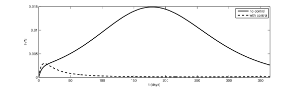
Figure 3: Fraction of infected individuals $I_{h}/N_{h}$ with and without control, where $\gamma_{D}=\gamma_{S}=1$.

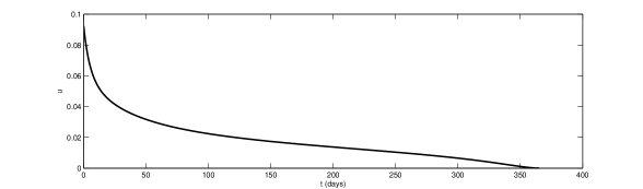
Figure 4: Optimal control $u^{*}$ with $\gamma_{D}=\gamma_{S}=1$.

The relevance of the optimal control strategies were tested, in the reduction of the fraction of infected individuals $I_{h}/N_{h}$ (Figures 5 and 6). Three bioeconomic approaches were simulated: the first one where both human and economic factors are considered ($\gamma_{D}=\gamma_{S}=1$); the second one where the human factor is preponderant ($\gamma_{D}=1$ and $\gamma_{S}=0$); and the last one, where the main issue is the economic costs with insecticide ($\gamma_{D}=0$ and $\gamma_{S}=1$). As expected, the higher values for infected individuals are reached in the third bioeconomic approach. The same approach, presents the optimal curve for $u$ close to zero, because it is expensive to apply insecticide.

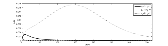
Figure 5: Fraction of infected individuals $I_{h}/N_{h}$ with distinct bioeconomic approaches.

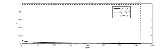
Figure 6: Optimal control $u^{*}$ with distinct bioeconomic approaches.

5 Conclusion

Temperature and rainfall can be either an effective barrier or a facilitator of vector-borne diseases. The ambient temperature increased over the last few decades, and may contribute to the drastic increase of dengue cases. In this paper, we showed that small changes in the parameters of the model, related to vectorial competence, can provoke great changes in the study of dengue disease. In most regions where the disease is present, there is at least two seasons, with distinct temperature and humidity. In this way, a periodic function that allows to fit the mosquito population along the year can be an interesting tool to the design of mathematical models.

Epidemiological modeling has largely focused on identifying the mechanisms responsible for epidemics but has taken little account on economic constraints in analyzing control strategies. Economic models have given insight into optimal control under constraints imposed by limited resources, but they frequently ignore the spatial and temporal dynamics of the disease. Nowadays, the combination of epidemiological and economic factors is essential. Therefore, we varied the cost functional, giving a different answer depending on the main goal to reach, thinking in economical or human-centered perspectives.

References

- [1] L. B. Carrington, M. V. Armijos, L. Lambrechts and T. W. Scott, Fluctuations at a low mean temperature accelerate dengue virus transmission by Aedes aegypti, PLoS Negl Trop Dis 7(4): e2190, 2013.
- [2] Centers for Disease Control and Prevention (CDC), Division of Vector Borne and Infectious Diseases, Prevention: How to reduce your risk of dengue infection, 2010.
- [3] L. Cesari, Optimization – Theory and Applications. Problems with Ordinary Differential Equations, Applications of Mathematics 17, Springer-Verlag, New York, 1983.
- [4] M. Chan and M. A. Johansson, The incubation periods of dengue viruses, PLoS ONE, 7(11):e50972, 2012.
- [5] N. Chitnis, J. Hyman and J. M. Cusching, Determining important parameters in the spread of malaria through the sensitivity analysis of a mathematical model, Bulletin of Mathematical Biology, 70(5):1272–1296, 2008.
- [6] M. Derouich and A. Boutayeb, Dengue fever: Mathematical modelling and computer simulation, Appl. Math. Comput., 177(2):528–544, 2006.
- [7] Y. Dumont and F. Chiroleu, Vector control for the chikungunya disease, Mathematical Bioscience and Engineering, 7(2):313–345, 2010.
- [8] Y. Dumont, F. Chiroleu and C. Domerg, On a temporal model for the chikungunya disease: modeling, theory and numerics, Math. Biosci., 213(1):80–91, 2008.
- [9] D. A. Focks, R. J. Brenner, J. Hayes and E. Daniels, Transmission thresholds for dengue in terms of Aedes aegypti pupae per person with discussion of their utility in source reduction efforts, Am. J. Trop. Med. Hyg., 62:11–18, 2000.
- [10] D. A. Focks, D. G. Haile, E. Daniels and G. A. Mount, Dynamic life table model for Aedes aegypti (Diptera: Culicidae): analysis of the literature and model development, J. Med. Entomol., 30:1003–1017, 1993.
- [11] I. Gjenero-Margan et al., Autochthonous dengue fever in Croatia, August-September 2010, Euro Surveill. 16(9):1–4, 2011.
- [12] L. C. Harrington et al., Analysis of survival of young and old Aedes aegypti (Diptera: Culicidae) from Puerto Rico and Thailand, Journal of Medical Entomology, 38:537–547, 2001.
- [13] H. W. Hethcote, The mathematics of infectious diseases, SIAM Rev., 42(4):599–653, 2000.
- [14] INE, Statistics of Portugal, http://censos.ine.pt
- [15] A. James, Coexistence of two serotypes of dengue virus with and without seasonal variation, Tecnical Report, 2013.
- [16] S. Lenhart and J. T. Workman, Optimal control applied to biological models, Chapman & Hall/CRC Mathematical and Computational Biology Series, Chapman & Hall/CRC, Boca Raton, FL, 2007.
- [17] J. Liu-Helmersson, H. Stenlund, A. Wilder-Smith and J. Rocklöv, Vectorial capacity of Aedes aegypti: Effects of temperature and implications for global dengue epidemic potential, PLoS ONE 9(3): e89783, 2014.
- [18] R. Maciel-de-Freitas, W. A. Marques, R. C. Peres, S. P. Cunha and R. Lourenço-de-Oliveira, Variation in Aedes aegypti (Diptera: Culicidae) container productivity in a slum and a suburban district of Rio de Janeiro during dry and wet seasons, Mem. Inst. Oswaldo Cruz, 102:489–496, 2007.
- [19] L. S Pontryagin, V. G. Boltyanskii, R. V. Gamkrelidze and E. F. Mishchenko, The mathematical theory of optimal processes, Translated from the Russian by K. N. Trirogoff, Interscience Publishers John Wiley & Sons, Inc., New York-London, 1962.
- [20] H. S. Rodrigues, M. T. T. Monteiro and D. F. M. Torres, Optimization of dengue epidemics: a test case with different discretization schemes, AIP Conf. Proc., 1168(1):1385–1388, 2009. arXiv:1001.3303
- [21] H. S. Rodrigues, M. T. T. Monteiro and D. F. M. Torres, Insecticide control in a dengue epidemics model, AIP Conf. Proc., 1281(1):979–982, 2010. arXiv:1007.5159
- [22] H. S. Rodrigues, M. T. T. Monteiro and D. F. M. Torres, Vaccination models and optimal control strategies to dengue, Math. Biosci., 247(1):1–12, 2014. arXiv:1310.4387
- [23] H. S. Rodrigues, M. T. T. Monteiro, D. F. M. Torres, A. C. Silva, C. Sousa and C. Conceição, Dengue in Madeira island, Mathematics of Planet Earth, CIM Mathematical Sciences, Springer, in press. arXiv:1409.7915
- [24] G. La Ruche et al., First two autochthonous dengue virus infections in metropolitan France, September 2010, Euro Surveill. 15(39): 1–5, 2010.
- [25] C. J. Silva and D. F. M. Torres, Optimal control strategies for tuberculosis treatment: a case study in Angola, Numer. Algebra Control Optim., 2(3): 601–617, 2012. arXiv:1203.3255
- [26] C. A. Sousa et al., Ongoing outbreak of dengue type 1 in the Autonomous Region of Madeira, Portugal: preliminary report, Euro Surveill 17(49): 1–4, 2012.
- [27] P. van den Driessche and J. Watmough, Reproduction numbers and sub-threshold endemic equilibria for compartmental models of disease transmission, Math. Biosci., 180: 29–48, 2002.
- [28] D. Vezzani, S. M. Vel squez and N. Schweigmann, Seasonal Patter of Abundance of Aedes aegypti (Diptera: Culicidae) in Buenos Aires City, Argentina, Mem. Inst. Oswaldo Cruz, Rio de Janeiro, 99(4): 351–356, 2004.
- [29] D. M. Watts, D. S. Burke, B. A. Harrison, R. E. Whitmire and A. Nisalak, Effect temperature on the vector efficiency of Aedes aegypti for dengue 2 virus, Am. J. Trop. Hyg. 36(1):143–152, 1987.
- [30] WHO. Dengue: guidelines for diagnosis, treatment, prevention and control, World Health Organization, 2nd edition, Geneva, 2009.