The time delay in strong gravitational lensing with Gauss-Bonnet correction

Abstract

The time delay between two relativistic images in the strong gravitational lensing governed by Gauss-Bonnet gravity is studied. We derive and calculate the expression of time delay due to the Gauss-Bonnet coupling. It is shown that the time delay for two images with larger space each other is longer. We also find that the ratio of Gauss-Bonnet coefficient and the mass of gravitational source changes in the region like $\frac{\alpha}{M}\in[0,2)$. The time delay is divergent with $\frac{\alpha}{M}\longrightarrow 2$.

PACS number(s): 04.70.Bw, 98.62.Sb
Keywords: gravitational lensing, gravity, time delay

The gravitational lensing is due to the deflection of electromagnetic radiation in a gravitational field [1-4]. The relations between the deflection angle and the properties of gravitational source are integral forms according to general relativity and are certainly difficult to be investigated in detail. In order to show how the gravitational source deviates the path of light definitely, the integral expressions should be discussed further. The expressions can be expanded in the limiting cases such as weak field approximation and strong field limit. Historically the gravitational lensing in the weak limit was used to test the general relativity, but this kind of approach can not describe the phenomena like the high bending and looping of the electromagnetic rays. When the light goes very close to a heavy compact body, its deflection angle will become larger and an infinite series of images will generate. Only the gravitational lensing in the strong limit can be used to explore these phenomena that the light rays wind one or more times around the black hole before reaching to the observer while exhibits the nature of the massive source. In the past years more efforts have been contributed to the strong gravitational lensing [5-8]. It should be pointed out that a new technique by Bozza et.al. was utilized to find the position of the relativistic images and their magnification [9, 10]. Under the strong field limit the integral expression for deflection angle is discussed around the radius of photon sphere which leads the deflection angle to be infinitive. We can list that the strong gravitational lensing was applied in a Schwarzschild black hole [8, 11], gravitational source with naked singularities [12], a Reissner-Nordstrom black hole [13], a GMGHS charged black hole [14], a spining black hole [15, 16], a braneworld black hole [17, 18], an Einstein-Born-Infeld black hole [19], a black hole in Brans-Dicke theory [20], a black hole with Barriola-Vilenkin monopole [21, 22], a deformed Horava-Lifshitz black hole [23] and a black hole with Gauss-Bonnet correction [24], etc..

As a kind of higher-dimensional gravity, the Einstein-Gauss-Bonnet gravity is of considerable interest motivated by developments in string theory. The theory is also a special case of Lovelock’s theory of gravitation. In this gravity, there is a dominating quantum correction to classical general relativity and the new term arises naturally in the low-energy limit of heterotic superstring theory. The Gauss-Bonnet term appears as quadratic in the curvature of the spacetime in the Lagrangian and certainly regularizes the spacetime metric significantly. Up till now, both qualitatively and quantitatively the Gauss-Bonnet coupling has not been limited, so we can not settle for the more accurate estimation on this correction. The Einstein-Gauss-Bonnet gravity can be explored in different directions. Instead we are able to describe the influence from Gauss-Bonnet term on the conclusions in many kinds of important models [24-30].

It is necessary to research on the strong gravitational lensing in the Schwarzschild black hole involving the Gauss-Bonnet correction. In the gravitational lensing we should make description of light’s deviations like angular deflection and time delay etc.. In a five-dimensional spacetime governed by Gauss-Bonnet gravity, the deflection angle with logarithmic term, corresponding parameters $\overline{a}$ and $\overline{b}$ and some properties of relativistic images denoted as $\theta_{\infty}$, $s$ and $r_{m}$ were derived and estimated in the strong field limit in Ref. [24]. It is shown that the Gauss-Bonnet term affects the parameters which could be detected by astronomical instruments. It is also important to determine the Gauss-Bonnet term’s effect on time delay. The time delay is an important window to explore the gravitational lensing system. In the context of strong gravitational lensing, the multiple images are formed and the light-travel-time along light paths corresponding to different images is not the same. These time delay are dimensional observables in gravitational lensing measurements. Their measurements are also useful to determine the nature of gravitational lensing system. To our knowledge, little contribution is made to estimate the time delay for images in the massive source with Gauss-Bonnet correction. In this paper we are going to compute the analytical expressions for time delay between any two images caused by the lens within the context of Gauss-Bonnet gravity under strong field limit. This analytical work will exhibit the significantly larger effect subject to both the black hole and the Gauss-Bonnet coupling. At first we introduce the spacetime metric dominated by Gauss-Bonnet term. We derive the time delay between images caused by the Gauss-Bonnet-corrected black hole in the case of strong field. We calculate and plot the time delay associated with the Gauss-Bonnet coupling. We summarize our results in the end.

The spherical metric describing the background of massive body under the Gauss-Bonnet influence is given by [31],

$$ds^{2}=f(r)dt^{2}-\frac{dr^{2}}{f(r)}-r^{2}d\Omega_{3}^{2}$$ (1)

with the help of action of Einstein-Gauss-Bonnet gravity with five dimensions as follow,

$$I=\frac{1}{16\pi G_{5}}\int d^{5}x\sqrt{-g}[R+\frac{\alpha}{2}(R^{2}-4R_{ab}R^{ab}+R_{abcd}R^{abcd})]$$ (2)

where $R$, $R_{ab}$ and $R_{abcd}$ are Ricci scalar, Ricci tensor and Riemann tensor respectively. $\alpha$ is Gauss-Bonnet coefficient. $G_{5}$ is five-dimensional Newton’s constant. The component of metric (1) is,

$$f(r)=1+\frac{r^{2}}{2\alpha}(1-\sqrt{1+\frac{8\alpha M}{r^{4}}})$$ (3)

Here we choose $G=c=1$. $M$ is subject to ADM mass. With $f(r)=0$, the horizon radius of the black hole is,

$$r_{h}=\sqrt{2M-\alpha}$$ (4)

In the five-dimensional spacetime, we set coordinates $x^{a}=(t,r,\theta,\varphi,\psi)$. Here we let that both the observer and the gravitational source lie in the equatorial plane with condition $\theta=\frac{\pi}{2}$ for simplicity. According to Ref. [32], the time difference between two photons travelling on different trajectories is expressed as,

$$T_{1}-T_{2}=\widetilde{T}_{1}-\widetilde{T}_{2}+2\int_{r_{01}}^{r_{02}}\frac{1}{f}dx$$ (5)

where

$$\widetilde{T}(r_{0})=2\int_{r_{0}}^{\infty}[\frac{x\sqrt{f_{0}}}{\sqrt{x^{2}f_{0}-x_{0}^{2}f}}-1]\frac{1}{f}dx$$ (6)

We introduce the dimensionless variable $x=\frac{r}{\sqrt{2M}}$ and $x_{0}=\frac{r_{0}}{\sqrt{2M}}$. Here $r_{0}$ represents the minimum distance from the photon trajectory to the gravitational source. The metric component $f_{0}=f(r_{0})$. It should be pointed out that $\widetilde{T}_{1}=\widetilde{T}(r_{01})$ and $\widetilde{T}_{2}=\widetilde{T}(r_{02})$. Now $r_{01}$ and $r_{02}$ are $r_{0}$ of two photons respectively. We denote the time duration for the light ray to wind around the gravitational source in the strong field limit,

$$\widetilde{T}(r_{0})=-\widetilde{A}\ln(\frac{u}{u_{m}}-1),+\widetilde{B}$$ (7)

where

$$\widetilde{A}=\sqrt{\frac{\sqrt{2}a}{(\sqrt{2}-\sqrt{2-a})(2-a)}},$$ (8)

$$\widetilde{B}=\widetilde{A}\ln\frac{2a}{\sqrt{2-a}(\sqrt{2}-\sqrt{2-a})}-\left(1.5649+0.8623a+0.2497a^{2}+O(a^{3})\right),$$ (9)

and here $a=\frac{\alpha}{M}$, a dimensionless coupling. Consider the formula between the impact parameter and the strong coefficients of the deflection angle [9],

$$\frac{u}{u_{m}}-1=exp\left(\frac{\bar{B}-2n\pi\pm\gamma}{\bar{A}}\right),$$ (10)

where (see [24])

$$\bar{A}=\frac{1}{\sqrt{2-a}},$$ (11)

and

$$\bar{B}=-0.691-0.242a-0.104a^{2}+O(a^{3}).$$ (12)

Here the impact parameter $u$ stands for the distance from the lens to the null geodesic at the source position for every each photon, and can be expressed at the closet approach as

$$u(x_{0})=\frac{x_{0}}{\sqrt{1+\frac{x_{0}^{2}}{a}\left(1-\sqrt{1+\frac{2a}{x_{0}^{4}}}\right)}}.$$ (13)

The minimum impact parameter therefore become $u_{m}=u(x_{m})$. We expand the $u$ to find the relation between it and dimensionless variable $x$, then Eq. (10) can be rewritten as

$$x_{0}=x_{m}+x_{m}\sqrt{\frac{2(\sqrt{2}-\sqrt{2-a})}{a\sqrt{2-1}}}exp\left(\frac{\bar{B}-2n\pi\pm\gamma}{\bar{A}}\right).$$ (14)

Finally, according to Ea. (5), we obtain the time delay that the two images lie on the same side of the lens,

$$\Delta T_{n,m}^{S}=2\pi(n-m)u_{m}+\tilde{C}e^{\frac{\bar{B}}{2\bar{A}}}[\exp(-\frac{2m\pi\mp\gamma}{2\bar{A}})-\exp(-\frac{2n\pi\mp\gamma}{2\bar{A}})],$$ (15)

and the time lag measuring images on opposite side of source

$$\Delta T_{n,m}^{O}=2(\pi(n-m)u_{m}-\gamma)+\tilde{C}e^{\frac{\bar{B}}{2\bar{A}}}[\exp(\frac{-2m\pi+\gamma}{2\bar{A}})-\exp(\frac{-2n\pi-\gamma}{2\bar{A}})],$$ (16)

where

$$\tilde{C}=2^{\frac{7}{4}}\sqrt{\frac{a}{(2-a)(\sqrt{2}-\sqrt{2-a})}}.$$ (17)

Here $\gamma$ is the angular separation between the heavy compact body and the optical axis as seen from the lens. In Eq. (15), the negative sign means that the two images are on the same side of the lens and the positive one for the images standing on the other side. The relation among the strong-deflection-angle coefficient, the coefficient of time delay and the minimum impact parameter,

$$u_{m}=\frac{\widetilde{A}}{\bar{A}},$$ (18)

has already been used. More commonly, if the lens is fortuitously aligned with the source galaxy, the massive objects such as the huge dark matter concentrations in clusters of galaxies or black holes can create the large bending angle and multiple images. So, a extremely tiny angular separation is reasonable like $\gamma\longrightarrow 0$, then $\Delta T_{n,m}^{S}=\Delta T_{n,m}^{O}=\Delta T_{n,m}$. It is significant that the time difference between two images depends on the Gauss-Bonnet coupling, which can help us to detect how the Gauss-Bonnet term corrects the general relativity.

As $a\longrightarrow 2$, the asymptotic behaviour of the time delay is,

$$\lim_{a\longrightarrow 2}\Delta T_{n,m}=\infty,$$ (19)

which corresponding to the divergent deflection angle in Ref. [24]. We investigate the extreme value of time delay like $\frac{d}{da}\Delta T_{n,m}|_{a=a_{0}}=0$, leading the equation that the dimensionless variable $a_{0}$ obeys. Solving the equation numerically, we list the estimations of $a_{0}$ in Table 1. Further we perform the burden calculation to find that,

$$\frac{d^{2}}{da^{2}}\Delta T_{n,m}|_{a=a_{0}}>0,$$ (20)

which means that there exists a minimum value of time delay as a function of $a=\frac{\alpha}{M}$ within the region $a\in[0,2)$.

	n-m=1				n-m=2			n-m=3		n-m=4
$n,m$	2,1	3,2	4,3	5,4	3,1	4,2	5,3	4,1	5,2	5,1
$a_{0}$	1.601	1.804	1.881	1.918	1.709	1.843	1.899	1.770	1.868	1.809
min($\Delta T_{n,m}$)	11.28	10.53	10.17	9.943	21.95	20.75	20.14	33.34	30.81	42.58

Table 1: The table shows the numerical estimations for the minimum value of time delay between n-th and m-th images and the correspongding $a_{0}$.

$a$	0.01	0.1	1	1.6	1.7	1.8	1.9	1.99	1.999	1.9999
$\frac{SecondTerm}{\Delta T_{2,1}}$ ($\%$)	0.23	0.26	1.10	5.22	7.60	11.8	20.7	45.0	54.3	57.2
$\frac{SecondTerm}{\Delta T_{3,1}}$ ($\%$)	0.11	0.13	0.57	3.03	4.62	7.72	15.2	41.5	53.1	56.9

Table 2: The percentage of the second term in time delay has been presented.

In the strong field regime, a set of infinity relativistic images will be produced due to different light paths. The n-order image represents n laps a photon has circled. Now we plot the dependence of time delay between the n-th and the m-th images on the Gauss-Bonner coupling parameter $a$ in Figure. 1. The shapes of all curves are similar, which implies that the Gauss-Bonnet correction has general character reflected in the time lag between two arbitrary images. From Figure. 1 and Table. 1, there exists a minimum for each curve but the values of these minimums are obviously distinguishable even for the time delay between images with same difference of order, such as $min(\Delta T_{2,1})>min(\Delta T_{3,2})$ for $n-m=1$. It is clear that the more laps that two photons winds around the black hole differ, the larger $\Delta T$ becomes, i.e., $\Delta T_{2,1}<\Delta T_{5,1}$.

When $a>a_{0}$, $\Delta T$ increases with dimensionless parameter $a$ until a divergence occurs at $a=2$ due to the singular point of space which leads a vanished event horizon or photon sphere. In other words, as a function of Gauss-Bonnet coefficient, the time lag between multiple images will be manifest if the Gauss-Bonnet parameter is strong enough. It can be seen in Figure. 1 that once $a$ exceeds the critical value $a_{0}$, the time delay grows quickly, especially when $a\longrightarrow 2$. The increase of function is offered from the second term of Eq. (15) or Eq. (16), which is a subdominant term in the case of Schwarzschild black hole [9]. And the percentage of the second term which is directly related to the metric become more and more large (see Table. 2). For instance, when $a=2-10^{-5}$ and $n=2$, $m=1$, the first term in time delay contributes $8.90$ and the second term gives $12.36$ representing $58.2\%$ of the total time delay. Therefore, if the action of Gauss-Bonnet do exist and its coefficient $\alpha$ approaches $2M$, we will receive a significant time delay by observations of gravitational lensing and the effect from the geometry which is dominated by $a$ will donate much enough to the time lag to be distinguished upon the observational precision. We can compare our results with the astrophysical measurement to investigate the Gauss-Bonnet gravity.

In this paper we study the time delay between two relativistic images in the strong gravitational lensing in the context of Gauss-Bonnet gravity. We derive the analytical expression of time delay between any two images to show the Gauss-Bonnet effect. The time delay between the two images farther away from each other is longer. When the Gauss-Bonnet coupling $\frac{\alpha}{M}$ exceeds a critical value $a_{0}$, the time delay between two images will fast increase and become the infinity at $a\longrightarrow 2$ which agrees to the divergent deflection angle. The appearance of the Gauss-Bonnet coefficient enhances the metric related term in time delay, which provides some new information about the geometry due to the Gauss-Bonnet correction.

Acknowledge

This work is supported by NSFC No. 10875043 and is partly supported by the Shanghai Research Foundation No. 07dz22020.

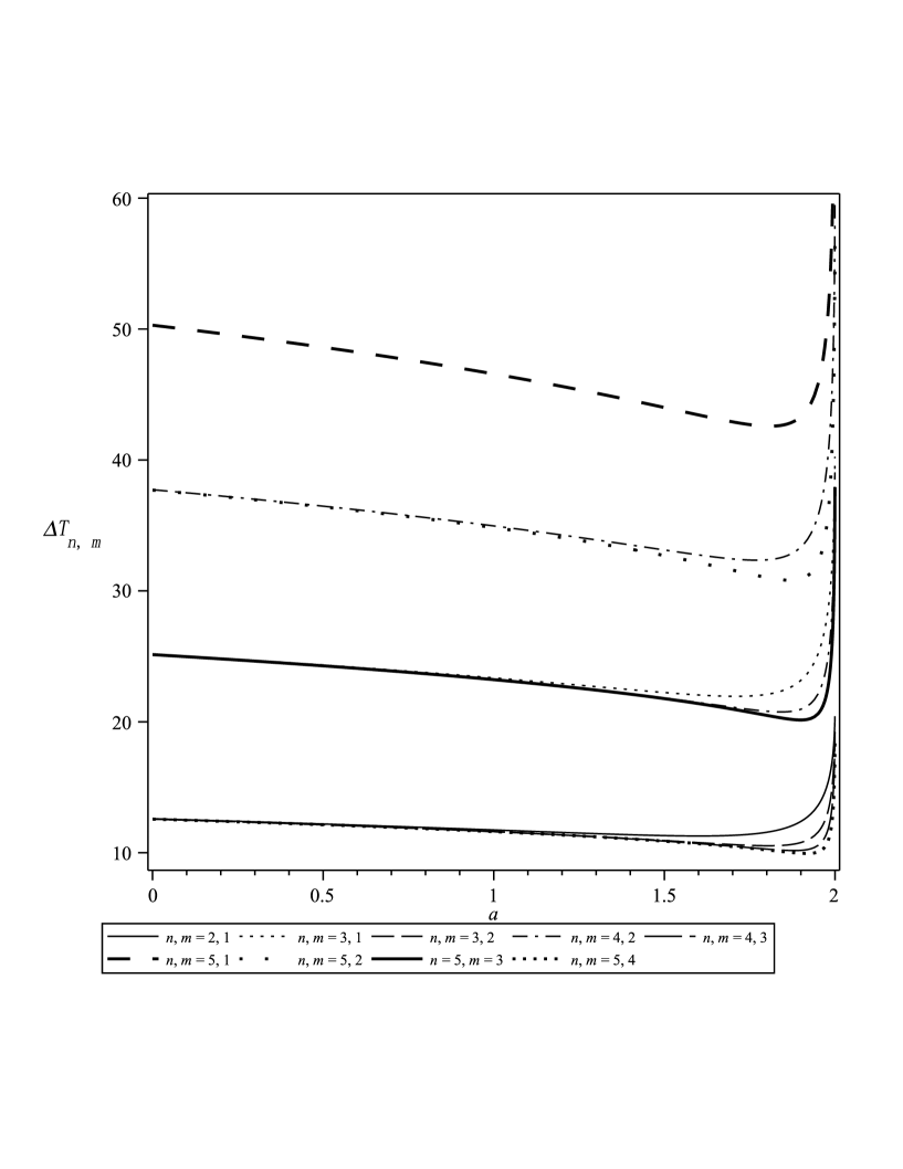
Figure 1: The curves of time delay as a function of Gauss-Bonnet coupling $a=\frac{\alpha}{M}$ limited by $a\in[0,2)$.

References

- [1] P. Schneider, J. Ehlers, E. E. Falco, Gravitational Lenses, Springer-Verlag, Berlin, 1992
- [2] S. Mollerach, E. Roulet, Gravitational Lensing and Microlensing, World Scientific Publishing Co. Pte. Ltd. 2002
- [3] R. D. Blandford, R. Narayan, Annu. Rev. Astron. Astrophys. 30(1992)311
- [4] S. Refsdal, J. Surdej, Rep. Prog. Phys. 56(1994)117
- [5] C. Darwin, Proc. Roy. Soc. Lond. 249(1959)180
- [6] S. U. Viergutz, Astron. Astrophys. 272(1993)355
- [7] H. Falcke, F. Melia, E. Agol, Astrophys. J. Lett. 528(2000)L13
- [8] K. S. Virbhadra, G. F. R. Ellis, Phys. Rev. D62(2000)084003
- [9] V. Bozza, S. Capozziello, G. Iovane, G. Scarpetta, Gen. Rel. Grav. 33(2001)1535
- [10] V. Bozza, Phys. Rev. D66(2002)103001
- [11] S. Frittelli, T. P. Kling, T. Newman, Phys. Rev. D61(2000)064021
- [12] K. S. Virbhadra, G. F. R. Ellis, Phys. Rev. D65(2002)103004
- [13] E. F. Eiroa, G. E. Romero, D. F. Torres, Phys. Rev. D66(2002)024010
- [14] A. Bhadra, Phys. Rev. D67(2003)103009
- [15] V. Bozza, Phys. Rev. D67(2003)103006
- [16] V. Bozza, F. Deluca, G. Scarpetta, M. Sereno, Phys. Rev. D72(2005)083003
- [17] R. Whisker, Phys. Rev. D71(2005)064004
- [18] E. F. Eiroa, Phys. Rev. D71(2005)083010
- [19] E. F. Eiroa, Phys. Rev. D73(2006)043002
- [20] K. Sarkar, A. Bhadra, Class. Quantum Grav. 23(2006)6101
- [21] V. Perlick, Phys. Rev. D69(2004)064017
- [22] H. Cheng, J. Man, Class. Quantum Grav. 28(2011)015001
- [23] S. Chen, J. Jing, Phys. Rev. D80(2009)024036
- [24] J. Sadeghi, H. Vaez, JCAP1406(2014)028
- [25] E. Abdalla, R. A. Konoplya, Phys. Rev. D72(2005)084006
- [26] R. J. Gleiser, G. Dotti, Phys. Rev. D72(2005)124002
- [27] C. Sahabandu, P. Suranyi, C. Vaz, L. C. R. Wijewardhana, Phys. Rev. D73(2006)044009
- [28] A. E. Dominguez, E. Gallo, Phys. Rev. D73(2006)064018
- [29] H. Maeda, N. Dadhich, Phys. Rev. D74(2006)021501
- [30] H. Cheng, Y. Liu, Chin. Phys. Lett. 25(2008)1160
- [31] D. G. Boulware, S. Deser, Phys. Rev. Lett. 55(1985)2656
- [32] S. Weinberg, Gravitation and Cosmology: Principles and Applications of the General Theory of Relativity, Wiley, New York, 1972