Parallel Distributed Block Coordinate Descent Methods based on Pairwise Comparison Oracle

Abstract

This paper provides a block coordinate descent algorithm to solve unconstrained optimization problems. In our algorithm, computation of function values or gradients is not required. Instead, pairwise comparison of function values is used. Our algorithm consists of two steps; one is the direction estimate step and the other is the search step. Both steps require only pairwise comparison of function values, which tells us only the order of function values over two points. In the direction estimate step, a Newton type search direction is estimated. A computation method like block coordinate descent methods is used with the pairwise comparison. In the search step, a numerical solution is updated along the estimated direction. The computation in the direction estimate step can be easily parallelized, and thus, the algorithm works efficiently to find the minimizer of the objective function. Also, we show an upper bound of the convergence rate. In numerical experiments, we show that our method efficiently finds the optimal solution compared to some existing methods based on the pairwise comparison.

1 Introduction

Recently, demand for large-scale complex optimization is increasing in computational science, engineering and many of other fields. In that kind of problems, there are many difficulties caused by noise in function evaluation, many tuning parameters and high computation cost. In such cases, derivatives of the objective function are unavailable or computationally infeasible. These problems can be treated by the derivative-free optimization (DFO) methods.

DFO is the tool for optimization without derivative information of the objective function and constraints, and it has been widely studied for decades [3, 17]. DFO algorithms include gradient descent methods with a finite difference gradient estimation [6, 5], some direct search methods using only function values [1, 13], and trust-region methods [4].

There is, however, a more restricted setting in which not only derivatives but also values of the objective function are unavailable or computationally infeasible. In such a situation, the so-called pairwise comparison oracle, that tells us an order of function values on two evaluation points, is used instead of derivatives and function evaluation [13, 8]. For example, the pairwise comparison is used in learning to rank to collect training samples to estimate the preference function of the ranking problems [12]. In decision making, finding the most preferred feasible solution from among the set of many alternatives is an important application of ranking methods using the pairwise comparison. Also, other type of information such as stochastic gradient-sign oracle has been studied [15].

Now, let us introduce two DFO methods, i.e., the Nelder-Mead method [13] and stochastic coordinate descent algorithm [8]. They are closely related to our work. In both methods, the pairwise comparison of function values is used as a building block in optimization algorithms.

Nelder and Mead’s downhill simplex method [13] was proposed in early study of algorithms based on the pairwise comparison of function values. In each iteration of the algorithm, a simplex that approximates the objective function is constructed according to ranking of function values on sampled points. Then, the simplex receives four operations, namely, reflection, expansion, contraction and reduction in order to get close to the optimal solution. Unfortunately, the convergence of the Nelder-Mead algorithm is theoretically guaranteed only in low-dimension problems [10]. In high dimensional problems, the Nelder-Mead algorithm works poorly as shown in [7].

The stochastic coordinate descent algorithm using only the noisy pairwise comparison was proposed in [8]. Lower and upper bounds of the convergence rate were also presented in terms of the number of pairwise comparison of function values, i.e., query complexity. The algorithm iteratively solves one dimensional optimization problems like the coordinate descent method. However, practical performance of the optimization algorithm was not studied in that work.

In this paper, we focus on optimization algorithms using the pairwise comparison oracle. In our algorithm, the convergence to the optimal solution is guaranteed, when the number of pairwise comparison tends to infinity. Our algorithm is regarded as a block coordinate descent method consisting of two steps: the direction estimate step and search step. In the direction estimate step, the search direction is determined. In the search step, the current solution is updated along the search direction with an appropriate step length. In our algorithm, the direction estimate step is easily parallelized. Therefore, it is expected that our algorithm effectively works even in large-scale optimization problems.

Let us summarize the contributions presented in this paper.

1. We propose a block coordinate descent algorithm based on the pairwise comparison oracle, and point out that the algorithm is easily parallelized.

2. We derive an upper bound of the convergence rate in terms of the number of pairwise comparison of function values, i.e., query complexity.

3. We show a practical efficiency of our algorithm through numerical experiments.

The rest of the paper is organized as follows. In Section 2, we explain the problem setup and give some definitions. Section 3 is devoted to the main results. The convergence properties and query complexity of our algorithm are shown in the section. In Section 4, numerical examples are reported. Finally in Section 5, we conclude the paper with the discussion on future works. All proofs of theoretical results are found in appendix.

2 Preliminaries

In this section, we introduce the problem setup and prepare some definitions and notations used throughout the paper. A function $f:\mathbb{R}^{n}\rightarrow\mathbb{R}$ is said to be $\sigma$-strongly convex on $\mathbb{R}^{n}$ for a positive constant $\sigma$, if for all ${\bm{x}},{\bm{y}}\in\mathbb{R}^{n}$, the inequality

$$f({\bm{y}})\geq f({\bm{x}})+\nabla f({\bm{x}})^{T}({\bm{y}}-{\bm{x}})+\frac{\sigma}{2}\|{\bm{x}}-{\bm{y}}\|^{2}$$

holds, where $\nabla f({\bm{x}})$ and $\|\cdot\|$ denote the gradient of $f$ at ${\bm{x}}$ and the euclidean norm, respectively. The function $f$ is $L$-strongly smooth for a positive constant $L$, if $\|\nabla f({\bm{x}})-\nabla f({\bm{y}})\|\leq{}L\|{\bm{x}}-{\bm{y}}\|$ holds for all ${\bm{x}},{\bm{y}}\in\mathbb{R}^{n}$. The gradient $\nabla{f({\bm{x}})}$ of the $L$-strongly smooth function $f$ is referred to as $L$-Lipschitz gradient. The class of $\sigma$-strongly convex and $L$-strongly smooth functions on $\mathbb{R}^{n}$ is denoted as $\mathcal{F}_{\sigma,L}({\mathbb{R}}^{n})$. In the convergence analysis, mainly we focus on the optimization of objective functions in $\mathcal{F}_{\sigma,L}({\mathbb{R}}^{n})$.

We consider the following pairwise comparison oracle defined in [8].

Definition 1 (Pairwise comparison oracle).

The stochastic pairwise comparison (PC) oracle is a binary valued random variable $O_{f}:\mathbb{R}^{n}\times\mathbb{R}^{n}\rightarrow\{\ -1,+1\}$ defined as

$$\mathrm{Pr}[O_{f}({\bm{x}},{\bm{y}})={\rm sign}\{f({\bm{y}})-f({\bm{x}})\}]\geq\frac{1}{2}+\min\{\delta_{0},\mu|f({\bm{y}})-f({\bm{x}})|^{\kappa-1}\},$$ (1)

where $0<\delta_{0}\leq 1/2$, $\mu>0$ and $\kappa\geq 1$. For $\kappa=1$, without loss of generality $\mu\leq\delta_{0}\leq 1/2$ is assumed. When the equality

$$\mathrm{Pr}[O_{f}({\bm{x}},{\bm{y}})={\rm sign}\{f({\bm{y}})-f({\bm{x}})\}]=1$$ (2)

is satisfied for all ${\bm{x}}$ and ${\bm{y}}$, we call $O_{f}$ the deterministic PC oracle.

For $\kappa=1$, the probability in (1) is not affected by the difference $|f({\bm{y}})-f({\bm{x}})|$, meaning that the probability for the output of the PC oracle is not changed under any monotone transformation of $f$.

In [8], Jamieson et al. derived lower and upper bounds of convergence rate of an optimization algorithm using the stochastic PC oracle. The algorithm is referred to as the original PC algorithm in the present paper.

Under above preparations, our purpose is to find the minimizer ${\bm{x}}^{*}$ of the objective function $f({\bm{x}})$ in $\mathcal{F}_{\sigma,L}({\mathbb{R}}^{n})$ by using PC oracle. In the following section, we provide a DFO algorithm in order to solve the optimization problem and consider the convergence properties including query complexity.

3 Main Results

3.1 Algorithm

Algorithm 1 Block coordinate descent using PC oracle (BlockCD[$n$, $m$])

  Input: initial point ${\bm{x}}_{0}\in\mathbb{R}^{n}$, and accuracy in line search $\eta>0$.

  Initialize: set $t=0$.

  repeat

     Choose $m$ coordinates ${i_{1}},\ldots,{i_{m}}$ out of $n$ coordinates according to the uniform distribution.

     (Direction estimate step)

     [Step D-1] Solve the one-dimension optimization problems

$$\min_{\alpha\in\mathbb{R}}f({\bm{x}}_{t}+\alpha{\bm{e}}_{i_{k}}),\quad k=1,\ldots,m,$$ (3)

within the accuracy $\eta/2$ using the PC-based line search algorithm shown in Algorithm 2, where ${\bm{e}}_{i}$ denotes the $i$-th unit basis vector. Then, obtain the numerical solutions $\alpha_{t,i_{k}},k=1,\ldots,m$.

     [Step D-2] Set ${\bm{d}}_{t}=\sum_{k=1}^{m}\alpha_{t,i_{k}}{\bm{e}}_{i_{k}}$. If ${\bm{d}}_{t}$ is the zero vector, add $\eta/2$ to $d_{i_{1}}$.

     (Search step)

     [Step S-1] Apply Algorithm 2 to obtain a numerical solution $\beta_{t}$ of

$$\min_{\beta}f({\bm{x}}_{t}+\beta{\bm{d}}_{t}/\|{\bm{d}}_{t}\|)$$

within the accuracy $\eta$.

     [Update] ${\bm{x}}_{t+1}={\bm{x}}_{t}+\beta_{t}{\bm{d}}_{t}/\|{\bm{d}}_{t}\|;\ t\leftarrow{t+1}$.

  until A stopping criterion is satisfied.

  Output: ${\bm{x}}_{t}$

In Algorithm 1, we propose a DFO algorithm based on the PC oracle. In our algorithm, $m$ coordinates out of $n$ elements are updated in each iteration to efficiently cope with high dimensional problems. Algorithm 1 is referred to as $\mathrm{BlockCD}[n,m]$. The original PC algorithm is recovered by setting $m=1$. The PC oracle is used in the line search algorithm to solve one-dimensional optimization problems; the detailed line search algorithm is shown in Algorithm 2.

For $m=n$, the search direction ${\bm{d}}_{t}$ in Algorithm 1 approximates that of a modified Newton method [11, Chap. 10], as shown below. In Step D-1 of the algorithm, one-dimensional optimization problems (3) are solved. Let $\alpha_{t,i}^{*}$ be the optimal solution of (3) with $i_{k}=i$. Then, $\alpha_{t,i}^{*}$ will be close to the numerical solution $\alpha_{t,i}$. The Taylor expansion of the objective function leads to

$$f({\bm{x}}_{t}+\alpha{\bm{e}}_{i})=f({\bm{x}}_{t})+\alpha{\bm{e}}_{i}^{T}\nabla{f}({\bm{x}}_{t})+\frac{\alpha^{2}}{2}{\bm{e}}_{i}^{T}\nabla^{2}{f}({\bm{x}}_{t}){\bm{e}}_{i}+o(\alpha^{2}),$$

where $\nabla^{2}{f}({\bm{x}}_{t})$ is the Hessian matrix of $f$ at ${\bm{x}}_{t}$. When the point ${\bm{x}}_{t}$ is close to the optimal solution of $f({\bm{x}})$, the optimal parameter $\alpha_{i,t}^{*}$ will be close to zero, implying that the higher order term $o(\alpha^{2})$ in the above is negligible. Hence, $\alpha_{t,i}$ is approximated by the optimal solution of the quadratic approximation, i.e., $-(\nabla{f}({\bm{x}}_{t}))_{i}/(\nabla^{2}f({\bm{x}}_{t}))_{ii}$. As a result, the search direction in $\mathrm{BlockCD}[n,n]$ is approximated by $-({\mathrm{diag}}(\nabla^{2}{f}({\bm{x}}_{t})))^{-1}\nabla{f}({\bm{x}}_{t})$, where $\mathrm{diag}(A)$ denotes the diagonal matrix, the diagonal elements of which are those of the square matrix $A$. In the modified Newton method, the Hessian matrix in the Newton method is replaced with a positive definite matrix to reduce the computation cost. Using only the diagonal part of the Hessian matrix is a popular choice in the modified Newton method.

Algorithm 2 line search algorithm using PC oracle [8]

  Input: current solution ${\bm{x}}_{t}\in\mathbb{R}^{n}$, search direction ${\bm{d}}\in\mathbb{R}^{n}$ and accuracy in line search $\eta>0$.

  Initialize: set $\alpha_{0}=0$, $\alpha^{+}_{0}=\alpha_{0}+1$, $\alpha^{-}_{0}=\alpha_{0}-1$, $k=0$.

  [Step1]

  if $O_{f}({\bm{x}}_{t},{\bm{x}}_{t}+\alpha^{+}_{0}{\bm{d}})>0$ and $O_{f}({\bm{x}}_{t},{\bm{x}}_{t}+\alpha^{-}_{0}{\bm{d}})<0$ then

     $\alpha^{+}_{0}\leftarrow 0$

  else if $O_{f}({\bm{x}}_{t},{\bm{x}}_{t}+\alpha^{+}_{0}{\bm{d}})<0$ and $O_{f}({\bm{x}}_{t},{\bm{x}}_{t}+\alpha^{-}_{0}{\bm{d}})>0$ then

     $\alpha^{-}_{0}\leftarrow 0$

  end if

  [Step2] (double-sign corresponds)

  while $O_{f}({\bm{x}}_{t},{\bm{x}}_{t}+\alpha^{\pm}_{k}{\bm{d}})<0$ do

     $\alpha^{\pm}_{k+1}\leftarrow 2\alpha^{\pm}_{k}$, $k\leftarrow k+1$

  end while

  [Step3]

  while $|\alpha^{+}_{k}-\alpha^{-}_{k}|>\eta/2$ do

     if $O_{f}({\bm{x}}_{t}+\alpha_{k}{\bm{d}},{\bm{x}}_{t}+\frac{1}{2}(\alpha_{k}+\alpha^{+}_{k}){\bm{d}})<0$ then

        $\alpha_{k+1}\leftarrow\frac{1}{2}(\alpha_{k}+\alpha^{+}_{k})$, $\alpha^{+}_{k+1}\leftarrow\alpha^{+}_{k}$, $\alpha^{-}_{k+1}\leftarrow\alpha_{k}$

     else if $O_{f}({\bm{x}}_{t}+\alpha_{k}{\bm{d}},{\bm{x}}_{t}+\frac{1}{2}(\alpha_{k}+\alpha^{-}_{k}){\bm{d}})<0$ then

        $\alpha_{k+1}\leftarrow\frac{1}{2}(\alpha_{k}+\alpha^{-}_{k})$, $\alpha^{-}_{k+1}\leftarrow\alpha^{-}_{k}$, $\alpha^{+}_{k+1}\leftarrow\alpha_{k}$

     else

        (double-sign corresponds)

        $\alpha_{k+1}\leftarrow\alpha_{k}$, $\alpha^{\pm}_{k+1}\leftarrow\frac{1}{2}(\alpha_{k}+\alpha^{\pm}_{k})$

     end if

  end while

  Output: $\alpha_{t}$

Figure 1 demonstrates an example of the optimization process of both the original PC algorithm and our algorithm. The original PC algorithm updates the numerical solution along a randomly chosen coordinate in each iteration. Hence, many iterations are required to get close to the optimal solution. On the other hand, in our algorithm, a solution can move along a oblique direction. Therefore, our algorithm can get close to the optimal solution with less iterations than the original PC algorithm.

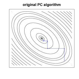
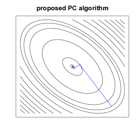
Figure 1: A behavior of the algorithms on the contour of the quadratic objective function $x_{1}^{2}+x_{2}^{2}+x_{1}x_{2}$ with same initialization. Left panel: Jamieson et al.’s original PC algorithm. Right panel: proposed algorithm.

3.2 Convergence Properties of our Algorithm under Deterministic Oracle

We now provide an upper bound of the convergence rate of our algorithm using the deterministic PC oracle (2). Let us denote the minimizer of $f$ as ${\bm{x}}^{*}$.

Theorem 1.

Suppose $f\in\mathcal{F}_{\sigma,L}(\mathbb{R}^{n})$, and define $\gamma$ and $\varepsilon$ be

$$\gamma=\frac{\sigma/L}{53}\left(\frac{1-\sqrt{1-\sigma/L}}{1+\sqrt{1-\sigma/L}}\right)^{2},\quad\varepsilon=\frac{8nL^{2}}{\sigma}\bigg{(}1+\frac{n}{m\gamma}\bigg{)}\eta^{2}.$$

Let us define $T_{0}$ be

$$T_{0}=\bigg{\lceil}\frac{n}{m\gamma}\log\frac{(f({\bm{x}}_{0})-f({\bm{x}}^{*}))(1+\frac{n}{m\gamma})}{\varepsilon}\bigg{\rceil}.$$ (4)

For $T\geq{T_{0}}$, we have $\mathbb{E}[f({\bm{x}}_{T})-f({\bm{x}}^{*})]\leq{}\varepsilon$, where the expectation is taken with respect to the random choice of coordinates $i_{1},\ldots,i_{k}$ to be updated in $\mathrm{BlockCD}[n,m]$.

The proof of Theorem 1 is given in A. Note that any monotone transformation of the objective function does not affect the output of the deterministic PC oracle. Hence, the theorem above holds even for the function $f({\bm{x}})$ such that the composite function with a monotone function is included in $\mathcal{F}_{\sigma,L}({\mathbb{R}}^{n})$.

3.3 Query Complexity

Let $\hat{{\bm{x}}}_{Q}$ be the output of BlockCD$[n,m]$ after $Q$ pairwise comparison queries. To solve the one dimension optimization problem within the accuracy $\eta/2$, the sufficient number of the call of PC-oracle is

$$K_{0}=2\log_{2}\frac{2^{10}L(f({\bm{x}}_{0})-f({\bm{x}}^{*}))}{\sigma^{2}\eta^{2}},$$

as shown in [8]. Hence, if the inequality $Q\geq{}T_{0}K_{0}(m+1)$ holds, Theorem 1 assures that the numerical solution $\hat{{\bm{x}}}_{Q}$ based on $Q$ queries satisfies

$$\mathbb{E}[f(\hat{{\bm{x}}}_{Q})-f({\bm{x}}^{*})]\leq\varepsilon.$$

When $n/\varepsilon$ is sufficiently large, we have

$$\phantom{=}T_{0}K_{0}(m+1)$$

$$=(m+1)\bigg{\lceil}\frac{n}{m\gamma}\log\frac{(f({\bm{x}}_{0})-f({\bm{x}}^{*}))(1+\frac{n}{m\gamma})}{\varepsilon}\bigg{\rceil}\cdot\bigg{\lceil}2\log_{2}\frac{2^{10}L(f({\bm{x}}_{0})-f({\bm{x}}^{*}))}{\sigma^{2}\eta^{2}}\bigg{\rceil}$$

$$=(m+1)\bigg{\lceil}\frac{n}{m\gamma}\log\frac{\Delta_{0}(1+\frac{n}{m\gamma})}{\varepsilon}\bigg{\rceil}\cdot\bigg{\lceil}2\log_{2}\frac{2^{13}(L/\sigma)^{3}\Delta_{0}n(1+\frac{n}{m\gamma})}{\varepsilon}\bigg{\rceil}$$

$$\leq c_{0}n\left(\log\frac{n}{\varepsilon}\right)^{2}\leq c_{0}n(\log{n})^{2}\left(\log\frac{1}{\varepsilon}\right)^{2},$$

where $c_{0}$ is a constant depending on $L/\sigma$ and $\Delta_{0}=f({\bm{x}}_{0})-f({\bm{x}}^{*})$. The last inequality holds if $\log{n}$ and $\log(1/\varepsilon)$ are both greater than $2$. Eventually we have

$$\mathbb{E}[f(\hat{{\bm{x}}}_{Q})-f({\bm{x}}^{*})]\leq{}\exp\left\{-\frac{c}{\log{n}}\sqrt{\frac{Q}{n}}\right\},$$ (5)

where $c=1/\sqrt{c_{0}}$. The above bound is of the same order of the convergence rate for the original PC algorithm up to polylog factors. On the other hand, a lower bound presented in [8] is of order $e^{-cQ/n}$ with a positive constant $c$ up to polylog factors, when the PC oracle with $\kappa=1$ is used.

In Theorem 1, it is assumed that the objective function is strongly convex and gradient Lipschitz. In a realistic situation, we usually do not have the knowledge of the class parameters $\sigma$ and $L$ of the unknown objective function. Moreover, strong convexity and gradient Lipschitzness on the whole space ${\mathbb{R}}^{n}$ is too strong. In the following corollary, we relax the assumption in Theorem 1 and prove the convergence property of our algorithm without strong convexity and strong smoothness.

Corollary 1.

Let $f:{\mathbb{R}}^{n}\to{\mathbb{R}}$ be a twice continuously differentiable convex function with non-degenerate Hessian on ${\mathbb{R}}^{n}$ and ${\bm{x}}^{*}$ be a minimizer of $f$. Then, there is a constant $c$ such that the output $\hat{x}_{Q}$ of BlockCD[n,m] satisfies (5).

The proof of Corollary 1 is given in B.

3.4 Generalization to Stochastic Pairwise Comparison Oracle

Algorithm 3 Repeated querying subroutine ([8, 9])

  Input: ${\bm{x}},{\bm{y}}\in\mathbb{R}^{n}$, $p={\rm Pr}[O_{f}({\bm{x}},{\bm{y}})={\rm sign}\{f({\bm{y}})-f({\bm{x}})\}]$, $\delta>0$

  Initialize: set $n_{0}=1$ and toss the coin with probability $p$ of heads once.

  for $k=0,1,...$ do

      $p_{k}=\mbox{frequency of heads in all tosses so far}$

     $I_{k}=\left[p_{k}-\sqrt{\frac{(k+1)\log(2/\delta)}{2^{k}}},p_{k}+\sqrt{\frac{(k+1)\log(2/\delta)}{2^{k}}}\right]$

     if $\frac{1}{2}\not\in I_{k}$ then

        break

     else

        toss the coin $n_{k}$ more times, and set $n_{k+1}=2n_{k}$.

     end if

  end for

  if $p_{k}+\sqrt{\frac{(k+1)\log(2/\delta)}{2^{k}}}\leq\frac{1}{2}$ then

     return $-1$

  else

     return $+1$

  end if

In stochastic PC oracle, one needs to ensure that the correct information is obtained in high probability. In Algorithm 3, the query $O_{f}({\bm{x}},{\bm{y}})$ is repeated under the stochastic PC oracle. The reliability of line search algorithm based on stochastic PC oracle (1) was investigated by [8, 9].

Lemma 1 ([8, 9]).

For any ${\bm{x}},{\bm{y}}\in\mathbb{R}^{n}$ with $p={\rm Pr}[O_{f}({\bm{x}},{\bm{y}})={\rm sign}\{f({\bm{y}})-f({\bm{x}})\}]$, the repeated querying subroutine in Algorithm 3 correctly identifies the sign of $\mathbb{E}[O_{f}({\bm{x}},{\bm{y}})]$ with probability $1-\delta$, and requests no more than

$$\frac{\log{2/\delta}}{4|1/2-p|^{2}}\log_{2}\left(\frac{\log{2/\delta}}{4|1/2-p|^{2}}\right)$$ (6)

queries.

It should be noted here that, in this paper, ${\rm sign}\{E[O_{f}(x,y)]\}={\rm sign}\{f(y)-f(x)\}$ always holds because $p>1/2$ from (1). In [8], a modified line search algorithm using a ternary search instead of bisection search was proposed to lower bound $|1/2-p|$ in Lemma 1 for arbitrary ${\bm{x}},{\bm{y}}\in\mathbb{R}^{n}$. Then, one can find that the total number of queries required by a repeated querying subroutine algorithm is at most $\tilde{O}\left(\frac{\log{1/\delta}}{\eta^{4(\kappa-1)}}\right)$, where $\eta$ is an accuracy of line search. The query complexity of the stochastic PC oracle is obtained from that of the deterministic PC oracle. Suppose that one has $Q_{0}$ responses from the deterministic PC oracle. To obtain the same responses from the stochastic PC oracle with probability more than $1-\delta$, one needs more than $\tilde{O}(Q_{0}\eta^{-4(\kappa-1)}\log(\frac{Q_{0}}{\delta}))$ queries. From the above discussion, we have the following upper bounds for stochastic setting:

$$\mathbb{E}[f(\hat{{\bm{x}}}_{Q})-f({\bm{x}}^{*})]\leq\begin{cases}\displaystyle\exp\left\{-\frac{c_{1}}{\log{n}}\sqrt{\frac{Q}{n}}\right\},&\kappa=1,\vspace*{2mm}\\ \displaystyle c_{2}\displaystyle\frac{n^{2}}{m}\left(\frac{n}{Q}\right)^{1/(2\kappa-2)},&\kappa>1,\end{cases}$$ (7)

where $c_{1}$ and $c_{2}$ are constant depending on $L/\sigma$ and $f({\bm{x}}_{0})-f({\bm{x}}^{*})$ as well as $1/\delta$ poly-logarithmically. If $m$ and $n$ are of the same order in the case of $\kappa>1$, the bound (7) coincides with that shown in Theorem 2 of [8].

4 Numerical Experiments

In this section, we present numerical experiments in which the proposed method in Algorithm 1 was mainly compared with the Nelder-Mead algorithm [13] and the original PC algorithm [8], i.e., BlockCD$[n,1]$ of Algorithm 1. Here, the PC oracle was used in all the optimization algorithms. In BlockCD$[n,m]$ with $m\geq 2$, one can execute the line search algorithm to each axis separately. Hence, the parallel computation is directly available to find the components of the search direction ${\bm{d}}_{t}$. Also, we investigated the computation efficiency of the parallel implementation of our method. The numerical experiments were conducted on AMD Opteron Processor 6176 (2.3GHz) with 48 cores, running Cent OS Linux release 6.4. We used the R language [14] with snow library for parallel statistical computing.

4.1 Two Dimensional Problems

It is well-known that the Nelder-Mead method efficiently works in low dimensional problems. Indeed, in our preliminary experiments for two dimensional optimization problems, the Nelder-Mead method showed a good convergence property compared to the other methods such as BlockCD$[2,m]$ with $m=1,2$. Numerical results are presented in Figure 2. We tested optimization methods on the quadratic function $f(x)=x^{T}Ax$, and two-dimension Rosenbrock function, $f(x)=(1-x_{1})^{2}+100(x_{2}-x_{1}^{2})^{2}$, where the matrix $A$ was a randomly generated 2 by 2 positive definite matrix. In two dimension problems, we do not use the parallel implementation of our method, since clearly the parallel computation is not efficient that much. The efficiency of parallel computation is canceled by the communication overhead. In our method, the accuracy of the line search is fixed to a small positive number $\eta$. Hence, the optimization process stops on the way to the optimal solution, as shown in the left panel of Fig. 2. On the other hand, the Nelder-Mead method tends to converge to the optimal solution in high accuracy. In terms of the convergence speed for the optimization of two-dimensional quadratic function, there is no difference between the Nelder-Mead method and BlockCD method, until the latter stops due to the limitation of the numerical accuracy. Even in non-convex Rosenbrock function, the Nelder-Mead method works well compared to the PC-based BlockCD algorithm.

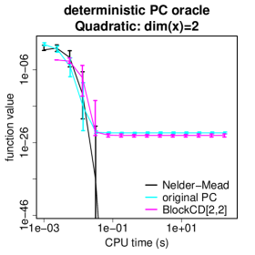
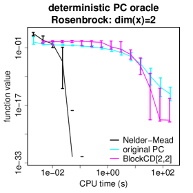
Figure 2: Left panel: 2-dimension quadratic function. Right panel: 2-dimension Rosenbrock function. The Nelder-Mead method, BlockCD$[2,1]$, and BlockCD$[2,2]$ are compared. For each algorithm, the median of the function value is depicted to the CPU time (s). The vertical bar shows the percentile $30\%$ to $70\%$.

4.2 Numerical Experiments of Parallel Computation

In high dimensional problems, however, the performance of the Nelder-Mead method is easily degraded as reported by several authors; see [7] and references therein. In the below, we focus on solving moderate-scale optimization problems.

In experiments using the PC oracle, BlockCD$[n,m]$ with $m\geq 2$ and its parallel implementations were compared with the Nelder-Mead method and the original PC algorithm, i.e., BlockCD$[n,1]$. In each iteration of BlockCD$[n,m]$ with $m\geq 2$, $m+1$ runs of the line search were required. In the parallel implementation, tasks of line search except the search step in Algorithm 1 were almost equally assigned to each core in processors. In the below, the parallel implementation of BlockCD$[n,m]$ is referred to as parallel-BlockCD$[n,m]$. Suppose that $c$ cores are used in parallel-BlockCD$[n,m]$. Then, ideally, the parallel computation will be approximately $(m+1)/(m/c+1)\approx{c}$ times more efficient than the serial processing, when $n$ and $m$ are much greater than $c$. Practically, however, the communication overhead among processors may cancel the effect of the parallel computation, especially in small-scale problems.

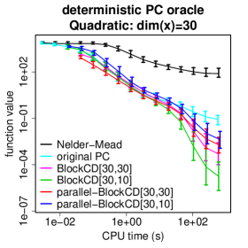
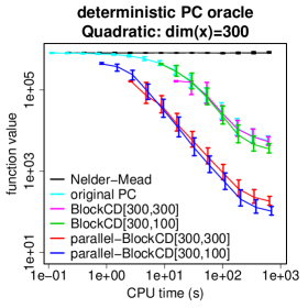
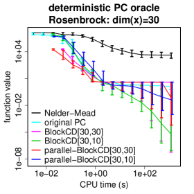
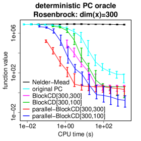
Figure 3: Deterministic PC oracle is used in PC-based BlockCD algorithm. Top panels: results in optimization of quadratic function. Bottom panels: results in optimization of Rosenbrock function. The original PC algorithm, BlockCD$[n,m]$ with $m=n$ and $m=n/3$, and parallel-BlockCD$[n,m]$ with $m=n$ and $m=n/3$, are compared for $n=30$ and $n=300$. The median of the function value is shown to the CPU time (s). The vertical bar shows the percentile $30\%$ to $70\%$.

We tested optimization methods on two $n$-dimensional optimization problems, i.e., the quadratic function $f(x)=x^{T}Ax$, and Rosenbrock function, $f(x)=\sum_{i=1}^{n-1}[(1-x_{i})^{2}+100(x_{i+1}-x_{i}^{2})^{2}]$, where the matrix $A$ was a randomly generated $n$ by $n$ positive definite matrix. The quadratic function satisfies the assumptions in Theorem 1, while the Rosenbrock function is not convex. We examine whether the proposed method is efficient even when the theoretical assumptions are not necessarily assured. In each objective function, the dimension was set to $n=30$ or $300$. In all problems, the optimal value is zero. For each algorithm, the optimization was repeated 10 times using randomly chosen initial points. According to [7], we examined some tuning parameters for the Nelder-Mead algorithm, and we found that the initial simplex does not significantly affect the numerical results in the present experiments. Hence, the standard parameter setting of the Nelder-Mead method used in [7] was used throughout the present experiments.

The numerical results using the deterministic PC oracle are presented in Figure 3. For each algorithm, the median of function values in optimization process is depicted as the solid line with 30 and 70 percentiles for each CPU time. The results indicate that the Nelder-Mead method does not efficiently work even for 30-dimensional quadratic function. The original PC algorithm and serially executed BlockCD$[n,m]$ were comparable. This result is consistent with (5). When the deterministic PC oracle is used, the upper bound of the query complexity is independent of $m$. As for the efficiency of the parallel computation, the parallel-BlockCD$[n,m]$ outperformed the competitors in 300 dimensional problems. In our experiments, the parallel implementation was about 15 times more efficient than the serial implementation in CPU time. For large-scale problems, the communication overhead is canceled by the efficiency of the parallel computation. In our approach, the parallel computation is easily conducted without losing the convergence property proved in Theorem 1.

Also, we conducted optimization using the stochastic PC oracle. The results are shown in Fig. 4. The parameter in the stochastic PC oracle was set to $\kappa=2,\delta_{0}=0.3$ and $\mu=0.01$. Thus, the difference of two function values affects the probability that the oracle returns the correct sign. According to Lemma 1, the query was repeated at each point so that the probability of receiving the correct sign was greater than $1-\delta$ with $\delta=0.01$. As shown in the results of $\mathrm{BlockCD}[300,100]$ and $\mathrm{BlockCD}[300,300]$, the serial implementation of $\mathrm{BlockCD}[n,m]$ for a large $m$ was extremely inefficient. Indeed, the right panels of Fig. 4 indicate that an iteration of $\mathrm{BlockCD}[300,300]$ takes a long time. Also, the convergence rate of the original PC algorithm was slow, though the computational cost of each iteration was not high. When the stochastic PC oracle was used, the parallel implementation of BlockCD$[n,m]$ achieved fast convergence rate compared with the other algorithms in CPU time.

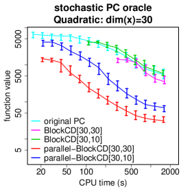
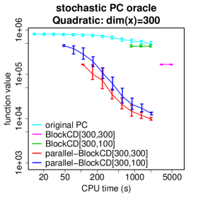
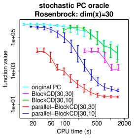
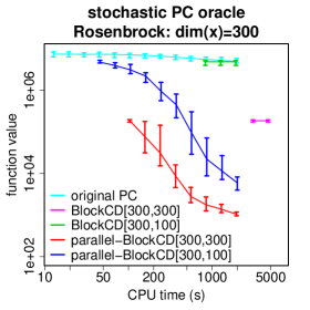
Figure 4: Stochastic PC oracle is used in PC-based BlockCD algorithm. Top panels: results in optimization of quadratic function. Bottom panels: results in optimization of Rosenbrock function. The original PC algorithm, BlockCD$[n,m]$ with $m=n$ and $m=n/3$, and parallel-BlockCD$[n,m]$ with $m=n$ and $m=n/3$, are compared for $n=30$ and $n=300$. The median of the function value is shown to the CPU time (s). The vertical bar shows the percentile $30\%$ to $70\%$.

5 Conclusion

In this paper, we proposed a block coordinate descent algorithm for unconstrained optimization problems using the pairwise comparison of function values. Our algorithm consists of two steps: the direction estimate step and search step. The direction estimate step can easily be parallelized. Hence, our algorithm is effectively applicable to large-scale optimization problems. Theoretically, we obtained an upper bound of the convergence rate and query complexity, when the deterministic and stochastic pairwise comparison oracles were used. Practically, our algorithm is simple and easy to implement. In addition, numerical experiments showed that the parallel implementation of our algorithm outperformed the other methods. An extension of our algorithm to constrained optimization problems is an important future work. Other interesting research directions include pursuing the relation between pairwise comparison oracle and other kind of oracles such as gradient-sign oracle [16].

Appendix A Proof of Theorem 1

Proof.

The optimal solution of $f$ is denoted as ${\bm{x}}^{*}$. Let us define $\varepsilon^{\prime}$ be $\varepsilon/(1+\frac{n}{m\gamma})$. If $f({\bm{x}}_{t})-f({\bm{x}}^{*})<\varepsilon^{\prime}$ holds in the algorithm, we obtain $f({\bm{x}}_{t+1})-f({\bm{x}}^{*})<\varepsilon^{\prime}$, since the function value is non-increasing in each iteration of the algorithm.

Next, we assume $\varepsilon^{\prime}\leq{}f({\bm{x}}_{t})-f({\bm{x}}^{*})$. The assumption leads to

$$2\sigma\varepsilon^{\prime}\leq 2\sigma(f({\bm{x}}_{t})-f({\bm{x}}^{*}))\leq\|\nabla{f}({\bm{x}}_{t})\|^{2},$$

in which the second inequality is derived from (9.9) in [2]. In the following, we use the inequality

$$f({\bm{x}}_{t}+\beta_{t}{\bm{d}}_{t}/\|{\bm{d}}_{t}\|)\leq{}f({\bm{x}}_{t})-\frac{|\nabla{f}({\bm{x}}_{t})^{T}{\bm{d}}_{t}|^{2}}{2L\|{\bm{d}}_{t}\|^{2}}+\frac{L}{2}\eta^{2}$$

that is proved in [8]. For the $i$-th coordinate, let us define the functions $g_{\mathrm{low}}(\alpha)$ and $g_{\mathrm{up}}(\alpha)$ as

$$g_{\mathrm{low}}(\alpha)=f({\bm{x}}_{t})+\frac{\partial{f}({\bm{x}}_{t})}{\partial{x}_{i}}\alpha+\frac{\sigma}{2}\alpha^{2},\quad\text{and}\quad g_{\mathrm{up}}(\alpha)=f({\bm{x}}_{t})+\frac{\partial{f}({\bm{x}}_{t})}{\partial{x}_{i}}\alpha+\frac{L}{2}\alpha^{2}.$$

Then, we have

$$g_{\mathrm{low}}(\alpha)\leq{}f({\bm{x}}_{t}+\alpha{{\bm{e}}_{i}})\leq{}g_{\mathrm{up}}(\alpha).$$

Let $\alpha_{\mathrm{up}}$ and $\alpha_{i}^{*}$ be the minimum solution of $\min_{\alpha}g_{\mathrm{up}}(\alpha)$ and $\min_{\alpha}f({\bm{x}}_{t}+\alpha{{\bm{e}}_{i}})$, respectively. Then, we obtain

$$g_{\mathrm{low}}(\alpha_{i}^{*})\leq f({\bm{x}}_{t}+\alpha_{i}^{*}{{\bm{e}}_{i}})\leq f({\bm{x}}_{t}+\alpha_{\mathrm{up}}{{\bm{e}}_{i}})\leq g_{\mathrm{up}}(\alpha_{\mathrm{up}}).$$

The inequality $g_{\mathrm{low}}(\alpha_{i}^{*})\leq{}g_{\mathrm{up}}(\alpha_{\mathrm{up}})$ yields that $\alpha_{i}^{*}$ lies between $-c_{0}\frac{\partial{f}(x_{t})}{\partial{x_{i}}}$ and $-c_{1}\frac{\partial{f}(x_{t})}{\partial{x_{i}}}$, where $c_{0}$ and $c_{1}$ are defined as

$$c_{0}=(1-\sqrt{1-\sigma/L})/\sigma,\quad c_{1}=(1+\sqrt{1-\sigma/L})/\sigma.$$

Here, $0<c_{0}\leq{}c_{1}$ holds. Each component of the search direction ${\bm{d}}_{t}=(d_{1},\ldots,d_{n})\neq{\bm{0}}$ in Algorithm 1 satisfies $|d_{i}-\alpha_{i}^{*}|\leq\eta$ if $i=i_{k}$ and otherwise $d_{i}=0$. For $I=\{i_{1},\ldots,i_{m}\}\subset\{1,\ldots,n\}$, let $\|{\bm{a}}\|_{I}^{2}$ of the vector ${\bm{a}}\in\mathbb{R}^{n}$ be $\sum_{i\in{I}}a_{i}^{2}$. Then, the triangle inequality leads to

$$\|{\bm{d}}_{t}\| \leq c_{1}\|\nabla{f}({\bm{x}}_{t})\|_{I}+\sqrt{m}\eta,$$

$$|\nabla{f}({\bm{x}}_{t})^{T}{\bm{d}}_{t}| \geq c_{0}\|\nabla{f}({\bm{x}}_{t})\|_{I}^{2}-\sqrt{m}\eta\|\nabla{f}({\bm{x}}_{t})\|_{I}.$$

The assumption $\varepsilon^{\prime}\leq{}f({\bm{x}}_{t})-f({\bm{x}}^{*})$ and the inequalities $2\sigma(f({\bm{x}}_{t})-f({\bm{x}}^{*}))\leq\|f({\bm{x}}_{t})\|^{2},\,1/4L^{2}\leq{c_{0}}^{2}$ lead to

$$\eta=\sqrt{\frac{\varepsilon^{\prime}\sigma}{8L^{2}n}}\leq c_{0}\sqrt{\frac{\sigma\varepsilon^{\prime}}{2n}}\leq{}c_{0}\frac{\|\nabla{f}({\bm{x}}_{t})\|}{2\sqrt{n}}.$$

Hence, we obtain

$$\|{\bm{d}}_{t}\| \leq c_{1}\|\nabla{f}({\bm{x}}_{t})\|_{I}+\frac{c_{0}}{2}\sqrt{\frac{m}{n}}\|\nabla{f({\bm{x}}_{t})}\|,$$

$$|\nabla{f}({\bm{x}}_{t})^{T}{\bm{d}}_{t}| \geq\left[c_{0}\|\nabla{f}({\bm{x}}_{t})\|_{I}^{2}-\frac{c_{0}}{2}\sqrt{\frac{m}{n}}\|\nabla{f}({\bm{x}}_{t})\|\|\nabla{f}({\bm{x}}_{t})\|_{I}\right]_{+},$$

where $[x]_{+}=\max\{0,x\}$ for $x\in\mathbb{R}$. Let $Z=\sqrt{\frac{n}{m}}\|\nabla{f}(x_{t})\|_{I}/\|\nabla{f}(x_{t})\|$ be a non-negative valued random variable defined from the random set $I$, and define the non-negative value $k$ as $k=c_{0}/c_{1}\leq{1}$. A lower bound of the expectation of $(|\nabla{f}({\bm{x}}_{t})^{T}{\bm{d}}_{t}|/\|{\bm{d}}_{t}\|)^{2}$ with respect to the distribution of $I$ is given as

$$\mathbb{E}_{I}\left[\left(\frac{|\nabla{f}({\bm{x}}_{t})^{T}{\bm{d}}_{t}|}{\|{\bm{d}}_{t}\|}\right)^{2}\right] \geq\mathbb{E}_{I}\left[\left(\frac{\left[c_{0}\|\nabla{f}({\bm{x}})\|_{I}^{2}-\frac{c_{0}}{2}\sqrt{\frac{m}{n}}\|\nabla{f}({\bm{x}}_{t})\|\|\nabla{f}({\bm{x}}_{t})\|_{I}\right]_{+}}{c_{1}\|\nabla{f}({\bm{x}}_{t})\|_{I}+\frac{c_{0}}{2}\sqrt{\frac{m}{n}}\|\nabla{f({\bm{x}}_{t})}\|}\right)^{2}\right]$$

$$=k^{2}\frac{m}{n}\|\nabla{f({\bm{x}}_{t})}\|^{2}\mathbb{E}_{I}\left[{Z^{2}}\frac{[Z-1/2]_{+}^{2}}{(Z+k/2)^{2}}\right]$$

$$\geq k^{2}\frac{m}{n}\|\nabla{f({\bm{x}}_{t})}\|^{2}\mathbb{E}_{I}\left[{Z^{2}}\frac{[Z-1/2]_{+}^{2}}{(Z+1/2)^{2}}\right].$$

The random variable $Z$ is non-negative, and $\mathbb{E}_{I}[Z^{2}]=1$ holds. Thus, Lemma 2 in the below leads to

$$\mathbb{E}_{I}\left[\left(\frac{|\nabla{f}({\bm{x}}_{t})^{T}{\bm{d}}_{t}|}{\|{\bm{d}}_{t}\|}\right)^{2}\right] \geq\frac{k^{2}}{53}\frac{m}{n}\|\nabla{f}({\bm{x}}_{t})\|^{2}.$$

Eventually, if $\varepsilon^{\prime}\leq{}f({\bm{x}}_{t})-f({\bm{x}}^{*})$, the conditional expectation of $f({\bm{x}}_{t+1})-f({\bm{x}}^{*})$ for given ${\bm{d}}_{0},{\bm{d}}_{1},\ldots,{\bm{d}}_{t-1}$ is given as

$$\mathbb{E}[f({\bm{x}}_{t+1})-f({\bm{x}}^{*})|{\bm{d}}_{0},\ldots,{\bm{d}}_{t-1}] \leq f({\bm{x}}_{t})-f({\bm{x}}^{*})-\frac{k^{2}}{106L}\frac{m}{n}\|\nabla{f}({\bm{x}}_{t})\|^{2}+\frac{L\eta^{2}}{2}$$

$$\leq\left(1-\frac{m}{n}\gamma\right)(f({\bm{x}}_{t})-f({\bm{x}}^{*}))+\frac{L\eta^{2}}{2}.$$

Combining the above inequality with the case of $f({\bm{x}}_{t})-f({\bm{x}}^{*})<\varepsilon^{\prime}$, we obtain

$$\phantom{\leq}\mathbb{E}[f({\bm{x}}_{t+1})-f({\bm{x}}^{*})|{\bm{d}}_{0},\ldots,{\bm{d}}_{t-1}]$$

$$\leq{\bm{1}}[f({\bm{x}}_{t})-f({\bm{x}}^{*})\geq\varepsilon^{\prime}]\cdot\left[\left(1-\frac{m}{n}\gamma\right)(f({\bm{x}}_{t})-f({\bm{x}}^{*}))+\frac{L\eta^{2}}{2}\right]+{\bm{1}}[f({\bm{x}}_{t})-f({\bm{x}}^{*})<\varepsilon^{\prime}]\cdot\varepsilon^{\prime}.$$

The expectation with respect to all ${\bm{d}}_{0},\ldots,{\bm{d}}_{t}$ yields

$$\mathbb{E}[f({\bm{x}}_{t+1})-f({\bm{x}}^{*})] \leq\left(1-\frac{m}{n}\gamma\right)\mathbb{E}[{\bm{1}}[f({\bm{x}}_{t})-f({\bm{x}}^{*})\geq\varepsilon^{\prime}](f({\bm{x}}_{t})-f({\bm{x}}^{*}))]$$

$$\phantom{\leq}+\mathbb{E}[{\bm{1}}[f({\bm{x}}_{t})-f({\bm{x}}^{*})\geq\varepsilon^{\prime}]]\frac{L\eta^{2}}{2}+\mathbb{E}[{\bm{1}}[f({\bm{x}}_{t})-f({\bm{x}}^{*})<\varepsilon^{\prime}]]\varepsilon^{\prime}$$

$$\leq\left(1-\frac{m}{n}\gamma\right)\mathbb{E}[f({\bm{x}}_{t})-f({\bm{x}}^{*})]+\max\left\{\frac{L\eta^{2}}{2},\,\varepsilon^{\prime}\right\}.$$

Since $0<\gamma<1$ and $\max\{L\eta^{2}/2,\,\varepsilon^{\prime}\}=\varepsilon^{\prime}$ hold, for $\Delta_{T}=\mathbb{E}[f({\bm{x}}_{T})-f({\bm{x}}^{*})]$ we have

$$\Delta_{T}-\frac{n}{m}\frac{\varepsilon^{\prime}}{\gamma}\leq\left(1-\frac{m}{n}\gamma\right)\left(\Delta_{T-1}-\frac{n}{m}\frac{\varepsilon^{\prime}}{\gamma}\right)\leq\left(1-\frac{m}{n}\gamma\right)^{T}\Delta_{0}.$$

When $T$ is greater than $T_{0}$ in (4), we obtain $\left(1-\frac{m}{n}\gamma\right)^{T}\Delta_{0}\leq\varepsilon^{\prime}$ and

$$\Delta_{T}\leq\varepsilon^{\prime}\left(1+\frac{n}{m\gamma}\right)=\varepsilon.$$

Let us consider the accuracy of the numerical solution ${\bm{x}}_{T}$. As shown in [2, Chap. 9], the inequality

$$\|{\bm{x}}-{\bm{x}}^{*}\|^{2}\leq\frac{8L}{\sigma^{2}}(f({\bm{x}})-f({\bm{x}}^{*}))$$

holds. Thus, for $T\geq{T_{0}}$, we have

$$\mathbb{E}[\|{\bm{x}}_{T}-{\bm{x}}^{*}\|]^{2}\leq\mathbb{E}[\|{\bm{x}}_{T}-{\bm{x}}^{*}\|^{2}]\leq\frac{8L}{\sigma^{2}}\varepsilon=64n\left(\frac{L}{\sigma}\right)^{3}\left(1+\frac{n}{m\gamma}\right)\eta^{2}.$$

∎

Lemma 2.

Let $Z$ be a non-negative random variable satisfying $\mathbb{E}[Z^{2}]=1$. Then, we have

$$\mathbb{E}\left[{Z^{2}}\frac{[Z-1/2]_{+}^{2}}{(Z+1/2)^{2}}\right]\geq\frac{1}{53}.$$

Proof.

For $z\geq 0$ and $\delta\geq 0$, we have the inequality

$$\frac{[z-1/2]_{+}^{2}}{(z+1/2)^{2}}\geq\frac{\delta^{2}}{(1+\delta)^{2}}{\bm{1}}[z\geq 1/2+\delta].$$

Then, we get

$$\mathbb{E}\left[{Z^{2}}\frac{[Z-1/2]_{+}^{2}}{(Z+1/2)^{2}}\right] \geq\frac{\delta^{2}}{(1+\delta)^{2}}\mathbb{E}[Z^{2}{\bm{1}}[Z\geq 1/2+\delta]]$$

$$=\frac{\delta^{2}}{(1+\delta)^{2}}\mathbb{E}[Z^{2}(1-{\bm{1}}[Z<1/2+\delta])]$$

$$=\frac{\delta^{2}}{(1+\delta)^{2}}\left(1-\mathbb{E}[Z^{2}{\bm{1}}[Z<1/2+\delta]]\right)$$

$$\geq\frac{\delta^{2}}{(1+\delta)^{2}}\left(1-(1/2+\delta)^{2}\Pr(Z<1/2+\delta)\right)$$

$$\geq\frac{\delta^{2}}{(1+\delta)^{2}}\left(1-(1/2+\delta)^{2}\right).$$

By setting $\delta$ appropriately, we obtain

$$\mathbb{E}_{I}\left[{Z^{2}}\frac{[Z-1/2]_{+}^{2}}{(Z+1/2)^{2}}\right]\geq\frac{1}{53}.$$

∎

Appendix B Proof of Corollary 1

Proof.

For the output $\hat{{\bm{x}}}_{Q}$ of BlockCD$[n,m]$, $f(\hat{{\bm{x}}}_{Q})\geq f(\hat{{\bm{x}}}_{Q+1})$ holds, and thus, the sequence $\{\hat{{\bm{x}}}_{Q}\}_{Q\in{\mathbb{N}}}$ is included in

$$C(x_{0}):=\{{\bm{x}}\in{\mathbb{R}}^{n}|f({\bm{x}})\leq f({\bm{x}}_{0})\}.$$

Since $f$ is convex and continuous, $C({\bm{x}}_{0})$ is convex and closed. Moreover, since $f$ is convex and it has non-degenerate Hessian, the Hessian is positive definite, and thus, $f$ is strictly convex. Then $C({\bm{x}}_{0})$ is bounded as follows. We set the minimul directional derivative along the radial direction from ${\bm{x}}^{*}$ over the unit sphere around ${\bm{x}}^{*}$ as

$$b := \min_{\|{\bm{u}}\|=1}\nabla f({\bm{x}}^{*}+{\bm{u}})\cdot{\bm{u}}.$$

Then, $b$ is strictly positive and the following holds for any ${\bm{x}}\in C(x_{0})$ such that $\|{\bm{x}}-{\bm{x}}^{*}\|\geq 1$,

$$b\|{\bm{x}}-{\bm{x}}^{*}\|+(f({\bm{x}}^{*})-b)\leq f({\bm{x}})\leq f({\bm{x}}_{0}).$$

Thus we have

$$C({\bm{x}}_{0})\subset\left\{{\bm{x}}\bigg{|}\|{\bm{x}}-{\bm{x}}^{*}\|\leq 1+\frac{f({\bm{x}}_{0})-f({\bm{x}}^{*})}{b}\right\}.$$ (8)

Since the right hand side of (8) is a bounded ball, $C({\bm{x}}_{0})$ is also bounded. Thus, $C({\bm{x}}_{0})$ is a convex compact set.

Since $f$ is twice continuously differentiable, the Hessian matrix $\nabla^{2}f({\bm{x}})$ is continuous with respect to ${\bm{x}}\in{\mathbb{R}}^{n}$. By the positive definiteness of the Hessian matrix, the minimum and maximum eigenvalues $e_{min}({\bm{x}})$ and $e_{max}({\bm{x}})$ of $\nabla^{2}f({\bm{x}})$ are continuous and positive. Therefore, there are the positive minimum value $\sigma$ of $e_{min}({\bm{x}})$ and maximum value $L$ of $e_{max}({\bm{x}})$ on the compact set $C({\bm{x}}_{0})$. It means that $f$ is $\sigma$-strongly convex and $L$-Lipschitz on $C({\bm{x}}_{0})$. Thus, the same argument to obtain (5) can be applied for $f$. ∎

References

• [1] Charles Audet and John E Dennis Jr. Analysis of generalized pattern searches. SIAM Journal on Optimization, 13(3):889–903, 2002.
• [2] Stephen Poythress Boyd and Lieven Vandenberghe. Convex optimization. Cambridge university press, 2004.
• [3] A Andrew R Conn, Katya Scheinberg, and Luis N Vicente. Introduction to derivative-free optimization, volume 8. SIAM, 2009.
• [4] Andrew R Conn, Nicholas IM Gould, and Ph L Toint. Trust region methods, volume 1. Siam, 2000.
• [5] A. D. Flaxman, A. T. Kalai, and H. B. McMahan. Online convex optimization in the bandit setting: Gradient descent without a gradient. In Proceedings of the Sixteenth Annual ACM-SIAM Symposium on Discrete Algorithms, SODA ’05, pages 385–394, Philadelphia, PA, USA, 2005. Society for Industrial and Applied Mathematics.
• [6] M. C. Fu. Gradient estimation. In S. G. Henderson and B. L. Nelson, editors, Handbooks in Operations Research and Management Science: Simulation, chapter 19. Elservier Amsterdam, 2006.
• [7] Fuchang Gao and Lixing Han. Implementing the Nelder-Mead simplex algorithm with adaptive parameters. Comput. Optim. Appl., 51(1):259–277, 2012.
• [8] K. G. Jamieson, R. D. Nowak, and B. Recht. Query complexity of derivative-free optimization. In NIPS, pages 2681–2689, 2012.
• [9] Matti Kääriäinen. Active learning in the non-realizable case. In Algorithmic Learning Theory, pages 63–77. Springer, 2006.
• [10] Jeffrey C. Lagarias, James A. Reeds, Margaret H. Wright, and Paul E. Wright. Convergence properties of the Nelder-Mead simplex method in low dimensions. SIAM Journal of Optimization, 9:112–147, 1998.
• [11] D. Luenberger and Y. Ye. Linear and Nonlinear Programming. Springer, 2008.
• [12] Mehryar Mohri, Afshin Rostamizadeh, and Ameet Talwalkar. Foundations of machine learning. MIT press, 2012.
• [13] J. A. Nelder and R. Mead. A simplex method for function minimization. The Computer Journal, 7(4):308–313, 1965.
• [14] R Core Team. R: A Language and Environment for Statistical Computing. R Foundation for Statistical Computing, Vienna, Austria, 2014.
• [15] Aaditya Ramdas and Aarti Singh. Algorithmic connections between active learning and stochastic convex optimization. In Algorithmic Learning Theory, pages 339–353. Springer, 2013.
• [16] Aaditya Ramdas and Aarti Singh. Algorithmic connections between active learning and stochastic convex optimization. In Sanjay Jain, Rémi Munos, Frank Stephan, and Thomas Zeugmann, editors, ALT, volume 8139 of Lecture Notes in Computer Science, pages 339–353. Springer, 2013.
• [17] Luis Miguel Rios and Nikolaos V Sahinidis. Derivative-free optimization: A review of algorithms and comparison of software implementations. Journal of Global Optimization, 56(3):1247–1293, 2013.