Massive MIMO with Optimal Power and Training Duration Allocation

Abstract

We consider the uplink of massive multicell multiple-input multiple-output systems, where the base stations (BSs), equipped with massive arrays, serve simultaneously several terminals in the same frequency band. We assume that the BS estimates the channel from uplink training, and then uses the maximum ratio combining technique to detect the signals transmitted from all terminals in its own cell. We propose an optimal resource allocation scheme which jointly selects the training duration, training signal power, and data signal power in order to maximize the sum spectral efficiency, for a given total energy budget spent in a coherence interval. Numerical results verify the benefits of the optimal resource allocation scheme. Furthermore, we show that more training signal power should be used at low signal-to-noise ratio (SNRs), and vice versa at high SNRs. Interestingly, for the entire SNR regime, the optimal training duration is equal to the number of terminals.

I Introduction

Massive multiple-input multiple-output (MIMO) has attracted a lot of research interest recently [1, 2, 3, 4]. Typically, the uplink transmission in massive MIMO systems consists of two phases: uplink training (to estimate the channels) and uplink payload data transmission. In previous works on massive MIMO, the transmit power of each symbol is assumed to be the same during the training and data transmission phases [1, 5]. However, this equal power allocation policy causes a “squaring effect” in the low power regime [6]. The squaring effect comes from the fact that when the transmit power is reduced, both the data signal and the pilot signal suffer from a power reduction. As a result, in the low power regime, the capacity scales as $p_{\mathrm{u}}^{2}$, where $p_{\mathrm{u}}$ is the transmit power.

In this paper, we consider the uplink of massive multicell MIMO with maximum ratio combining (MRC) receivers at the base station (BS). We consider MRC receivers since they are simple and perform rather well in massive MIMO, particularly when the inherent effect of channel estimation on intercell interference is taken into account [5]. Contrary to most prior works, we assume that the average transmit powers of pilot symbol and data symbol are different. We investigate a resource allocation problem which finds the transmit pilot power, transmit data power, as well as, the training duration that maximize the sum spectral efficiency for a given total energy budget spent in a coherence interval. Our numerical results show appreciable benefits of the proposed optimal resource allocation. At low signal-to-noise ratios (SNRs), more power is needed for training to reduce the squaring effect, while at high SNRs, more power is allocated to data transmission.

Regarding related works, [6, 7, 8] elaborated on a similar issue. In [6, 7], the authors considered point-to-point MIMO systems, and in [8], the authors considered single-input multiple-output multiple access channels with scheduling. Most importantly, the performance metric used in [6, 7, 8] was the mutual information without any specific signal processing. In this work, however, we consider massive multicell multiuser MIMO systems with MRC receivers and demonstrate the strong potential of these configurations.

II Massive Multicell MIMO System Model

We consider the uplink multicell MIMO system described in [5]. The system has $L$ cells. Each cell includes one $N$-antenna BS, and $K$ single-antenna terminals, where $N\gg K$. All $L$ cells share the same frequency band. The transmission comprises two phases: uplink training and data transmission.

II-A Uplink Training

In the uplink training phase, the BS estimates the channel from received pilot signals transmitted from all terminals. In each cell, $K$ terminals are assigned $K$ orthogonal pilot sequences of length $\tau$ symbols ($K\leq\tau\leq T$), where $T$ is the length of the coherence interval. Since the coherence interval is limited, we assume that the same orthogonal pilot sequences are reused in all $L$ cells. This causes the so-called pilot contamination [1]. Note that interference from data symbols is as bad as interference from pilots [5].

We denote by ${\mathbf{G}}_{\ell i}\in\mathbb{C}^{N\times K}$ the channel matrix between the BS in the $\ell$th cell and the $K$ terminals in the $i$th cell. The $(m,k)$th element of ${\mathbf{G}}_{\ell i}$ is modeled as

$$g_{\ell imk}=h_{\ell imk}\sqrt{\beta_{\ell ik}},~{}~{}~{}m=1,2,...,N,$$ (1)

where $h_{\ell imk}\sim\mathcal{CN}\left({0},{1}\right)$ represents the small-scale fading coefficient from the $m$th antenna of the $\ell$th BS to the $k$th terminal in the $i$th cell, and $\sqrt{\beta_{\ell ik}}$ is a constant that represents large-scale fading (pathloss and shadow fading).

At the $\ell$th BS, the minimum mean-square error channel estimate for the $k$th column of the channel matrix ${\mathbf{G}}_{\ell\ell}$ is [5]

$$\hat{{\mathbf{g}}}_{\ell\ell k} \!=\!{\beta_{\ell\ell k}}\!\!\left(\sum_{j=1}^{L}\beta_{\ell jk}+\frac{1}{\tau p_{\mathrm{p}}}\!\right)^{-1}\!\!\left(\sum_{j=1}^{L}{\mathbf{g}}_{\ell jk}+\frac{{{\mathbf{w}}}_{\ell k}}{\sqrt{\tau p_{\mathrm{p}}}}\!\right),$$ (2)

where $p_{\mathrm{p}}$ is the transmit power of each pilot symbol, and ${\mathbf{w}}_{\ell k}\sim\mathcal{CN}\left({{\mathbf{0}}},{{\mathbf{I}}_{N}}\right)$ represents additive noise.

II-B Data Transmission

In this phase, all $K$ terminals send their data to the BS. Let $\sqrt{p_{\mathrm{u}}}{\mathbf{x}}_{i}\in\mathbb{C}^{K\times 1}$ be a vector of symbols transmitted from the $K$ terminals in the $i$th cell, where $\operatorname{\mathbb{E}}\left\{{\mathbf{x}}_{i}{\mathbf{x}}_{i}^{H}\right\}={\mathbf{I}}_{K}$, $\operatorname{\mathbb{E}}\{\cdot\}$ denotes expectation, and $p_{\mathrm{u}}$ be the average transmitted power of each terminal. The $N\times 1$ received vector at the $\ell$th BS is given by

$${\mathbf{y}}_{\ell}=\sqrt{p_{\mathrm{u}}}\sum_{i=1}^{L}{\mathbf{G}}_{\ell i}{\mathbf{x}}_{i}+{\mathbf{n}}_{\ell},$$ (3)

where ${\mathbf{n}}_{\ell}\in\mathbb{C}^{N\times 1}$ is the AWGN vector, distributed as ${\mathbf{n}}_{\ell}\sim\mathcal{CN}\left({{\mathbf{0}}},{{\mathbf{I}}_{N}}\right)$. Then, BS $\ell$ uses MRC together with the channel estimate to detect the signals transmitted from the $K$ terminals in its own cell. More precisely, to detect the signal transmitted from the $k$th terminal, $x_{\ell k}$, the received vector ${\mathbf{y}}_{\ell}$ is pre-multiplied with $\hat{{\mathbf{g}}}_{\ell\ell k}^{H}$ to obtain:

$$r_{k}\triangleq\hat{{\mathbf{g}}}_{\ell\ell k}^{H}{\mathbf{y}}_{\ell} ={\sqrt{p_{\mathrm{u}}}\hat{{\mathbf{g}}}_{\ell\ell k}^{H}{\mathbf{g}}_{llk}x_{\ell k}}+{\sqrt{p_{\mathrm{u}}}\sum_{j\neq k}^{K}\hat{{\mathbf{g}}}_{\ell\ell k}^{H}{\mathbf{g}}_{\ell\ell j}x_{\ell j}}$$

$$+{\sqrt{p_{\mathrm{u}}}\sum_{i\neq\ell}^{L}\hat{{\mathbf{g}}}_{\ell\ell k}^{H}{\mathbf{G}}_{\ell i}{\mathbf{x}}_{i}}+{\hat{{\mathbf{g}}}_{\ell\ell k}^{H}{\mathbf{n}}_{\ell}},$$ (4)

and then $x_{\ell k}$ can be extracted directly from $r_{k}$.

II-C Sum Spectral Efficiency

In our analysis, the performance metric is the sum spectral efficiency (in bits/s/Hz). From (II-B), and following a similar methodology as in [5], we obtain an achievable ergodic rate of the transmission from the $k$th terminal in the $\ell$th cell to its BS as:

$$R_{\ell k}=\log_{2}\left(1+\frac{a_{k}\tau p_{\mathrm{p}}p_{\mathrm{u}}}{b_{k}\tau p_{\mathrm{p}}p_{\mathrm{u}}+c_{k}p_{\mathrm{u}}+d_{k}\tau p_{\mathrm{p}}+1}\right),$$ (5)

where $a_{k}\triangleq\beta_{\ell\ell k}^{2}\left(N-1\right)$,

$$b_{k} \triangleq\left(N-1\right)\sum_{i\neq\ell}^{L}\beta_{\ell ik}^{2}-\sum_{i=1}^{L}\beta_{\ell ik}^{2}+\left(\sum_{i=1}^{L}\sum_{j=1}^{K}\beta_{\ell ij}\right)\sum_{i=1}^{L}\beta_{\ell ik},$$

$$c_{k} \triangleq\sum_{i=1}^{L}\sum_{j=1}^{K}\beta_{\ell ij},~{}\text{and}~{}d_{k}\triangleq\sum_{i=1}^{L}\beta_{\ell ik}.$$

The sum spectral efficiency is defined as

$${\mathcal{S}} \triangleq\left(1-\frac{\tau}{T}\right)\sum_{k=1}^{K}R_{\ell k}.$$ (6)

For $p_{\mathrm{u}}\ll 1$, and for $p_{\mathrm{p}}$ fixed regardless of $p_{\mathrm{u}}$, we have

$${\mathcal{S}}=\log_{2}e\left(1-\frac{\tau}{T}\right)\sum_{k=1}^{K}\frac{a_{k}\tau p_{\mathrm{p}}}{d_{k}\tau p_{\mathrm{p}}+1}p_{\mathrm{u}}+\mathcal{O}\left(p_{\mathrm{u}}^{2}\right),$$ (7)

while for $p_{\mathrm{p}}=p_{\mathrm{u}}$ (the choice considered in [5] and other literature we are aware of), we have

$${\mathcal{S}}=\log_{2}e\left(1-\frac{\tau}{T}\right)\sum_{k=1}^{K}a_{k}\tau p_{\mathrm{u}}^{2}+\mathcal{O}\left(p_{\mathrm{u}}^{3}\right).$$ (8)

Interestingly, at low $p_{\mathrm{u}}$, the sum spectral efficiency scales linearly with $N$ [since $a_{k}=\beta_{\ell\ell k}^{2}(N-1)$], even though the number of unknown channel parameters increases. We can see that for the case of $p_{\mathrm{p}}$ being fixed regardless of $p_{\mathrm{u}}$, at $p_{\mathrm{u}}\ll 1$, the sum spectral efficiency scales as $p_{\mathrm{u}}$. However, for the case of $p_{\mathrm{p}}=p_{\mathrm{u}}$, at $p_{\mathrm{u}}\ll 1$, the sum spectral efficiency scales as $p_{\mathrm{u}}^{2}$. The reason is that when $p_{\mathrm{u}}$ decreases and, hence, $p_{\mathrm{p}}$ decreases, the quality of the channel estimate deteriorates, which leads to a “squaring effect” on the sum spectral efficiency [6].

Consider now the bit energy of a system defined as the transmit power expended divided by the sum spectral efficiency:

$$\eta \triangleq\frac{\frac{\tau}{T}p_{\mathrm{p}}+\left(1-\frac{\tau}{T}\right)p_{\mathrm{u}}}{{\mathcal{S}}}.$$ (9)

If $p_{\mathrm{p}}=p_{\mathrm{u}}$ as in previous works, we have $\eta=\frac{p_{\mathrm{u}}}{{\mathcal{S}}}$. Then, from (8), when the transmit power is reduced below a certain threshold, the bit energy increases even when we reduce the power (and, hence, reduce the spectral efficiency). As a result, the minimum bit energy is achieved at a non-zero sum spectral efficiency. Evidently, it is inefficient to operate below this sum spectral efficiency. However, we can operate in this regime if we use a large enough transmit power for uplink pilots, and reduce the transmit power of data. This observation is clearly outlined in the next section.

III Optimal Resource Allocation

Using different powers for the uplink training and data transmission phases improves the system performance, especially in the wideband regime, where the spectral efficiency is conventionally parameterized as an affine function of the energy per bit [9]. Motivated by this observation, we consider a fundamental resource allocation problem, which adjusts the data power, pilot power, and duration of pilot sequences, to maximize the sum spectral efficiency given in (6). Note that, this resource allocation can be implemented at the BS.

Let $P$ be the total transmit energy constraint for each terminal in a coherence interval. Then, we have

$$\tau p_{\mathrm{p}}+(T-\tau)p_{\mathrm{u}}\leq P.$$ (10)

When $\tau p_{\mathrm{p}}$ decreases, we can see from (2) that the effect of noise on the channel estimate escalates, and hence the channel estimate degrades. However, under the total energy constraint (10), $(T-\tau)p_{\mathrm{u}}$ will increase, and hence the system performance may improve. Conversely, we could increase the accuracy of the channel estimate by using more power for training. At the same time, we have to reduce the transmit power for the data transmission phase to satisfy (10). Thus, there are optimal values of $\tau$, $p_{\mathrm{p}}$, and $p_{\mathrm{u}}$ which maximize the sum spectral efficiency for given $P$ and $T$.

Once the total transmit energy per coherence interval and the number of terminals are set, one can adjust the duration of pilot sequences and the transmitted powers of pilots and data to maximize the sum spectral efficiency. More precisely,

$$\mathcal{P}_{1}:\left\{\begin{array}[]{l}\mathop{\max}\limits_{p_{\mathrm{u}},p_{\mathrm{p}},\tau}~{}\mathcal{S}\\ \hskip 11.38092pt\text{s.t.}~{}~{}\tau p_{\mathrm{p}}\!+\!(T\!-\!\tau)p_{\mathrm{u}}\!=\!P\\ \hskip 31.2982ptp_{\mathrm{p}}\geq 0,p_{\mathrm{u}}\geq 0\\ \hskip 31.2982ptK\leq\tau\leq T,\left(\tau\in\mathbb{N}\right)\\ \end{array}\right.$$ (15)

where the inequality of the total energy constraint in (10) becomes the equality in (15), due to the fact that for a given $\tau$ and $p_{\mathrm{p}}$, $\mathcal{S}$ is an increasing function of $p_{\mathrm{u}}$, and for a given $\tau$ and $p_{\mathrm{u}}$, $\mathcal{S}$ is an increasing function of $p_{\mathrm{p}}$. Hence, $\mathcal{S}$ is maximized when $\tau p_{\mathrm{p}}+(T-\tau)p_{\mathrm{u}}=P$.

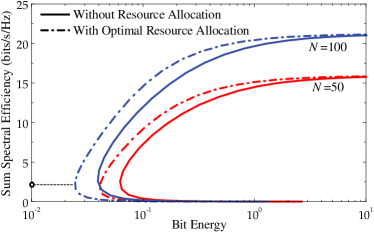
Figure 1: Bit energy versus sum spectral efficiency with and without resource allocation.

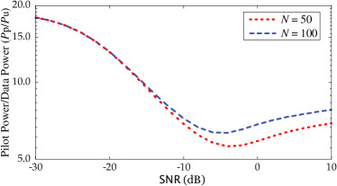
Figure 2: Ratio of the transmit pilot power to the transmit data power.

Proposition 1

The optimal pilot duration, $\tau$, of $\mathcal{P}_{1}$ is equal to the number of terminals $K$.

Proof:

Let $\left(\tau^{\ast},p_{\mathrm{p}}^{\ast},p_{\mathrm{u}}^{\ast}\right)$ be a solution of $\mathcal{P}_{1}$. Assume that $\tau^{\ast}>K$. Next we choose $\bar{\tau}=K$, $\bar{p}_{\mathrm{p}}=\tau^{\ast}p_{\mathrm{p}}^{\ast}/K$, and $\bar{p}_{\mathrm{u}}=\frac{P-\tau^{\ast}p_{\mathrm{p}}^{\ast}}{T-K}$. Clearly, this choice of system parameters $\left(\bar{\tau},\bar{p}_{\mathrm{p}},\bar{p}_{\mathrm{u}}\right)$ satisfies the constraints in (15). From (6) and using the fact that $\bar{\tau}\bar{p}_{\mathrm{p}}=\tau^{\ast}p_{\mathrm{p}}^{\ast}$, we have $\mathcal{S}\left(\bar{\tau},\bar{p}_{\mathrm{p}},\bar{p}_{\mathrm{u}}\right)>\mathcal{S}\left(\tau^{\ast},p_{\mathrm{p}}^{\ast},p_{\mathrm{u}}^{\ast}\right)$ which contradicts the assumption. Therefore, $\tau^{\ast}=K$. ∎

From Proposition 1, $\mathcal{P}_{1}$ is equivalent to the following optimization problem:

$$\mathcal{P}_{2}:\left\{\begin{array}[]{l}\mathop{\max}\limits_{p_{\mathrm{u}}}~{}\mathcal{S}|_{p_{\mathrm{p}}=P/K-(T/K-1)p_{\mathrm{u}}}\\ \hskip 8.5359pt\text{s.t.}~{}~{}0\leq p_{\mathrm{u}}\leq\frac{P}{T-K}.\\ \end{array}\right.$$ (18)

We can efficiently solve $\mathcal{P}_{2}$ based on the following property:

Proposition 2

The program $\mathcal{P}_{2}$ is concave.

Proof:

See Appendix -A. ∎

To solve the optimization problem $\mathcal{P}_{2}$, we can use any nonlinear or convex optimization method to get the globally optimal result. Here, we use the FMINCON function in MATLAB’s optimization toolbox.

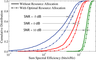
Figure 3: Sum spectral efficiency with and without resource allocation ($N=100$).

IV Numerical Results

We consider a cellular network with $L=7$ hexagonal cells which have a radius of $r_{c}=1000$m. Each cell serves $10$ terminals ($K=10$). We choose $T=200$, corresponding to a coherence bandwidth of $200$ KHz and a coherence time of $1$ ms. We consider the performance in the cell in the center of the network. We assume that terminals are located uniformly and randomly in each cell and no terminal is closer to the BS than $r_{h}=200$m. Large-scale fading is modeled as $\beta_{\ell ik}=z_{\ell ik}/(r_{\ell ik}/r_{h})^{\nu}$, where $z_{\ell ik}$ is a log-normal random variable, $r_{\ell ik}$ denotes the distance between the $k$th terminal in the $i$th cell and the $\ell$th BS, and $\nu$ is the path loss exponent. We set the standard deviation of $z_{\ell ik}$ to $8$dB, and $\nu=3.8$.

Firstly, we will examine the sum spectral efficiency versus the bit energy obtained from one snapshot generated by the above large-scale fading model. The bit energy is defined in (9). From (9) and (15), we can see that the solution of $\mathcal{P}_{1}$ also leads to the minimum value of the bit energy. Figure 1 presents the sum spectral efficiency versus the bit energy with optimal resource allocation. As discussed in Section II-C, the minimum bit energy is achieved at a non-zero spectral efficiency. For example, with optimal resource allocation, at $N=100$, the minimum bit energy is achieved at a sum spectral efficiency of $2$ bits/s/Hz which is marked by a circle in the figure. Below this value, the bit energy increases as the sum spectral efficiency decreases. For a given energy per bit, there are two operating points. Operating below the sum spectral efficiency, at which the minimum energy per bit is obtained, should be avoided.

On a different note, we can see that with optimal resource allocation, the system performance improves significantly. For example, to achieve the same sum spectral efficiency of $10$ bits/s/Hz, optimal resource allocation can improve the energy efficiencies by factors of $1.45$ and $1.5$ compared to the case of no resource allocation with $N=50$ and $N=100$, respectively. This dramatic increase underscores the importance of resource allocation in massive MIMO. However, at high bit energy, the squaring effect for the case of no resource allocation disappears and, hence, the advantages of resource allocation diminish. Furthermore, for the same sum spectral efficiency, $\mathcal{S}=10$ bits/s/Hz, and with resource allocation, by doubling the number of BS antennas from $50$ to $100$, we can improve the energy efficiency by a factor of $2.2$.

The corresponding ratio of the optimal pilot power to the optimal transmitted data power for $N=50$ and $N=100$ is shown in Fig. 2. Here, we define $\mathsf{SNR}\triangleq P/T$. Since $P$ is the total transmit energy spent in a coherence interval $T$ and the noise variance is $1$, $\mathsf{SNR}$ has the interpretation of average transmit SNR and is therefore dimensionless. We can see that at low $\mathsf{SNR}$ (or low spectral efficiency), we spend more power during the training phase, and vice versa at high $\mathsf{SNR}$. At low $\mathsf{SNR}$, $p_{\mathrm{p}}/p_{\mathrm{u}}\approx 18$ which leads to $\tau p_{\mathrm{p}}/{(T-\tau)p_{\mathrm{u}}}\approx 1$. This means that half of the total energy is used for uplink training and the other half is used for data transmission. Note that the power allocation problem in the low SNR regime is useful since the achievable rate (obtained under the assumption that the estimation error is additive Gaussian noise) is very tight, due to the use of Jensen’s bound in [5]. Furthermore, in general, the ratio of the optimal pilot power to the optimal data power does not always monotonically decrease with increasing $\mathsf{SNR}$. We can see from the figure that, when $\mathsf{SNR}$ is around $-5$dB, $p_{\mathrm{p}}/p_{\mathrm{u}}$ increases when $\mathsf{SNR}$ increases.

We now consider the cumulative distribution of the sum spectral efficiency obtained from $2000$ snapshots of large-scale fading (c.f. Fig. 3). As expected, our resource allocation improves the system performance substantially, especially at low SNR. More importantly, with resource allocation, the sum spectral efficiencies are more concentrated around their means compared to the case of no resource allocation. For example, at $\mathsf{SNR}=0$dB, resource allocation increases the $0.95$-likely sum spectral efficiency by a factor of $2$ compared to the case of no resource allocation.

V Conclusion

Conventionally, in massive MIMO, the transmit powers of the pilot signal and data payload signal are assumed to be equal. In this paper, we have posed and answered a basic question about the operation of massive MIMO: How much would the performance improve if the relative energy of the pilot waveform, compared to that of the payload waveform, were chosen optimally? The partitioning of time, or equivalently bandwidth, between pilots and data within a coherence interval was also optimally selected. We found that, with $100$ antennas at the BS, by optimally allocating energy to pilots, the energy efficiency can be increased as much as $50\%$, when each terminal has a throughput of about $1$ bit/s/Hz. Typically, when the SNR is low (e.g., around $-15$dB), at the optimum, the transmit power is then about $10$ times higher during the training phase than during the data transmission phase.

-A Proof of Proposition 2

From (6) and (18), the problem $\mathcal{P}_{2}$ becomes

$$\mathcal{P}_{2}=\left\{\begin{array}[]{l}\arg\mathop{\max}\limits_{p_{\mathrm{u}}}~{}\left(1-\frac{K}{T}\right)\sum_{k=1}^{K}\log_{2}\left(1+f_{k}\left(p_{\mathrm{u}}\right)\right)\\ \hskip 48.36958pt0\leq p_{\mathrm{u}}\leq\frac{P}{T-K}\\ \end{array}\right.$$ (21)

where

$$f_{k}\left(p_{\mathrm{u}}\right)$$

$$\triangleq\frac{a_{k}\left(P-\left(T-K\right)p_{\mathrm{u}}\right)p_{\mathrm{u}}}{b_{k}\left(P\!-\!\left(T\!-\!K\right)p_{\mathrm{u}}\right)p_{\mathrm{u}}+c_{k}p_{\mathrm{u}}+d_{k}\left(P\!-\!\left(T\!-\!K\right)p_{\mathrm{u}}\right)+1}$$

$$=\!\frac{a_{k}}{b_{k}}\!-\!\frac{a_{k}}{b_{k}}\frac{c_{k}p_{\mathrm{u}}+d_{k}\left(P-\left(T-K\right)p_{\mathrm{u}}\right)+1}{b_{k}\!\left(\!P\!\!-\!\left(\!T\!\!-\!K\!\right)p_{\mathrm{u}}\!\right)p_{\mathrm{u}}\!+\!c_{k}p_{\mathrm{u}}\!+\!d_{k}\!\left(\!P\!\!-\!\left(\!T\!\!-\!K\!\right)p_{\mathrm{u}}\!\right)\!+\!1}.$$

The second derivative of $f_{k}\left(p_{\mathrm{u}}\right)$ can be expressed as:

$$\omega_{k}\frac{\partial^{2}f_{k}\left(p_{\mathrm{u}}\right)}{\partial p_{\mathrm{u}}^{2}}=-b_{k}\hat{T}^{2}(c_{k}-d_{k}\hat{T})p_{\mathrm{u}}^{3}-3b_{k}\hat{T}^{2}(d_{k}P+1)p_{\mathrm{u}}^{2}$$

$$+3b_{k}\hat{T}P(d_{k}P+1)p_{\mathrm{u}}-(d_{k}P+1)(b_{k}P^{2}+c_{k}P+\hat{T}),$$ (22)

where $\omega_{k}\triangleq\frac{\left(b_{k}\left(P\!-\!\hat{T}p_{\mathrm{u}}\right)p_{\mathrm{u}}+c_{k}p_{\mathrm{u}}+d_{k}\left(P\!-\!\hat{T}p_{\mathrm{u}}\right)+1\right)^{3}}{2a_{k}}$, and $\hat{T}\triangleq T-K$. Since $P\geq\hat{T}p_{\mathrm{u}}$, we have

$$\omega_{k}\frac{\partial^{2}f_{k}\left(p_{\mathrm{u}}\right)}{\partial p_{\mathrm{u}}^{2}}=-b_{k}c_{k}\hat{T}^{2}p_{\mathrm{u}}^{3}-(d_{k}P+1)(c_{k}P+\hat{T})$$

$$-\frac{3}{4}b_{k}\hat{T}^{2}p_{\mathrm{u}}^{2}-b_{k}\left(P-\frac{3}{2}\hat{T}p_{\mathrm{u}}\right)^{2}-b_{k}d_{k}(P-\hat{T}p_{\mathrm{u}})^{3}\leq 0.$$ (23)

Since $\omega_{k}>0$, $\frac{\partial^{2}f_{k}\left(p_{\mathrm{u}}\right)}{\partial p_{\mathrm{u}}^{2}}\leq 0$. Therefore, $f_{k}\left(p_{\mathrm{u}}\right)$ is a concave function in $0\leq p_{\mathrm{u}}\leq\frac{P}{T-K}$. Since $\log_{2}\left(1+x\right)$ is a concave and increasing function, $\log_{2}\left(1+f_{k}\left(p_{\mathrm{u}}\right)\right)$ is also a concave function. Finally, using the fact that the summation of concave functions is concave, we conclude the proof of Proposition 2.

References

- [1] T. L. Marzetta, “Noncooperative cellular wireless with unlimited numbers of base station antennas,” IEEE Trans. Wireless Commun., vol. 9, no. 11, pp. 3590–3600, Nov. 2010.
- [2] E. G. Larsson, F. Tufvesson, O. Edfors, and T. L. Marzetta, “Massive MIMO for next generation wireless systems,” IEEE Commun. Mag., vol. 52, no. 2, pp. 186–195, Feb. 2014.
- [3] H. Yin, D. Gesbert, M. Filippou, and Y. Liu, “A coordinated approach to channel estimation in large-scale multiple-antenna systems,” IEEE J. Sel. Areas Commun., vol. 31, no. 2, pp. 264–273, Feb. 2013.
- [4] K. T. Truong and R. W. Heath Jr., “Effects of channel aging in massive MIMO systems,” IEEE J. Commun. Netw., vol. 15, no. 4, pp. 338–351, Aug. 2013.
- [5] H. Q. Ngo, E. G. Larsson, and T. L. Marzetta, “Energy and spectral efficiency of very large multiuser MIMO systems,” IEEE Trans. Commun., vol. 61, no. 4, pp. 1436–1449, Apr. 2013.
- [6] B. Hassibi and B. M. Hochwald, “How much training is needed in multiple-antenna wireless links?” IEEE Trans. Inf. Theory, vol. 49, no. 4, pp. 951–963, Apr. 2003.
- [7] V. Raghavan, G. Hariharan, and A. M. Sayeed, “Capacity of sparse multipath channels in the ultra-wideband regime,” IEEE J. Sel. Topics Signal Process., vol. 1, no. 5, pp. 357-371, Oct. 2007.
- [8] S. Murugesan, E. Uysal-Biyikoglu, and P. Schniter, “Optimization of training and scheduling in the non-coherent SIMO multiple access channel,” IEEE J. Sel. Areas Commun., vol. 25, no. 7, pp. 1446–1456, Sep. 2007.
- [9] S. Verdú, “Spectral efficiency in the wideband regime,” IEEE Trans. Inf. Theory, vol. 48, no. 6, pp. 1319-1343, June 2002.