Conformal field theories at non-zero temperature:
operator product expansions, Monte Carlo, and holography

Abstract

We compute the non-zero temperature conductivity of conserved flavor currents in conformal field theories (CFTs) in 2+1 spacetime dimensions. At frequencies much greater than the temperature, $\hbar\omega\gg k_{B}T$, the $\omega$ dependence can be computed from the operator product expansion (OPE) between the currents and operators which acquire a non-zero expectation value at $T>0$. Such results are found to be in excellent agreement with quantum Monte Carlo studies of the O(2) Wilson-Fisher CFT. Results for the conductivity and other observables are also obtained in vector $1/N$ expansions. We match these large $\omega$ results to the corresponding correlators of holographic representations of the CFT: the holographic approach then allows us to extrapolate to small $\hbar\omega/(k_{B}T)$. Other holographic studies implicitly only used the OPE between the currents and the energy-momentum tensor, and this yields the correct leading large $\omega$ behavior for a large class of CFTs. However, for the Wilson-Fisher CFT a relevant “thermal” operator must also be considered, and then consistency with the Monte Carlo results is obtained without a previously needed ad hoc rescaling of the $T$ value. We also establish sum rules obeyed by the conductivity of a wide class of CFTs.

I Introduction

Conformal field theories (CFTs) constitute the best characterized quantum systems without quasiparticle excitations. Their non-zero temperature dissipative dynamics can be treated by extensions of Boltzmann-like approaches designed for quasiparticle dynamics Damle and Sachdev (1997); the Boltzmann approach is difficult in general, thus limited in practice. Much additional insight can be gained from a modern perspective based upon holographic ideas Witczak-Krempa et al. (2014), which does not assume a quasiparticle decomposition of the spectrum at any stage. CFTs are also important as models of quantum critical points in condensed matter, notably for the superfluid-insulator transition of bosons in a periodic potential in two spatial dimensions Spielman et al. (2007); Zhang et al. (2012); Endres et al. (2012).

In recent work by three of us Witczak-Krempa et al. (2014), we computed the $T>0$ conductivity of a lattice model for this superfluid-insulator transition using quantum Monte Carlo simulations; after carefully taking the $T\rightarrow 0$ limit of the lattice model, we obtained the $T>0$ conductivity of a conserved current of the CFT, and this was compared with the predictions of a semi-phenomenological holographic theory. The latter theory included terms up to four derivatives in the metric and a gauge field conjugate to the conserved current. We found consistency between the two approaches after an ad hoc rescaling of the temperature between the two methods. Related $T>0$ results were obtained in Refs. Šmakov and Sørensen, 2005; Chen et al., 2014, $T=0$ results are in Refs. Gazit et al., 2013, 2014, and the effects of disorder were considered in Refs. Lin et al., 2011; Swanson et al., 2014.

The present paper will significantly improve on our previous analysis by using more specific field-theoretic information on the CFTs under consideration. We will work mainly with the 2+1 dimensional CFT with O($N$) symmetry described by the Wilson-Fisher fixed point, and determine the conductivity of the conserved O($N$) current. We will compute the operator product expansion (OPE) of the current operators in terms of other operators of the CFT, and use this to constrain the high frequency behavior of the conductivity. We find excellent agreement of such results with Monte Carlo studies of the O(2) model upon taking into account a scalar field conjugate to a relevant perturbation of the CFT. Next, we will connect the high frequency behavior to holography, and use it to make predictions for the conductivity at lower frequencies without an ad hoc rescaling of temperature.

From a broader perspective, our analysis shows how the finite temperature properties of CFTs can be analyzed by systematically including the influence of low dimension operators to constrain the short-time behavior, and then using holography to extrapolate to longer times. In theories with quasiparticles, the extrapolation from short to long times is generally made via the Boltzmann equation; here, we argue that the corresponding extrapolation for CFTs without quasiparticles can be made by a combination of the OPE with holography.

We present here the structure of the high frequency, or short time, behavior of the conductivity as given by the OPE for a general CFT in 2+1 dimensions. With spacetime co-ordinates $(\tau,x,y)$, the conductivity is related to the two-point correlator of a conserved current $J_{x}$ (we suppress indices of global flavor symmetries). We work in the Euclidean time signature, and then the conductivity is

$$\frac{\sigma(i\omega_{n})}{\sigma_{Q}}=-\frac{1}{\omega_{n}}\left\langle J_{x}({\bm{\omega}})J_{x}(-{\bm{\omega}})\right\rangle_{T}+\mbox{a possible contact term}\,,$$ (1)

where ${\bm{\omega}}\equiv(\omega_{n},0,0)$, and in some cases a diamagnetic “contact” term may be present (this is the case for the O$(N)$ model); here $\omega_{n}$ refers to Matsubara frequencies which are integral multiples of $2\pi T$, but the conductivity is defined at all $\omega$ by analytic continuation. To make contact with the condensed matter literature, we have explicitly displayed a factor of the quantum unit of conductance

$$\sigma_{Q}=\frac{(e^{\ast})^{2}}{\hbar}\,,$$ (2)

where $e^{\ast}$ is the effective charge of the carriers ($e^{\ast}=2e$ for the superfluid-insulator transition of Cooper pairs); the ratio $\sigma/\sigma_{Q}$ is then a dimensionless function whose values we will present here. Note that, in the condensed matter literature $(e^{\ast})^{2}/h=2\pi\sigma_{Q}$ is often used as a definition of the quantum unit of conductance.

The OPE specifies the behavior of the product of a pair of operators when they approach the same point in spacetime: the product is replaced by a sum over the operators of the CFT with universal coefficients El-Showk et al. (2012); Pappadopulo et al. (2012). These OPE coefficients ultimately allow one to compute all local correlators of the CFT at $T=0$. At $T>0$, the OPE expansion is applicable for times $|t|<\hbar/(k_{B}T)$ (we will set $\hbar=k_{B}=1$ in subsequent expressions), but cannot be used directly for longer times which are naturally sensitive to the global topology of spacetime, and in particular to the periodic boundary conditions along the Euclidean temporal direction. For our purposes, it is useful to work in frequency space, and to express the OPE as the product of 2 operators when they carry a common large Euclidean frequency. One of our primary results is the following OPE of the product of 2 currents

$$\lim_{|\Omega|\gg p}J_{x}({\bm{\omega}})J_{x}(-{\bm{\omega}}+{\bm{p}}) = -|\Omega|\,\sigma_{\infty}\,\delta^{(3)}({\bm{p}})-\frac{\mathcal{C}}{|\Omega|^{\Delta-1}}\mathcal{O}({\bm{p}})$$ (3)

$$~{}+\frac{\mathcal{C}_{T}}{\Omega^{2}}\Bigl{[}T_{xx}({\bm{p}})-T_{yy}({\bm{p}})-12\gamma(T_{xx}({\bm{p}})+T_{yy}({\bm{p}}))\Bigr{]}+\dotsb,$$

where ${\bm{\omega}}\equiv(\Omega,0,0)$, with $\Omega$ being the imaginary frequency at $T=0$, and ${\bm{p}}$ is a fixed 3-momentum with $p\equiv|{\bm{p}}|$. The structure of this OPE was deduced by computing correlators of the operators on the left-hand-side with those on the right-hand-side using the $1/N$ expansion of the O($N$) model; it is also consistent with correlators deduced from holography. Taking an expectation of the above equation at any temperature will lead to both sides being proportional to $\delta^{(3)}({\bm{p}})$. Here $\sigma_{\infty}$ is limiting value of the conductivity obtained as $T\rightarrow 0$, $\mathcal{O}$ is a possible scalar operator in the OPE with scaling dimension $\Delta$, $T_{\mu\nu}$ is the energy-momentum tensor, and $\mathcal{C}$, $\mathcal{C}_{T}$, and $\gamma$ are OPE coefficients.

The terms in Eq. (3) involving the energy-momentum tensor have been implicitly included in previous studies Myers et al. (2011); Chowdhury et al. (2013); Witczak-Krempa et al. (2014). In the holographic approach, these terms arise from the coupling, $\gamma$, of the Weyl tensor to the gauge flux Ritz and Ward (2009); Myers et al. (2011); the value of $\gamma$ obeys the exact bound Myers et al. (2011); Chowdhury et al. (2013) $|\gamma|\leq 1/12$. It is also interesting to note the resemblance of the energy-momentum terms in Eq. (3) to the Sugawara construction Sugawara (1968); Goddard et al. (1985) of the energy-momentum tensor from the OPE of currents in CFTs in 1+1 dimension; indeed, the term proportional to $\gamma$ is $T_{xx}+T_{yy}=-T_{\tau\tau}$, the Hamiltonian density.

We can use Eq. (3) to determine the frequency dependence of the conductivity at finite temperature in the regime $\hbar|\omega_{n}|\gg k_{B}T$, where $\omega_{n}$ is the Matsubara frequency (we will henceforth set $\hbar=k_{B}=1$). We simply evaluate the expectation value of the right-hand-side in an equilibrium thermal ensemble defined by the CFT, and indeed we have only displayed terms in Eq. (3) which have a non-zero expectation value at $T>0$. By this method we obtain from Eqs. (1) and (3)

$$\frac{\sigma(i\omega_{n})}{\sigma_{Q}}=\sigma_{\infty}+b_{1}\,\left(\frac{T}{\omega_{n}}\right)^{\Delta}+b_{2}\,\left(\frac{T}{\omega_{n}}\right)^{3}+\dotsb,\quad\quad\omega_{n}\gg T\,,$$ (4)

where the dimensionless numbers $b_{1}$, $b_{2}$ are related to the OPE coefficients $\mathcal{C}$ and $\mathcal{C}_{T}$ respectively. This expression shows that the term associated with the operator $\mathcal{O}$ is important when there is a scalar operator with a scaling dimension $\Delta<3$. For the O($N$) Wilson-Fisher CFT there is indeed such an operator: it is the “thermal” operator $\mathcal{O}_{g}$, whose introduction breaks no symmetry and drives the CFT into a non-critical state. We note that the label “thermal” descends from critical phenomena terminology, and is not meant to imply that $\mathcal{O}_{g}$ introduces a non-zero $T$; such an operator has a coupling $g$ in the action, and $g$ has to be tuned to a critical value $g=g_{c}$ to realize the CFT. The operator $\mathcal{O}_{g}$ has scaling dimension $\Delta$ which takes the value

$$\Delta_{g}=3-1/\nu\,,$$ (5)

where $\nu$ is the correlation length exponent. For $N=2$, we have $\nu\approx 2/3$, and so the $\mathcal{O}=\mathcal{O}_{g}$ term in Eqs. (3) and (4) is more important than that due to the energy-momentum tensor, at least at large $\omega_{n}$.

The previous analysis Witczak-Krempa et al. (2014) did not allow for an operator $\mathcal{O}$ with $\Delta<3$. Indeed, there is no such operator for numerous physically interesting CFTs involving Dirac fermions coupled to gauge fields, including QED3. For these CFTs, the analysis of Ref. Witczak-Krempa et al. (2014) can be used without modification. However, for O($N$) Wilson-Fisher CFT, it is necessary to extend the analysis to include the relevant operator $\mathcal{O}_{g}$; such an extension was briefly noted in Ref. Witczak-Krempa and Sachdev, 2012, but its consequences were not appropriately analyzed. After such an extension here, we find excellent compatibility between Monte Carlo, operator product expansions, and holography, without any ad hoc rescaling of temperature.

We will begin our analysis by computations in the vector $1/N$ expansion for the O($N$) Wilson-Fisher CFT in Section II. With many details relegated to the Appendix, we obtain results for OPE coefficients and thermal expectation values. Section III presents our Monte Carlo results on the $N=2$ Wilson-Fisher CFT, and compares them with the $1/N$ expansion. Section IV turns to holography: by matching the large frequency behavior with the Monte Carlo results, we are able to extrapolate to low frequency properties of the conductivity. Section V presents a few results for CFTs with Dirac fermions. Finally, in Section VI we use the OPE analysis to prove conductivity sum rules.

We close this introduction by summarizing our notations for the operators under consideration in Table 1, as they appear in Sections II-IV.

$\mathcal{O}$	$\Delta_{\mathcal{O}}$	$\;\ell\;$	$\left\langle\mathcal{O}\right\rangle_{T}$	Holographic dual
$\phi_{\alpha}$	$(1+\eta)/2$	0	0	$-$
$\mathcal{O}_{g}\sim\phi_{\alpha}^{2}$	$3-1/\nu$	0	$BT^{3-1/\nu}$	$\varphi$
$J_{\mu}$	2	1	0	$A_{\mu}$
$T_{\mu\nu}$	3	2	$H_{\mu\nu}T^{3}$	$g_{\mu\nu}$

Table 1: Main operators of the CFT describing the O$(N)$ Wilson-Fisher CFT in 2+1 dimensions. $\Delta_{\mathcal{O}},\ell$ are the scaling dimension and spin of the operators, respectively. The properties of the conserved current $J_{\mu}$ (with flavor index suppressed) and energy-momentum tensor $T_{\mu\nu}$ are general for any CFT in 2+1 dimensions.

II O($N$) CFT

The theory of primary interest to us is described by the partition function for a O$(N)$ vector field $\phi_{\alpha}$, $\alpha=1,\dotsc,N$,

$$Z=\int\mathcal{D}\phi_{\alpha}\exp\left(-\int_{\bm{x}}\left[\frac{1}{2}(\partial\phi_{\alpha})^{2}+\frac{v}{2N}\left(\phi_{\alpha}^{2}-N/g\right)^{2}\right]\right)\,,$$ (6)

where $\int_{\bm{x}}\equiv\int d^{3}x$ is the integral over 2+1 dimensional spacetime, $v$ parametrizes the quartic non-linearity, and $g$ is the tuning parameter across a quantum phase transition between phases where O($N$) symmetry is broken and present. We have written this field theory in a somewhat unconventional notation to facilitate a $1/N$ expansion; to the extent possible, we follow the notation in Ref. Podolsky and Sachdev (2012). In the limit $v\rightarrow\infty$ this theory reduces to the O($N$) non-linear sigma model. However, it is a subtle matter to identify the thermal operator in the strict $v=\infty$ theory, as was discussed in Ref. Podolsky and Sachdev (2012). We will therefore keep $v$ finite for now, but will shortly indeed take the $v\rightarrow\infty$ limit when it no longer interferes with the scaling limit.

We will primarily be interested in the conductivity of this theory at the quantum critical point $g=g_{c}$ as a function of frequency, $\omega$, and absolute temperature $T$. Without loss of generality, we focus on one of the conserved O($N$) currents of this theory,

$$J_{x}=\phi_{1}\partial_{x}\phi_{2}-\phi_{2}\partial_{x}\phi_{1}\,.$$ (7)

The computationally challenging regime is at low frequencies $|\omega|\ll T$, where we have the dissipative dynamics of the CFT relaxing to thermal equilibrium. However, controlled and reliable studies are possible at high frequencies $\omega\gg T$. In this section, we will present the results of a $1/N$ expansion of the behavior of the conductivity in this $\omega\gg T$ regime using the OPE in Eq. (3).

The leading term in Eq. (3) is given by the constant $\sigma_{\infty}$ which has been computed earlier. For completeness, we note its value in the $1/N$ expansion Cha et al. (1991); Huh et al. (2013) for the theory $Z$

$$\sigma_{\infty}=\frac{1}{16}\left(1-\frac{1}{N}\frac{64}{9\pi^{2}}+\mathcal{O}(1/N^{2})\right).$$ (8)

The terms in Eq. (3) involving the energy-momentum tensor have been discussed previously in different formulations Myers et al. (2011); Chowdhury et al. (2013); Witczak-Krempa et al. (2014). We can use holography to compute the 3-point correlator between $J_{x}$, $J_{x}$, and $T_{\mu\nu}$ as described in Ref. Chowdhury et al. (2013), and then deduce the structure of the OPE: this computation in described in Appendix A. We can also compute the same 3-point correlator in the $1/N$ expansion as described in Ref. Chowdhury et al. (2013), and again obtain Eq. (3) with specific values of the OPE coefficients: this is also described in Appendix A. The $1/N$ expansion for $\gamma$ for the theory $Z$ is Chowdhury et al. (2013)

$$\gamma=-\frac{1}{12}+\mathcal{O}(1/N)\,.$$ (9)

Similarly, the $1/N$ expansion for $\mathcal{C}_{T}$ is

$$\mathcal{C}_{T}=\frac{4}{N}+\mathcal{O}(1/N^{2})\,.$$ (10)

For the O($N$) field theory in Eq. (6), there is a relevant scalar operator $\mathcal{O}$ which we denote $\mathcal{O}_{g}$ because it is generated by tuning $g$ away from the quantum critical point. This is the operator $\mathcal{O}_{g}\sim\phi_{\alpha}^{2}$ with scaling dimension in Eq. (5).

We will compute the OPE coefficient of $\mathcal{O}_{g}$ in the $1/N$ expansion of $Z$. An important subtlety arises in the definition of $\mathcal{O}_{g}$ in such an expansion, as we now describe. The scaling limit of the large $N$ expansion also involves taking the limit Brézin and Zinn-Justin (1976) $v\rightarrow\infty$ in the action in Eq. (6). However, in this limit, we see from Eq. (6) that $\phi_{\alpha}^{2}=N/g$, a constant. Consequently, the correspondence $\mathcal{O}_{g}\sim\phi_{\alpha}^{2}$, assumed in Ref. Witczak-Krempa and Sachdev, 2012, does not define an appropriate non-constant thermal operator at $v=\infty$. A proper definition of $\mathcal{O}_{g}$ requires a more careful analysis of the $N\rightarrow\infty$ and $v\rightarrow\infty$ limits Podolsky and Sachdev (2012). We decouple the quartic term in $Z$ by a Hubbard-Stratonovich field $\widetilde{\lambda}$ and write

$$Z=\int\mathcal{D}\phi_{\alpha}\mathcal{D}\widetilde{\lambda}\exp\left(-\frac{1}{2}\int_{\bm{x}}\left[\left(\partial\phi_{\alpha}\right)^{2}+\frac{i}{\sqrt{N}}\widetilde{\lambda}\left(\phi_{\alpha}^{2}-N/g\right)+\frac{\widetilde{\lambda}^{2}}{4v}\right]\right)\,.$$ (11)

It is the field $i\widetilde{\lambda}$ which we will identify with the operator $\mathcal{O}_{g}$. This identification is motivated by the following identities between the one- and two-point correlators of $\phi_{\alpha}^{2}$ and $\widetilde{\lambda}$ (which can be obtained by taking appropriate functional derivatives of source terms) Podolsky and Sachdev (2012)

$$\left\langle\phi_{\alpha}^{2}({\bm{x}})\right\rangle = \frac{N}{g}+i\frac{\sqrt{N}}{2v}\left\langle\widetilde{\lambda}({\bm{x}})\right\rangle\,;$$

$$\left\langle\phi_{\alpha}^{2}({\bm{x}})\phi_{\beta}^{2}(0)\right\rangle-\left\langle\phi_{\alpha}^{2}(0)\right\rangle^{2} = \frac{N}{v}\delta^{(3)}({\bm{x}})-\frac{N}{4v^{2}}\left[\left\langle\widetilde{\lambda}({\bm{x}})\widetilde{\lambda}(0)\right\rangle-\left\langle\widetilde{\lambda}(0)\right\rangle^{2}\right].$$ (12)

So up to unimportant additive terms, the correlators of $\phi_{\alpha}^{2}$ are equal to those of $(\sqrt{N}/(2v))i\widetilde{\lambda}$. As reviewed in Ref. Podolsky and Sachdev (2012), the correlators of $i\widetilde{\lambda}$ have a sensible scaling limit in a theory in which we take the $v\rightarrow\infty$ limit already in the action in Eq. (11). So we identify $\mathcal{O}_{g}\sim i\widetilde{\lambda}$, and then set $v=\infty$ in subsequent computations. Note, however, that Eqs. (12) become trivial at $v=\infty$, and so $v$ has to be kept finite only in deducing the correlators of $\phi_{\alpha}^{2}$. Specifically, we define the “thermal” operator by

$$\mathcal{O}_{g}({\bm{x}})=C_{\lambda}\,i\widetilde{\lambda}({\bm{x}})\,,$$ (13)

where the cutoff-dependent constant $C_{\lambda}$ will be chosen so that the two-point correlator of $\mathcal{O}_{g}$ is normalized as

$$\left\langle\mathcal{O}_{g}({\bm{p}})\mathcal{O}_{g}(-{\bm{p}})\right\rangle-\left\langle\mathcal{O}_{g}\right\rangle^{2}=-16p^{3-2/\nu}.$$ (14)

The pre-factor of 16 is chosen for convenience in the $1/N$ expansion: we find in Appendix B that $C_{\lambda}=1$ at $N=\infty$. With these definitions and normalizations, we can compute the value of the OPE coefficient $\mathcal{C}_{g}$: we find in Appendix B that

$$\mathcal{C}_{g}=\frac{1}{4\sqrt{N}}+\mathcal{O}(1/N^{3/2})\,.$$ (15)

With all the ingredients in the OPE at hand, we can proceed to the determination of $T>0$ behavior of the conductivity from Eq. (3). For this, we need the expectation values of $\mathcal{O}_{g}$ and $T_{\mu\nu}$ at $T>0$: these are determined in Appendix C.

For the operator $\mathcal{O}_{g}$ we obtain

$$\left\langle\mathcal{O}_{g}\right\rangle_{T}-\left\langle\mathcal{O}_{g}\right\rangle_{T=0}\equiv BT^{3-1/\nu}$$ (16)

with

$$B=\sqrt{N}\Theta^{2}\left[1-\frac{1.8914}{N}+\mathcal{O}(1/N^{2})\right],$$ (17)

where

$$\Theta\equiv 2\ln\left(\frac{\sqrt{5}+1}{2}\right).$$ (18)

In Eq. (16), we note that we have subtracted the $T=0$ expectation value, which is non-universal and finite in the field theory Eq. (6). This subtraction can be seen as defining the scaling operator of the IR fixed point CFT, in which the expectation values at zero temperature vanish. For the purposes of comparing with our Monte Carlo results, it useful to express this result in a form that is independent of our arbitrary normalization of $\mathcal{O}_{g}$ in Eq. (14). We take the Fourier transform of Eq. (14) to real space to obtain

$$\left\langle\mathcal{O}_{g}({\bm{x}})\mathcal{O}_{g}(0)\right\rangle\equiv\frac{A}{x^{6-2/\nu}}$$ (19)

with

$$A=-\frac{2^{7-2/\nu}\Gamma(3-1/\nu)}{\pi^{3/2}\Gamma(-3/2+1/\nu)}\,.$$ (20)

From Eqs. (20) and (17) we can construct the universal ratio which is independent of the normalization convention of $\mathcal{O}_{g}$:

$$\Upsilon=\frac{\sqrt{A}}{B}=\frac{4}{\pi\Theta^{2}\sqrt{N}}\left[1+\frac{0.8941}{N}+\mathcal{O}(1/N^{2})\right].$$ (21)

This ratio will be compared with quantum Monte Carlo results for $N=2$ in Section III; its value will also be useful in the holographic analysis in Section IV.

For the $T>0$ expectation value of the energy-momentum tensor, we have for any CFT

$$\left\langle T_{xx}\right\rangle_{T}=\left\langle T_{yy}\right\rangle_{T}=-\frac{1}{2}\left\langle T_{\tau\tau}\right\rangle_{T}=H_{xx}T^{3}\,,$$ (22)

which corresponds to the pressure of the CFT. We have implicitly subtracted from these expectation values their $T=0$ value; $H_{xx}$ is a universal number characterizing the CFT. This equation manifestly shows the tracelessness of $T_{\mu\nu}$ in a CFT, which holds at finite temperature. The computation in Appendix C shows that in the large-$N$ limit of the O($N$) model

$$H_{xx}=\frac{\zeta(3)}{2\pi}\left(\frac{4N}{5}-0.3344\right)\,.$$ (23)

Collecting our results, we can now insert Eqs. (16) and (23) into Eq. (3) and obtain the large frequency behavior of the conductivity in the O($N$) CFT:

$$\frac{\sigma(i\omega_{n})}{\sigma_{Q}}=\sigma_{\infty}+\mathcal{C}_{g}\,B\,\left(\frac{T}{\omega_{n}}\right)^{3-1/\nu}+24\,\mathcal{C}_{T}\,\gamma\,H_{xx}\,\left(\frac{T}{\omega_{n}}\right)^{3}+\dotsb\,.$$ (24)

Note that this is the result for Euclidean frequencies $\omega_{n}\gg T$. We show in Appendix C that the result agrees precisely with explicit computation of the conductivity in the $N=\infty$ theory, which appears in Eq. (109). The result Eq. (24) shows that the combination $\mathcal{C}_{g}B$ is also independent of the normalization convention of $\mathcal{O}_{g}$.

The analytic continuation $i\omega_{n}\rightarrow\omega+i0^{+}$ of Eq. (24) to real frequencies $\omega\gg T$ yields:

$$\frac{\sigma(\omega/T)}{\sigma_{Q}}=\sigma_{\infty}+b_{1}\left[\operatorname{Re}(i^{\Delta_{g}})+i\operatorname{Im}(i^{\Delta_{g}})\right]\left(\frac{T}{\omega}\right)^{\Delta_{g}}-i\,b_{2}\left(\frac{T}{\omega}\right)^{3}+\dotsb,$$ (25)

where $\Delta_{g}=3-1/\nu$. We note that for finite $N>1$, the scaling dimension $\Delta_{g}$ is not an integer, making both the real and imaginary parts of $\sigma(\omega/T)$ to scale like $(T/\omega)^{\Delta_{g}}$ at large $\omega/T$. For instance if we set $\nu=2/3$, this yields $\Delta_{g}=3/2$, thus $\operatorname{Im}(i^{3/2})=-\operatorname{Re}(i^{3/2})=1/\sqrt{2}$. In contrast, the $N=\infty$ limit is special because $\Delta_{g}$ is an integer, 2, and thus only the real part scales like $(T/\omega)^{2}$, while the imaginary part decays faster, i.e. as $(T/\omega)^{3}$. In the case of CFTs that do not have a scalar operator with scaling dimension $\Delta<3$ in the $JJ$ OPE, the real and imaginary parts of the conductivity at asymptotically large and real frequencies behave differently. The imaginary parts decays as $(T/\omega)^{3}$ due to the energy-momentum tensor, while the real part decays faster due the presence of other operators. This is the case for certain CFTs involving Dirac fermions discussed in Section V. It is also the case for the holographic models previously considered Ritz and Ward (2009); Myers et al. (2011), as shown in Ref. Witczak-Krempa (2014).

III Quantum Monte Carlo

In order to perform efficient Quantum Monte Carlo simulations of Eq. (6) for $N=2$ it is useful to introduce a simple lattice model in the same universality class. For this purpose we use a quantum rotor model defined in terms of phases $\theta_{\vec{r}}$ living on the sites, $\vec{r}$, of a two-dimensional square lattice:

$$H_{\text{qr}}=\frac{U}{2}\sum_{\vec{r}}\frac{1}{2}\left(\frac{1}{i}\frac{\partial}{\partial\theta_{\vec{r}}}\right)^{2}-\mu\sum_{\vec{r}}\frac{1}{i}\frac{\partial}{\partial\theta_{\vec{r}}}-\sum_{\langle\vec{r},\vec{r}^{\prime}\rangle}t\cos(\theta_{\vec{r}}-\theta_{\vec{r}^{\prime}})\ .$$ (26)

Here $-i{\partial}/{\partial\theta_{\vec{r}}}$ is usually identified with the angular momentum of the quantum rotor at site ${\vec{r}}$, which is the canonical conjugate of $\theta_{\vec{r}}$. However, it can also be viewed as the deviation from an average (integer) particle number and this model is therefore in the same universality class as the Bose Hubbard model. The on-site repulsive interaction, $U$, then hinders large deviations from the mean particle number while $t$ characterizes the hopping between nearest neighbor sites. For completeness, we include a chemical potential $\mu$ although the case of integer filling that we focus on here corresponds to $\mu=0$.

As discussed in Ref. Witczak-Krempa et al., 2014, it is possible to directly simulate Eq. (26) using quantum Monte Carlo (QMC) techniques. However, it is useful to further simplify the model by employing the Villain approximation Villain (1975) where the $\cos\theta$ term is replaced by a sum of periodic Gaussians centered at $2\pi m$ (where $m$ is an integer): $\exp({t\Delta\tau\cos(\theta)})\simeq\exp({t\Delta\tau})\sum_{m}\exp({-\frac{1}{2}t\Delta\tau(\theta-2\pi m)^{2}}),$ preserving the periodicity of the Hamiltonian in $\theta$. A standard Trotter decomposition can then be performed where $\beta U$, is divided into $L_{\tau}$ slices of size $\Delta\tau=\beta U/L_{\tau}$. One then arrives at a model defined in terms of an integer-valued current ${\bf J}=(J^{\tau},J^{x},J^{y})$ with $J^{\tau}$ the angular momentum (or particle number) living on the links of a $2+1$ dimensional discrete lattice of dimensions $L\times L\times L_{\tau}$: Cha et al. (1991); Sørensen et al. (1992); Wallin et al. (1994)

$$Z_{V}\approx{\sum_{\{\bf J\}}}^{\prime}\exp\left[-\frac{1}{K}\sum_{(\tau,{\vec{r}})}\left(\frac{1}{2}{\bf J}^{2}_{(\tau,{\vec{r}})}-\frac{\mu}{U}J^{\tau}_{(\tau,{\vec{r}})}\right)\right]\ .$$ (27)

Here $L_{\tau}\Delta\tau$ takes the place of the dimensionless inverse temperature $\beta U$ and varying $K$ is analogous to varying $\sqrt{t/U}$ in the quantum rotor model. We stress that, the ${\sum}^{\prime}$ denotes the fact that the summation over ${\bf J}$ is constrained to divergence-less configurations making the summation over the integer valued currents highly non-trivial to perform. In deriving the Villain model a fixed $\Delta\tau=1/K$ is used. Despite the fixed, rather large, value of $\Delta\tau$, the Villain model has several significant advantages. Most notably, it is explicitly isotropic in space and time. Secondly, very efficient Monte Carlo algorithms have been developed for the Villain model Alet and Sørensen (2003a, b) as well as for the quantum rotor model. Here we use directed Monte Carlo techniques as described in Ref. Alet and Sørensen, 2003b. The location of the QCP is also known, $K_{c}=0.3330671(5)$. Chen et al. (2014); Witczak-Krempa et al. (2014) Further details of the numerical calculations are given in Appendix D.

In the condensed matter literature the quantum of conductance is usually defined as $(e^{*})^{2}/h$ (for carriers of charge $e^{*}$), however, here we use a slightly different definition of $\sigma_{Q}=(e^{*})^{2}/\hbar$ that is also widely used. In terms of $\sigma_{Q}$, the frequency dependent conductivity of the Villain model can then be calculated by evaluating ($\omega_{n}$ are the Matsubara Euclidean frequencies)

$$\frac{\sigma(i\omega_{n})}{\sigma_{Q}}=\frac{1}{L^{d-2}2\pi n}\left\langle\left|\frac{1}{L}\sum_{(\tau,{\vec{r}})}e^{i\omega_{n}\tau}J^{x}_{(\tau,{\vec{r}})}\right|^{2}\right\rangle\,,$$ (28)

which is dimensionless in $d=2$. Here $n$ is an integer labeling the (dimensionless) Matsubara frequency $\omega_{n}/\omega_{c}=2\pi n/L_{\tau}$. We note that this expression is explicitly independent of the imaginary time discretization $\Delta\tau$ even though $\omega_{n}$ is measured in units of $\omega_{c}=U/\Delta\tau$ and any residual dependence of $\sigma(i\omega_{n})$ on $\Delta\tau$ is therefore usually ignored.

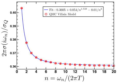
Figure 1: QMC results (open circles) at $K_{c}=0.3330671$ with $\mu=0$ for the frequency dependent conductivity $\sigma(i\omega_{n})$. All results have first been extrapolated to $L\to\infty$ and subsequently to $T\to 0$ ($L_{\tau}\to\infty$). The solid blue line shows a fit to the QMC data for $n=1,\ldots,7$ of the form $2\pi\sigma/\sigma_{Q}=0.3605+0.054/n^{1.533}-0.01/n^{3}$ with $n=\omega_{n}/(2\pi T)$ the Matsubara index. The dashed blue line is the continuation of the fitted form to $n>7$.

The conductivity at the QCP has previously been studied Cha et al. (1991); Sørensen et al. (1992); Wallin et al. (1994). The first attempts at calculating the universal $T\to 0$ limit of the conductivity Šmakov and Sørensen (2005) appeared significantly later and the first large scale numerical calculations of this quantity have only very recently been performed Witczak-Krempa et al. (2014); Chen et al. (2014) due to their extremely demanding nature. Here we re-analyze the numerical results of Ref. Witczak-Krempa et al., 2014 in order to test the analytical result, Eqs. (4) and (24). The $T\to 0$ extrapolated QMC results for the conductivity are shown in Fig. 1 along with our fit. For a discussion of the numerical details of the $T\to 0$ extrapolation we refer to the supplementary material of Ref. Witczak-Krempa et al., 2014 as well as to Appendix D. Performing the $T\to 0$ extrapolation for large values of $n$ is significantly more difficult than at small values of $n$. We have therefore limited the values of $n$ that we use in the fit to $n=1,\ldots,7$ where we have the highest confidence in the $T\to 0$ extrapolated QMC results. For these values of $n$ we obtain remarkably good agreement between the fit and the QMC results. Furthermore, as can be seen, the fit works very well also for $n>7$. We note that, even though values of $n=1\ldots 7$ used in the fit in Fig. 1 may appear rather small, they correspond to values of $\omega_{n}/T\geq 2\pi$ where Eqs. (4) and (24) should be applicable. Inserting appropriate powers of $2\pi$, the fit in Fig. 1 can be converted to a fit to Eq. (4) and we find fitted values of $\sigma_{\infty}$, $\nu$, $b_{1}$, and $b_{2}$ as follows

$$2\pi\sigma_{\infty} = 0.3605(3)$$

$$\nu = 0.68(3)$$

$$b_{1} = 0.143(5)$$

$$b_{2} = -0.4(1)\,,$$ (29)

where we only quote statistical errors arising from the fit. We comment on these values in turn:

• The value of $2\pi\sigma_{\infty}$ is in excellent agreement with existing results Witczak-Krempa et al. (2014); Chen et al. (2014); Gazit et al. (2014). Comparing with the large $N$ result in Eq. (8), the $N=\infty$ value is $0.39$, while the $1/N$ corrected expression evaluated at $N=2$ yields $0.25$.

• Our fit in Fig. 1 provides a value for $\nu$ that is consistent with the much more precise estimate obtained in Fig. 2 (see below) as well as with previous numerical studies Campostrini et al. (2001); Burovski et al. (2006); Campostrini et al. (2006).

• For $b_{1}$, we can only compare with the $N=\infty$ result obtained in Section II. From Eqs. (24), (15) and (17), or equivalently from Eq. (109), we obtain $b_{1}=\Theta^{2}/4=0.23$.

• Our fits to $b_{2}$, the coefficient of the $(T/\omega_{n})^{3}$ term, are not accurate. But the presence of a negative $b_{2}$ can be reliably confirmed. Comparing with the $N=\infty$ results of Section II, from Eqs. (24), (9), (10) and (23), or equivalently from Eq. (109), we obtain $b_{2}\big{|}_{N=\infty}=-1.2$. Using the $1/N$ correction for the pressure coefficient $H_{xx}$, Eq. (23), we get $b_{2}\approx-0.97$. Both the $1/N$ expansion and QMC simulations suggest a negative $\gamma$ for the O(2) CFT, which differs from the positive value extracted via the “holographic continuation” analysis done in Ref. Witczak-Krempa et al., 2014. The new holographic analysis performed in this work is consistent with a negative value of $\gamma$, because it incorporates the relevant scalar operator $\mathcal{O}_{g}$.

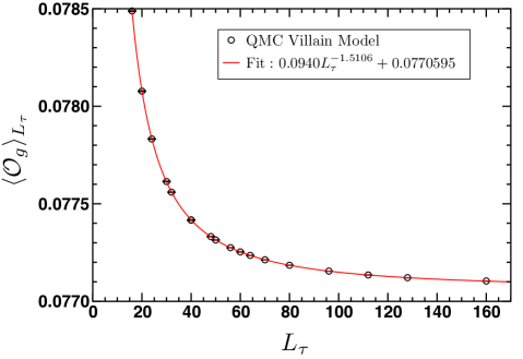
Figure 2: QMC results (open circles) at $K_{c}=0.3330671$ for $\langle\mathcal{O}_{g}\rangle$ in the limit $L\to\infty$ as a function of $L_{\tau}$. The solid red line indicates a fit to the QMC data of the indicated form.

Next we turn to correlations of the “thermal” operator $\mathcal{O}_{g}$. For the Villain model, it is convenient to define this operator by

$$\mathcal{O}_{g}(\tau,{\vec{r}})=\frac{1}{2}{\bf J}^{2}_{(\tau,{\vec{r}})}-\frac{\mu}{U}J^{\tau}_{(\tau,{\vec{r}})}\,.$$ (30)

By suppressing winding number fluctuations in the spatial directions and using system sizes with spatial dimensions $L>L_{\tau}$ Chen et al. (2014) it is possible to effectively calculate $\langle\mathcal{O}_{g}\rangle$ in the limit $L\to\infty$ with finite $L_{\tau}$. Our results are shown in Fig. 2. An extraordinary good agreement with the analytical expression Eq. (16) is evident. The fit shown in Fig. 2 immediately yields

$$\nu=0.6714(10)\,,$$ (31)

in excellent agreement with other recent estimates Campostrini et al. (2001); Burovski et al. (2006); Campostrini et al. (2006) confirming that $\nu$ is slightly larger than $2/3$. In fact, the precision at which $\nu$ can be determined from $\langle\mathcal{O}_{g}\rangle$ makes this a promising venue for a future high precision determination of $\nu$. Furthermore, from Fig. 2 we find that the coefficient $B$ in Eq. (16) is

$$B=0.0940(6).$$ (32)

Recall that the value of $B$ by itself is non-universal, and depends upon the microscopic choices we made in the definition in Eq. (30); however we will combine it below with another observable to obtain a normalization-independent number. For further analysis, it is also useful to note the non-universal value:

$$\langle\mathcal{O}_{g}\rangle_{L_{\tau}\to\infty}=0.0770595(5).$$ (33)

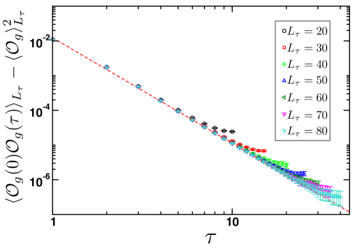
Figure 3: QMC results (open circles) at $K_{c}=0.3330671$ for $\langle\mathcal{O}_{g}(0)\mathcal{O}_{g}(\tau)\rangle_{L_{\tau}}-\langle\mathcal{O}_{g}\rangle^{2}_{L_{\tau}}$ in the limit $L\to\infty$ as a function of the imaginary time, $\tau$. Results are shown for different values of $L_{\tau}$. The dashed red line indicates the $L_{\tau}\to\infty$ limit of $\langle\mathcal{O}_{g}(0)\mathcal{O}_{g}(\tau)\rangle_{L_{\tau}}-\langle\mathcal{O}_{g}\rangle^{2}_{L_{\tau}}\ \to\ 0.0122\tau^{-(6-2/\nu)}$ with $\nu=0.6714$.

Next, we turn to the two-point correlation function of $\mathcal{O}_{g}$. Due to the space-time isotropy of the Villain model, it has the same behavior along the spatial and temporal directions. However, for convenience we focus on the temporal correlations. As before we perform calculations effectively in the $L\to\infty$ limit with a finite $L_{\tau}$. Our results are shown in Fig. 3. The data for individual values of $L_{\tau}$ are first fit to the form $A\left[\tau^{-(6-2/\nu)}+(L_{\tau}-\tau)^{-(6-2/\nu)}\right]+\langle\mathcal{O}_{g}\rangle^{2}_{L_{\tau}}$ for $\tau>6$. This yields values of $A$ that are close to independent of $L_{\tau}$ and we estimate:

$$A=0.0122(15)\,.$$ (34)

The variations in $\nu$ in the fits are small, $\nu=0.671-0.675$, and consistent with the value of $\nu$ obtained above, Eq. (31). Furthermore, the fitted values for $\langle\mathcal{O}_{g}\rangle^{2}_{L_{\tau}}$ are consistent with the actual calculated values of $\langle\mathcal{O}_{g}\rangle_{L_{\tau}}$ and clearly approach $\langle\mathcal{O}_{g}\rangle_{L_{\tau}\to\infty}^{2}$ as determined from Eq. (33).

Finally, we can combine our computations of the one-point and two-point correlators of $\mathcal{O}_{g}$ to obtain a universal number which is independent of the precise definition of $\mathcal{O}_{g}$ and the microscopic details of the action. This is the ratio $\Upsilon$ defined in Eq. (21), and the present Monte Carlo studies yield:

$$\Upsilon=\frac{\sqrt{A}}{B}=1.18(13).$$ (35)

Almost all of the uncertainty in this result arises from the uncertainty in the determination of $A$ which is difficult to calculate with high precision. This result for $\Upsilon$ is in reasonable agreement with the $1/N$ expansion results in Eq. (21), where we have the $N=\infty$ value $\Upsilon=0.97$, and the $1/N$ corrected value at $N=2$ of $\Upsilon=1.41$.

We have also performed simulations directly of Eq. (26) which does not involve the Villain approximation. In this case it is considerably harder to obtain high precision numerical data, however, our preliminary results indicate a value of $\Upsilon$ in very good agreement with the above results for the Villain model.

IV Holography

We have so far obtained systematic results for the conductivity in the high frequency regime $|\omega|\gg T$. We also obtained quantum Monte Carlo results at the discrete Matsubara frequencies $\omega_{n}=2n\pi T$, where $n$ is a non-zero integer. As we noted in Section I, we will now turn to holography to perform the analytic continuation to all Minkowski frequencies.

For the contributions of the energy-momentum tensor terms in Eq. (3), such an analysis has already been carried out in Ref. Witczak-Krempa et al. (2014). So we turn to the extension needed to include the contribution of a scalar operator $\mathcal{O}$.

For the present purposes, the operator $\mathcal{O}$ is any operator in the OPE which obeys the analogs of the Eqs. (16) and (19)

$$\left\langle\mathcal{O}({\bm{x}})\mathcal{O}(0)\right\rangle = \frac{A}{x^{2\Delta}}\quad,\quad T=0;$$

$$\left\langle\mathcal{O}\right\rangle_{T}-\left\langle\mathcal{O}\right\rangle_{T=0} = BT^{\Delta},$$ (36)

which define the normalization independent universal ratio $\Upsilon\equiv\sqrt{A}/B$.

Now take the holographic dual of the same CFT in AdS_D+1 and the corresponding boundary operator $\mathcal{O}({\bm{x}})$ is represented by a bulk scalar field $\varphi({\bm{x}},\tilde{u})$; here $\tilde{u}$ represents the emergent direction, and the AdS_D+1 metric is $L^{2}(d{\bm{x}}^{2}+d\tilde{u}^{2})/\tilde{u}^{2}$ ($L$ is the AdS radius). In the conventional normalization for the bulk scalar, the two-point correlator of $\mathcal{O}$ is Chowdhury et al. (2013)

$$\left\langle\mathcal{O}({\bm{k}})\mathcal{O}(-{\bm{k}})\right\rangle=-(2\Delta-D)\frac{\Gamma(1-\Delta+D/2)}{\Gamma(1+\Delta-D/2)}\left(\frac{k}{2}\right)^{2\Delta-D}$$ (37)

This translates in real space to

$$\left\langle\mathcal{O}({\bm{x}})\mathcal{O}(0)\right\rangle=\frac{\pi^{-D/2}(D-2\Delta)\Gamma(\Delta)\Gamma(1-\Delta+D/2)}{\Gamma(D/2-\Delta)\Gamma(1+\Delta-D/2)}\,\frac{1}{x^{2\Delta}}$$ (38)

For holography to reproduce the $T>0$ expectation values of the CFT with the same universal constant $\Upsilon$, we conclude from Eq. (36) that

$$\left\langle\mathcal{O}\right\rangle_{T}-\left\langle\mathcal{O}\right\rangle_{T=0}=\frac{1}{\Upsilon}\left[\frac{\pi^{-D/2}(D-2\Delta)\Gamma(\Delta)\Gamma(1-\Delta+D/2)}{\Gamma(D/2-\Delta)\Gamma(1+\Delta-D/2)}\right]^{1/2}T^{\Delta}.$$ (39)

Again using the standard AdS/CFT dictionary, we conclude that the bulk scalar must behave as (note that the metric is not modified at $T>0$ near the boundary $\tilde{u}\rightarrow 0$):

$$\varphi({\bm{x}},\tilde{u}\rightarrow 0) = \frac{\tilde{u}^{\Delta}}{(2\Delta-D)}\left(\left\langle\mathcal{O}\right\rangle_{T}-\left\langle\mathcal{O}\right\rangle_{T=0}\right)$$ (40)

$$= \frac{1}{\Upsilon(2\Delta-D)}\left[\frac{\pi^{-D/2}(D-2\Delta)\Gamma(\Delta)\Gamma(1-\Delta+D/2)}{\Gamma(D/2-\Delta)\Gamma(1+\Delta-D/2)}\right]^{1/2}(\tilde{u}\,T)^{\Delta}.$$

The $N=2$ Wilson-Fisher theory has $\Delta=\Delta_{g}$ given by Eq. (5) with $\nu=0.67155(27)$ Campostrini et al. (2001); so $2\Delta-D=3-2/\nu\approx 0.02$ is nearly zero. Fortunately, the coefficient in Eq. (40) has a finite limit ($\approx 0.28/\Upsilon$) as $\Delta\rightarrow D/2$.

We now turn to deducing the consequences of the condensate of $\varphi$ in Eq. (40) at $T>0$. Following the notation of Ref. Witczak-Krempa and Sachdev, 2012, it is convenient to introduce the dimensionless co-ordinate $u$, and the length scale $r_{0}$ by

$$u=\frac{\tilde{u}\,r_{0}}{L^{2}}\quad,\quad r_{0}=\frac{4\pi TL^{2}}{3}.$$ (41)

Then the $T>0$ AdS₄-Schwarzschild metric is

$$ds_{\rm Sch}^{2}=\frac{r_{0}^{2}}{L^{2}u^{2}}\left[-f(u)dt^{2}+dx^{2}+dy^{2}\right]+\frac{L^{2}du^{2}}{u^{2}f(u)}\,,$$ (42)

where

$$f(u)=1-u^{3}\,.$$ (43)

This spacetime is asymptotically ($u\rightarrow 0$) AdS₄, with negative cosmological constant $\propto-1/L^{2}$, and contains a planar black hole with horizon at $u=1$. We simplify notation for the near-boundary behavior of the field $\varphi$ in Eq. (40) by defining

$$\varphi(u\rightarrow 0)=au^{\Delta}+\cdots\,,$$ (44)

where the dots represent terms that decay faster as $u\rightarrow 0$, and $a$ is determined by the definitions above. The field $\varphi$ will couple to the bulk gauge boson, $A_{\mu}$, dual to the current of the CFT like a dilaton, leading to the gauge action

$$\mathcal{S}=\int d^{4}x\sqrt{-g_{\rm Sch}}\left\{-\frac{1}{4g_{4}^{2}}[1+\alpha\varphi(u)]F_{ab}F^{ab}\right\}\,,$$ (45)

where $F_{ab}=\partial_{a}A_{b}-\partial_{b}A_{a}$, $g_{4}$ is the bulk gauge charge, and the coupling $\alpha$ is proportional to the OPE coefficient $\mathcal{C}$ in Eq. (3). As we shall see, the $\omega_{n}\gg T$ asymptotic behavior of the conductivity of the corresponding boundary CFT is

$$\frac{\sigma(i\omega_{n})}{\sigma_{Q}}=\sigma_{\infty}+b_{1}\left(\frac{T}{\omega_{n}}\right)^{\Delta}+\dotsb,$$ (46)

where the dots denote subleading terms. The coefficient $b_{1}$ is as defined in Eq. (4), and it is proportional to the coupling $\alpha$ in Eq. (45). As inputs to the holographic computation we will not use the values of $\alpha$ and $\mathcal{C}$, but directly fit the value of $b_{1}$ to the Monte Carlo results in Eq. (29).

Let us now determine the relation between $b_{1}$ and $a,\alpha$. In the $A_{u}=0$ gauge, the equation of motion which follows from Eq. (45) for the transverse component of the gauge field, $A_{y}$, (choosing $\vec{k}$ along the $x$-direction) is

$$\left((1+\alpha\varphi)fA_{y}^{\prime}\right)^{\prime}-\mathfrak{w}^{2}\frac{(1+\alpha\varphi)}{f}A_{y}=0\,\quad;\quad\mathfrak{w}\equiv\frac{3\omega_{n}}{4\pi T}\,,$$ (47)

where we have defined $(\,)^{\prime}=\partial_{u}(\,)$, and the rescaled imaginary frequency $\mathfrak{w}$. We note that $\mathfrak{w}$ is defined for any value, not only at the discrete Matsubara frequencies. The function $f(u)$ appears in the metric, and was defined in Eq. (43) (the results in this section hold for all $f(u)=1-u^{p}+\cdots$, with $p\geq 1$, so that the boundary metric is AdS₄). To determine the power law $1/\omega_{n}^{\Delta}$ in Eq. (46), we can easily make use of the analysis of Ref. Witczak-Krempa (2014), which relies on the contraction map method employed in Ref. Gulotta et al. (2011). Here, we wish in addition to determine the coefficient $b_{1}$. This can be done perturbatively in $\alpha$, as we now show. It will be advantageous to change the holographic coordinate from $u$ to $z$: $dz/du=1/f(u)$, i.e. $z(u)=\int_{0}^{u}d\bar{u}/(1-\bar{u}^{3})$. Note that for $u\approx 0$, $z$ reduces to $u$. Given the standard AdS/CFT prescription, the solution to Eq. (47) can be parameterized as $A_{y}=e^{-\mathfrak{w}z}+\alpha\tilde{A}$, with $\tilde{A}$ satisfying a Dirichlet condition at $z=0(=u)$. To leading order in $\alpha$, $\tilde{A}$ obeys

$$\partial_{z}^{2}\tilde{A}-\mathfrak{w}^{2}\tilde{A}=\mathfrak{w}e^{-\mathfrak{w}z}\partial_{z}\varphi\,.$$ (48)

This equation can be solved by using a Green’s function,

$$G(z,\bar{z})=-\frac{1}{\mathfrak{w}}\left(\sinh(\mathfrak{w}z)e^{-\mathfrak{w}\bar{z}}~{}\theta(\bar{z}-z)+\bar{z}\leftrightarrow z\right),$$ (49)

where $\partial_{z}^{2}G-\mathfrak{w}^{2}G=\delta(z-\bar{z})$. The current-current correlation function is then given by

$$\langle J_{x}(\mathfrak{w})J_{x}(-\mathfrak{w})\rangle_{T}=\frac{1}{g_{4}^{2}}\partial_{u}A_{y}(u=0)=-\frac{\mathfrak{w}}{g_{4}^{2}}\left(1+\alpha\int_{0}^{\infty}dz~{}e^{-2\mathfrak{w}z}\partial_{z}\varphi+\dotsb\right).$$ (50)

Using the asymptotic behavior for the scalar profile, Eq. (44), we obtain:

$$\frac{\sigma(i\mathfrak{w})}{\sigma_{Q}\sigma_{\infty}} =-\frac{1}{\mathfrak{w}}\partial_{u}A(u=0)$$ (51)

$$=1+\alpha a\frac{\Gamma(\Delta+1)}{2^{\Delta}}\frac{1}{\mathfrak{w}^{\Delta}}+\dotsb,\qquad\text{ for }\mathfrak{w}\gg 1\,.$$ (52)

Comparing to Eq. (46) we find that we can indeed match the finite temperature CFT results, as long as

$$b_{1}=\sigma_{\infty}~{}\alpha\,a\,\frac{\Gamma(\Delta+1)}{2^{\Delta}}\left(\frac{4\pi}{3}\right)^{\Delta}\,.$$ (53)

As a check, we can compare this result with the WKB analysis Witczak-Krempa (2014) done for the asymptotic behavior of $\sigma$ with a holographic model containing the term $\gamma L^{2}C_{abcd}F^{ab}F^{cd}$. For the AdS₄-Schwarzschild metric, this term is also of the form given by Eqs. (44) and (45), with $\alpha\,a=4\gamma$ and $\Delta=3$, which is the scaling dimension of the energy-momentum tensor. Then the result above agrees with the WKB analysis Witczak-Krempa (2014): $b_{1}/\sigma_{\infty}=3\gamma\times(4\pi/3)^{3}$.

We are now ready to use this relation in conjunction with simplest finite-temperature holographic model to determine the charge diffusion constant and the conductivity at zero frequency. Here, it must be kept in mind that we are not including the long-time tails which were discussed in earlier work Witczak-Krempa et al. (2014). The full frequency dependence of the conductivity is discussed in Section IV.2.

IV.1 Holographic model for charge diffusion and conductivity

We shall proceed by examining the simplest holographic ansatz which models a CFT at finite temperature while reproducing its UV behavior. For this we simply assume that the $u\rightarrow 0$ behavior of the scalar profile in Eq. (44) holds all the way up to the horizon at $u=1$. Such an ansatz connects naturally to the previous holographic analyses Myers et al. (2011); Ritz and Ward (2009); Witczak-Krempa and Sachdev (2012) that considered a four-derivative term coupling the Weyl tensor to two field strengths, $\gamma L^{2}C_{abcd}F^{ab}F^{cd}$: for the AdS₄-Schwarzschild metric, this term has a $u^{3}$ dependence for all $u$, both near the boundary $u\rightarrow 0$, and near the horizon $u\rightarrow 1$. We mention that in principle a more detailed holographic analysis can be performed, where one determines the dilaton profile $\varphi(u)$ self-consistently with the metric. It would be interesting to study the resulting IR behavior. We leave this for future investigation, and proceed with our physically motivated ansatz, which, as we shall see, captures many essential features.

The charge diffusion constant for the background in Eq. (45) is well known and is given, for example in Refs. Son and Starinets, 2002; Myers et al., 2011:

$$D=\frac{3}{4\pi T}[1+\alpha\varphi(1)]\int_{0}^{1}du~{}\frac{1}{1+\alpha\varphi(u)}\,.$$ (54)

Working perturbatively in $\alpha$ the above equation for the diffusion constant becomes

$$D\approx\frac{3}{4\pi T}\left[1+\alpha\,a~{}\frac{\Delta}{\Delta+1}\right]=\frac{3}{4\pi T}\left[1+\frac{b_{1}}{\sigma_{\infty}}~{}\frac{\Delta}{\Gamma(\Delta+2)}\left(\frac{3}{2\pi}\right)^{\Delta}\right].$$ (55)

From the last equality, we note that the growth of $b_{1}$ with $\Delta$ must be very rapid in order for an operator with large scaling dimension to make an important contribution to the charge diffusion constant, otherwise that operator will decouple. A similar statement can be made about the d.c. conductivity:

$$\frac{\sigma(0)}{\sigma_{Q}} =\frac{1}{g_{4}^{2}}[1+\alpha\phi(1)]=\frac{1}{g_{4}^{2}}(1+\alpha a)\,,$$ (56)

$$=\sigma_{\infty}+\frac{b_{1}}{\Gamma(\Delta+1)}\left(\frac{3}{2\pi}\right)^{\Delta}\,.$$ (57)

Before discussing the relevance of this analysis to generic CFTs, we point out an important caveat. Namely, that for generic CFTs we expect the conductivity to diverge logarithmically in the small frequency limit $\omega/T\rightarrow 0$ due to long-time tails. This classical effect leads to the slow decay of correlators of conserved currents at long times; see the discussion in Refs. Witczak-Krempa and Sachdev (2012); Witczak-Krempa et al. (2014) for further details. Such long-time tails do not occur in the tree-level (or classical) holographic models that we consider due to an implicit limit of infinite number of CFT fields. Our holographic analysis therefore cannot describe the conductivity of the O(2) CFT when $\omega\ll T$. (We point out that holography can capture long-time tails if $1/N$ quantum corrections are taken into account Caron-Huot and Saremi (2010).) To circumvent the need to refer to long-time tails, one could replace the statements about $\omega=0$, such as Eq. (57), by equivalent statements at small but finite frequencies, say on the order of the temperature. The analysis above becomes more involved but we expect similar conclusions for the holographic model under consideration.

In a typical CFT once temperature is turned on there will be an infinite number of operators which will obtain expectation values proportional to the temperature to the appropriate power. The large-frequency behavior of various correlators is thus expected to receive contributions from an infinite number of such operators, which appear in the corresponding OPE. In other words, we expect generically that the true holographic background should contain additional fields with profiles that are needed to reproduce higher order terms in the OPE at large Euclidean frequencies. Naively, one would expect that for real frequencies far below the temperature, all such operators should become important in determining low energy quantities such as charge diffusion (where the OPE badly diverges). However, the holographic model suggests that high scaling dimension operators decouple rapidly if their OPE coefficient does not grow factorially. In that case, the diffusion constant and d.c. conductivity can be well described with only the lowest dimension operators. If, on the other hand, the OPE coefficients grow rapidly, compensating for the suppression factors found above, the holographic background can deviate considerably from the naive AdS₄-Schwarzschild form. In fact, higher spin fields in the bulk (corresponding to higher spin CFT operators) can become important, spoiling the simple background-metric description. In such a situation, one would question not only the photon equation of motion Eq. (45) but also the boundary conditions used for the bulk modes at $u=1$. Thus, a natural conjecture is that it is precisely for theories where the OPE coefficients do not grow considerably that finite temperature can be modeled with a horizon. In those theories, the leading correction to the low frequency conductivity should come from the lowest dimension operator, as we have considered.

IV.2 Comparing holography with quantum Monte Carlo

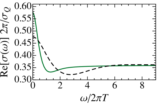
Figure 4: a) Holographic fit (line) to Quantum Monte Carlo data for the conductivity of a model in its O$(2)$ quantum critical regime (dots). The holographic parameters are: $\Delta=3/2,a\alpha=0.6$. b) The corresponding conductivity on the real (Minkowski) frequency axis (solid line). The dashed line corresponds to the holographic fit obtained in Ref. Witczak-Krempa et al. (2014), where an ad hoc rescaling of temperature was needed.

We now solve the equation of motion for $A_{y}$, Eq. (47), in order to study the full frequency dependence of the conductivity, especially for real frequencies. We solve the differential equation numerically with in-falling boundary conditions at the horizon Myers et al. (2011). The solution can be obtained in the full complex plane of frequency. In particular, we can compare the holographic result with QMC data Witczak-Krempa et al. (2014) for the O$(2)$ quantum critical theory, which is obtained for imaginary frequencies $\omega_{n}\geq 2\pi T$, as shown in Fig. 4. Most notably, we observe in Fig. 4 that the holographic result fits the QMC data without the need of a temperature rescaling. A rescaling was needed previously Witczak-Krempa et al. (2014); Chen et al. (2014) because the holographic theory used then had the scaling dimension fixed to $\Delta=3$, i.e. the dimension of the energy-momentum tensor. In contrast, when the dimension is chosen to be that of the thermal operator $\Delta=\Delta_{g}=3-1/\nu\approx 1.5$, as expected from the OPE analysis above, a good fit results without the need for an ad hoc rescaling. This fitting effectively determines the values of $b_{1}$ and $a\alpha$. We can now use these values to determine the conductivity along the Minkowski frequency axis, and this leads to our main result in Fig. 4.

We emphasize that certain qualitative features obtained using the previous holographic approach (which required rescaling) remain unchanged with our new result, namely:

• particle-like conductivity,

• similar pole structure, i.e. quasinormal spectrum (shown in Fig. 5),

• validity of sum rules Gulotta et al. (2011); Witczak-Krempa and Sachdev (2012); see Section VI.

The first two statements are related because a particle-like conductivity follows from the presence of a pole on the negative imaginary-frequency axis, as shown in Fig. 5. We note that such a purely damped pole for $\sigma(\omega/T)$ was found in the O($N$) CFT at large-$N$ by including $1/N$ effects Witczak-Krempa et al. (2012); Witczak-Krempa and Sachdev (2012). In contrast, a vortex-like response would have a zero on the imaginary axis; see Fig. 7 for two explicit examples. This purely damped pole dictates the “topology” of the full pole/zero spectrum as the poles and zeros appear in an alternating fashion. Mathematically, it follows because the sign of the scalar coupling $\alpha$ dictates the presence of a particle-like ($\alpha>0$) or vortex-like ($\alpha<0$) conductivity for any allowed $\Delta$.

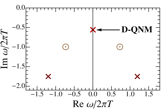
Figure 5: The location of the small-frequency poles (crosses) and zeros (circles) of the holographic conductivity $\sigma(\omega)$ in the complex frequency plane. The parameters used are the same as those use to fit the O(2) QCP, see Fig. 4. The dominant, purely damped pole is denoted by D-QNM, where QNM stands for quasinormal mode.

V Fermionic CFTs

We briefly discuss extension to CFTs with Dirac fermions. A large class of such CFTs differ crucially from the O($N$) CFT by the absence of any scalar operator $\mathcal{O}$ in the $JJ$ OPE with scaling dimension $\Delta<3$. Consequently, the leading term in the large $\omega$ dependence of the conductivity in Eqs. 3 and (4) is just given by that from the OPE with the energy-momentum tensor. And such terms were implicitly accounted for in the previous holographic studies Myers et al. (2011); Witczak-Krempa et al. (2014).

The basic point is already evident from the CFT of free (two-component) Dirac fermions. The Lagrangian is

$$\mathcal{L}=\bar{\psi}i\gamma_{\mu}\partial_{\mu}\psi\,,$$ (58)

where $\gamma_{\nu}$ are the Euclidean gamma matrices $\gamma_{\nu}^{\dagger}=\gamma_{\nu}$ satisfying the Clifford algebra $\{\gamma_{\mu},\gamma_{\nu}\}=2\delta_{\mu\nu}$. The conserved U(1) current is $J_{\mu}=\bar{\psi}\gamma_{\mu}\psi$. The integral expression for the finite-$T$ conductivity can be simply obtained:

$$\frac{\sigma(i\omega_{n})}{\sigma_{Q}}=\frac{1}{\omega_{n}}T\sum_{\nu_{n}}\int\frac{d^{2}\vec{k}}{(2\pi)^{2}}\frac{1}{\epsilon_{k}^{2}+\nu_{n}^{2}}\left[\frac{4k_{x}^{2}+\omega_{n}^{2}}{\epsilon_{k}^{2}+(\nu_{n}+\omega_{n})^{2}}-\frac{4k_{x}^{2}}{\epsilon_{k}^{2}+\nu_{n}^{2}}\right]\,,$$ (59)

where $\nu_{n}=\pi T(2n+1)$ and $\epsilon_{k}=k$. This leads to the following high frequency behavior $\omega_{n}\gg T$:

$$\frac{\sigma(i\omega_{n})}{\sigma_{Q}} =\frac{1}{16}-\frac{T}{2\pi\omega_{n}}\sum_{m=1}\left(\frac{-T^{2}}{\omega_{n}^{2}}\right)^{m}s_{m}$$ (60)

$$=\frac{1}{16}+\frac{3\zeta(3)T^{3}}{\pi\omega_{n}^{3}}-\frac{180\zeta(5)T^{5}}{\pi\omega_{n}^{5}}+\mathcal{O}((T/\omega_{n})^{7})\,,$$ (61)

where $s_{m}=(2^{2m}-1)(2m)!\,\zeta(2m+1)$, and $\zeta$ is the Riemann zeta function. We refer the reader to Appendix E for further details on the calculation.

The most notable feature of Eq. (61) is the absence of the $(T/\omega_{n})^{2}$ term (found in Eq. (109) for the $N=\infty$ O($N$) model), and the presence of a leading $(T/\omega_{n})^{3}$ term. The latter corresponds to the term associated with the energy-momentum tensor in Eq. (3), and we show in Appendix E that the coefficient of $(T/\omega_{n})^{3}$ in Eq. (61) is consistent with the value of the OPE coefficient $\mathcal{C}_{T}$. Such a $(T/\omega_{n})^{3}$ term is clearly generic to all CFTs.

The absence of a scalar operator with $\Delta<3$ is also easily understood. A likely candidate for a scalar is $\bar{\psi}\psi$, but such a mass term for Dirac fermions breaks both time-reversal and parity symmetries in 2+1 dimensions; this is the case even if such a mass term acquires an expectation value only at finite temperature. It is now also clear that such a scalar is also absent in interacting CFTs in which the Dirac fermions are coupled to gauge fields (such as QED3), at least in the context of the $1/N_{f}$ expansion Wen and Wu (1993); Kaul and Sachdev (2008); Klebanov et al. (2012), where $N_{f}$ is the number of flavors of Dirac fermions. If the CFT has both Dirac fermions and elementary scalar fields $\phi_{\alpha}$ (as in the Gross-Neveu model), then in general an operator $\mathcal{O}\sim\phi_{\alpha}^{2}$ with $\Delta<3$ will be generated at $T>0$ unless this is protected by additional symmetries, such as supersymmetry.

VI Sum rules

The asymptotic behavior of the conductivity derived from the current-current OPE can be used to establish the finite-$T$ conductivity sum rules recently put forward Gulotta et al. (2011); Witczak-Krempa and Sachdev (2012); Witczak-Krempa (2014):

$$\int_{0}^{\infty}d\omega[\operatorname{Re}\sigma(\omega/T)-\sigma(\infty)] =0\,,\,$$ (62)

$$\int_{0}^{\infty}d\omega\left[\operatorname{Re}\left\{\frac{1}{\sigma(\omega/T)}\right\}-\frac{1}{\sigma(\infty)}\right] =0\,.$$ (63)

The second sum rule Witczak-Krempa and Sachdev (2012) is the S-dual or particle-vortex dual of the first one. An essential ingredient for the sum rules to be valid is that the integrand must be integrable. Assuming this holds, one can extend the integration to be from $-\infty$ to $+\infty$, since in both cases the argument is even. Eq. (62) can then be proven by performing a contour integration in the upper complex half-plane, where $\sigma(z)$ is analytic by virtue of the retardedness of the current two-point function. A similar argument holds for Eq. (63), as we explain in Section VI.3.

Our main objective is thus to show that the integrand decays sufficiently fast as $\omega/T\rightarrow\infty$. This is precisely the regime where our OPE analysis applies. As we discussed above, see Eq. (3), the operator with the smallest scaling dimension and finite thermal expectation value appearing in the current-current OPE dictates how fast $\operatorname{Re}\sigma(\omega/T)-\sigma(\infty)$ vanishes. Along the imaginary axis, the decay is $(T/\omega_{n})^{\Delta}$, where $\Delta$ is the dimension of the operator in question. Non-scalar operators, i.e. with a finite spin $\ell>0$, such as the energy-momentum tensor ($\ell=2$) cannot cause any problems at large frequencies because their scaling dimension is guaranteed to be sufficiently large, being bounded from below by unitarity: $\Delta_{\ell>0}\geq\ell+1$, for CFTs in 2+1D. For instance, the energy-momentum tensor saturates the $\ell=2$ bound yielding a $(T/\omega_{n})^{3}$ contribution to the conductivity on the imaginary axis. This term does not even contribute to $\operatorname{Re}\sigma$ at real frequencies, which is of interest for the sum rule. In contrast, scalar operators ($\ell=0$) have the potential of making the integrand of Eq. (62) non-integrable because of the weaker lower bound, $\Delta_{\ell=0}\geq(D-2)/2=1/2$. However, in all the CFTs known to the authors, the scalars appearing the $JJ$ OPE have sufficiently high scaling dimension to ensure that the sum rule Eq. (62) is well-defined. As it is difficult to make rigorous statements in general, we focus on the two families of CFTs discussed above.

VI.1 O$(N)$ model

For the O($N$) vector model, the leading operator in the $JJ$ OPE is the thermal operator $\mathcal{O}_{g}$ discussed above. It has scaling dimension $\Delta_{g}=3-1/\nu$. We thus need $\Delta_{g}>1$, i.e. $\nu>1/2$, for the sum rule to be well-defined. Now, for $N=2$, it is known from Monte Carlo that $\nu$ is slightly greater than $2/3$. Also, there is strong numerical and analytical evidence that $\nu$ increases with $N$, until it reaches the exact value $\nu=1$ at $N=\infty$. We thus conclude that the conductivity of the O$(N)$ CFT decays sufficiently fast for the sum rule to hold for all $N>1$. When $N=\infty$, the decay is $(T/\omega)^{2}$ on the real axis, since $\Delta_{g}\big{|}_{N=\infty}=2$. In that case, the sum rule, Eq. (62), was previously shown to hold by two of us Witczak-Krempa and Sachdev (2012).

VI.2 Fermionic CFTs

For the free Dirac CFT, we have shown that the leading operator that appears in the $JJ$ OPE is the energy-momentum tensor, which has dimension $\Delta=3$, ruling out potentially dangerous scalars. An explicit analysis Witczak-Krempa and Sachdev (2012) has indeed shown that the sum rule holds. This is also the case for interacting CFTs in which $N_{f}$ Dirac fermions are coupled to gauge fields (at least in the context of the $1/N_{f}$ expansion). These theories are thus expected to satisfy the sum rule Eq. (62).

VI.3 Dual sum rule

The dual sum rule, Eq. (63), follows from the sum rule for $\sigma$ Eq. (62) for two reasons: 1) the large-frequency asymptotics of $1/\sigma$ are the same as those of $\sigma$ on the imaginary axis; 2) $\sigma(z)$ has no zeros in the upper half-plane. The first point can be easily seen by inverting $\sigma(i\omega_{n})=\sigma_{\infty}+b_{1}(T/\omega_{n})^{\Delta}+\cdots$, and keeping the leading high-frequency term. It thus shows that if $\operatorname{Re}\sigma(\omega/T)-\sigma(\infty)$ is integrable as $\omega/T\rightarrow\infty$, then $\operatorname{Re}[1/\sigma(\omega/T)]-[1/\sigma(\infty)]$ also is. The second point follows from the analyticity of $\sigma(z)$ in the upper half-plane. It can be seen using the spectral representation of the current-current correlator.

In Appendix F, we explicitly verify that the dual sum rule Eq. (63) is respected by both the O$(N)$ model in the $N=\infty$ limit, and by the Dirac CFT. These constitute the first non-holographic checks.

VII Conclusions

Our paper has used the operator product expansion to obtain insight into the frequency dependence of the quantum-critical conductivity near the superfluid-insulator transition in 2 spatial dimensions at non-zero temperatures; more generally, our results apply to conformal field theories in 2+1 dimensions.

At frequencies $\omega\gg T$, we found that the conductivity had contributions $\sim(T/\omega)^{\Delta}$, where $\Delta$ is the scaling dimension of any operator appearing in the OPE of two currents that acquires a non-zero expectation value at $T>0$. For the CFT describing the superfluid-insulator transition, the smallest such $\Delta$ is that associated with the “thermal” operator $\phi_{\alpha}^{2}$ (where $\phi_{1}+i\phi_{2}$ is the complex superfluid order parameter), and this has scaling dimension $\Delta_{g}=3-1/\nu$, where $\nu$ is the correlation length exponent. The next allowed operator is the energy-momentum tensor, which has $\Delta=3$. The contribution of the energy-momentum tensor is the leading term for CFTs which don’t have allowed “thermal” operators, which includes wide classes of CFTs with Dirac fermions.

We computed the OPEs (and associated frequency dependence of the conductivity) of the $\phi_{\alpha}^{2}$ operator, and of the energy-momentum tensor, for the O($N$) CFT using the vector $1/N$ expansion. These results, and prior computations for the O($N$) CFT, were found to be in excellent agreement with quantum Monte Carlo simulations.

We then addressed the question of extending these $\omega\gg T$ results to smaller $\omega$. For all non-zero, Euclidean Matsubara frequencies, the low frequency conductivity can be obtained in a controlled manner using the vector $1/N$ expansion. However, this expansion fails for small real Minkowski frequencies Damle and Sachdev (1997), and physically motivated resummations are required. For quantum systems with quasiparticle excitations, the low frequency behavior is conventionally obtained by the Boltzmann equation. For strongly interacting CFTs without quasiparticles, we have advocated Witczak-Krempa et al. (2014) holographic methods. Here, we used the large $\omega$ behavior obtained from the OPE to determine the structure of the holographic theory, and then solved the classical holographic theory to obtain the desired small $\omega$ dependence of the conductivity. In this holographic mapping, we truncated the OPE to the leading “thermal” operator, and presented evidence that the contributions of high dimension operators can be suppressed even at low frequencies.

Finally, we noted how conductivity the sum rules in Eqs. (62,63) can be established from information on the operator product expansion.

Appendix A Correlators of the energy-momentum tensor

Ref. Chowdhury et al. (2013) obtained a number of results for the 3-point correlator between the energy-momentum tensor and the conserved O($N$) current. This appendix will translate those results into the form required for the OPE in Eq. (3).

A.1 O$(N)$ model

First, we consider the correlators of the O($N$) theory in Eq. (6) at its critical point for $N=\infty$. The 2-point correlator of the energy-momentum tensor is

$$\frac{1}{N}\left\langle T_{\mu\nu}({\bm{k}})T_{\rho\sigma}(-{\bm{k}})\right\rangle = \frac{k^{3}}{512}\left(\delta_{\mu\rho}\delta_{\nu\sigma}+\delta_{\nu\rho}\delta_{\mu\sigma}-\delta_{\mu\nu}\delta_{\rho\sigma}+\delta_{\mu\nu}\frac{k_{\rho}k_{\sigma}}{k^{2}}+\delta_{\rho\sigma}\frac{k_{\mu}k_{\nu}}{k^{2}}\right.$$ (64)

$$\left.-\delta_{\mu\rho}\frac{k_{\nu}k_{\sigma}}{k^{2}}-\delta_{\nu\rho}\frac{k_{\mu}k_{\sigma}}{k^{2}}-\delta_{\mu\sigma}\frac{k_{\nu}k_{\rho}}{k^{2}}-\delta_{\nu\sigma}\frac{k_{\mu}k_{\rho}}{k^{2}}+\frac{k_{\mu}k_{\nu}k_{\rho}k_{\sigma}}{k^{4}}\right).$$

For the 3-point $TJJ$ correlator, from the results of Ref. Chowdhury et al. (2013) we obtain

$$\lim_{|\omega|\gg p}\left\langle J_{x}({\bm{\omega}})J_{x}(-{\bm{\omega}}+{\bm{p}})T_{\mu\nu}(-{\bm{p}})\right\rangle=\mbox{contact terms}+\frac{O_{\mu\nu}({\bm{p}})}{\omega^{2}}+\dotsb,$$ (65)

where ${\bm{\omega}}=(\omega,0,0)$. Some non-zero values of $O_{\mu\nu}$ are

$$O_{\tau\tau} =0\,, O_{xx} =|\omega_{1}|^{3}/64\,, O_{yy} =-|\omega_{1}|^{3}/64\,, {\bm{p}}=(\omega_{1},0,0);$$ for

$$O_{\tau\tau} =0\,, O_{xx} =0\,, O_{yy} =0\,, {\bm{p}}=(0,p_{x},0);$$ for

$$O_{\tau\tau} =-|p_{y}|^{3}/64\,, O_{xx} =|p_{y}|^{3}/64\,, O_{yy} =0\,, {\bm{p}}=(0,0,p_{y});$$ for

$$O_{\tau x} =-|p|^{3}/(64\sqrt{2})\,, {\bm{p}}=(p,p,0);\;\,$$ for (66)

To convert this information into an OPE, we need the two-point correlation matrix of the diagonal components of $T_{\mu\nu}$ which we define as $C_{\{\mu\nu\}}({\bm{p}})=\left\langle T_{\mu\mu}({\bm{p}})T_{\nu\nu}(-{\bm{p}})\right\rangle$. From Eq. (64) we obtain

$$C_{\{\mu\nu\}}({\bm{p}})=\frac{N|p|^{3}}{512}\left(\begin{array}[]{ccc}0&0&0\\ 0&1&-1\\ 0&-1&1\end{array}\right)\quad,\quad\mbox{for ${\bm{p}}=(p,0,0)$},$$ (67)

and similarly for other orientations.

Now we assume the OPE

$$\lim_{|\omega|\gg p}J_{x}({\bm{\omega}})J_{x}(-{\bm{\omega}}-{\bm{p}})=\sum_{\mu}B_{\mu}\frac{T_{\mu\mu}({\bm{p}})}{\omega^{2}}+\dotsb$$ (68)

Then from Eqs. (66,67,68) we have the constraints

$$\frac{N}{512}(B_{x}-B_{y}) = \frac{1}{64}$$

$$\frac{N}{512}(B_{\tau}-B_{y}) = 0$$

$$\frac{N}{512}(B_{\tau}-B_{x}) = -\frac{1}{64}\,.$$ (69)

From the last constraint in Eq. (66) we have

$$\frac{N}{512\sqrt{2}}\left(-B_{x}-B_{\tau}+2B_{y}\right)=-\frac{1}{64\sqrt{2}}\,.$$ (70)

So a consistent solution (up to the vanishing trace) is

$$B_{\tau}=0\quad,\quad B_{x}=\frac{8}{N}\quad,\quad B_{y}=0\,.$$ (71)

So we have our main result for the OPE of the O($N$) model

$$\lim_{|\omega|\gg p}J_{x}({\bm{\omega}})J_{x}(-{\bm{\omega}}-{\bm{p}})=\frac{8}{N}\frac{T_{xx}({\bm{p}})}{\omega^{2}}+\dotsb.$$ (72)

From Eq. (3), and using $\gamma=-1/12$ Chowdhury et al. (2013), this leads to the value of $\mathcal{C}_{T}$ in Eq. (10).

A.2 Fermions

Next, we consider a theory of 2-component Dirac fermions with $N_{f}$ flavors, each with the Lagrangian in Eq. (58). The 2-point correlator of the energy-momentum tensor has the same form as Eq. (64)

$$\frac{1}{N_{f}}\left\langle T_{\mu\nu}({\bm{k}})T_{\rho\sigma}(-{\bm{k}})\right\rangle = \frac{k^{3}}{256}\left(\delta_{\mu\rho}\delta_{\nu\sigma}+\delta_{\nu\rho}\delta_{\mu\sigma}-\delta_{\mu\nu}\delta_{\rho\sigma}+\delta_{\mu\nu}\frac{k_{\rho}k_{\sigma}}{k^{2}}+\delta_{\rho\sigma}\frac{k_{\mu}k_{\nu}}{k^{2}}\right.$$ (73)

$$\left.-\delta_{\mu\rho}\frac{k_{\nu}k_{\sigma}}{k^{2}}-\delta_{\nu\rho}\frac{k_{\mu}k_{\sigma}}{k^{2}}-\delta_{\mu\sigma}\frac{k_{\nu}k_{\rho}}{k^{2}}-\delta_{\nu\sigma}\frac{k_{\mu}k_{\rho}}{k^{2}}+\frac{k_{\mu}k_{\nu}k_{\rho}k_{\sigma}}{k^{4}}\right)\,.$$

For the 3-point $TJJ$ correlator, the results of Ref. Chowdhury et al. (2013) take the form in Eq. (65) with the following values of $O_{\mu\nu}$

$$O_{\tau\tau} =0\,, O_{xx} =|\omega_{1}|^{3}/64\,, O_{yy} =-|\omega_{1}|^{3}/64\,, {\bm{p}}=(\omega_{1},0,0);$$ for

$$O_{\tau\tau} =|p_{x}|^{3}/64\,, O_{xx} =0\,, O_{yy} =-|p_{x}|^{3}/64\,, {\bm{p}}=(0,p_{x},0);$$ for

$$O_{\tau\tau} =0\,, O_{xx} =0\,, O_{yy} =0\,, {\bm{p}}=(0,0,p_{y});$$ for

$$O_{\tau x} =-|p|^{3}/(32\sqrt{2})\,, {\bm{p}}=(p,p,0)\,.\;$$ for (74)

Now the constraints are

$$\frac{N_{f}}{256}(B_{x}-B_{y}) = \frac{1}{64}$$

$$\frac{N_{f}}{256}(B_{\tau}-B_{y}) = \frac{1}{64}$$

$$\frac{N_{f}}{256}(B_{\tau}-B_{x}) = 0\,.$$ (75)

From the last constraint in Eq. (74) we have

$$\frac{N_{f}}{256\sqrt{2}}\left(-B_{x}-B_{\tau}+2B_{y}\right)=-\frac{1}{32\sqrt{2}}$$ (76)

So a consistent solution (up to the trace) is

$$B_{\tau}=0\quad,\quad B_{x}=0\quad,\quad B_{y}=-\frac{4}{N_{f}}$$ (77)

Then we have the main result for the OPE of the fermion theory

$$\lim_{|\omega|\gg p}J_{x}({\bm{\omega}})J_{x}(-{\bm{\omega}}-{\bm{p}})=-\frac{4}{N_{f}}\frac{T_{yy}({\bm{p}})}{\omega^{2}}+\dotsb.$$ (78)

From Eq. (3), and using $\gamma=1/12$ Chowdhury et al. (2013), this leads to

$$\mathcal{C}_{T}=\frac{2}{N_{f}}\,.$$ (79)

A.3 Holography

Using a holographic theory with Einstein-Maxwell terms along with a coupling $\gamma$ to the Weyl tensor, the results of Ref. Chowdhury et al. (2013) translate to the following correlators (up to an overall normalization dependent upon Newton’s constant)

$$\lim_{|\omega|\gg p}\left\langle J_{x}({\bm{\omega}})J_{x}(-{\bm{\omega}}-{\bm{p}})\Bigl{(}T_{xx}({\bm{p}})-T_{yy}({\bm{p}})\Bigr{)}\right\rangle = \frac{|p|^{3/2}}{4\omega^{2}}\quad,\quad{\bm{p}}=(p,0,0)$$

$$\lim_{|\omega|\gg p}\left\langle J_{x}({\bm{\omega}})J_{x}(-{\bm{\omega}}-{\bm{p}})\Bigl{(}T_{yy}({\bm{p}})-T_{\tau\tau}({\bm{p}})\Bigr{)}\right\rangle = -\frac{(1+12\gamma)|p|^{3/2}}{8\omega^{2}}\quad,\quad{\bm{p}}=(0,p,0)$$

$$\lim_{|\omega|\gg p}\left\langle J_{x}({\bm{\omega}})J_{x}(-{\bm{\omega}}-{\bm{p}})\Bigl{(}T_{xx}({\bm{p}})-T_{\tau\tau}({\bm{p}})\Bigr{)}\right\rangle = \frac{(1-12\gamma)|p|^{3/2}}{8\omega^{2}}\quad,\quad{\bm{p}}=(0,0,p)$$ (80)

We note that the above results are entirely consistent with the O($N$) model ($N\rightarrow\infty$) results for $\gamma=-1/12$, and with the free fermion results for $\gamma=1/12$, just as expected. For a general CFT, proceeding as in the previous subsections, we obtain Eq. (3).

Appendix B Correlators of the O($N$) model at $T=0$

B.1 Two-point function of $\mathcal{O}_{g}$

The $T=0$ correlators of $Z$ in Eq. (11) have been evaluated at some length in Ref. Podolsky and Sachdev (2012), including the two-point correlator of $\mathcal{O}_{g}$. We recall here the needed results.

The computation proceeds by expanding about the large $N$ saddle point of Eq. (11) after setting $v=\infty$. We denote the saddle point value of $i\widetilde{\lambda}$ as $\sqrt{N}r$, and the fluctuation about the saddle point as $i\lambda$:

$$\widetilde{\lambda}=-i\sqrt{N}r+\lambda.$$ (81)

The equation determining the value of $r$ is

$$\frac{1}{g}=\int_{\bm{p}}\frac{1}{p^{2}+r}.$$ (82)

The quantum critical point has $r=0$ at $T=0$, and so it is $g=g_{c}$ where

$$\frac{1}{g_{c}}=\int_{\bm{p}}\frac{1}{p^{2}}.$$ (83)

A standard $1/N$ expansion then yields the 2-point correlator of $\lambda$ as Podolsky and Sachdev (2012)

$$G_{\lambda\lambda}(p) = 16p-\frac{512}{N}\int_{\bm{k}}\frac{1}{k|{\bm{k}}-{\bm{p}}|}+\frac{256p}{N}\int_{\bm{k}}\frac{1}{({\bm{p}}\cdot{\bm{k}})}\left[\frac{1}{|{\bm{k}}-{\bm{p}}|}-\frac{1}{|{\bm{k}}+{\bm{p}}|}\right]+\frac{512}{N}\int_{\bm{k}}\frac{({\bm{p}}\cdot{\bm{k}})}{pk^{2}|{\bm{p}}-{\bm{k}}|}$$ (84)

$$= 16p-\frac{128}{N\pi^{2}}\left(2\Lambda-p\right)+\frac{256p}{N\pi^{2}}\ln\left(\frac{\Lambda}{p}\right)+\frac{256p}{3N\pi^{2}}\left(\ln\left(\frac{\Lambda}{p}\right)+\frac{1}{3}\right)$$

$$= -\frac{256\Lambda}{N\pi^{2}}+16p\left[1+\frac{64}{3\pi^{2}N}\left(\ln\left(\frac{\Lambda}{p}\right)+\frac{11}{24}\right)\right];$$

the last line above corrects a typographical error in the last line of Eq. (B14) of Ref. Podolsky and Sachdev (2012). Here $\Lambda$ is a relativistic hard-momentum cutoff. The scaling dimension of $\lambda$ is the same as that of $\phi_{\alpha}^{2}$, which is $3-1/\nu$, and so using Eqs. (14,13) we verify that we have at order $1/N$

$$G_{\lambda\lambda}(p)\sim\mbox{constant}+\frac{16}{C_{\lambda}^{2}}\,p^{3-2/\nu},$$ (85)

with the exponent $\nu$ given by

$$\nu=1-\frac{32}{3\pi^{2}N}+\mathcal{O}(1/N^{2}),$$ (86)

and

$$C_{\lambda}=\Lambda^{1-1/\nu}\left(1-\frac{44}{9\pi^{2}N}+\mathcal{O}(1/N^{2})\right).$$ (87)

B.2 Three-point function

To determine the OPE coefficient $\mathcal{C}_{g}$ in Eq. (3) we compute the associated 3-point correlator, as in Eq. (65). At leading order in $1/N$, this is given by the Feynman graph in Fig. 6, and leads to

$$\left\langle J_{x}({\bm{\omega}})J_{x}(-{\bm{\omega}}+{\bm{p}})\mathcal{O}_{g}(-{\bm{p}})\right\rangle = \frac{32p}{\sqrt{N}}\int\frac{d^{2}\vec{k}}{4\pi^{2}}\int_{-\infty}^{\infty}\frac{d\epsilon}{2\pi}\frac{4k_{x}^{2}}{(\epsilon^{2}+k^{2})^{2}((\epsilon+\omega)^{2}+k^{2})}$$ (88)

$$= \frac{4p}{\sqrt{N}|\omega|}\,,$$

where we have retained only the leading term in the $p\rightarrow 0$ limit.

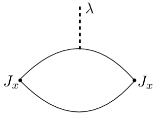
Figure 6: Feynman graph for the computation of $\mathcal{C}_{g}$, Eq. (88). The full line is the $\phi_{\alpha}$ propagator, and the dashed line is the $\lambda$ propagator.

Using Eq. (14), we then obtain Eq. (15).

Appendix C Correlators of the O($N$) model at $T>0$

An extensive study of the $T>0$ correlators of the O($N$) CFT was provided in Ref. Chubukov et al. (1994) using the $1/N$ expansion. Here we present the extensions needed for our purposes.

The first step in the $1/N$ expansion is the determination of the saddle-point value of $i\widetilde{\lambda}$. Solving the extension of Eq. (82) at $T>0$ and $g=g_{c}$ now yields Chubukov et al. (1994)

$$r=\Theta^{2}T^{2}\,,$$ (89)

where $\Theta$ is given in Eq. (18).

For the computation of $\left\langle\mathcal{O}_{g}\right\rangle_{T}$ at $T>0$, we need the following polarization functions, defined in Ref. Chubukov et al. (1994), which determine the propagator of $\lambda$:

$$\Pi(q,\epsilon_{n}) = T\sum_{\omega_{n}}\int\frac{d^{2}\vec{k}}{4\pi^{2}}\frac{1}{(k^{2}+\omega_{n}^{2}+\Theta^{2}T^{2})((\vec{k}+\vec{q})^{2}+(\epsilon_{n}+\omega_{n})^{2}+\Theta^{2}T^{2})}$$

$$= \frac{1}{8(q^{2}+\epsilon_{n}^{2})^{1/2}}+\frac{(2\epsilon_{n}^{2}-q^{2})\Theta^{3}T^{3}}{(q^{2}+\epsilon_{n}^{2})^{3}}\frac{(1-6\Xi)}{3\pi}+\mathcal{O}\left(\frac{T^{5}}{(q,\epsilon_{n})^{6}}\right)$$

$$\Pi(0,0) = \frac{\sqrt{5}}{8\pi\Theta T}$$

$$\Pi_{2}(q,\epsilon_{n}) = T\sum_{\omega_{n}}\int\frac{d^{2}\vec{k}}{4\pi^{2}}\frac{1}{(k^{2}+\omega_{n}^{2}+\Theta^{2}T^{2})^{2}((\vec{k}+\vec{q})^{2}+(\epsilon_{n}+\omega_{n})^{2}+\Theta^{2}T^{2})}$$ (90)

$$= \Pi(0,0)\frac{(q^{2}+\epsilon_{n}^{2})}{(q^{2}+\epsilon_{n}^{2})^{2}+4\Theta^{2}T^{2}\epsilon_{n}^{2}}+\mathcal{O}\left(\frac{T^{3}}{(q,\epsilon_{n})^{6}}\right)$$

where

$$\Xi=\frac{1}{\Theta^{3}}\int_{\Theta}^{\infty}dx\frac{x^{2}}{e^{x}-1}.$$ (91)

From these ingredients, a perturbative expansion from the $T>0$ version of the action in Eq. (11) yields Chubukov et al. (1994); Podolsky and Sachdev (2012)

$$\left\langle\mathcal{O}_{g}\right\rangle_{T}=C_{\lambda}\sqrt{N}\left[\Theta^{2}T^{2}-\frac{2}{N}\frac{1}{\Pi(0,0)}\int\frac{d^{2}q}{4\pi^{2}}T\sum_{\epsilon_{n}}\frac{\Pi_{2}(q,\epsilon_{n})}{\Pi(q,\epsilon_{n})}+\mathcal{O}(1/N^{2})\right]$$ (92)

From Eq. (90) we can extract out the portion of integral which has a quadratic ultraviolet divergence

$$\frac{1}{\Pi(0,0)}\int\frac{d^{2}\vec{q}}{4\pi^{2}}T\sum_{\epsilon_{n}}\frac{\Pi_{2}(q,\epsilon_{n})}{\Pi(q,\epsilon_{n})} = \int\frac{d^{2}\vec{q}}{4\pi^{2}}T\sum_{\epsilon_{n}}\left[\frac{\Pi_{2}(q,\epsilon_{n})}{\Pi(0,0)\Pi(q,\epsilon_{n})}-\frac{8}{(q^{2}+\epsilon_{n}^{2})^{1/2}}\right]$$ (93)

$$~{}~{}~{}~{}~{}~{}+\int\frac{d^{2}\vec{q}}{4\pi^{2}}T\sum_{\epsilon_{n}}\frac{8}{(q^{2}+\epsilon_{n}^{2})^{1/2}}$$

Examination of the subleading terms from Eq. (90) now shows that the first integral in Eq. (93) only has a logarithmic dependence upon the upper cutoff, and there is fortunately no $\Lambda T$ term — such a term would violate scaling. The second integral in Eq. (93) is evaluated as

$$\int\frac{d^{2}\vec{q}}{4\pi^{2}}T\sum_{\epsilon_{n}}\frac{8}{(q^{2}+\epsilon_{n}^{2})^{1/2}} = \int\frac{d^{2}\vec{q}}{4\pi^{2}}\int\frac{d\epsilon}{2\pi}\frac{8}{(q^{2}+\epsilon^{2})^{1/2}}+2\int\frac{d^{2}\vec{q}}{4\pi^{2}}\int_{q}^{\infty}\frac{d\omega}{\pi}\frac{8}{\sqrt{\omega^{2}-q^{2}}}\frac{1}{(e^{\omega/T}-1)}$$ (94)

$$= \int\frac{d^{3}p}{8\pi^{3}}\frac{8}{p}+\int_{0}^{\infty}\frac{d\omega}{\pi}\frac{8\omega}{\pi(e^{\omega/T}-1)}$$

$$= \frac{4\Lambda^{2}}{\pi^{2}}+\frac{4T^{2}}{3}.$$

The $4T^{2}/3$ term can also be obtained by zeta-function regularization in which we replace $\sqrt{q^{2}+\epsilon_{n}^{2}}$ by $(q^{2}+\epsilon_{n}^{2})^{s}$ and analytically continue to $s=1/2$. We numerically evaluated the first integral in Eq. (93) by the methods of Ref. Chubukov et al. (1994), using a cutoff $\epsilon_{n}^{2}+q^{2}<\Lambda^{2}$, and obtained

$$\int\frac{d^{2}\vec{q}}{4\pi^{2}}T\sum_{\epsilon_{n}}\left[\frac{\Pi_{2}(q,\epsilon_{n})}{\Pi(0,0)\Pi(q,\epsilon_{n})}-\frac{8}{(q^{2}+\epsilon_{n}^{2})^{1/2}}\right]=-\Theta^{2}T^{2}\left(\frac{16}{3\pi^{2}}\ln\left(\frac{\Lambda}{T}\right)+0.74145\right)$$ (95)

From Eqs. (92), (94), and (95) we obtain the needed expectation value

$$\left\langle\mathcal{O}_{g}\right\rangle_{T}-\left\langle\mathcal{O}_{g}\right\rangle_{T=0}=T^{3-1/\nu}\Lambda^{1/\nu-1}C_{\lambda}\sqrt{N}\Theta^{2}\left[1-\frac{1.3961}{N}+\mathcal{O}(1/N^{2})\right]\,.$$ (96)

Using the value of $C_{\lambda}$ in Eq. (87) we see that Eq. (96) is independent of $\Lambda$ and universal; it leads to Eq. (16).

C.1 Thermal average of $T_{xx}$

Next, we turn to the determination of the expectation value of the energy-momentum tensor, $T_{\mu\nu}$. Specifically we focus on $\langle T_{xx}\rangle_{T}$, which gives the pressure of the CFT. The final results are Eqs. 105 and 106. We begin by the computation in the $N=\infty$ limit, in which case the pressure is given by the average of $\partial_{x}\phi_{\alpha}\partial_{x}\phi_{\alpha}$, and leads to

$$\frac{\left\langle T_{xx}\right\rangle_{T}}{N} = T\sum_{\omega_{n}}\int\frac{d^{2}\vec{k}}{4\pi^{2}}\frac{k_{x}^{2}}{(\omega_{n}^{2}+k^{2}+r)}$$ (97)

$$= \int\frac{d^{2}\vec{k}}{4\pi^{2}}\frac{k^{2}}{2}\left[\frac{n_{B}(\sqrt{k^{2}+r})}{\sqrt{k^{2}+r}}+\frac{1}{2\sqrt{k^{2}+r}}\right]$$

$$= \frac{1}{4\pi}\int_{\sqrt{r}}^{\infty}d\varepsilon(\varepsilon^{2}-r)n_{B}(\varepsilon)+\int\frac{d^{2}\vec{k}}{4\pi^{2}}\frac{k^{2}}{4\sqrt{k^{2}+r}}$$

$$= \frac{1}{4\pi}\int_{\sqrt{r}}^{\infty}d\varepsilon(\varepsilon^{2}-r)n_{B}(\varepsilon)+\frac{r^{3/2}}{12\pi}$$

$$= \frac{2\zeta(3)}{5\pi}T^{3}\,,$$ (98)

where $r=\Theta^{2}T^{2}$ as specified in Eq. (89), $n_{B}(\varepsilon)$ is the Bose function. We have used zeta function regularization in the last step, which is equivalent to subtracting the VEV, $\langle T_{xx}\rangle_{T=0}$. We now provide details on how to evaluate the integral in Eq. (97) to obtain Eq. (98). Scaling out the temperature, the integral reduces to:

$$\int_{\Theta}^{\infty}dz(z^{2}-\Theta^{2})n_{B}(Tz)=\Gamma(3)\operatorname{Li}_{3}(1/\phi^{2})+2\Theta\Gamma(2)\operatorname{Li}_{2}(1/\phi^{2})\,,$$ (99)

where $\Gamma(z)$ is the gamma function, and $\operatorname{Li}_{n}(z)$ the polylogarithm. We recall that $\Theta=2\ln\phi$, where $\phi=(1+\sqrt{5})/2$ is the golden ratio. The values of the dilogarithm and trilogarithm evaluated at $1/\phi^{2}$ are known (see Ref. Sachdev, 1993 and references therein):

$$\operatorname{Li}_{2}(1/\phi^{2}) =\frac{\pi^{2}}{15}-(\ln\phi)^{2}\,;$$ (100)

$$\operatorname{Li}_{3}(1/\phi^{2}) =\frac{4\zeta(3)}{5}-\frac{2\pi^{2}}{15}\ln\phi+\frac{2}{3}(\ln\phi)^{3}\,.$$ (101)

Substituting these in Eq. (99), we obtain the final result Eq. (98).

C.1.1 Relating the pressure to the free energy

The pressure of a CFT can also be determined from its free energy. The free-energy density $\mathcal{F}=-(\ln\mathcal{Z})/V$ of a CFT in $D$ spacetime dimensions, where $V$ is the volume of the system and $\mathcal{Z}$ the partition function, is given by Sachdev (1993)

$$\mathcal{F}=\mathcal{F}_{T=0}-\frac{\Gamma(D/2)\zeta(D)}{\pi^{D/2}}\tilde{c}\,T^{D}\,.$$ (102)

The universal constant was found Sachdev (1993) to be $\tilde{c}=4N/5$ in the $N=\infty$ limit of the O$(N)$ CFT at $D=2+1$, so that $\mathcal{F}-\mathcal{F}_{T=0}=-(2\zeta(3)/5\pi)NT^{3}$. (In contrast, $\tilde{c}=N$ for $N$ free scalars.) We note that the absolute value of this quantity is precisely equal to the pressure found above. This is not a coincidence, given the relation between the densities of the free energy and the energy, $\langle T_{\tau\tau}\rangle_{T}$, of a CFT Petkou and Siopsis (2000):

$$\langle T_{\tau\tau}\rangle_{T}-\langle T_{\tau\tau}\rangle_{T=0} =(D-1)(\mathcal{F}-\mathcal{F}_{T=0})\,,$$ (103)

$$=-(D-1)\frac{\Gamma(D/2)\zeta(D)}{\pi^{D/2}}\tilde{c}\,T^{D}\,.$$ (104)

Using the traceless of the energy-momentum tensor, we find that the pressure is exactly as found above, namely

$$\langle T_{xx}\rangle_{T}-\langle T_{xx}\rangle_{T=0}=\frac{\zeta(3)}{2\pi}\tilde{c}\,T^{3}\,,$$ (105)

with $\tilde{c}=4N/5$ in the $N=\infty$ limit. In fact, the $1/N$ correction to $\tilde{c}$ is known Chubukov et al. (1994)

$$\tilde{c}=\frac{4N}{5}-0.3344\,.$$ (106)

This leads to the refined estimate $H_{xx}\approx 0.24$ for the O$(2)$ CFT.

C.2 Conductivity

Finally, we determine the large frequency behavior of the conductivity by direct evaluation at $N=\infty$. The conductivity at a Matsubara frequency $\omega_{n}$ is

$$\frac{\sigma(i\omega_{n})}{\sigma_{Q}} = -\frac{4}{\omega_{n}}T\sum_{\epsilon_{n}}\int\frac{d^{2}\vec{k}}{4\pi^{2}}\frac{k_{x}^{2}}{\epsilon_{n}^{2}+k^{2}+r}\left(\frac{1}{(\epsilon_{n}+\omega_{n})^{2}+k^{2}+r}-\frac{1}{\epsilon_{n}^{2}+k^{2}+r}\right)$$ (107)

$$= -\frac{2}{\omega_{n}}\int\frac{d^{2}\vec{k}}{4\pi^{2}}k^{2}\left(\frac{1+2n_{B}(\varepsilon_{k})}{\varepsilon_{k}(\omega_{n}^{2}+4\varepsilon_{k}^{2})}-\frac{1}{4\varepsilon_{k}^{3}}-\frac{[n_{B}(\varepsilon_{k})]^{2}}{2T\varepsilon_{k}^{2}}-\frac{(1+\varepsilon_{k}/T)n_{B}(\varepsilon_{k})}{2\varepsilon_{k}^{3}}\right),$$

where $\varepsilon_{k}=\sqrt{k^{2}+r}$. After a change of variables of integration we obtain our key result for the large $\omega_{n}$ expansion of the conductivity:

$$\frac{\sigma(i\omega_{n})}{\sigma_{Q}} = -\frac{1}{\pi\omega_{n}}\int_{\sqrt{r}}^{\infty}d\varepsilon\,\varepsilon(\varepsilon^{2}-r)\left(\frac{1+2n_{B}(\varepsilon)}{\varepsilon(\omega_{n}^{2}+4\varepsilon^{2})}-\frac{1}{4\varepsilon^{3}}-\frac{[n_{B}(\varepsilon)]^{2}}{2T\varepsilon^{2}}-\frac{(1+\varepsilon/T)n_{B}(\varepsilon)}{2\varepsilon^{3}}\right)$$

$$= \frac{1}{16}+\frac{1}{\omega_{n}}\left(\frac{\sqrt{r}-2T\ln(e^{\sqrt{r}/T}-1)}{2\pi}\right)+\frac{r}{4\omega_{n}^{2}}$$

$$\qquad+\frac{1}{\omega_{n}^{3}}\left(-\frac{2r^{3/2}}{3\pi}-\frac{2}{\pi}\int_{\sqrt{r}}^{\infty}d\varepsilon\,(\varepsilon^{2}-r)n_{B}(\varepsilon)\right)+\mathcal{O}(1/\omega_{n}^{4}).$$ (109)

Note that for the value of $r$ in Eq. (89), the coefficient of $1/\omega_{n}$ vanishes, as it must for agreement with Eq. (3). The remaining terms in Eq. (109) also agree precisely with Eq. (24) after insertions of the values of the OPE coefficients and $T>0$ expectation values summarized in Section II.

Appendix D Numerical Simulations

We summarize some of the details of the numerical simulations along with the extrapolation procedures needed to analyze the results. Further details can be found in the supplementary material of Ref. Witczak-Krempa et al., 2014.

As described in the main text, the numerical simulations are performed using the Villain model Villain (1975) defined on a $2+1$ dimensional discrete lattice of dimensions $L\times L\times L_{\tau}$ with $L_{\tau}\Delta\tau=\beta U$: Cha et al. (1991); Sørensen et al. (1992); Wallin et al. (1994)

$$Z_{V}\approx{\sum_{\{\bf J\}}}^{\prime}\exp\left[-\frac{1}{K}\sum_{(\tau,{\vec{r}})}\left(\frac{1}{2}{\bf J}^{2}_{(\tau,{\vec{r}})}-\frac{\mu}{U}J^{\tau}_{(\tau,{\vec{r}})}\right)\right]\ .$$ (110)

Here the sum, ${\sum_{\{\bf J\}}}^{\prime}$, is over configurations with $\nabla\cdot{\bf J}=0$ and for the simulations we perform here $\mu=0$. As pointed out above, apart from its simplicity, a significant advantage of this model is its explicit isotropy in space and time. This isotropy is consistent with the fact that the dynamical critical exponent, defined through $\xi_{\tau}\sim\xi^{z}$, has the value $z=1$. When performing finite-size scaling studies, simulations are therefore always performed with $L_{\tau}=cL$, with $c$ a constant close to 1. In our simulations, typically more than $10^{9}$ Monte Carlo steps are performed for each simulation using very efficient directed Monte Carlo sampling Alet and Sørensen (2003a, b) allowing us to study systems with up to $320\times 320$ sites with $L_{\tau}=160$. For the Villain model the quantum critical point has been determined with increasing precision Sørensen et al. (1992); Alet and Sørensen (2003a); Neuhaus et al. (2003); Witczak-Krempa et al. (2014); Chen et al. (2014) and using histogram techniques we have determined it to be $K_{c}=0.3330671(5)$ Witczak-Krempa et al. (2014) in agreement with Ref. Chen et al., 2014.

In order to compare to the results obtained using the holographic and field-theoretical analysis it is first necessary to extrapolate our results to the thermodynamic limit, $L\to\infty$, while keeping $L_{\tau}$ constant. This was done using two different methods. First by directly extrapolating results for several different lattice sizes assuming finite size corrections of the form $e^{aL}/L^{\alpha},$ Since the size of the system in the temporal direction is kept constant at $L_{\tau}$ it is natural to expect such an exponential dependence of the finite-size corrections and typically one finds $a\sim 1/L_{\tau}$. Alternatively, one can perform simulations more or less directly in the thermodynamic limit by restricting the simulations to the zero spatial winding sector Batrouni et al. (1990); Chen et al. (2014) for a single system with $L>L_{\tau}$. Typically one uses $L=2L_{\tau}$. Note that in this case winding number fluxtuations still persist in the temporal direction. If the latter procedure is used, results very close to the thermodynamic limit can be obtained in a single simulation since the main effect of increasing the lattice size in the spatial direction is to suppress winding number fluctuations in the spatial direction. The results shown in Figs. 2 and Fig. 3 have been obtained in this way.

Somewhat surprisingly, it turns out that for the conductivity an additional $T\to 0$ ($L_{\tau}\to\infty$) extrapolation at fixed $\omega_{n}/T$ of the $L\to\infty$ data is necessary in order to recover the true universal conductivity in the quantum critical regime. This second extrapolation of the conductivity data for the Villain model was performed in Ref.  Witczak-Krempa et al., 2014 with the results shown in Fig. 1. As described in Ref.  Witczak-Krempa et al., 2014, in order to perform this second $T\to 0$ extrapolation of the numerical data for the conductivity we assume corrections to the $T\to 0$ form of the conductivity arise from from the leading irrelevant operator in the quantum critical regime with scaling dimension $w$ Guida and Zinn-Justin (1998); Zinn-Justin (2002); Chen et al. (2014). In the presence of a single irrelevant operator we assume the general form:

$$\sigma(\omega_{n}/T,T)/\sigma_{Q}=\sigma^{T\to 0}(\omega_{n}/T)/\sigma_{Q}+f(\omega_{n}/T)(T/U)^{w}+g(\omega_{n}/T)(T/U)^{2w}+\dotsb,$$ (111)

with $f$ and $g$ both scaling functions of argument $\omega_{n}/T=2\pi n$. Since $\omega_{n}/T\geq 2\pi$, it seems reasonable to expect that to leading order $f(x)$ and $g(x)$ behave as $\sim x^{w}$. Furthermore, for the Villain model we use the dimensionless inverse temperature $U/T=L_{\tau}\Delta\tau$ and dimensionless frequency $\omega_{n}/U=2\pi nT/U=2\pi n/(L_{\tau}\Delta\tau)$. It is therefore natural to state the above equation directly in terms of $\omega_{n}/U$ and we arrive at the following form:

$$\sigma(n,L_{\tau})/\sigma_{Q}=\sigma^{T\to 0}(n)/\sigma_{Q}-a(\omega_{n}/U)^{w}+b(\omega_{n}/U)^{2w}+\dotsb,$$ (112)

with $n$ the Matsubara index and $a,b$ dimensionless constants (independent of $\omega_{n}$) determined in the fit. Leaving $w$ a free parameter in our fits we find $w=0.877(2)$. This form is quite close to the one used in Ref.  Chen et al., 2014.

A closely related form can be obtained by assuming that the presence of a finite $\omega_{n}$ will constrain the power-law $\omega_{n}^{w}$ associated with the irrelevant operator in the following manner:

$$\sigma(n,L_{\tau})/\sigma_{Q}=\sigma^{T\to 0}(n)/\sigma_{Q}-c(\omega_{n}/U)^{w}e^{-d(\omega_{n}/U)}.$$ (113)

In the absence of more explicit analytical justification, both Eqs. (112) and (113) may be seen as phenomenological and it would be reassuring if the final results did not depend on details of these forms. Hence, as a consistency check, we have verified that the exponential form in Eq. (113) yield almost identical results for the final $T\to 0$ extrapolated conductivity when compared to results obtained using Eq. (112). In the case of Eq. (113), with $c,d$ fitted constants, we obtain good fits with $w=0.887(3)$ in good agreement with the result obtained for $w$ from Eq. (112).

Appendix E Dirac fermions

E.1 Conductivity

We focus on the two-point function of the conserved U(1) current of the Dirac fermion CFT described by Eq. (58). To simplify the expression for the conductivity, Eq. (59), we perform the sum using the usual contour integration method to obtain:

$$\frac{\sigma(i\omega_{n})}{\sigma_{Q}}=\frac{1}{2\pi\omega_{n}}\int_{0}^{\infty}d\epsilon\left\{\left[\frac{1}{2}-\frac{2\epsilon^{2}}{4\epsilon^{2}+\omega_{n}^{2}}\right][1-2n_{F}(\epsilon)]+\frac{\epsilon}{T}[n_{F}(\epsilon)]^{2}e^{\epsilon/T}\right\}\,,$$ (114)

where we have changed variables from $|\vec{k}|$ to $\epsilon_{k}=\epsilon$. $n_{F}(\epsilon)=1/[1+\exp(\epsilon/T)]$ is the Fermi-Dirac distribution. Some of terms can be integrated to yield the exact result:

$$\frac{\sigma(i\omega_{n})}{\sigma_{Q}}=\frac{1}{16}+\frac{\ln 2}{2\pi\omega_{n}}-\frac{1}{\omega_{n}}\int_{0}^{\infty}\frac{d\epsilon}{\pi}\left[\frac{1}{2}-\frac{2\epsilon^{2}}{4\epsilon^{2}+\omega_{n}^{2}}\right]n_{F}(\epsilon)\,.$$ (115)

To obtain the asymptotic expansion for $\sigma(i\omega_{n})$ valid at large frequencies $\omega_{n}\gg T$, we can now Taylor expand the integrand in powers of $1/\omega_{n}$. This gives our main result for the asymptotic behavior of the Dirac fermion conductivity, valid for $\omega_{n}\gg T$:

$$\frac{\sigma(i\omega_{n})}{\sigma_{Q}} =\frac{1}{16}-\frac{T}{2\pi\omega_{n}}\sum_{m=1}\left(\frac{-T^{2}}{\omega_{n}^{2}}\right)^{m}(2^{2m}-1)(2m)!\,\zeta(2m+1)$$ (116)

$$=\frac{1}{16}+\frac{3\zeta(3)T^{3}}{\pi\omega_{n}^{3}}-\frac{180\zeta(5)T^{5}}{\pi\omega_{n}^{5}}+\frac{22680\zeta(7)T^{7}}{\pi\omega_{n}^{7}}+\mathcal{O}((T/\omega_{n})^{9})$$ (117)

where $\zeta(z)$ is the Riemann zeta function: $\zeta(3)\approx 1.202$, etc. We have used the following result

$$\int_{0}^{\infty}d\epsilon\,\epsilon^{p}n_{F}(\epsilon)=T^{p+1}(1-2^{-p})\Gamma(p+1)\zeta(p+1)\,,$$ (118)

where $\Gamma(z)$ is the Gamma function. The coefficient of the $(T/\omega_{n})^{3}$ term agrees with that in Eq. (24) upon using the value of $\mathcal{C}_{T}$ in Eq. (79), the value $\gamma=1/12$ Chowdhury et al. (2013), and the value of $H_{xx}$ in Eq. (125).

E.2 Thermal average of $T_{\mu\nu}$

The energy-momentum tensor for the free Dirac fermion CFT reads:

$$T_{\mu\nu}(x)=\frac{1}{4}(\bar{\psi}i\gamma_{\nu}\partial_{\mu}\psi-\partial_{\mu}\bar{\psi}i\gamma_{\nu}\psi)+(\mu\leftrightarrow\nu)\,,$$ (119)

where $\gamma_{\nu}$ are the Euclidean gamma matrices $\gamma_{\nu}^{\dagger}=\gamma_{\nu}$ satisfying the Clifford algebra $\{\gamma_{\mu},\gamma_{\nu}\}=2\delta_{\mu\nu}$. We Fourier transform to energy-momentum space, using $\psi({\bm{x}})=\int_{\bm{k}}\psi_{\bm{k}}e^{i{\bm{k}}\cdot{\bm{x}}}$ and $\bar{\psi}({\bm{x}})=\int_{\bm{k}}\bar{\psi}_{\bm{k}}e^{-i{\bm{k}}\cdot{\bm{x}}}$, where $\int_{\bm{k}}=\int d^{3}k/(2\pi)^{3}$, which becomes $T\sum_{\nu_{n}}\int d^{2}\vec{k}/(2\pi)^{2}$ at finite temperature. We get:

$$T_{\mu\nu}({\bm{p}})=\int d^{3}x\,T_{\mu\nu}({\bm{x}})e^{-i{\bm{p}}\cdot{\bm{x}}}=-\frac{1}{4}\int_{\bm{k}}\bar{\psi}_{\bm{k}}[\gamma_{\nu}(2k_{\mu}+p_{\mu})+\gamma_{\mu}(2k_{\nu}+p_{\nu})]\psi_{{\bm{k}}+{\bm{p}}}\,.$$ (120)

We now take the expectation value, for which we will need the fermion two-point function:

$$\left\langle\bar{\psi}_{\bm{k}}\gamma_{\mu}\psi_{{\bm{k}}^{\prime}}\right\rangle=\delta^{(3)}({\bm{k}}-{\bm{k}}^{\prime})\frac{2k_{\mu}}{k^{2}}\,,$$ (121)

where the factor of 2 comes from the trace $\operatorname{tr}\tfrac{1}{2}\{\gamma_{\mu},\gamma_{\nu}\}=2\delta_{\mu\nu}$. This expression is consistent with the real space correlator given in Ref. Osborn and Petkou, 1994, $\left\langle\bar{\psi}({\bm{x}})\gamma_{\mu}\psi(0)\right\rangle=ix_{\mu}/(2\pi x^{3})$. We thus get

$$\left\langle T_{\mu\nu}({\bm{p}})\right\rangle=-2\delta^{(3)}({\bm{p}})\int_{\bm{k}}\frac{k_{\mu}k_{\nu}}{k^{2}}.$$ (122)

The integral is ultraviolet divergent. However, we are interested in the thermal expectation value from which Eq. (122) has been subtracted: $\left\langle T_{\mu\nu}({\bm{p}})\right\rangle_{T}-\left\langle T_{\mu\nu}({\bm{p}})\right\rangle_{T=0}$. This is finite and can be readily evaluated:

$$\left\langle T_{yy}({\bm{p}})\right\rangle_{T}-\left\langle T_{yy}({\bm{p}})\right\rangle_{T=0} =\delta^{(3)}({\bm{p}})\int_{0}^{\infty}\frac{d\epsilon}{2\pi}\epsilon^{2}n_{F}(\epsilon)$$ (123)

$$=\delta^{(3)}({\bm{p}})\frac{3\zeta(3)T^{3}}{4\pi},$$ (124)

which yields

$$H_{yy}=H_{xx}=\frac{3N_{f}\zeta(3)}{4\pi}\,,$$ (125)

with $N_{f}$ flavors.

Appendix F Dual sum rule

We show that the dual sum rule Eq. (63) is respected by the conductivities of both the O$(N)$ model in the $N=\infty$ limit and the free Dirac CFT. These constitute the first explicit CFT checks beyond holography Witczak-Krempa and Sachdev (2012). In both cases we must resort to numerical integration to explicitly verify the sum rules.

The conductivity of the O$(N)$ model in the $N=\infty$ limit is given by Eq. (C.2) for imaginary frequencies. In order to study the sum rule, we must analytically continue the expression to real frequencies $i\omega_{n}\rightarrow\omega+i0^{+}$. The resulting real part of the inverse conductivity is shown in Fig. 7a. Since $\sigma$ is particle-like Witczak-Krempa and Sachdev (2012), $1/\sigma$ is vortex-like. In fact, we find that a zero appears directly at the origin, $1/\sigma(0)=0$. This is as expected since the direct conductivity $\sigma$ has a pole at $\omega=0$ (leading to a delta-function in $\operatorname{Re}\sigma$). At finite and small frequencies, a spectral gap naturally appears for $\operatorname{Re}[1/\sigma]$ just as for $\operatorname{Re}\sigma$. It is generated by the thermal mass $r^{1/2}=\Theta T$, Eq. (89). The numerical integration needed to establish Eq. (63) is complicated by the strong divergence of $\operatorname{Re}[1/\sigma]$ seen at $\omega=2r^{1/2}$:

$$\sim\frac{\Theta(\omega-2r^{1/2})}{(\omega-2r^{1/2})\left\{\ln[r^{1/2}/(\omega-2r^{1/2})]\right\}^{2}}\,,$$ (126)

which is integrable, as it must be for the sum rule to hold. This divergence stems from the zero of the conductivity, i.e. a vanishing of both the real and imaginary parts, at $\omega=2r^{1/2}$. This fact was uncovered in Ref. Witczak-Krempa and Sachdev, 2012, where it was however erroneously concluded that the dual sum rule is not respected at $N=\infty$. Here, we have carefully evaluated the integral, after having analytically computed the contribution near $\omega=2r^{1/2}$, and found that Eq. (63) holds. This is not surprising in light of the general arguments given in Section VI.

The conductivity of the Dirac CFT is given by Eq. (114). The behavior of the inverse conductivity $1/\sigma$ is shown for real frequencies in Fig. 7b. Just as for the $O(N)$ model discussed above, we find that it is vortex-like, and vanishes at zero frequency: $1/\sigma(0)=0$. The numerical integration can be performed without difficulties to confirm the validity of the sum rule Eq. (63).

Figure 7: Real part of the dual conductivity, $\operatorname{Re}[1/\sigma(\omega/T)]$, for a) the O$(N)$ CFT in the $N=\infty$ limit, b) the free Dirac CFT. Both constitute examples of vortex-like responses; they respect the dual sum rule Eq. (63).

References

- Damle and Sachdev (1997) K. Damle and S. Sachdev, Phys. Rev. B 56, 8714 (1997), arXiv:cond-mat/9705206 .
- Witczak-Krempa et al. (2014) W. Witczak-Krempa, E. S. Sørensen, and S. Sachdev, Nature Physics 10, 361 (2014), arXiv:1309.2941 [cond-mat.str-el] .
- Spielman et al. (2007) I. B. Spielman, W. D. Phillips, and J. V. Porto, Physical Review Letters 98, 080404 (2007), arXiv:cond-mat/0606216 .
- Zhang et al. (2012) X. Zhang, C.-L. Hung, S.-K. Tung, and C. Chin, Science 335, 1070 (2012), http://www.sciencemag.org/content/335/6072/1070.full.pdf .
- Endres et al. (2012) M. Endres, T. Fukuhara, D. Pekker, M. Cheneau, P. Schau, C. Gross, E. Demler, S. Kuhr, and I. Bloch, Nature (London) 487, 454 (2012), arXiv:1204.5183 [cond-mat.quant-gas] .
- Šmakov and Sørensen (2005) J. Šmakov and E. Sørensen, Physical Review Letters 95, 180603 (2005), arXiv:cond-mat/0509671 .
- Chen et al. (2014) K. Chen, L. Liu, Y. Deng, L. Pollet, and N. Prokof’ev, Phys. Rev. Lett. 112, 030402 (2014).
- Gazit et al. (2013) S. Gazit, D. Podolsky, A. Auerbach, and D. P. Arovas, Phys. Rev. B 88, 235108 (2013), arXiv:1309.1765 [cond-mat.str-el] .
- Gazit et al. (2014) S. Gazit, D. Podolsky, and A. Auerbach, ArXiv e-prints (2014), arXiv:1407.1055 [cond-mat.str-el] .
- Lin et al. (2011) F. Lin, E. S. Sørensen, and D. M. Ceperley, Phys. Rev. B 84, 094507 (2011).
- Swanson et al. (2014) M. Swanson, Y. L. Loh, M. Randeria, and N. Trivedi, Physical Review X 4, 021007 (2014), arXiv:1310.1073 [cond-mat.supr-con] .
- El-Showk et al. (2012) S. El-Showk, M. F. Paulos, D. Poland, S. Rychkov, D. Simmons-Duffin, et al., Phys.Rev. D86, 025022 (2012), arXiv:1203.6064 [hep-th] .
- Pappadopulo et al. (2012) D. Pappadopulo, S. Rychkov, J. Espin, and R. Rattazzi, Phys.Rev. D86, 105043 (2012), arXiv:1208.6449 [hep-th] .
- Myers et al. (2011) R. C. Myers, S. Sachdev, and A. Singh, Phys.Rev. D83, 066017 (2011), arXiv:1010.0443 [hep-th] .
- Chowdhury et al. (2013) D. Chowdhury, S. Raju, S. Sachdev, A. Singh, and P. Strack, Phys. Rev. B 87, 085138 (2013), arXiv:1210.5247 [cond-mat.str-el] .
- Ritz and Ward (2009) A. Ritz and J. Ward, Phys.Rev. D79, 066003 (2009), arXiv:0811.4195 [hep-th] .
- Sugawara (1968) H. Sugawara, Phys. Rev. 170, 1659 (1968).
- Goddard et al. (1985) P. Goddard, W. Nahm, and D. Olive, Physics Letters B 160, 111 (1985).
- Witczak-Krempa and Sachdev (2012) W. Witczak-Krempa and S. Sachdev, Phys.Rev. B86, 235115 (2012), arXiv:1210.4166 [cond-mat.str-el] .
- Podolsky and Sachdev (2012) D. Podolsky and S. Sachdev, Phys. Rev. B 86, 054508 (2012), arXiv:1205.2700 [cond-mat.quant-gas] .
- Cha et al. (1991) M.-C. Cha, M. P. A. Fisher, S. M. Girvin, M. Wallin, and A. P. Young, Phys. Rev. B 44, 6883 (1991).
- Huh et al. (2013) Y. Huh, P. Strack, and S. Sachdev, Phys. Rev. B 88, 155109 (2013), arXiv:1307.6863 [cond-mat.str-el] .
- Brézin and Zinn-Justin (1976) E. Brézin and J. Zinn-Justin, Phys. Rev. B 14, 3110 (1976).
- Witczak-Krempa (2014) W. Witczak-Krempa, Phys. Rev. B 89, 161114 (2014), arXiv:1312.3334 [cond-mat.str-el] .
- Villain (1975) J. Villain, J. de Phys. (Paris) 36, 581 (1975).
- Sørensen et al. (1992) E. S. Sørensen, M. Wallin, S. M. Girvin, and A. P. Young, Phys. Rev. Lett. 69, 828 (1992).
- Wallin et al. (1994) M. Wallin, E. S. Sørensen, S. M. Girvin, and A. P. Young, Phys. Rev. B 49, 12115 (1994).
- Alet and Sørensen (2003a) F. Alet and E. S. Sørensen, Phys. Rev. E 67, 015701 (2003a), arXiv:cond-mat/0211262 .
- Alet and Sørensen (2003b) F. Alet and E. S. Sørensen, Phys. Rev. E 68, 026702 (2003b), arXiv:cond-mat/0303080 .
- Campostrini et al. (2001) M. Campostrini, M. Hasenbusch, A. Pelissetto, P. Rossi, and E. Vicari, Phys. Rev. B 63, 214503 (2001).
- Burovski et al. (2006) E. Burovski, J. Machta, N. Prokof’ev, and B. Svistunov, Phys. Rev. B 74, 132502 (2006).
- Campostrini et al. (2006) M. Campostrini, M. Hasenbusch, A. Pelissetto, and E. Vicari, Phys. Rev. B 74, 144506 (2006).
- Gulotta et al. (2011) D. R. Gulotta, C. P. Herzog, and M. Kaminski, JHEP 1101, 148 (2011), arXiv:1010.4806 [hep-th] .
- Son and Starinets (2002) D. T. Son and A. O. Starinets, JHEP 0209, 042 (2002), arXiv:hep-th/0205051 [hep-th] .
- Caron-Huot and Saremi (2010) S. Caron-Huot and O. Saremi, JHEP 1011, 013 (2010), arXiv:0909.4525 [hep-th] .
- Witczak-Krempa et al. (2012) W. Witczak-Krempa, P. Ghaemi, T. Senthil, and Y. B. Kim, Phys. Rev. B 86, 245102 (2012), arXiv:1206.3309 [cond-mat.str-el] .
- Wen and Wu (1993) X.-G. Wen and Y.-S. Wu, Phys. Rev. Lett. 70, 1501 (1993).
- Kaul and Sachdev (2008) R. K. Kaul and S. Sachdev, Phys. Rev. B 77, 155105 (2008), arXiv:0801.0723 [cond-mat.str-el] .
- Klebanov et al. (2012) I. R. Klebanov, S. S. Pufu, S. Sachdev, and B. R. Safdi, JHEP 1205, 036 (2012), arXiv:1112.5342 [hep-th] .
- Chubukov et al. (1994) A. V. Chubukov, S. Sachdev, and J. Ye, Phys. Rev. B 49, 11919 (1994), arXiv:cond-mat/9304046 .
- Sachdev (1993) S. Sachdev, Physics Letters B 309, 285 (1993), hep-th/9305131 .
- Petkou and Siopsis (2000) A. C. Petkou and G. Siopsis, Journal of High Energy Physics 2, 002 (2000), hep-th/9906085 .
- Neuhaus et al. (2003) T. Neuhaus, A. Rajantie, and K. Rummukainen, Phys. Rev. B 67, 014525 (2003).
- Batrouni et al. (1990) G. G. Batrouni, R. T. Scalettar, and G. T. Zimanyi, Phys. Rev. Lett. 65, 1765 (1990).
- Guida and Zinn-Justin (1998) R. Guida and J. Zinn-Justin, Journal of Physics A: Mathematical and General 31, 8103 (1998).
- Zinn-Justin (2002) J. Zinn-Justin, Int.Ser.Monogr.Phys. 113, 1 (2002).
- Osborn and Petkou (1994) H. Osborn and A. Petkou, Annals of Physics 231, 311 (1994), hep-th/9307010 .