Beyond the Schwinger boson representation of the $su(2)$-algebra. II

Abstract

Concerning the new boson representation presented in Part I, it is proved that this representation obeys the $su(2)$-algebra in a certain subspace in the whole boson space constructed by the Schwinger boson representation of the $su(1,1)$-algebra. Some other problems related to this representation are discussed.

1 Introduction

The present paper, Part II, is the continuation of the previous work referred to as (I) [1]. In (I), we presented a new boson representation of the $su(2)$-algebra. In the same scheme as that in the Schwinger boson representation [2], three generators in our case are also expressed in terms of two kinds of bosons. Concrete forms can be seen in the relations (I.3.7) and (I.3.8c) or (I.3.9) and (I.3.10). The operator for the magnitude of the $su(2)$-spin is given in the relation (I.3.10): ${\hat{\cal S}}=({\hat{a}}^{*}{\hat{a}}-{\hat{b}}^{*}{\hat{b}})/2+C_{m}$. Here, $C_{m}$ denotes a certain constant which is appropriately chosen. On the other hand, in the Schwinger representation, ${\hat{S}}$ is given as ${\hat{S}}=({\hat{a}}^{*}{\hat{a}}+{\hat{b}}^{*}{\hat{b}})/2$, which is seen in the relation (I.3.2b). It is an essential difference between the Schwinger and our representation. In (I), we promised to prove that our new boson representation obeys the $su(2)$-algebra in Part II, i.e., the present paper. It is our central task of this paper. For this proof, we must consider the subspace (I.2.8) in the whole space given in the Schwinger boson representation of the $su(1,1)$-algebra. In this subspace, our representation satisfies the $su(2)$-algebra. Of course, we discuss the algebras in the spaces which are orthogonal to the subspace (I.2.8).

We know two forms of the boson representations of the $su(2)$-algebra. One is, of course, the Schwinger representation and the other is the Holstein-Primakoff representation [3]. It may be interesting to investigate the connection of ours to the other two. As will be shown in §4, the Holstein-Primakoff representation can be derived rather easily from ours. However, the relation between the Schwinger representation and ours is rather complicated. In common with the two, they are formulated in terms of two kinds of bosons. But, ours contains one parameter $C_{m}$, which can be seen in the relations (I.3.9) and (I.3.10). For the understanding of $C_{m}$, the pairing model in many-fermion system is an instructive example. In this model, we have $2C_{m}=4\Omega_{0}$, the total number of the single-particle states, which is shown in p.11 of (I). The above example suggests us that $C_{m}$ is regarded as the parameter expressing the size of the system under consideration. In §5, we can show that, as a natural consequence, the magnitude of the $su(2)$-spin $s$ can change in the range $s=0,\ 1/2,\cdots,\ C_{m}/2-1,\ C_{m}/2$, which is consistent to the well-known formula in the pairing model. In the Schwinger representation, there does not exist such restriction and, then, $s=0,\ 1/2,\cdots,\ \infty$. Certainly, if $C_{m}\rightarrow\infty$, we can show that ours is reduced to the Schwinger representation. In §5, the above will be discussed. In the pseudo $su(1,1)$-algebra, we introduced $t_{m}$ as the maximum value of $t_{0}$ for a given $t$ and, as a possible example, we gave the form $t_{m}=C_{m}+1-t$ (see (I.2.16a)). However, this form is not unique and there exist infinite possibilities and in §6, we will give another example; $t_{m}=3t-1$.

Next section is central part of this paper. In this section, it is proved that, in the subspace (I.2.8), ${\hat{\cal S}}_{\pm,0}$ introduced in the relation (I.3.9) obey the $su(2)$-algebra and ${\hat{\cal S}}$ given in the relation (I.3.10) plays a role of the magnitude of the $su(2)$-spin. In §3, raising and lowering operator for the magnitude of the $su(2)$-spin are discussed, respectively. Finally, in §6, as the concluding remarks, two problems are treated. One is related to the algebras in the space orthogonal to the subspace (I.2.8). Partly, this problem is discussed in §2. The other is concerned with another example of $t_{m}$; $t_{m}=3t-1$.

2 The boson representation of the $su(2)$-algebra presented in Part I

In §I-3, we formulated a new boson representation of the $su(2)$-algebra. After giving the relation (I.3.8c) and (I.3.22), we mentioned that our representation holds in the space (I.2.8) as a subspace of the whole space (I.2.5). But, this mentioning was presented without any explanation. Main aim of this section is to formulate this mentioning strictly. We sketch out the space (I.2.8) and other subspace on the $t$-$t_{0}$ plane. As was already mentioned, we have been interested in the space obeying the condition (I.2.8), which is a subspace of the whole space specified by the condition (I.2.5). Figure 1 shows various subspaces for the case ${\hat{T}}_{m}=C_{m}+1-{\hat{T}}$. This formula was given in the range $1/2\leq t\leq\mu\ (=(C_{m}+1)/2)$ with a certain reason discussed in §I-2. We assume that the above formula for ${\hat{T}}_{m}$ is also useful in the range $-\infty<t\leq 0$ and, in this paper, the case ${\hat{T}}_{m}=C_{m}+1-{\hat{T}}$ is treated exclusively. In our present scheme, the whole space is divided into five subspaces $P$, $Q$, $R_{p}$, $R_{q}$ and $R$, which are shown in Fig.1. Of course, we are mainly interested in $P$. With the above-mentioned point in mind, the $su(2)$-algebra was formulated in §I-3. The expression of ${\hat{\cal S}}_{\pm,0}$ and ${\hat{\cal S}}$ are given in the relations (I.3.7) and (I.3.8) or (I.3.8c) and (I.3.10). In this section, we will examine some properties of these expressions in $P$ and $Q$.

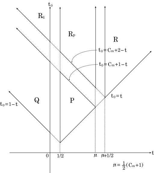
Figure 1: The subspaces $P$, $Q$, $R_{p}$, $R_{q}$ and $R$ are shown on the $t$-$t_{0}$ plane.

For the preparation of the main discussion, first, we make a list of the relations. The relations (I.3.7a) and (I.3.8c) are rewritten as

$${\hat{T}}=\frac{1}{2}\left(C_{m}+1\right)-{\hat{\cal S}}\ ,\qquad{\hat{T}}_{0}=\frac{1}{2}\left(C_{m}+1\right)+{\hat{\cal S}}_{0}\ ,$$ (2.1)

$${\rm i.e.,}\quad t=\frac{1}{2}\left(C_{m}+1\right)-s\ ,\qquad t_{0}=\frac{1}{2}\left(C_{m}+1\right)+s_{0}\ .$$ (2.2)

The relations (I.3.9a) and (I.3.9b) are rewritten as

$${\hat{\cal S}}_{+}={\hat{a}}^{*}{\hat{b}}^{*}\cdot\left(\sqrt{C_{m}+1-{\hat{\cal S}}+{\hat{\cal S}}_{0}+\epsilon}\right)^{-1}\cdot\sqrt{{\hat{\cal S}}-{\hat{\cal S}}_{0}}\ ,$$ (2.3a)

$${\hat{\cal S}}_{-}=\sqrt{{\hat{\cal S}}-{\hat{\cal S}}_{0}}\cdot\left(\sqrt{C_{m}+1-{\hat{\cal S}}+{\hat{\cal S}}_{0}+\epsilon}\right)^{-1}\cdot{\hat{b}}{\hat{a}}\ .$$ (2.3b)

The minimum weight state denoted by $|{s,\sigma}\rangle$ obeys the conditions

$${\hat{\cal S}}_{-}|{s,\sigma}\rangle=0\ ,\qquad{\rm i.e.,}\qquad{\hat{b}}{\hat{a}}|{s,\sigma}\rangle=0\ ,$$ (2.4)

$${\hat{\cal S}}|{s,\sigma}\rangle=s|{s,\sigma}\rangle\ ,\qquad{\hat{\cal S}}_{0}|{s,\sigma}\rangle=\sigma|{s,\sigma}\rangle\ .$$ (2.5)

The relations (2.4) and (2.5) with (2.3b) give us

$$P\ ;\ \ |{s,\sigma}\rangle=({\hat{b}}^{*})^{C_{m}-2s}|{0}\rangle\ ,\qquad\sigma=-s\ ,$$ (2.6)

$$Q\ ;\ \ |{s,\sigma}\rangle=({\hat{a}}^{*})^{2s-C_{m}}|{0}\rangle\ ,\qquad\sigma=s-C_{m}\ .$$ (2.7)

Here, the normalization constants are omitted. Since $C_{m}-2s\geq 0$ and $2s-C_{m}\geq 1$, we have the inequalities

$$P\ ;\quad s\leq\frac{1}{2}C_{m}\ ,$$ (2.8)

$$Q\ ;\quad s\geq\frac{1}{2}\left(C_{m}+1\right)\ .$$ (2.9)

By operating ${\hat{\cal S}}_{+}$ successively on the state $|{s,\sigma}\rangle$, we are able to obtain the eigenstate of ${\hat{\cal S}}$ and ${\hat{\cal S}}_{0}$ with the eigenvalues $s$ and $s_{0}$, respectively, in the form

$$P\ ;\ \ |{s,s_{0}}\rangle=\left({\hat{\cal S}}_{+}\right)^{s+s_{0}}|{s,-s}\rangle\ ,$$ (2.10)

$$Q\ ;\ \ |{s,s_{0}}\rangle=\left({\hat{\cal S}}_{+}\right)^{C_{m}-s+s_{0}}|{s,s-C_{m}}\rangle\ .$$ (2.11)

Here, the normalization constants are omitted. Since $s+s_{0}\geq 0$ and $C_{m}-s+s_{0}\geq 0$, we have

$$P\ ;\ \ s_{0}\geq-s\ ,$$ (2.12)

$$Q\ ;\ \ s_{0}\geq s-C_{m}\ .$$ (2.13)

Our system has the maximum weight state denoted as $|{s,\sigma_{m}}\rangle$. It satisfies

$${\hat{\cal S}}_{+}|{s,\sigma_{m}}\rangle=0\ ,\qquad{\rm i.e.,}\qquad\sqrt{{\hat{\cal S}}-{\hat{\cal S}}_{0}}\ |{s,\sigma_{m}}\rangle=0\ ,$$ (2.14)

$${\hat{\cal S}}|{s,\sigma_{m}}\rangle=s|{s,\sigma_{m}}\rangle\ ,\qquad{\hat{\cal S}}_{0}|{s,\sigma_{m}}\rangle=\sigma_{m}|{s,\sigma_{m}}\rangle\ .$$ (2.15)

The relation (2.14) and (2.15) give us

$$P\ \ {\rm and}\ \ Q\ ;\quad\sigma_{m}=s\ .$$ (2.16)

Then, the quantum number $s_{0}$ satisfies

$$P\ ;\ \ -s\leq s_{0}\leq s\ ,\qquad{\rm i.e.,}\qquad s_{0}=-s,\ -s+1,\cdots,\ s-1,\ s,$$ (2.17)

$$Q\ ;\ \ s-C_{m}\leq s_{0}\leq s\ ,\qquad{\rm i.e.,}\qquad s_{0}=s-C_{m},\ s-C_{m}+1,\cdots,\ s-1,\ s.\qquad$$ (2.18)

We can see that ${\hat{\cal S}}_{\pm,0}$ obey the $su(2)$-algebra in $P$, but do not in $Q$. The relations (2.8) and (2.9) teach us that the upper and the lower limit of $s$ in $P$ and in $Q$, respectively, exist. Therefore, it may be interesting to show the lower and the upper limit of $s$ in $P$ and in $Q$, respectively. For this task, the first of the relation (2.2) is useful. As can be seen in Fig.1, the quantum number $t$ in $P$ and in $Q$ obeys

$$P\ ;\ \ t=1/2,\ 1,\ 3/2,\cdots,\ \mu-1/2,\ \mu,$$ (2.19)

$$Q\ ;\ \ t=0,-1/2,\ -1,\cdots,\ -\infty.$$ (2.20)

Combining the relations (2.19) and (2.20) with the relation (2.2), we have the following:

$$P\ ;\ \ s=\frac{1}{2}C_{m},\ \frac{1}{2}(C_{m}-1),\ \frac{1}{2}(C_{m}-2),\cdots,\ \frac{1}{2},\ 0,$$ (2.21)

$$Q\ ;\ \ s=\frac{1}{2}(C_{m}+1),\ \frac{1}{2}(C_{m}+2),\ \frac{1}{2}(C_{m}+3),\cdots,\ \infty.$$ (2.22)

In $P$, there exists the lower limit $s=0$, but in $Q$, the upper limit is $\infty$.

Next, we investigate the commutation relations for ${\hat{\cal S}}_{\pm,0}$ and ${\hat{\cal S}}$. For the above discussion, the following played a central role:

$$[\ {\hat{\cal S}}_{0}\ ,\ {\hat{\cal S}}_{\pm}\ ]=\pm{\hat{\cal S}}_{\pm}\ ,\qquad[\ {\hat{\cal S}}\ ,\ {\hat{\cal S}}_{\pm,0}\ ]=0\ .$$ (2.23)

Of course, the above relation is useful both in $P$ and in $Q$. Our problem is to investigate the relation $[\ {\hat{\cal S}}_{+}\ ,\ {\hat{\cal S}}_{-}\ ]$. Direct calculation gives us the form

$$[\ {\hat{\cal S}}_{+}\ ,\ {\hat{\cal S}}_{-}\ ]=2\left({\hat{\cal S}}_{0}+\Delta{\hat{\cal S}}_{0}\right)\ ,$$ (2.24)

$$\Delta{\hat{\cal S}}_{0}=\Delta{\hat{\cal S}}_{0}^{(+)}-\Delta{\hat{\cal S}}_{0}^{(-)}\ ,$$

$$\Delta{\hat{\cal S}}_{0}^{(+)}=\frac{\epsilon}{2}\frac{\left({\hat{T}}_{0}-{\hat{T}}+1\right)\left(C_{m}+1-{\hat{T}}_{0}-{\hat{T}}\right)}{{\hat{T}}_{0}+{\hat{T}}+\epsilon}\ ,$$

$$\Delta{\hat{\cal S}}_{0}^{(-)}=\frac{\epsilon}{2}\frac{\left({\hat{T}}_{0}-{\hat{T}}\right)\left(C_{m}+2-{\hat{T}}_{0}-{\hat{T}}\right)}{{\hat{T}}_{0}+{\hat{T}}-1+\epsilon}\ .$$ (2.25)

Apparently, $[\ {\hat{\cal S}}_{+}\ ,\ {\hat{\cal S}}_{-}\ ]$ does not satisfy the commutation relation in the $su(2)$-algebra. As can be seen in Fig.1, $t_{0}$ and $t$ obey the inequality $t_{0}+t>0$ both in $P$ and in $Q$. It indicates that the term $({\hat{T}}_{0}+{\hat{T}})$ appearing in the denominator of $\Delta{\hat{\cal S}}_{0}^{(+)}$ is positive-definite and, then, we have

$$P\ {\rm and}\ Q\ ;\ \ \Delta{\hat{\cal S}}_{0}^{(+)}\longrightarrow 0\ ,\quad(\epsilon\rightarrow 0)\ .$$ (2.26)

In the case $\Delta{\hat{\cal S}}_{0}^{(-)}$, it may be necessary to investigate if the operator $({\hat{T}}_{0}+{\hat{T}}-1)$ appearing in the denominator is positive-definite or not. For this aim, the condition $t_{0}+t-1=0$ should be examined: In $P$, $t_{0}=t=1/2$ and in $Q$, $t_{0}=-t+1$ $(t\leq 0)$. Figure 1 gives us these relations. We notice the term $({\hat{T}}_{0}-{\hat{T}})$ appearing in the numerator of $\Delta{\hat{\cal S}}_{0}^{(-)}$. In this case, $t_{0}-t=1/2-1/2=0$. Therefore, the following result is derived:

$$P\ ;\ \ \Delta{\hat{\cal S}}_{0}^{(-)}\longrightarrow 0\ ,\quad(\epsilon\rightarrow 0)\ .$$ (2.27)

On the other hand, there does not exist the term which leads to $\Delta{\hat{\cal S}}_{0}^{(-)}\rightarrow 0$, $(\epsilon\rightarrow 0)$. Therefore, we have

$$Q\ ;\ \ \Delta{\hat{\cal S}}_{0}^{(-)}\longrightarrow\frac{1}{2}\left({\hat{T}}_{0}-{\hat{T}}\right)\left(C_{m}+2-{\hat{T}}_{0}-{\hat{T}}\right)\cdot{\hat{Q}}_{0}\ ,\quad(\epsilon\rightarrow 0)\ ,$$ (2.29)

$${\hat{Q}}_{0}=\sum_{t\leq 0}|{t,t_{0}=-t+1}\rangle\langle{t,t_{0}=-t+1}|$$

$$\quad\ \ =\sum_{s\geq 1/2\cdot(C_{m}+1)}|{s,\sigma}\rangle\langle{s,\sigma}|\ .\quad(\sigma=s-C_{m})$$

For the operator ${\hat{\mib{\cal S}}}^{2}$, we have

$${\hat{\mib{\cal S}}}^{2}={\hat{\cal S}}\left({\hat{\cal S}}+1\right)-\frac{1}{2}\left(\Delta{\hat{\cal S}}_{0}^{(+)}+\Delta{\hat{\cal S}}_{0}^{(-)}\right)\ .$$ (2.30)

Therefore, for $\epsilon\rightarrow 0$, ${\hat{\mib{\cal S}}}^{2}$ is expressed in the form

$$P\ ;\ \ {\hat{\mib{\cal S}}}^{2}\longrightarrow{\hat{\cal S}}\left({\hat{\cal S}}+1\right)\ ,$$ (2.31)

$$Q\ ;\ \ {\hat{\mib{\cal S}}}^{2}\longrightarrow{\hat{\cal S}}\left({\hat{\cal S}}+1\right)-\frac{1}{2}\left({\hat{T}}_{0}-{\hat{T}}\right)\left(C_{m}+2-{\hat{T}}_{0}-{\hat{T}}\right)\cdot{\hat{Q}}_{0}\ .$$ (2.32)

The above consideration teaches us that ${\hat{\cal S}}_{\pm,0}$ obey the $su(2)$-algebra in $P$, but they does not obey the $su(2)$-algebra in $Q$. It may be permitted to call the algebra in $Q$ the pseudo $su(2)$-algebra. With the use of the commutation relation (2.24), we can determine the normalization constants of the states (2.6) and (2.7). For this aim, the following formula is useful:

$$\langle{s,\sigma}|\left({\hat{\cal S}}_{-}\right)^{n}\cdot\left({\hat{\cal S}}_{+}\right)^{n}|{s,\sigma}\rangle=(-)^{n}n!\frac{\Gamma(2\sigma+n)}{\Gamma(2\sigma)}\langle{s,\sigma}|s,\sigma\rangle\ .$$ (2.33)

Combining the formula (2.33) with the relations (2.6), (2.7), (2.10) and (2.11), we can determine the norms of the states (2.10) and (2.11) in the following form :

$$P\ ;\ \ \langle{s,s_{0}}|s,s_{0}\rangle=\frac{(2s)!(s+s_{0})!}{(s-s_{0})!}\cdot(C_{m}-2s)!\ ,$$ (2.34)

$$Q\ ;\ \ \langle{s,s_{0}}|s,s_{0}\rangle=(-)^{C_{m}-s+s_{0}}\frac{(C_{m}-s+s_{0})!\Gamma(s+s_{0}-C_{m})}{\Gamma(2(s-C_{m}))}\cdot(2s-C_{m})!\ .$$ (2.35)

With the aid of the relations (2.34) and (2.35), we are able to obtain the normalized $|{s,s_{0}}\rangle$. Clearly, the relation (2.34) is the same as that in the $su(2)$-algebra. Of course, $(C_{m}-2s)!$ is derived under the minimum weight state (2.6). The above is the supplementary explanation of our boson representation of the $su(2)$-algebra. Certainly, in $P$, our representation obeys the $su(2)$-algebra. Concerning the subspaces $R_{p}$, $R_{q}$ and $R$, we will discuss in §6.

3 Raising and lowering operator for the magnitude of the $su(2)$-spin

In this section, we will discuss a role of the original Schwinger representation (I.3.1) in our present one. It is shown that the operators ${\hat{S}}_{+}$ and ${\hat{S}}_{-}$ play the role of the raising and the lowering operator for the magnitude of the $su(2)$-spin, respectively. First, we notice that the relation between $(t,t_{0})$ and $(s,s_{0})$ is given as

$$t=\frac{1}{2}(C_{m}+1)-s\ ,\qquad t_{0}=\frac{1}{2}(C_{m}+1)+s_{0}\ .$$ (3.1)

The form (3.1) is derived from the relations (I.3.7a) and (I.3.8c) with the relation (I.2.16a). The space is characterized by the conditions $t\leq t_{0}\leq C_{m}+1-t$ and $1/2\leq t\leq\mu$, which leads us to the following conditions for $(s,s_{0})$:

$$-s\leq s_{0}\leq s\ ,$$ (3.2a)

$$0\leq s\leq\frac{1}{2}C_{m}\ .$$ (3.2b)

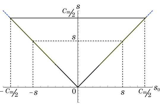
Figure 2: The condition (3.2) is depicted on the $s$-$s_{0}$ plane.

The condition (3.2) can be shown in Fig.2. With the use of the relation (3.1), the state $|{t,t_{0}}\rangle$ in $P$ can be expressed in the form

$$|{t,t_{0}}\rangle=\frac{1}{\sqrt{(t_{0}-t)!(t_{0}+t-1)!}}({\hat{a}}^{*})^{t_{0}-t}({\hat{b}}^{*})^{t_{0}+t-1}|{0}\rangle$$ (3.3)

$$= |{s,s_{0}}\rangle=\frac{1}{\sqrt{(s+s_{0})!(C_{m}-s+s_{0})!}}({\hat{a}}^{*})^{s+s_{0}}({\hat{b}}^{*})^{C_{m}-s+s_{0}}|{0}\rangle\ .$$

The state $|\!|{s,s_{0}}\rangle$ in the Schwinger representation is given as

$$|\!|{s,s_{0}}\rangle=\frac{1}{\sqrt{(s+s_{0})!(s-s_{0})!}}({\hat{a}}^{*})^{s+s_{0}}({\hat{b}}^{*})^{s-s_{0}}|{0}\rangle\ .$$ (3.4)

The state (3.3) gives us the relation

$${\hat{S}}_{+}|{s,s_{0}}\rangle={\hat{a}}^{*}{\hat{b}}|{s,s_{0}}\rangle=\sqrt{(s+s_{0}+1)(C_{m}-s+s_{0})}|{s+1,s_{0}}\rangle\ ,$$ (3.5a)

$${\hat{S}}_{-}|{s,s_{0}}\rangle={\hat{b}}^{*}{\hat{a}}|{s,s_{0}}\rangle=\sqrt{(s+s_{0})(C_{m}-s+s_{0}+1)}|{s-1,s_{0}}\rangle\ ,$$ (3.5b)

$${\hat{S}}_{0}|{s,s_{0}}\rangle=\frac{1}{2}({\hat{a}}^{*}{\hat{a}}-{\hat{b}}^{*}{\hat{b}})|{s,s_{0}}\rangle=\left(s-\frac{1}{2}C_{m}\right)|{s,s_{0}}\rangle\ .$$ (3.5c)

Here, ${\hat{S}}_{\pm,0}$ denote the generators of the $su(2)$-algebra in the Schwinger representation. In the relations (3.5a) and (3.5b), we can see that ${\hat{S}}_{+}$ and ${\hat{S}}_{-}$ play the role of the raising and the lowering operator, respectively, not for $s_{0}$ but for $s$. However, we must notice the case $s=C_{m}/2$. Operation of ${\hat{S}}_{+}$ on the state $|{C_{m}/2,s_{0}}\rangle$ should vanish, because $C_{m}/2+1$ does not belong to the space $P$. In order to overcome this trouble, we define the following operators:

$${\hat{\Sigma}}_{+}={\hat{S}}_{+}\!\cdot\!\sqrt{\frac{1}{2}C_{m}-{\hat{\cal S}}}\!\cdot\!\left(\sqrt{\frac{1}{2}C_{m}-{\hat{\cal S}}+\epsilon}\right)^{-1}\ ,$$

(3.6a)

$${\hat{\Sigma}}_{-}=\left(\sqrt{\frac{1}{2}C_{m}-{\hat{\cal S}}+\epsilon}\right)^{-1}\!\!\cdot\!\sqrt{\frac{1}{2}C_{m}-{\hat{\cal S}}}\cdot{\hat{S}}_{-},$$

(3.6b)

$${\hat{\Sigma}}_{0}={\hat{\cal S}}-\frac{1}{2}C_{m}\ .$$ (3.6c)

Then, we have

$${\hat{\Sigma}}_{+}|{C_{m}/2,s_{0}}\rangle=0\ .$$ (3.7)

The above indicates that the state $|{C_{m}/2,s_{0}}\rangle$ is the maximum weight state.

The commutation relations for ${\hat{\Sigma}}_{\pm,0}$ are given in the form

$$[\ {\hat{\Sigma}}_{0}\ ,\ {\hat{\Sigma}}_{\pm}\ ]=\pm{\hat{\Sigma}}_{\pm}\ ,$$ (3.8)

$$[\ {\hat{\Sigma}}_{+}\ ,\ {\hat{\Sigma}}_{-}\ ]=2\left({\hat{\Sigma}}_{0}+\Delta{\hat{\Sigma}}_{0}\right)\ ,$$ (3.9)

$$\Delta{\hat{\Sigma}}_{0}=\frac{\epsilon}{2}\frac{\left({\hat{\cal S}}_{0}+{\hat{\cal S}}+1\right)\left({\hat{\cal S}}_{0}+C_{m}-{\hat{\cal S}}\right)}{\frac{1}{2}C_{m}-{\hat{\cal S}}+\epsilon}\ .$$ (3.10)

The operator ${\hat{\mib{\Sigma}}}^{2}$ corresponding to the Casimir operator of the $su(2)$-algebra is given as

$${\hat{\mib\Sigma}}^{2} = {\hat{\Sigma}}_{0}^{2}+\frac{1}{2}\left({\hat{\Sigma}}_{-}{\hat{\Sigma}}_{+}+{\hat{\Sigma}}_{+}{\hat{\Sigma}}_{-}\right)$$ (3.11)

$$= {\hat{\Sigma}}\left({\hat{\Sigma}}+1\right)-\left(\Delta{\hat{\Sigma}}_{0}^{(+)}+\Delta{\hat{\Sigma}}_{0}^{(-)}\right)\ ,$$

$${\hat{\Sigma}} = {\hat{\cal S}}_{0}+\frac{1}{2}C_{m}\ .$$ (3.12)

We can see that the set ${\hat{\Sigma}}_{\pm,0}$ forms a kind of the pseudo $su(2)$-algebra.

Thus, we could learn the existence of the raising and the lowering operator for the magnitude of the $su(2)$-spin. With the use of the operator ${\hat{\Sigma}}_{+}$ and ${\hat{\cal S}}_{\pm}$, we can express the state $|{s,s_{0}}\rangle$ in the form

$$|{s,s_{0}}\rangle=\left({\hat{\cal S}}_{+}\right)^{s+s_{0}}|{s,-s}\rangle\ ,$$ (3.13a)

$$|{s,-s}\rangle=\left({\hat{\cal S}}_{-}{\hat{\Sigma}}_{+}\right)^{s-\rho}|{\rho,-\rho}\rangle\ ,$$ (3.13b)

$$|{\rho,-\rho}\rangle=({\hat{b}}^{*})^{C_{m}-2\rho}|{0}\rangle\ .\qquad\left(\rho=0\ {\rm and}\ \frac{1}{2}\right)$$ (3.13c)

In the above relations, we omitted the normalization constants. If $\rho=0$ and $1/2$, $s$ become integer and half-integer, respectively. However, we must remark that the above idea is not proper to our representation. In the case of the Schwinger representation, we obtain the state $|\!|{s,s_{0}}\rangle$ by replacing ${\hat{\cal S}}_{\pm}$, ${\hat{\Sigma}}_{+}$ and $|{\rho,-\rho}\rangle$ with ${\hat{S}}_{\pm}$, ${\hat{T}}_{+}$ and $|\!|{\rho,-\rho}\rangle=({\hat{b}}^{*})^{\rho}|{0}\rangle$.

4 Connection to the Holstein-Primakoff representation

It may be interesting to show how the Holstein-Primakoff representation [3] can be derived from our representation (I.3.9). The three $su(2)$-generators (I.3.9) are rewritten to the following forms:

$${\hat{\cal S}}_{+}={\hat{a}}^{*}{\hat{\beta}}^{*}\cdot\sqrt{2{\hat{\cal S}}-{\hat{a}}^{*}{\hat{a}}}\ ,\qquad{\hat{\cal S}}_{-}=\sqrt{2{\hat{\cal S}}-{\hat{a}}^{*}{\hat{a}}}\cdot{\hat{\beta}}{\hat{a}}\ ,\qquad{\hat{\cal S}}_{0}={\hat{a}}^{*}{\hat{a}}-{\hat{\cal S}}\ .$$ (4.1)

Here, (${\hat{\beta}},{\hat{\beta}}^{*})$ is defined in the form

$${\hat{\beta}}=\left(\sqrt{{\hat{b}}^{*}{\hat{b}}+1+\epsilon}\right)^{-1}\cdot{\hat{b}}\ ,\qquad{\hat{\beta}}^{*}={\hat{b}}^{*}\cdot\left(\sqrt{{\hat{b}}^{*}{\hat{b}}+1+\epsilon}\right)^{-1}\ .$$ (4.2)

Further, for the above rewriting, we used the relation

$$C_{m}-{\hat{b}}^{*}{\hat{b}}=2{\hat{\cal S}}-{\hat{a}}^{*}{\hat{a}}\ .$$ (4.3)

The relation (4.3) comes from the form (I.3.10). Any of $({\hat{\beta}},{\hat{\beta}}^{*})$ connects with any of $({\hat{a}},{\hat{a}}^{*})$ and we have the relation

$${\hat{\beta}}{\hat{\beta}}^{*}=1-\frac{\epsilon}{{\hat{b}}^{*}{\hat{b}}+1+\epsilon}\rightarrow 1\ ,\quad(\epsilon\rightarrow 0)$$ (4.4a)

$${\hat{\beta}}^{*}{\hat{\beta}}=1-\frac{\epsilon}{{\hat{b}}^{*}{\hat{b}}+\epsilon}\ .$$ (4.4b)

Therefore, $[{\hat{\beta}}\ ,\ {\hat{\beta}}^{*}]$ is given as

$$[\ {\hat{\beta}}\ ,\ {\hat{\beta}}^{*}\ ]=\frac{\epsilon}{{\hat{b}}^{*}{\hat{b}}+\epsilon}\ .$$ (4.5)

The operator $[{\hat{\beta}}\ ,\ {\hat{\beta}}^{*}]$ plays a role of projection operator and, for the state (3.3), we have

$$[\ {\hat{\beta}}\ ,\ {\hat{\beta}}^{*}\ ]|{s,s_{0}}\rangle=\frac{\epsilon}{C_{m}-s+s_{0}+\epsilon}|{s,s_{0}}\rangle=\delta_{s-s_{0},C_{m}}|{s,s_{0}}\rangle\ .\qquad(\epsilon\rightarrow 0)$$ (4.6)

Our boson representation is given in the space $P$ in Fig.1 or Fig.2 and, then, $\delta_{s-s_{0},C_{m}}$ takes the value 1 in the case

$$s=s_{\rm max}=\frac{C_{m}}{2}\ ,\qquad s_{0}=-s_{\rm max}=-\frac{C_{m}}{2}\ ,\qquad\delta_{s-s_{0},C_{m}}|{s,s_{0}}\rangle=|{\frac{C_{m}}{2},-\frac{C_{m}}{2}}\rangle\ .$$ (4.7a)

In any other case, we have

$$\delta_{s-s_{0},C_{m}}|{s,s_{0}}\rangle=0\ .$$ (4.7b)

With the use of $({\hat{\beta}},{\hat{\beta}}^{*})$, we define the operator $({\hat{c}},{\hat{c}}^{*})$:

$${\hat{c}}={\hat{\beta}}{\hat{a}}\ (={\hat{a}}{\hat{\beta}})\ ,\qquad{\hat{c}}^{*}={\hat{a}}^{*}{\hat{\beta}}^{*}\ (={\hat{\beta}}^{*}{\hat{a}}^{*})\ .$$ (4.8)

The operator $({\hat{c}},{\hat{c}}^{*})$ satisfies the relation

$${\hat{c}}{\hat{c}}^{*} = {\hat{a}}{\hat{\beta}}{\hat{\beta}}^{*}{\hat{a}}^{*}={\hat{a}}{\hat{a}}^{*}\ ,$$ (4.9a)

$${\hat{c}}^{*}{\hat{c}} = {\hat{a}}^{*}{\hat{\beta}}^{*}{\hat{\beta}}{\hat{a}}={\hat{a}}^{*}{\hat{a}}\cdot({\hat{\beta}}^{*}{\hat{\beta}})={\hat{a}}^{*}{\hat{a}}-{\hat{a}}^{*}{\hat{a}}[\ {\hat{\beta}}\ ,\ {\hat{\beta}}^{*}\ ]$$ (4.9b)

$$= {\hat{a}}^{*}{\hat{a}}-\left({\hat{\cal S}}+{\hat{\cal S}}_{0}\right)[\ {\hat{\beta}}\ ,\ {\hat{\beta}}^{*}\ ]\rightarrow{\hat{a}}^{*}{\hat{a}}\ .\qquad(\epsilon\rightarrow 0)$$

We notice that $({\hat{\cal S}}+{\hat{\cal S}}_{0})[{\hat{\beta}},{\hat{\beta}}^{*}]|{C_{m}/2,-C_{m}/2}\rangle=(C_{m}/2-C_{m}/2)|{C_{m}/2,-C_{m}/2}\rangle$ and for any other case, $[{\hat{\beta}},{\hat{\beta}}^{*}]|{s,s_{0}}\rangle=0$. Therefore, $({\hat{c}},{\hat{c}}^{*})$ is boson operator:

$$[\ {\hat{c}}\ ,\ {\hat{c}}^{*}\ ]=[\ {\hat{a}}\ ,\ {\hat{a}}^{*}\ ]=1\ ,\qquad{\hat{c}}|{0}\rangle={\hat{b}}|{0}\rangle={\hat{a}}|{0}\rangle=0\ .$$ (4.10)

Further, we obtain the relation

$$[\ {\hat{c}}\ ,\ {\hat{\cal S}}\ ]=[\ {\hat{c}}^{*}\ ,\ {\hat{\cal S}}\ ]=0\ .$$ (4.11)

With the use of the relations obtained above, ${\hat{\cal S}}_{\pm,0}$ can be rewritten to the form

$${\hat{\cal S}}_{+}={\hat{c}}^{*}\sqrt{2{\hat{\cal S}}-{\hat{c}}^{*}{\hat{c}}}\ ,\qquad{\hat{\cal S}}_{-}=\sqrt{2{\hat{\cal S}}-{\hat{c}}^{*}{\hat{c}}}\ {\hat{c}}\ ,\qquad{\hat{\cal S}}_{0}={\hat{c}}^{*}{\hat{c}}-{\hat{\cal S}}\ .$$ (4.12)

By setting $s+s_{0}=n$ in the state (3.3), we have

$$f\left({\hat{\cal S}},{\hat{c}}^{*}{\hat{c}}\right)|{s,s_{0}}\rangle=f(s,n)|{s,s_{0}}\rangle=f(s,{\hat{c}}^{*}{\hat{c}})|{s,s_{0}}\rangle\ .$$ (4.13)

Therefore, in the space spanned by $|{s,s_{0}}\rangle$ $(s_{0}=-s,\ -s+1,\cdots,\ s-1,\ s)$, the expression (4.12) can be regarded as

$${\hat{S}}_{+}={\hat{c}}^{*}\sqrt{2s-{\hat{c}}^{*}{\hat{c}}}_{,}\qquad{\hat{S}}_{-}=\sqrt{2s-{\hat{c}}^{*}{\hat{c}}}\ {\hat{c}}\ ,\qquad{\hat{S}}_{0}={\hat{c}}^{*}{\hat{c}}-s\ .$$ (4.14)

The above is nothing but the Holstein-Primakoff representation. In Ref.4, we discussed an idea how to derive the Holstein-Primakoff representation from the Schwinger one. In this case, much more lengthy discussion was necessary. The main reason may be attributed to the fact that the operator corresponding to $({\hat{c}},{\hat{c}}^{*})$ does not satisfy the simple boson commutation relation. The state (3.3) can be rewritten to

$$|{s,s_{0}}\rangle~{}\frac{1}{\sqrt{(s+s_{0})!}}({\hat{c}}^{*})^{s+s_{0}}|{s,-s}\rangle\ ,$$ (4.15)

$$|{s,-s}\rangle=\frac{1}{\sqrt{(C_{m}-2s)!}}({\hat{b}}^{*})^{C_{m}-2s}|{0}\rangle\ (=|{\phi}\rangle)\ .$$ (4.16)

Clearly, ${\hat{c}}$ satisfies

$${\hat{c}}|{\phi}\rangle=0\ .$$ (4.17)

Since the state $|{\phi}\rangle$ is the vacuum of ${\hat{c}}$, we have the orthogonal set:

$$|{n}\rangle=\frac{1}{\sqrt{n!}}({\hat{c}}^{*})^{n}|{\phi}\rangle\ .\qquad(n=0,\ 1,\cdots,\ 2s)$$ (4.18)

The above is the connection to the Holstein-Primakoff representation.

5 Connection to the Schwinger representation

In this section, we will discuss how the Schwinger boson representation is connected to the present one. The three generators ${\hat{\cal S}}_{\pm,0}$ and ${\hat{\cal S}}$ given in the relations (I.3.9) and (I.3.10) are rewritten to the form

$${\hat{\cal S}}_{+}={\hat{a}}^{*}{\hat{\beta}}^{*}\cdot\sqrt{C_{m}-{\hat{b}}^{*}{\hat{b}}}\ ,\quad{\hat{\cal S}}_{-}=\sqrt{C_{m}-{\hat{b}}^{*}{\hat{b}}}\cdot{\hat{\beta}}{\hat{a}}\ ,\quad{\hat{\cal S}}_{0}=\frac{1}{2}({\hat{a}}^{*}{\hat{a}}-(C_{m}-{\hat{b}}^{*}{\hat{b}}))\ ,\qquad$$ (5.1)

$${\hat{\cal S}}=\frac{1}{2}({\hat{a}}^{*}{\hat{a}}+(C_{m}-{\hat{b}}^{*}{\hat{b}}))\ .$$ (5.2)

Here, $({\hat{\beta}},{\hat{\beta}}^{*})$ is given in the relation (4.2). In order to rewrite the expressions (5.1) and (5.2), we introduce the operator $({\breve{b}},{\breve{b}}^{*})$ in the form

$${\breve{b}}={\hat{\beta}}^{*}\sqrt{C_{m}-{\hat{b}}^{*}{\hat{b}}}\ ,\qquad{\breve{b}}^{*}=\sqrt{C_{m}-{\hat{b}}^{*}{\hat{b}}}\ {\hat{\beta}}\ .$$ (5.3)

With the use of $({\breve{b}},{\breve{b}}^{*})$, ${\hat{\cal S}}_{\pm,0}$ and ${\hat{\cal S}}$ can be expressed as

$${\breve{\cal S}}_{+}={\hat{a}}^{*}{\breve{b}}\ ,\qquad{\breve{\cal S}}_{-}={\breve{b}}^{*}{\hat{a}}\ ,\qquad{\breve{\cal S}}_{0}=\frac{1}{2}({\hat{a}}^{*}{\hat{a}}-{\breve{b}}^{*}{\breve{b}})\ ,$$ (5.4)

$${\breve{\cal S}}=\frac{1}{2}({\hat{a}}^{*}{\hat{a}}+{\breve{b}}^{*}{\breve{b}})\ .$$ (5.5)

Here, it should be noted that we rewrite ${\hat{\cal S}}_{\pm,0}$ and ${\hat{\cal S}}$ shown in the relations (5.1) and (5.2), in the forms (5.4) and (5.5) and, then, ${\breve{\cal S}}_{\pm,0}={\hat{\cal S}}_{\pm,0}$ and ${\breve{\cal S}}={\hat{\cal S}}$. If $({\breve{b}},{\breve{b}}^{*})$ is boson operator, the expression (5.4) (and (5.5)) reduce to the Schwinger boson representation (I.3.1) (and (I.3.2)). Therefore, it may be interesting to investigate the condition, under which $({\breve{b}},{\breve{b}}^{*})$ can be regarded as boson. For this aim, we must calculate the commutation relation $[{\breve{b}},{\breve{b}}^{*}]$, the result of which is as follows:

$$[\ {\breve{b}}\ ,\ {\breve{b}}^{*}\ ] = 1-(C_{m}+1-{\hat{b}}^{*}{\hat{b}})[\ {\hat{\beta}}\ ,\ {\hat{\beta}}^{*}\ ]=1-(C_{m}+1-{\hat{b}}^{*}{\hat{b}})\frac{\epsilon}{{\hat{b}}^{*}{\hat{b}}+\epsilon}$$ (5.6)

$$= 1-\frac{\epsilon({\breve{b}}^{*}{\breve{b}}+1)}{C_{m}-{\breve{b}}^{*}{\breve{b}}+\epsilon}\ .$$

Here, we used the relation

$${\breve{b}}{\breve{b}}^{*}=(C_{m}+1-{\breve{b}}^{*}{\breve{b}}){\hat{\beta}}^{*}{\hat{\beta}}\ ,\qquad{\breve{b}}^{*}{\breve{b}}=C_{m}-{\hat{b}}^{*}{\hat{b}}\ .$$ (5.7)

In the relation (5.6), we can see that if $C_{m}\rightarrow\infty$, $({\breve{b}},{\breve{b}}^{*})$ may be regarded as boson.

In order to clarify the above-mentioned situation, we consider orthogonal set constructed by ${\breve{b}}^{*}$. First, we introduce the state $|{0}\rangle\!\rangle$ defined as

$$|{0}\rangle\!\rangle=({\hat{\beta}}^{*})^{C_{m}}|{0}\rangle=\frac{1}{\sqrt{C_{m}!}}({\hat{b}}^{*})^{C_{m}}|{0}\rangle\ .$$ (5.8)

The state $|{0}\rangle\!\rangle$ is the vacuum for ${\breve{b}}$:

$${\breve{b}}|{0}\rangle\!\rangle={\hat{\beta}}^{*}\sqrt{C_{m}-{\hat{b}}^{*}{\hat{b}}}\cdot\frac{1}{\sqrt{C_{m}!}}({\hat{b}}^{*})^{C_{m}}|{0}\rangle=0\ .$$ (5.9)

Then, we define the state $|{n}\rangle\!\rangle$ in the form

$$|{n}\rangle\!\rangle=({\hat{\beta}}^{*})^{C_{m}-n}|{0}\rangle=\frac{1}{\sqrt{(C_{m}-n)!}}({\hat{b}}^{*})^{C_{m}-n}|{0}\rangle\ .\qquad(n=0,\ 1,\ 2,\cdots,\ C_{m})$$ (5.10)

It can be proved that $|{n}\rangle\!\rangle$ is expressed as

$$|{n}\rangle\!\rangle=\frac{1}{\sqrt{n!}}({\breve{b}}^{*})^{n}|{0}\rangle\!\rangle\ .$$ (5.11)

If $n=C_{m}$, we have the following relation:

$${\breve{b}}^{*}|{C_{m}}\rangle\!\rangle=\sqrt{C_{m}-{\hat{b}}^{*}{\hat{b}}}\ {\hat{\beta}}|{0}\rangle=0\ .$$ (5.12)

It may be interesting to see that the operation of ${\breve{b}}^{*}$ on $|{C_{m}}\rangle\!\rangle$ vanishes. Therefore, if $C_{m}\rightarrow\infty$, the relation (5.12) becomes meaningless. The commutation relation (5.6) gives us the following:

$$[\ {\breve{b}}\ ,\ {\breve{b}}^{*}\ ]|{n}\rangle\!\rangle=|{n}\rangle\!\rangle\ ,\qquad(n=0,\ 1,\ 2,\cdots,\ C_{m}-1)$$ (5.13a)

$$[\ {\breve{b}}\ ,\ {\breve{b}}^{*}\ ]|{C_{m}}\rangle\!\rangle=-C_{m}|{C_{m}}\rangle\!\rangle\ .$$ (5.13b)

In the relation (5.13b), we have ${\breve{b}}{\breve{b}}^{*}|{C_{m}}\rangle\!\rangle=0$ and ${\breve{b}}^{*}{\breve{b}}|{C_{m}}\rangle\!\rangle=C_{m}|{C_{m}}\rangle\!\rangle$, which comes from the relation (5.12). From the above argument, we can conclude that if $C_{m}\rightarrow\infty$, $({\breve{b}},{\breve{b}}^{*})$ can be regarded as boson operator. In this connection, we mention that if $C_{m}=1$, $({\breve{b}},{\breve{b}}^{*})$ becomes fermion operator.

Under the above consideration, we investigate the eigenvalue problem for ${\breve{\cal S}}_{\pm,0}$ and ${\breve{\cal S}}$. First, we introduce the state $|{s}\rangle\!\rangle$ in the form

$$|{s}\rangle\!\rangle=\frac{1}{\sqrt{(2s)!}}({\breve{b}}^{*})^{2s}|{0}\rangle\!\rangle\ .$$ (5.14)

Here, it should be noted that $s$ takes the values

$$s=0,\ 1/2,\ 1,\ 3/2,\cdots,\ (C_{m}-1)/2,\ C_{m}/2\ .$$ (5.15)

In the Schwinger representation, $s=0,\ 1/2,\cdots,\ \infty$. This difference has been mentioned in §1. The state $|{s}\rangle\!\rangle$ is the minimum weight state satisfying the relation

$${\breve{\cal S}}_{-}|{s}\rangle\!\rangle=0\ ,\qquad{\breve{\cal S}}_{0}|{s}\rangle\!\rangle=-s|{s}\rangle\!\rangle\ ,\qquad{\breve{\cal S}}|{s}\rangle\!\rangle=s|{s}\rangle\!\rangle\ .$$ (5.16)

Then, we define the following state:

$$|{s,s_{0}}\rangle\!\rangle=\sqrt{\frac{(s-s_{0})!}{(2s)!(s+s_{0})!}}\left({\breve{\cal S}}_{+}\right)^{s+s_{0}}|\!|{s}\rangle\ .$$ (5.17)

Together with the properties, $|{s,s_{0}}\rangle\!\rangle$ can be shown in the form

$$|{s,s_{0}}\rangle\!\rangle=\frac{1}{\sqrt{(s+s_{0})!(s-s_{0})!}}({\hat{a}}^{*})^{s+s_{0}}({\breve{b}}^{*})^{s-s_{0}}|{0}\rangle\!\rangle\ ,$$ (5.18)

$${\breve{\cal S}}|{s,s_{0}}\rangle\!\rangle=s|{s,s_{0}}\rangle\!\rangle\ ,\qquad{\breve{\cal S}}_{0}|{s,s_{0}}\rangle\!\rangle=s_{0}|{s,s_{0}}\rangle\!\rangle\ .$$ (5.19)

Of course, $s=0,\ 1/2,\ 1,\ 3/2,\cdots,\ (C_{m}-1)/2,\ C_{m}/2$ and for a given $s$, $s_{0}=-s,\ -s+1,\cdots,\ s-1,\ s$.

The commutation relations among ${\breve{\cal S}}_{\pm,0}$ and ${\breve{\cal S}}$ are enumerated as follows:

$$[\ {\breve{\cal S}}_{+}\ ,\ {\breve{\cal S}}_{-}\ ]=2{\breve{\cal S}}_{0}-{\hat{a}}^{*}{\hat{a}}(1-[\ {\breve{b}}\ ,\ {\breve{b}}^{*}\ ])\ ,$$ (5.20a)

$$[\ {\breve{\cal S}}_{0}\ ,\ {\breve{\cal S}}_{-}\ ]=-{\breve{\cal S}}_{-}+\frac{1}{2}{\breve{b}}^{*}{\hat{a}}(1-[\ {\breve{b}}\ ,\ {\breve{b}}^{*}\ ])\ ,$$ (5.20b)

$$[\ {\breve{\cal S}}\ ,\ {\breve{\cal S}}_{-}\ ]=-\frac{1}{2}{\breve{b}}^{*}{\hat{a}}(1-[\ {\breve{b}}\ ,\ {\breve{b}}^{*}\ ])\ .$$ (5.20c)

Of course, we have

$$[\ {\breve{\cal S}}_{0}\ ,\ {\breve{\cal S}}_{+}\ ]={\breve{\cal S}}_{+}-\frac{1}{2}(1-[\ {\breve{b}}\ ,\ {\breve{b}}^{*}\ ]){\hat{a}}^{*}{\breve{b}}\ ,$$ (5.20d)

$$[\ {\breve{\cal S}}\ ,\ {\breve{\cal S}}_{+}\ ]=\frac{1}{2}(1-[\ {\breve{b}}\ ,\ {\breve{b}}^{*}\ ]){\hat{a}}^{*}{\breve{b}}\ .$$ (5.20e)

With the use of the relations (5.10) and (5.13), we have

$${\hat{a}}(1-[\ {\breve{b}}\ ,\ {\breve{b}}^{*}\ ])|{n}\rangle\!\rangle=0\ .\qquad(n=0,\ 1,\ 2,\cdots,\ C_{m}-1,\ C_{m})$$ (5.21)

Therefore, we can conclude that ${\breve{\cal S}}_{\pm,0}$ obey the $su(2)$-algebra and commute with ${\breve{\cal S}}$.

In last discussion, the connection of the Schwinger representation to ours was clarified. We continue this discussion by introducing a new boson space composed of boson $({\stackrel{{\scriptstyle\tiny\circ}}{{b}}},{\stackrel{{\scriptstyle\tiny\circ}}{{b}}}{}^{*})$. Of course, the orthogonal set is given by

$$|{n}))=\frac{1}{\sqrt{n!}}({\stackrel{{\scriptstyle\tiny\circ}}{{b}}}{}^{*})^{n}|{0}))\ .\qquad(n=0,\ 1,\ 2,\cdots)$$ (5.22)

In this space, the following operator is introduced:

$$({\breve{b}})_{c}=\left(\sqrt{C_{m}-{\stackrel{{\scriptstyle\tiny\circ}}{{b}}}{}^{*}{\stackrel{{\scriptstyle\tiny\circ}}{{b}}}+\epsilon}\right)^{-1}\cdot\sqrt{C_{m}-{\stackrel{{\scriptstyle\tiny\circ}}{{b}}}{}^{*}{\stackrel{{\scriptstyle\tiny\circ}}{{b}}}}\cdot{\stackrel{{\scriptstyle\tiny\circ}}{{b}}}\ ,$$

$$({\breve{b}}^{*})_{c}={\stackrel{{\scriptstyle\tiny\circ}}{{b}}}{}^{*}\cdot\sqrt{C_{m}-{\stackrel{{\scriptstyle\tiny\circ}}{{b}}}{}^{*}{\stackrel{{\scriptstyle\tiny\circ}}{{b}}}}\cdot\left(\sqrt{C_{m}-{\stackrel{{\scriptstyle\tiny\circ}}{{b}}}{}^{*}{\stackrel{{\scriptstyle\tiny\circ}}{{b}}}+\epsilon}\right)^{-1}\ .$$ (5.23)

We can easily verified the relation

$$({\breve{b}})_{c}|{0}))=0\ ,$$ (5.24)

$$({\breve{b}}^{*})_{c}|{n}))={\stackrel{{\scriptstyle\tiny\circ}}{{b}}}{}^{*}|{n}))\ ,\quad(n=0,\ 1,\ 2,\cdots,\ C_{m}-1)\ ,\qquad({\breve{b}}^{*})_{c}|{C_{m}}))=0\ .$$ (5.25)

Further, we have

$$[\ ({\breve{b}})_{c}\ ,\ ({\breve{b}}^{*})_{c}\ ]=1-\frac{({\stackrel{{\scriptstyle\tiny\circ}}{{b}}}{}^{*}{\stackrel{{\scriptstyle\tiny\circ}}{{b}}}+1)\epsilon}{C_{m}-{\stackrel{{\scriptstyle\tiny\circ}}{{b}}}{}^{*}{\stackrel{{\scriptstyle\tiny\circ}}{{b}}}+\epsilon}+\frac{{\stackrel{{\scriptstyle\tiny\circ}}{{b}}}{}^{*}{\stackrel{{\scriptstyle\tiny\circ}}{{b}}}\epsilon}{C_{m}-{\stackrel{{\scriptstyle\tiny\circ}}{{b}}}{}^{*}{\stackrel{{\scriptstyle\tiny\circ}}{{b}}}+1+\epsilon}\ .$$ (5.26)

This relation leads us to

$$[\ ({\breve{b}})_{c}\ ,\ ({\breve{b}}^{*})_{c}\ ]|{n}))=|{n}))\ ,\qquad(n=0,\ 1,\ 2,\cdots,\ C_{m}-1)$$ (5.27a)

$$[\ ({\breve{b}})_{c}\ ,\ ({\breve{b}}^{*})_{c}\ ]|{C_{m}}))=-C_{m}|{C_{m}}))\ .$$ (5.27b)

All of the above relations suggest us that $(({\breve{b}})_{c},({\breve{b}}^{*})_{c})$ may be regarded as the counterpart of $({\breve{b}},{\breve{b}}^{*})$ in the boson space composed of $({\stackrel{{\scriptstyle\tiny\circ}}{{b}}},{\stackrel{{\scriptstyle\tiny\circ}}{{b}}}{}^{*})$.

Next, we consider the counterparts of ${\breve{\cal S}}_{\pm,0}$ and ${\breve{\cal S}}$ in the space composed of $({\hat{a}},{\hat{a}}^{*})$ and $({\stackrel{{\scriptstyle\tiny\circ}}{{b}}},{\stackrel{{\scriptstyle\tiny\circ}}{{b}}}{}^{*})$, which are denoted as $({\breve{\cal S}}_{\pm,0})_{c}$ and $({\breve{\cal S}})_{c}$. In this space, we introduce the following set:

$$|{s,s_{0}}))=\frac{1}{\sqrt{(s+s_{0})!(s-s_{0})!}}({\hat{a}}^{*})^{s+s_{0}}({\stackrel{{\scriptstyle\tiny\circ}}{{b}}}{}^{*})^{s-s_{0}}|{0}))\ .\quad(s=0,\ 1/2,\ 1,\ 3/2,\cdots,\ C_{m}/2)$$

Further, $({\breve{\cal S}}_{\pm,0})_{c}$ and $({\breve{\cal S}})_{c}$ are introduced in the form

$$({\breve{\cal S}}_{+})_{c}={\hat{a}}^{*}({\breve{b}})_{c}=\left(\sqrt{C_{m}-{\stackrel{{\scriptstyle\tiny\circ}}{{b}}}{}^{*}{\stackrel{{\scriptstyle\tiny\circ}}{{b}}}+\epsilon}\right)^{-1}\cdot\sqrt{C_{m}-{\stackrel{{\scriptstyle\tiny\circ}}{{b}}}{}^{*}{\stackrel{{\scriptstyle\tiny\circ}}{{b}}}}\cdot{\hat{a}}^{*}{\stackrel{{\scriptstyle\tiny\circ}}{{b}}}\ ,$$ (5.29a)

$$({\breve{\cal S}}_{-})_{c}=({\breve{b}}^{*})_{c}{\hat{a}}={\stackrel{{\scriptstyle\tiny\circ}}{{b}}}{}^{*}{\hat{a}}\cdot\sqrt{C_{m}-{\stackrel{{\scriptstyle\tiny\circ}}{{b}}}{}^{*}{\stackrel{{\scriptstyle\tiny\circ}}{{b}}}}\cdot\left(\sqrt{C_{m}-{\stackrel{{\scriptstyle\tiny\circ}}{{b}}}{}^{*}{\stackrel{{\scriptstyle\tiny\circ}}{{b}}}+\epsilon}\right)^{-1}\ ,$$ (5.29b)

$$({\breve{\cal S}}_{0})_{c}=\frac{1}{2}({\hat{a}}^{*}{\hat{a}}-({\breve{b}}^{*})_{c}({\breve{b}})_{c})=\frac{1}{2}({\hat{a}}^{*}{\hat{a}}-{\stackrel{{\scriptstyle\tiny\circ}}{{b}}}{}^{*}{\stackrel{{\scriptstyle\tiny\circ}}{{b}}})+\frac{1}{2}\Delta{\stackrel{{\scriptstyle\tiny\circ}}{{\cal S}}}\ ,$$ (5.29c)

$$({\breve{\cal S}})_{c}=\frac{1}{2}({\hat{a}}^{*}{\hat{a}}+({\breve{b}}^{*})_{c}({\breve{b}})_{c})=\frac{1}{2}({\hat{a}}^{*}{\hat{a}}+{\stackrel{{\scriptstyle\tiny\circ}}{{b}}}{}^{*}{\stackrel{{\scriptstyle\tiny\circ}}{{b}}})-\frac{1}{2}\Delta{\stackrel{{\scriptstyle\tiny\circ}}{{\cal S}}}\ .$$ (5.30)

Here, $\Delta{\stackrel{{\scriptstyle\tiny\circ}}{{\cal S}}}$ is given as

$$\Delta{\stackrel{{\scriptstyle\tiny\circ}}{{\cal S}}}=\frac{\epsilon{\stackrel{{\scriptstyle\tiny\circ}}{{b}}}{}^{*}{\stackrel{{\scriptstyle\tiny\circ}}{{b}}}}{C_{m}-{\stackrel{{\scriptstyle\tiny\circ}}{{b}}}{}^{*}{\stackrel{{\scriptstyle\tiny\circ}}{{b}}}+1+\epsilon}\ .$$ (5.31)

Since, in the present space, $\Delta{\stackrel{{\scriptstyle\tiny\circ}}{{\cal S}}}$ is positive-definite, it can be omitted and, then, $|{s,s_{0}}))$ is the eigenstate of $({\breve{\cal S}})_{c}$ and $({\breve{\cal S}}_{0})_{c}$ with the eigenvalues $s$ and $s_{0}$, respectively. Therefore, the following commutation relations are easily verified:

$$[\ ({\breve{\cal S}}_{0})_{c}\ ,\ ({\breve{\cal S}}_{\pm})_{c}\ ]=\pm({\breve{\cal S}}_{\pm})_{c}\ ,\qquad[\ ({\breve{\cal S}})_{c}\ ,\ ({\breve{\cal S}}_{\pm,0})_{c}\ ]=0\ .$$ (5.32)

The commutation relation $[({\breve{\cal S}}_{+})_{c},({\breve{\cal S}}_{-})_{c}]$ is given by

$$[\ ({\breve{\cal S}}_{+})_{c}\ ,\ ({\breve{\cal S}}_{-})_{c}\ ]=2\left(({\breve{\cal S}}_{0})_{c}-\Delta({\breve{\cal S}}_{0})_{c}\right)\ ,$$ (5.33)

$$\Delta({\breve{\cal S}}_{0})_{c}=\frac{1}{2}\left(\frac{\epsilon{\hat{a}}^{*}{\hat{a}}({\stackrel{{\scriptstyle\tiny\circ}}{{b}}}{}^{*}{\stackrel{{\scriptstyle\tiny\circ}}{{b}}}+1)}{C_{m}-{\stackrel{{\scriptstyle\tiny\circ}}{{b}}}{}^{*}{\stackrel{{\scriptstyle\tiny\circ}}{{b}}}+\epsilon}-\frac{\epsilon({\hat{a}}^{*}{\hat{a}}+1){\stackrel{{\scriptstyle\tiny\circ}}{{b}}}{}^{*}{\stackrel{{\scriptstyle\tiny\circ}}{{b}}}}{C_{m}-{\stackrel{{\scriptstyle\tiny\circ}}{{b}}}{}^{*}{\stackrel{{\scriptstyle\tiny\circ}}{{b}}}+1+\epsilon}\right)\ .$$ (5.34)

We can show that the operation of $\Delta({\breve{\cal S}}_{0})_{c}$ on the state $|{s,s_{0}}))$ makes the result of the operation vanish. Further, we can prove the relation

$$({\breve{\mib{\cal S}}}^{2})_{c} = ({\breve{\cal S}}_{0})_{c}^{2}+\frac{1}{2}\left(({\breve{\cal S}}_{-})_{c}({\breve{\cal S}}_{+})_{c}+({\breve{\cal S}}_{+})_{c}({\breve{\cal S}}_{-})_{c}\right)$$ (5.35)

$$= ({\hat{\cal S}})_{c}\left(({\hat{\cal S}})_{c}+1\right)\ .$$

Thus, we can conclude that $({\breve{\cal S}}_{\pm,0})_{c}$ obey the $su(2)$-algebra with the magnitude of the $su(2)$-spin $({\breve{\cal S}})_{c}$.

6 Concluding remarks

In this paper, we investigated various theoretical features of the new boson representation of the $su(2)$-algebra presented in Part I. As was stressed in Part I, essential difference between the Schwinger representation and ours can be found in the expressions of the operators which give the quantum numbers specifying the orthogonal set, $(s,s_{0})$. They are completely opposite to each other. Therefore, we must put each representation to its proper use. As concluding remarks, we will mention two points.

First point is concerned with the promise mentioned at the end of §2. We will examine the subspaces $R_{p}$, $R_{q}$ and $R$. The case $R$ is simple: the $su(1,1)$-algebra presented in §2 for the case $t\geq\mu+1/2$. The cases $R_{p}$ and $R_{q}$ are a little bit complicated. As a preliminary argument, we consider the case of the Holstein-Primakoff representation (4.14). Let us investigate the case in which the order of $2s$ and ${\hat{c}}^{*}{\hat{c}}$ in ${\hat{S}}_{\pm}$ is changed. In this case, we define the operators ${\breve{\rm T}}_{\pm,0}$:

$${\breve{\rm T}}_{+}={\hat{c}}^{*}\cdot\sqrt{{\hat{c}}^{*}{\hat{c}}-2s}\ ,\quad{\breve{\rm T}}_{-}=\sqrt{{\hat{c}}^{*}{\hat{c}}-2s}\cdot{\hat{c}}\ ,\quad{\breve{\rm T}}_{0}={\hat{c}}^{*}{\hat{c}}-s\ \left(={\hat{S}}_{0}\right)\ .$$ (6.1)

The commutation relations are given in the form

$$[\ {\breve{\rm T}}_{+}\ ,\ {\breve{\rm T}}_{-}\ ]=-2{\breve{\rm T}}_{0}\ ,\qquad[\ {\breve{\rm T}}_{0}\ ,\ {\breve{\rm T}}_{\pm}\ ]=\pm{\breve{\rm T}}_{\pm}\ .$$ (6.2)

Of course, we have the state

$$|{n}\rangle=\left({\breve{\rm T}}_{+}\right)^{n-(2s+1)}|{2s+1}\rangle=({\hat{c}}^{*})^{n}|{0}\rangle\ ,$$

$${\breve{\rm T}}_{-}|{2s+1}\rangle=0\ ,\qquad n=2s+1,\ 2s+2,\cdots\ .$$ (6.3)

The Casimir operator is given as

$${\breve{\mib{\rm T}}}^{2}=(s+1)((s+1)-1)\ .$$ (6.4)

Here, the quantity $(s+1)$ indicates the magnitude of the $su(1,1)$-spin. In this case, we obtain the $su(1,1)$-algebra.

Following the above idea, the order of ${\hat{T}}_{m}$ and ${\hat{T}}_{0}$ in the relations (I.3.7b) is changed. In this case, we define the operators ${\breve{\cal T}}_{\pm,0}$:

$${\breve{\cal T}}_{+}={\hat{T}}_{+}\cdot\sqrt{{\hat{T}}_{0}-{\hat{T}}_{m}}\cdot\left(\sqrt{{\hat{T}}_{0}+{\hat{T}}+\epsilon}\right)^{-1}\ ,$$

$${\breve{\cal T}}_{-}=\left(\sqrt{{\hat{T}}_{0}+{\hat{T}}+\epsilon}\right)^{-1}\cdot\sqrt{{\hat{T}}_{0}-{\hat{T}}_{m}}\cdot{\hat{T}}_{-}\ ,$$

$${\breve{\cal T}}_{0}={\hat{T}}_{0}-\frac{1}{2}\left({\hat{T}}_{m}+{\hat{T}}\right)\ \left(={\hat{\cal S}}_{0}\right)\ .$$ (6.5)

In the case ${\hat{T}}_{m}=C_{m}+1-{\hat{T}}$, ${\hat{T}}_{0}-{\hat{T}}_{m}={\hat{T}}_{0}+{\hat{T}}-(C_{m}+1)$. The commutation relation $[\ {\breve{\cal T}}_{+}\ ,\ {\breve{\cal T}}_{-}\ ]$ is given in the form

$$[\ {\breve{\cal T}}_{+}\ ,\ {\breve{\cal T}}_{-}\ ]=-2\left({\breve{\cal T}}_{0}+\Delta{\breve{\cal T}}_{0}\right)\ ,$$

$$\Delta{\breve{\cal T}}_{0}=\Delta{\breve{\cal T}}_{0}^{(+)}-\Delta{\breve{\cal T}}_{0}^{(-)}\ ,\qquad\Delta{\breve{\cal T}}_{0}^{(+)}=\Delta{\hat{\cal S}}_{0}^{(+)}\ ,\qquad\Delta{\breve{\cal T}}_{0}^{(-)}=\Delta{\hat{\cal S}}_{0}^{(-)}\ .$$ (6.6)

Here, $\Delta{\hat{\cal S}}_{0}^{(\pm)}$ is given in the relation (2.25). Since in the spaces $R_{p}$ and $R_{q}$, we have $t_{0}+t>0$ and $t_{0}+t-1>0$, that is, ${\hat{T}}_{0}+{\hat{T}}$ and ${\hat{T}}_{0}+{\hat{T}}-1$ are positive-definite and, then, $\Delta{\breve{\cal T}}_{0}\rightarrow 0$, $(\epsilon\rightarrow 0)$. Therefore, together with the other, we have

$$[\ {\breve{\cal T}}_{+}\ ,\ {\breve{\cal T}}_{-}\ ]=-2{\breve{\cal T}}_{0}\ ,\qquad[\ {\breve{\cal T}}_{0}\ ,\ {\breve{\cal T}}_{\pm}\ ]=\pm{\breve{\cal T}}_{\pm}\ .$$ (6.7)

The above shows that in the spaces $R_{p}$ and $R_{q}$, ${\breve{\cal T}}_{\pm,0}$ forms the $su(1,1)$-algebra. In the same argument as that of $\Delta{\breve{\cal T}}_{0}$, the Casimir operator is expressed as

$${\breve{\mib{\cal T}}}^{2}={\breve{\cal T}}_{0}^{2}-\frac{1}{2}\left({\breve{\cal T}}_{-}{\breve{\cal T}}_{+}+{\breve{\cal T}}_{+}{\breve{\cal T}}_{-}\right)={\breve{\cal T}}\left({\breve{\cal T}}-1\right)\ ,$$ (6.8)

$${\breve{\cal T}}=\frac{1}{2}\left({\hat{T}}_{m}-{\hat{T}}\right)+1\ ,\qquad[\ {\breve{\cal T}}\ ,\ {\breve{\cal T}}_{\pm,0}\ ]=0\ .$$ (6.9)

The orthogonal set should obey the condition $t_{0}\geq t_{m}+1$ and the minimum weight state is given in the form

$$R_{p}\ {\rm and}\ R_{q}\ ;\ \ |{t,t_{m}+1}\rangle\!\rangle\ ,\quad{\breve{\cal T}}_{-}|{t,t_{m}+1}\rangle\!\rangle=0\ .$$ (6.10)

We can see that the above is completely in the same situation as that in the Holstein-Primakoff representation.

Second point is related to another example of ${\hat{T}}_{m}$. We consider the form

$${\hat{T}}_{m}=3{\hat{T}}-1\ .$$ (6.11)

In this case, ${\hat{\cal S}}_{\pm,0}$ are expressed in the form

$${\hat{\cal S}}_{+} = {\hat{T}}_{+}\cdot\sqrt{3{\hat{T}}-1-{\hat{T}}_{0}}\cdot\left(\sqrt{{\hat{T}}_{0}+{\hat{T}}+\epsilon}\right)^{-1}$$ (6.12a)

$$= {\hat{a}}^{*}{\hat{b}}^{*}\cdot\sqrt{{\hat{b}}^{*}{\hat{b}}-2{\hat{a}}^{*}{\hat{a}}}\cdot\left(\sqrt{{\hat{b}}^{*}{\hat{b}}+1+\epsilon}\right)^{-1}\ ,$$

$${\hat{\cal S}}_{-} = \left(\sqrt{{\hat{T}}_{0}+{\hat{T}}+\epsilon}\right)^{-1}\cdot\sqrt{3{\hat{T}}-1-{\hat{T}}_{0}}\cdot{\hat{T}}_{-}$$ (6.12b)

$$= \left(\sqrt{{\hat{b}}^{*}{\hat{b}}+1+\epsilon}\right)^{-1}\cdot\sqrt{{\hat{b}}^{*}{\hat{b}}-2{\hat{a}}^{*}{\hat{a}}}\cdot{\hat{b}}{\hat{a}}\ ,$$

$${\hat{\cal S}}_{0} = {\hat{T}}_{0}-2{\hat{T}}+\frac{1}{2}=\frac{1}{2}(3{\hat{a}}^{*}{\hat{a}}-{\hat{b}}^{*}{\hat{b}})\ ,$$ (6.12c)

$${\hat{\cal S}} = {\hat{T}}-\frac{1}{2}=\frac{1}{2}(-{\hat{a}}^{*}{\hat{a}}+{\hat{b}}^{*}{\hat{b}})\ .\qquad\qquad\qquad$$ (6.13)

The expressions (6.12) and (6.13) obey the $su(2)$-algebra in the space $P$ shown in Fig.3. The quantum numbers $(s,s_{0})$ are related to $(t,t_{0})$ in the space $P$ as follows:

$$s=t-\frac{1}{2}\ ,\qquad s_{0}=t_{0}-2t+\frac{1}{2}\ ,$$ (6.14)

$$t=\frac{1}{2},\ 1,\ \frac{3}{2},\cdots,\ \mu-1,\ \mu\ .$$ (6.15)

The eigenstate of ${\hat{\cal S}}$ and ${\hat{\cal S}}_{0}$ is given as

$$|{s,s_{0}}\rangle = \sqrt{\frac{(2s)!}{(s+s_{0})!(3s+s_{0})!}}\left({\hat{T}}_{+}\right)^{s+s_{0}}\cdot\frac{1}{\sqrt{(2s)!}}({\hat{b}}^{*})^{2s}|{0}\rangle$$ (6.16)

$$= \frac{1}{\sqrt{(s+s_{0})!(3s+s_{0})!}}({\hat{a}}^{*})^{s+s_{0}}({\hat{b}}^{*})^{3s+s_{0}}|{0}\rangle\ .$$

Apparently, the forms (6.12) and (6.13) are very different from the forms (I.3.9) and (I.3.10). However, the form (6.12) is rewritten to

$${\hat{\cal S}}_{+}={\hat{a}}^{*}{\hat{\beta}}^{*}\cdot\sqrt{2{\hat{\cal S}}-{\hat{a}}^{*}{\hat{a}}}\ ,\qquad{\hat{\cal S}}_{-}=\sqrt{2{\hat{\cal S}}-{\hat{a}}^{*}{\hat{a}}}\cdot{\hat{\beta}}{\hat{a}}\ ,\qquad{\hat{\cal S}}_{0}={\hat{a}}^{*}{\hat{a}}-{\hat{\cal S}}\ .$$ (6.17)

The above leads us to the expression (4.12).

Figure 3: The space $P$ is shown on the $t$-$t_{0}$ plane.

Through the above consideration, we may conjecture that there would exist various boson representations of the $su(2)$-algebra.

References

• [1] Y. Tsue, C. Providรชncia, J. da Providรชncia and M. Yamamura, submitted to Prog. Theor. Exp. Phys.
• [2] J. Schwinger, On angular momentum. In Quantum Theory of Angular Momentum, eds L. Biedenharn and H. Van Dam (Academic Press, New York, 1965), p. 229.
• [3] T. Holstein and H. Primakoff, Phys. Rev. 58, 1098 (1940).
S. C. Pang, A. Klein and R. M. Dreizler, Ann. of Phys. 49, 477 (1968).
• [4] A. Kuriyama, J. da Providรชncia, Y. Tsue and M. Yamamura, Prog. Theor. Phys. 95, 79 (1996).