Transitions of tethered chain molecules under tension

Abstract

An applied tension force changes the equilibrium conformations of a polymer chain tethered to a planar substrate and thus affects the adsorption transition as well as the coil-globule and crystallization transitions. Conversely, solvent quality and surface attraction are reflected in equilibrium force-extension curves that can be measured in experiments. To investigate these effects theoretically, we study tethered chains under tension with Wang-Landau simulations of a bond-fluctuation lattice model. Applying our model to pulling experiments on biological molecules we obtain a good description of experimental data in the intermediate force range, where universal features dominate and finite size effects are small. For tethered chains in poor solvent, we observe the predicted two-phase coexistence at transitions from the globule to stretched conformations and also discover direct transitions from crystalline to stretched conformations. A phase portrait for finite chains constructed by evaluating the density of states for a broad range of solvent conditions and tensions shows how increasing tension leads to a disappearance of the globular phase. For chains in good solvents tethered to hard and attractive surfaces we find the predicted scaling with the chain length in the low-force regime and show that our results are well described by an analytical, independent-bond approximation for the bond-fluctuation model for the highest tensions. Finally, for a hard or slightly attractive surface the stretching of a tethered chain is a conformational change that does not correspond to a phase transition. However, when the surface attraction is sufficient to adsorb a chain it will undergo a desorption transition at a critical value of the applied force. Our results for force-induced desorption show the transition to be discontinuous with partially desorbed conformations in the coexistence region.

I Introduction

Experiments that involve the stretching of single chain molecules have become an important tool in biological physics Ritort (2006); Kumar and Li (2010). In non-equilibrium experiments the chain may be extended at a constant rate to determine the rate-dependent “rupture” force, i.e. the force where abrupt changes in conformation take place Evans and Ritchie (1997); Ray et al. (2007), or chain molecules may be extended at constant force to observe the step-wise unfolding of parts of the chain.Dougan et al. (2009) To interpret rupture experiments, a knowledge of the equilibrium elastic properties of chains under tension is required Ray et al. (2007). In equilibrium experiments, on the other hand, the chain is allowed to explore all possible conformations consistent with the applied tensile force. Depending on the force range, the measured extensions reflect properties of specific molecules or universal features common to many types of chain molecules. Equilibrium force-extension data therefore provide insight into interactions of particular molecules and chain segments and also serve as tests of more general models and theoretical predictions Ritort (2006); Kumar and Li (2010).

The conformations of chain molecules near surfaces are affected by solvent conditions and interactions of chain segments with the surface. Depending on the solvent conditions, chains may be in coil, globule, or ordered, crystalline conformations, where, in each case, the chains may be adsorbed or desorbed, depending on the surface interactions. Even for simple chain models, the competition between segment-segment and segment surface interactions leads to complex phase diagrams that are still being investigated Vrbová and Whittington (1996); Rajesh et al. (2002); Krawczyk et al. (2005); Bachmann and Janke (2006); Luettmer-Strathmann et al. (2008); Binder et al. (2008); Möddel et al. (2011). For biomolecules, applications in nano science and biomaterials have inspired extensive computational research into the conditions under which proteins adsorb to surfaces and the resulting conformational changes of the molecules (see, for example, Refs. [Knotts IV et al., 2008; Heinz et al., 2009; Swetnam and Allen, 2012; Radhakrishna et al., 2012]). Investigating the effects of tension on chain molecules near adsorbing surfaces and in poor solvent conditions may help us understand the effects of multiple interactions on configurational properties of the molecules. This is a challenging problem since three independent thermodynamic variables, related to the strength of the effective monomer-monomer attraction, the monomer-surface attraction, and the force acting on the free end of the chain, govern the states of the chains even for the simplest models.

The mechanical response of chain molecules to an applied tension force in equilibrium conditions has been investigated with experimental Ritort (2006); Bustamante et al. (1994); Smith et al. (1996); Haupt et al. (2002); Dessinges et al. (2002); Cocco et al. (2003); Danilowicz et al. (2007); Gunari et al. (2007); Saleh et al. (2009); Li and Walker (2010); Dittmore et al. (2011), theoretical Pincus (1976); Halperin and Zhulina (1991a, b); Marko and Siggia (1995); Ha and Thirumalai (1997); Bouchiat et al. (1999); Livadru et al. (2003); Bhattacharya et al. (2009a); Kumar and Li (2010); Klushin and Skvortsov (2011); Skvortsov et al. (2012), and simulation Wittkop et al. (1994, 1996); Grassberger and Hsu (2002); Frisch and Verga (2002); Celestini et al. (2004); Morrison et al. (2007); Bhattacharya et al. (2009b); Toan and Thirumalai (2010); Hsu and Binder (2012) techniques. Studies in good and moderate solvent conditions have explored scaling relations at intermediate extensions Pincus (1976); Saleh et al. (2009); Dittmore et al. (2011); Hsu and Binder (2012) as well as the high tension regime Hsu and Binder (2012); Toan and Thirumalai (2010). Except for the smallest and largest forces, the mechanical response of a chain depends strongly on its stiffness Hsu and Binder (2012). Dittmore et al.Dittmore et al. (2011) observed the complex scaling behavior predicted for semiflexible chains in recent measurements on poly(ethylene glycol) (PEG), while Saleh et al.Saleh et al. (2009) investigated the effect of solvent condition on scaling relations of flexible chain molecules; we discuss flexible chains in this work. In poor solvent conditions, the transition from globular to stretched chain conformations has been the focus of attention Halperin and Zhulina (1991a, b); Wittkop et al. (1996); Frisch and Verga (2002); Grassberger and Hsu (2002); Gunari et al. (2007); Morrison et al. (2007); Li and Walker (2010) and led to confirmation of the predicted first-order nature of the transition by simulations and experiment. For adsorbing surfaces, an applied tension force perpendicular to the surface leads to the desorption of the chain at a critical value of the forceHaupt et al. (2002); Celestini et al. (2004); Bhattacharya et al. (2009a, b); Klushin and Skvortsov (2011); Skvortsov et al. (2012). The nature of the force-induced desorption transition has recently been the subject of some controversy Bhattacharya et al. (2009a); Skvortsov et al. (2012) since it shows characteristics of discontinuous as well as continuous transitions.

The study of chain molecules in the absence of tension has benefited greatly from simulations with Wang-Landau type algorithms Wang and Landau (2001a, b); Paul et al. (2007); Wüst et al. (2011); Luettmer-Strathmann et al. (2008); Taylor et al. (2009); Decas et al. (2008); Radhakrishna et al. (2012); Swetnam and Allen (2012). These algorithms give access to the density of states and are well suited to investigate phase transitions in finite-size systems and to study chain conformations that are difficult to reach with traditional, Metropolis Monte Carlo methods. In this work, we apply Wang-Landau simulation techniques to a lattice model for a single chain, with one end tethered to a planar surface and the other end subject to a constant applied force in the direction perpendicular to the surface. We construct two kinds of densities of state: The first is over a three-dimensional state space spanned by chain extensions and energy contributions from interactions of chain segments with each other and the surface. This 3-d density of states allows us to identify interesting state points by evaluating properties of tethered chains for continuous ranges of solvent, surface, and force parameters. For conditions of interest, we perform Wang-Landau simulations over one-dimensional state spaces of chain extensions at fixed surface and solvent conditions. These 1-d densities of state allow us to reach extreme extensions and investigate chain stretching in great detail.

This article is organized as follows: Following this overview we briefly review scaling predictions for flexible chain molecules under tension. In section II we describe the model and thermodynamic relations employed in this work. Details about the simulation method are presented in the Appendix. In section III.1 we discuss force-extension relations for chains in athermal solvent in the presence and absence of a hard surface. The effect of solvent quality on chain extension is the subject of III.2 while section III.3 focuses on the effects of attractive surface interactions. A summary and conclusions are presented in section IV.

I.1 Scaling predictions for flexible chain molecules under tension

The response of a chain molecule to a stretching force applied to its ends is known exactly for many simple polymer models, where long range correlations due to excluded volume are ignored (see, for example, Refs. [Bustamante et al., 1994; Marko and Siggia, 1995; Bouchiat et al., 1999; Grosberg and Khokhlov, 1994; Hsu and Binder, 2012], and references therein). For small forces, the extension varies linearly with the applied force and satisfies Hooke’s law

$$R_{z}=k^{-1}f,$$ (1)

where $f$ is the applied force, $k$ is the spring constant, and $R_{z}$ is the extension, that is the component of the end-to-end vector along the force direction, which we take to be the $z$-axis in a Cartesian coordinate system. Noting that the temperature and the tension force define a length scale, the so-called tensile screening length $\xi=k_{B}T/f$, PincusPincus (1976); Saleh et al. (2009) derived a general scaling description of the extension of a chain under tension, $R_{z}\sim R_{0}\Psi(R_{0}/\xi)$. Here $\Psi$ is a scaling function whose form depends on the relative size of $R_{0}$ and $\xi$. For low tension, $\xi>R_{0}$, Hooke’s law is recovered when $\Psi(x)\sim x$ so that

$$R_{z}/R_{0}\sim R_{0}f/k_{B}T.$$ (2)

Since $R_{0}$ scales with the chain length $N$ as $R_{0}\sim N^{\nu}$, where $\nu\simeq 3/5$ is the good-solvent exponent in three dimensions Grosberg and Khokhlov (1994), Eq. (2) implies that the spring constant in good solvent conditions decreases with increasing chain length as $N^{-2\nu}$.

For larger tensions, $\xi<R_{0}$, there is an intermediate regime where the extension $R_{z}$ is larger than $R_{0}$ but still considerably smaller than the contour length $L$. In this force regime, the extension scales with the contour length $L$, which yields $\Psi(x)\sim x^{(1-\nu)/\nu}$ and

$$R_{z}/L\sim(bf/k_{B}T)^{2/3},$$ (3)

where $b$ is the length of a chain segment.Pincus (1976); Saleh et al. (2009) The derivation of Eq. (3) assumes only that the chain is in a good solvent, where excluded volume interactions between the segments play a role. It is therefore expected to be universal, independent of the particular model or molecule studied. The power law in Eq. (3) has been confirmed experimentally Saleh et al. (2009) and (for fully flexible chains) is valid until the extension becomes comparable to the contour length. Its range of applicability may be estimated from Pincus’ blob picture Pincus (1976); Saleh et al. (2009), where the polymer is represented by an ideal chain of blobs of size $\xi$, with the polymer segments inside each blob subject to excluded volume interactions. As the tension increases, the blob size decreases until it contains a single Kuhn segment and details of the chain model become important Toan and Thirumalai (2010); Hsu and Binder (2012). For both intermediate and high tensions, the normalized extension $R_{z}/L$ for given tension force is independent of the chain length.

In poor solvent, a polymer chain collapses into a globule in the absence of tension. Halperin and Zhulina Halperin and Zhulina (1991a, b) investigated the elastic properties of individual polymer globules. Considering the increase in surface free energy by stretching a globule and using the blob picture of Pincus Pincus (1976) they find three force regions with different scaling laws corresponding to three different types of conformations. For small tension, the globule is deformed and the force law is linear, $f\sim R_{z}$; for intermediate tension, the globule unravels and there is coexistence between the part of the chain that is still globular and the part that is already extended, in this case the force is independent of the size $f\sim R_{z}^{0}$. Finally, for the largest tension, the whole chain is extended and linear scaling is predicted for the tension $f\sim R_{z}$. A number of simulation studies have been performed on stretched polymers in poor solvent (see, for example, Refs. [Cifra and Bleha, 1995; Wittkop et al., 1996; Grassberger and Hsu, 2002; Frisch and Verga, 2002; Brak et al., 2009] and references therein). The simulations confirm the general picture laid out by Halperin and Zhulina Halperin and Zhulina (1991b, a) and show evidence of the first-order nature of the coil-globule transition under high tension and coexistence of stretched and globular regions along the same chain. Recent force-extension measurements by Walker and coworkers Gunari et al. (2007); Li and Walker (2010) on poly(styrene) in water and other poor solvents showed the predicted force plateau and thus provided experimental confirmation of the discontinuous nature of the transition from the globule to stretched conformations.

The presence of a hard tethering surface is felt most strongly for small forces and extensions. For a tethering point at $z=0$, the $z$-coordinate of the last chain segment is the extension and always non-negative. Its value at zero force is the perpendicular size of the chain, $z_{0}=R_{\perp}$, which serves as the scaling length in the low force regime,

$$z/z_{0}=\Psi(z_{0}f/k_{B}T).$$ (4)

In the limit $x\rightarrow 0$, the scaling function $\Psi(x)$ reduces to $\Psi(x)-1\sim x$ and Hooke’s law for surface-tethered chains becomes $z-z_{0}\sim z_{0}^{2}f/k_{B}T$. As for free chains under tension, the spring constant is expected to scale with chain length as $z_{0}^{-2}\sim N^{-2\nu}$.

An adsorbing surface changes the force-extension relations. For adsorbed chains, the perpendicular size $R_{\perp}$ is independent of the chain length and decreases with increasing surface attraction until the chain is completely adsorbed (strong coupling limit).Eisenriegler et al. (1982); Decas et al. (2008) Since $R_{\perp}$ is independent of $N$, we expect the low force extension of adsorbed chains to be the same for all $N$. As the force increases, it eventually reaches the critical value for force-induced desorption. Once the untethered segments are removed from the surface, the adsorbing surface does not affect the scaling behavior any more.

II Model and methods

The bond fluctuation (BF) model Carmesin and Kremer (1988); Binder (1995); Landau and Binder (2000) is a coarse-grained lattice model, where every segment of the model chain represents several repeat units of a polymer molecule. In this model, beads of a chain occupy sites on a simple cubic lattice. The bond lengths are allowed to vary between $b=2a$ and $b=\sqrt{10}a$, where $a$ is the lattice constant, which we set to unity, $a=1$. The advantage of this model, compared to fixed bond-length models like the self-avoiding walk on a simple cubic lattice, is that the large number of possible angles between successive bonds gives a description of polymer chains that is closer to more realistic off-lattice models, while still providing the computational advantages of a lattice model. A tethered polymer is represented by a chain whose first bead is fixed just above an impenetrable surface. In the Cartesian coordinate system employed in this work, the surface spans the $x-y$ plane at height $z=-1$ and the tethered monomer is at $z=0$. All monomers at $z=0$ are considered to be in contact with the surface and contribute an amount $\epsilon_{s}$ to the energy. To compare surface tethered chains with free chains under tensions, we have also performed simulations for a model where the surface is absent and the first bead of the chain is fixed to the origin.

The interactions between monomers have repulsive and attractive parts. Hard core repulsion prevents distances $r_{ij}^{2}<4$ between any two monomers $i$ and $j$. Attractive interactions are implemented by counting as one bead contact a pair of monomers with distances in the range $4\leq r_{ij}^{2}<r_{c}^{2}$, where $r_{c}^{2}=7$. The total energy of the system is given by

$$E(n_{s},n_{b})=n_{s}\epsilon_{s}+n_{b}\epsilon_{b},$$ (5)

where $n_{s}$ and $n_{b}$ are the number of monomer-surface and monomer-monomer contacts, respectively. We have also tested a larger range of the monomer-monomer attraction and found that that this causes only minor quantitative differences, the qualitative behavior remains the same.

When a force $f$ perpendicular to the surface is applied to the last bead of a tethered chain of length $N$, the chain extension is the $z$ coordinate of the last bead and the maximum extension is $z_{\mathrm{max}}=3(N-1)$. A state of the system is described by the triplet $(n_{s},n_{b},z)$ and the density of states $g(n_{s},n_{b},z)$ is defined as the number of chain conformations for given $(n_{s},n_{b},z)$. The canonical partition function is given by

$$Z=\sum_{n_{s},n_{b},z}g(n_{s},n_{b},z)\mathrm{e}^{\beta_{s}n_{s}+\beta_{b}n_{b}+\beta_{f}z},$$ (6)

where

$$\beta_{s}=-\epsilon_{s}/{k_{B}T},\mbox{\hskip 10.00002pt}\beta_{b}=-\epsilon_{b}/{k_{B}T},\mbox{ and }\beta_{f}={fa}/{k_{B}T},$$ (7)

are the thermodynamic fields conjugate to $n_{s}$, $n_{b}$, and $z$, respectively. We refer to $\beta_{f}$ as the tension field and to $\beta_{s}$ and $\beta_{b}$ as surface and bead contact fields, respectively. The contact fields describe surface and solvent effects; as $\beta_{s}$ increases, the surface becomes more adsorbing, the number of surface contacts increases, and the chain goes through an adsorption transition, which is accompanied by large fluctuations in the number of surface contacts. As $\beta_{b}$ increases, the bead-bead interactions become more attractive, corresponding to increasingly poor solvent conditions, the number of bead contacts increases, and the chain first goes through a coil-globule and then through a freezing transition. Fig. 1 shows the average contact numbers and their fluctuations along with representative chain conformations as a chain of length $N=128$ undergoes adsorption and chain collapse.

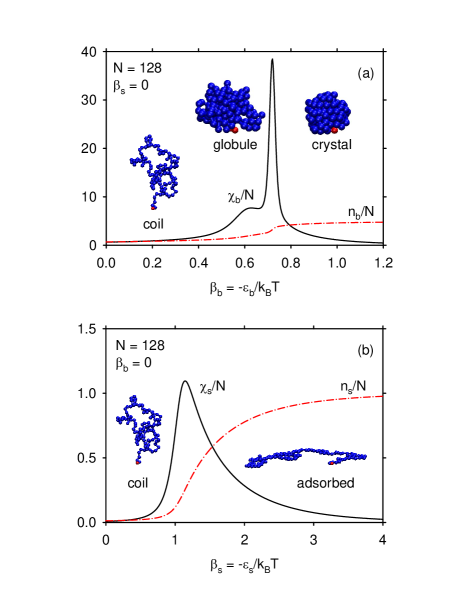
Figure 1: (a) Coil-globule and crystallization transition for chains tethered to a hard surface, $\beta_{s}=0$. The dash-dotted line shows the normalized number of bead contacts, $n_{b}/N$, as a function of solvent quality, $\beta_{b}=-\epsilon_{b}/k_{B}T$, for chain length $N=128$; the solid line represents the normalized bead-contact fluctuations $\chi_{b}/N$. The maxima in $\chi_{b}$ provide estimates for the coil-globule transition, $\beta_{c}\simeq 0.63$, and the freezing transition $\beta_{X}\simeq 0.72$. The insets represent simulation snapshots that illustrate expanded coil, globule, and crystalline chain conformations. (b) Adsorption transition in athermal solvent, $\beta_{b}=0$. The dash-dotted line shows the normalized number of surface contacts, $n_{s}/N$, as a function of $\beta_{s}=-\epsilon_{s}/k_{B}T$ for $N=128$; the solid line represents the normalized surface contact fluctuations $\chi_{s}/N$. The maximum in $\chi_{s}$ provides an estimate for the adsorption transition, which occurs at $\beta_{sa}\simeq 1.14$ for this chain length. The simulation snapshots illustrate expanded coil and adsorbed chain conformations.

The probability to find a chain subject to contact and tension fields in the state $(n_{s},n_{b},z)$ is obtained from

$$P(n_{s},n_{b},z;\beta_{s},\beta_{b},\beta_{f})=\frac{1}{Z}g(n_{s},n_{b},z)\mathrm{e}^{\beta_{s}n_{s}+\beta_{b}n_{b}+\beta_{f}z},$$ (8)

which implies that the density of states needs to be determined only up to a constant prefactor. From the probability distribution we calculate canonical expectation values such as the average height of the last bead

$$\langle z\rangle=\sum_{n_{s},n_{b},z}zP(n_{s},n_{b},z;\beta_{s},\beta_{b},\beta_{f}),$$ (9)

the average number of surface contacts, $\langle n_{s}\rangle$ the average number of bead-bead contacts, $\langle n_{b}\rangle$, as well as fluctuations of these quantities

$$\chi_{s} = \langle n_{s}^{2}\rangle-\langle n_{s}\rangle^{2},$$ (10)

$$\chi_{b} = \langle n_{b}^{2}\rangle-\langle n_{b}\rangle^{2},$$ (11)

$$\chi_{z} = \langle z^{2}\rangle-\langle z\rangle^{2},$$ (12)

$$\chi_{zb} = \langle zn_{b}\rangle-\langle z\rangle\langle n_{b}\rangle,$$ (13)

$$\chi_{t} = \chi_{z}+\chi_{b}+2\chi_{zb}.$$ (14)

In Appendix A we describe the simulation methods we employed to construct the density of state $g(n_{s},n_{b},z)$ over the three-dimensional state space spanned by contact numbers and extensions.

At fixed contact fields $\beta_{s}$ and $\beta_{b}$, the chain extensions, $z$, form a one-dimensional state space with density of states $g(z;\beta_{s},\beta_{b})$, which, after normalization, represents the probability distribution for the extension. The canonical probability distribution

$$p(z;\beta_{s},\beta_{b},\beta_{f})=\frac{1}{Q}g(z;\beta_{s},\beta_{b})\mathrm{e}^{\beta_{f}z},$$ (15)

where $Q=\sum_{z}g(z;\beta_{s},\beta_{b})\mathrm{e}^{\beta_{f}z}$ is the partition function, may be evaluated to find the average extension

$$\langle z\rangle=\sum_{z=0}^{z_{\mathrm{max}}}zp(z;\beta_{s},\beta_{b},\beta_{f})=\left(\frac{\partial\ln Q}{\partial\beta_{f}}\right)_{\beta_{s},\beta_{b}},$$ (16)

and the fluctuations

$$\chi_{z}=\langle z^{2}\rangle-\langle z\rangle^{2}=\left(\frac{\partial\langle z\rangle}{\partial\beta_{f}}\right)_{\beta_{s},\beta_{b}}.$$ (17)

In this statistical ensemble, the tension field $\beta_{f}$ is controlled and the extension $z$ is allowed to fluctuate. This is the approach we take for most of the results presented here. However, when investigating the nature of a transition, it is useful to consider a micro-canonical type of evaluation, where the extension $z$ is controlled and the field $\beta_{f}$ fluctuates. In this formalism, the average tension field $\bar{\beta}_{f}$ at a given height $z$ is calculated from the first derivative of the density of states

$$\bar{\beta}_{f}(z,\beta_{s},\beta_{b})=-\left(\frac{\partial\ln(g)}{\partial z}\right)_{\beta_{s},\beta_{b}},$$ (18)

and the inverse of the fluctuations from the second derivative

$$\chi_{z}^{-1}=\left(\frac{\partial\bar{\beta}_{f}}{\partial z}\right)_{\beta_{s},\beta_{b}}=-\left(\frac{\partial^{2}\ln(g)}{\partial z^{2}}\right)_{\beta_{s},\beta_{b}}.$$ (19)

In Appendix B we describe our Wang-Landau simulations for the 1-d densities of states $g(z;\beta_{b},\beta_{s})$.

When a chain is highly stretched, or when interactions between non-bonded beads are effectively screened, individual bonds respond independently to the applied force. Wittkop et al.Wittkop et al. (1994) enumerated the possible orientations and lengths of the bonds in the BF model to determine a high-tension approximation for the extension of an untethered, athermal chain. To include energetic effects, we note that the beads constituting a bond make a bead-bead contact ($n_{b}=1$) when the bond-length is smaller than $r_{c}=\sqrt{7}$. The number of bond vectors for each pair of $(z_{b},n_{b})$ values defines the single-bond density of states $g_{1}(z_{b},n_{b})$ and is presented in Table 1. For given bead contact and tension fields, the average extension of a single bond is given by

$$\langle z_{b}\rangle=\frac{1}{q_{1}}\sum_{z_{b},n_{b}}z_{b}g_{1}(z_{b},n_{b})\mathrm{e}^{\beta_{f}z_{b}}\mathrm{e}^{\beta_{b}n_{b}},$$ (20)

where $q_{1}=\sum_{z_{b},n_{b}}g_{1}(z_{b},n_{b})\exp{(\beta_{f}z_{b}+\beta_{b}n_{b})}$ is the the single bond partition function. In the independent-bond (IB) approximation, $\langle z_{b}\rangle$ is equal to the normalized extension $z/z_{\mathrm{max}}$, where $z_{\mathrm{max}}=3(N-1)$ is the maximum extension of the chain, and may be compared with simulations results.

Table 1: Single bond density of states; $g_{1}(z_{b},n_{b})$ is the number of single-bond configurations with $z$-coordinate $z_{b}$ and $n_{b}$ contacts between the beads constituting the bond. The total number of bond configurations is 108.

$z_{b}$	0	0	$\pm 1$	$\pm 1$	$\pm 2$	$\pm 2$	$\pm 3$	$\pm 3$
$n_{b}$	0	1	0	1	0	1	0	1
$g_{1}(z_{b},n_{b})$	12	12	8	12	8	9	5	0

III Results

When presenting our results, we measure all interaction energies in units of a positive energy $\epsilon$, temperatures in units of $\epsilon/k_{B}$, and forces in units of $\epsilon/a$, where $k_{B}$ is Boltzmann’s constant and $a$ is the lattice constant. We thus have $\beta_{f}=f/T$, $\beta_{b}=-\epsilon_{b}/T$, and $\beta_{s}=-\epsilon_{s}/T$, where $\epsilon_{b}<0$ and $\epsilon_{s}<0$ for attractive bead-bead and bead-surface interactions, respectively. Unless otherwise stated, we evaluate our density-of-states results in the canonical ensemble, where the fields $\beta_{f}$, $\beta_{b}$, and $\beta_{s}$ are constant and the extension and the contact numbers fluctuate. To ease notation, we omit the angular brackets and write $z$ for $\langle z\rangle$, etc. Similarly, when we perform a microcanonical evaluation of the density of states $g(z,\beta_{s},\beta_{b})$, where the extension $z$ is controlled and the tension field fluctuates, we omit the overbar and write $\beta_{f}$ for $\bar{\beta}_{f}$. We state in the text and in the figure captions when microcanonical evaluations have been performed.

III.1 Force-extension relations for hard surface and athermal solvent conditions

To investigate the mechanical response of a chain to an applied tension force we determine the normalized extension, $z/z_{\mathrm{max}}$, where $z$ is the average height of the last bead, as a function of the tension field $\beta_{f}=f/T$. In Fig. 2 we present force-extension curves for chains of length $N=64$ with hard-core bead-bead interactions, $\beta_{b}=0$, that are tethered either to a hard surface $\beta_{s}=0$, or to a single point (no surface). The inset shows the normalized fluctuations, $\chi_{z}/z_{\mathrm{max}}$, calculated with the aid of Eq. (17). In the absence of a surface, the force-extension curve is antisymmetric with respect to the origin, the magnitude of its slope decreases monotonically with increasing force, and the curve has an inflection point at the origin. In the presence of a hard surface, the extensions are always positive; the average extension is finite when $f=0$, decreases when the chain is pressed against the surface by a negative applied force, and increases when the chain is pulled by a positive force. The force extension curve for the hard surface has an inflection point at a positive applied force value and becomes indistinguishable from the curve for a point-tethered chain soon after.

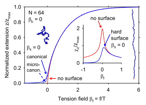
Figure 2: Force-extension relations for chains of length $N=64$ tethered to a hard surface, $\beta_{s}=0$, or to a single point (no surface); both systems are athermal, $\beta_{b}=0$. The solid lines represent results for the normalized extension, $z/z_{\mathrm{max}}$, from the canonical evaluation, Eq. (16), of the densities of states. The dashed line represents the microcanonical result for the force-extension relation of the surface-tethered chain evaluated with Eq. (18). The inset shows the normalized extension fluctuations, $\chi_{z}/z_{\mathrm{max}}$, for chains in the presence and absence of the hard surface. Simulation snapshots of chain conformations at low and high tension force are shown in the left and right part of the figure, respectively.

The fluctuations represent the slope of the force-extension curves, $\chi_{z}=\partial\langle z\rangle/\partial\beta_{f}$, and are the inverse of the (differential) spring constant; the smaller $\chi_{z}$ the more force is required to increase the extension of the chain. A linear regime, corresponding to Hookean springs, requires a constant slope, which is approximately true for a narrow range of near-zero forces (see inset of Fig. 3). In the absence of an applied force, the chain conformations of a free chain have, on average, spherical symmetry while those of a chain tethered to a hard surface are elongated in the direction perpendicular to the surface. This elongation is akin to a pre-stretching of the chain and contributes to the higher spring constant for small forces. Once the chains are sufficiently extended, the effect of the hard surface disappears and the chains show the same response to a further increase in the applied force. Representative chain configurations of unstretched and nearly fully stretched surface tethered chains are included in Fig. 2.

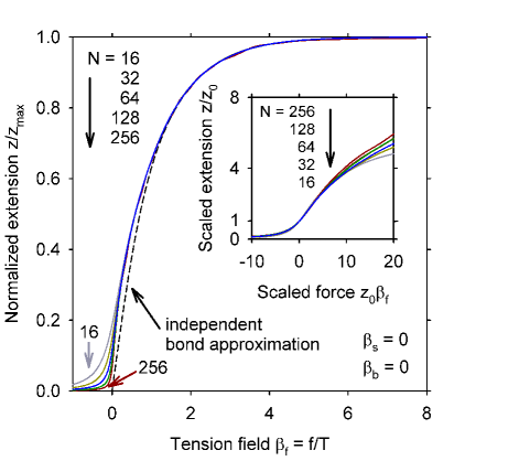
Figure 3: Force-extension relation for contact fields $\beta_{s}=\beta_{b}=0$ and chain lengths $N=16$, 32, 64, 128, and 256. The solid lines represent results for the normalized extension $z/z_{\mathrm{max}}$ from Eq. (16) as a function of the tension field $\beta_{f}$. The dashed line is the independent bond approximation $\langle z_{b}\rangle$ of Eq. (20). The inset shows the scaled extension $z/z_{0}$ as a function of the scaled tension force $z_{0}\beta_{f}$; the data are seen to collapse onto a single curve for small forces.

The force-extension curves represented by solid lines in Fig. 2 have been calculated from a canonical evaluation of the density of states with the aid of Eq. (16). The dashed line shows the microcanonical result for the force-extension relation of the surface-tethered chain calculated with Eq. (18) by taking a numerical derivative (centered-difference approximation without smoothing) of the density of states. The differences between the two evaluation methods are most significant at the lowest forces and extensions. This is not surprising since the canonical and micro-canonical approaches are equivalent in the thermodynamic ($N\rightarrow\infty$) limit and the effects of chain length on the force-extension curves are most significant in the low tension regime, as Fig. 3 shows.

The chain-length dependence of force-extension relations is expected to be different in different force regimes. Figure 3 shows force-extension relations for contact fields $\beta_{s}=\beta_{b}=0$ and different chain lengths. For high and intermediate tension fields, the normalized extension $z/z_{\mathrm{max}}$ is seen to be independent of chain length, in agreement with theoretical predictions that the extension is proportional to the contour length for sufficiently large applied forces. For the highest extensions, the force extension relation is expected to be dominated by the single-bond effects since there are very few interactions between non-bonded monomers. In Fig. 3 we include normalized extensions calculated from the independent-bond (IB) approximation in Eq. (20) with $\beta_{b}=0$. The agreement between simulation and IB results is excellent at the highest tensions, validating our simulation method and showing that interactions between non-bonded beads are not significant for tensions larger than $\beta_{f}\simeq 2$.

As the tension force decreases, the relative extensions $z/z_{\mathrm{max}}$ for different chain lengths start to deviate from each other. Due to the presence of the hard surface, the average height at zero force has a finite value, $z_{0}$, which is expected to scale as $z_{0}\sim N^{\nu}$, where $\nu\simeq 0.6$ is the scaling exponent for good solvent conditions Grosberg and Khokhlov (1994). From Hooke’s law for tethered chains, $z-z_{0}\sim z_{0}^{2}\beta_{f}$, we expect the slope of the force-extension curve at zero force to scale as $N^{2\nu}$. According to Eq. (17), this implies that the height fluctuations scale as $\chi_{z0}\sim N^{2\nu}$ at $\beta_{f}=0$. In Fig. 4 we present results for the height $z_{0}$ and fluctuations $\chi_{z0}$ as a function of chain length, $(N-1)$. The double-logarithmic plot shows good agreement with the scaling predictions given our limited chain lengths. A power-law fit of the $z_{0}$ data for chain lengths larger than 16 yields $\nu=0.62$, while the corresponding fit of $\chi_{z0}$ yields $2\nu=1.21$.

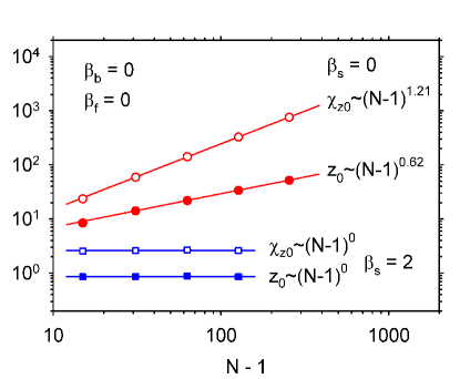
Figure 4: Scaling with chain length of the zero-force extension, $z_{0}$, and fluctuations, $\chi_{z0}$, for hard surface, $\beta_{s}=0$ (circles), and adsorbing surface, $\beta_{s}=2$ (squares), for athermal solvent conditions, $\beta_{b}=0$. The filled and open symbols represent simulation results of $\chi_{z0}$ and $z_{0}$, respectively, for chain lengths $N=16$, 32, 64, 128, and 256 ($\beta_{s}=0$). The solid lines represent power laws with the indicated exponents, for $\beta_{s}=0$ they were obtained from fits to the data for chain lengths $N>16$.

As described in Eq. (4), zero-force extension, $z_{0}$, is the scaling length for low forces. The inset of Fig. 3 shows force extension data in scaled representation, $z/z_{0}$ as a function of $z_{0}\beta_{f}$. While the linear regime where Hooke’s law holds is very small, we find the scaled force-extension graphs to collapse onto a single curve for a sizable range of positive and negative tensions that includes the inflection points of the force-extension curves. Since the fluctuation maxima occur in the low-force scaling region, the peak fluctuations, $\chi_{z}^{*}$, are expected to scale in the same way as the zero-force fluctuations, i.e. $\chi_{z}^{*}\sim z_{0}^{2}\sim N^{2\nu}$. This is confirmed by the chain-length independence of the $\chi_{z}^{*}/z_{0}^{2}$ results for $\beta_{b}=0$ presented in Fig. S1 of the supplementary materialsup . The location of the inflection point scales with the inverse of the zero-force extension, $\beta_{f}^{*}\sim z_{0}^{-1}\sim N^{-\nu}$. Since $\beta_{f}^{*}\rightarrow 0$ as $N\rightarrow\infty$, the effect of the tethering surface disappears in the infinite chain limit as already suggested by the result of Fig. 3.

III.2 Effect of solvent quality

To investigate the effect of solvent quality, we start in the intermediate force regime and apply our model to force-extension experiments on biological molecules (Sec. III.2.1. We then focus on force-induced transitions from compact chain conformations (Sec. III.2.2) before constructing a phase portrait for finite chains in the $\beta_{f}$–$\beta_{b}$ plane (Sec. III.2.3).

III.2.1 Intermediate force regime – Application to biomolecules

Force-extension measurements have become an important tool in investigating conformational properties of polymers. Since many experiments are carried out on chains tethered to non-adsorbing surfaces we set the bead-surface interaction parameter to zero, $\epsilon_{s}=0$. Since we discuss flexible chains in this work, our results apply to molecules such as single-stranded DNA (ss-DNA) but not to the very stiff double-stranded DNA (ds-DNA) or the PEG chains investigated by Dittmore et al.Dittmore et al. (2011).

Saleh et al.Saleh et al. (2009) investigated the scaling behavior of single chains under tension by measuring force-extension curves of denatured single-stranded DNA molecules in solvents of different salt concentrations, spanning the range from good to poor solvent conditions. For intermediate tensions, Saleh et al.Saleh et al. (2009) observed power law behavior for the extension as a function of tension, $R_{z}\sim f^{\gamma}$, with exponents $\gamma$ near the predicted value $\gamma=2/3$ for good to moderate solvent conditions (see Eq. (3)). For very good solvents, the experiments yielded somewhat smaller exponents, $\gamma\simeq 0.6$, while the transition to poor solvent conditions resulted in a large increase of the exponents.

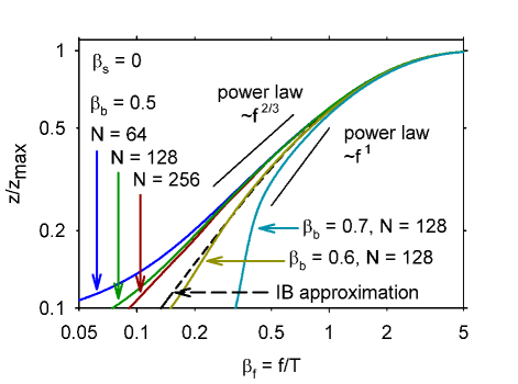
Figure 5: Normalized extension $z/z_{\mathrm{max}}$ as a function of tension field $\beta_{f}$ for a hard surface ($\epsilon_{s}=0$) and three different solvent conditions. The solid lines represent simulation results for chains of length $N=64$, 128, and 256 for $\beta_{b}=0.5$, and $N=128$ for $\beta_{b}=0.6$, and $\beta_{b}=0.7$ as indicated in the figure. The dashed line represents the independent bond (IB) approximation, Eq. (20), for $\beta_{b}=0.6$, which is barely distinguishable on this scale from IB results for $\beta_{b}=0.5$ and $\beta_{b}=0.7$. Line segments of slope $2/3$ and 1 illustrate predicted power laws.

To explore the elastic response of chains in moderate and poor solvents, we determined force-extension curves for three values of the bead-contact field $\beta_{b}$ near the coil-globule transition ($\beta_{c}=0.63$) of a chain of length $N=128$. In Fig. 5 we present these results in a log-log plot to facilitate comparison with Fig. 1(a) of Ref. [Saleh et al., 2009]. The inset of Fig. 6 also includes good-solvent data in log-log representation. In qualitative agreement with experimental data Dessinges et al. (2002); Saleh et al. (2009) we find that the effect of solvent quality increases with decreasing tension force. For high tensions the independent bond (IB) approximation of Eq. (20), indicated by the dashed line, describes the simulation data well. As the tension decreases, interactions between different chain segments become important and the IB approximation begins to fail. For $\beta_{b}=0.5$, excluded volume interactions expand the chain and the IB approximation underestimates the extension. Ideal (IB) behavior is observed over the largest force range for $\beta_{b}=0.6$, where the chain is closest to the coil-globule transition and excluded volume interactions are expected to be screened by attractive interactions. The IB curve varies nearly linearly with force for the lower tension range shown in this graph. For poor solvent condition, $\beta_{b}$ = 0.7, the actual extension is smaller than in the IB approximation since the strongly attractive interactions between chain segments favor compact configurations. The steep part of the force-extension curve for $\beta_{b}=0.7$ belongs to a force-induced transition from the globule to the extended chain conformations (see Sec. III.2.2). This is followed at higher tension by the stretching of an extended chain in poor solvent. In this regime, scaling arguments predict a linear dependence of the extension on the force Halperin and Zhulina (1991a). A comparison with a line segment of unit slope in Fig. 5 shows approximately linear behavior of our results in a narrow force range following the transition.

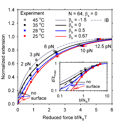
Figure 6: Normalized extension as a function of reduced force $bf/k_{B}T$ in linear scale (main figure) and log-scale (inset). The symbols represent experimental data on ssDNA by Danilowicz et al.Danilowicz et al. (2007) at temperatures 25 ⁰C, 28 ⁰C, 35 ⁰C, and 45 ⁰C and forces between 2 and 12.5 pN. The solid lines represent our results for $N=64$ at contact fields $\beta_{b}=-1.5$, 0, 0.5, and 0.67. The force extension curves for $\beta_{b}=0$ and 0.5, and 0.67 are calculated from dedicated (1-d) simulations at these contact fields; for $\beta_{b}=-1.5$, the force-extension curve evaluated from the 3-d density of states is supplemented at high tension with results from the independent bond (IB) approximation. The segment lengths are $b=1.73$ nm and $b=1.7$ lattice constants for experimental and simulation data, respectively. The dash-dotted lines represent results for point-tethered chains (no surface). Note that graph for $\beta_{b}=0.67$ has an inflection point near $b\beta_{f}=0.54$.

To illustrate the power law prediction of Eq. (3) at intermediate tensions, we have included a straight line segment of slope 2/3 in Fig. 5. An inspection of our results in Fig. 5 shows that the calculated curves straighten for intermediate tensions but never quite lose their curvature. While much larger chain lengths are required to observe power law behavior Hsu and Binder (2012), our results for different solvent conditions in Fig. 5 and the inset of Fig. 6 exhibit important properties of the intermediate force regime. A comparison of results for chain lengths $N=64$, 128, and 256 at $\beta_{b}=0.5$ in Fig. 5 shows that the chain length dependence of the normalized extension is most pronounced at low tensions and disappears as the tension increases. This agrees with our observations on chains in athermal ($\beta_{b}=0$) solvents and is related to the low-force scaling behavior of the extension. To illustrate the effect of the hard tethering surface, we include results for point-tethered chains (no surface) in the inset of Fig. 6. They show that the effect of the tethering surface decreases rapidly with increasing tension even for relatively short chains. Hence, in the intermediate force regime, neither the chain length nor the presence of the tethering surface affect the relative extension of the chain. In this regime, the solvent quality determines the mechanical response of the chain with a decrease in solvent quality leading to a steeper increase of the extension.

The universal nature of force-extension relations in the intermediate force regime encourages us to compare our simple, implicit solvent model with experimental data on a complex biomolecule. Danilowicz and coworkers Danilowicz et al. (2007) investigated the effect of temperature on the force-extension relation of single-stranded DNA ($\lambda$-phage ssDNA) in phosphate buffer saline solution by performing magnetic tweezer experiments at several temperatures between 25 ⁰C and 50 ⁰C. At the lower temperatures, base pairing leads to the formation of hairpins, which reduce the size of the coil. As the temperature increases, the number of hairpins decreases and the coil swells until a temperature of about 40⁰C, where no more hairpins are formed and the chain dimensions are comparable to chemically denatured single-stranded DNA (dssDNA). To compare simulation results for our model with experimental data we select four isotherms, 25 ⁰C, 28 ⁰C, 35 ⁰C, and 45 ⁰C, from the data presented in Fig. 3 of Danilowicz et al.Danilowicz et al. (2007). We reduce the measured extension $x$ by the contour length $L$, $\hat{z}=x/L$, and calculate the dimensionless force $bf/k_{B}T$, where $b$ is a Kuhn segment length and $k_{B}$ is Boltzmann’s constant. Values of $L=23.5$ $\mu$m and $b=1.73$ nm are obtained from a description of experimental data at 25 ⁰C in terms of an extensible freely-jointed chain model Smith et al. (1996), which also yields $S=300$ pN for the stretch modulus Danilowicz et al. (2007). From our simulation data for chain length $N=64$, we calculate force-extension curves for several values of the bead-contact field $\beta_{b}$ corresponding to a range of solvent conditions. For this chain length, the collapse transition occurs at about $\beta_{c}=0.69$ and we choose $\beta_{b}=0.67$ as our highest contact field (poorest solvent condition). To convert the tension field $\beta_{f}$ to the reduced force $b\beta_{f}$, we consider the chain dimensions at $\beta_{b}=0.67$ and estimate an effective segment length of $b=1.7$ from $b=R_{e}^{2}/(N-1)b_{l}$, where $b_{l}$ is the average bond length. As before, we reduce the extension $z$ by the maximum extension $z_{\mathrm{max}}=3(N-1)$. In Fig. 6 we present experimental and simulation force-extension data at four temperatures and $\beta_{b}$ values, which were chosen to approximate the experimental data at 2 and 3 pN. The inset shows the data in log-log presentation for easier comparison with Fig. 5. Three of the curves in Fig. 6 represent results from Wang-Landau simulations at fixed fields $\beta_{s}=0$ and $\beta_{b}=0.67$, $\beta_{b}=0.5$, and $\beta_{b}=0$, respectively. The result for $\beta_{b}=-1.5$, was calculated from the 3-d density of states $g(n_{s},n_{b},z)$, which is reliable in a limited range of tensions. At the highest tensions we therefore supplement the data with results from the independent bond approximation.

Fig. 6 shows that our model is able to describe experimental data for moderately high forces. The behavior of the biomolecule at the highest forces is not captured by our model. In this regime, the bonds of ssDNA molecules become extensibleSmith et al. (1996), while the bond-fluctuation model has a limited bond length. The lowest extensions in Fig. 6 correspond to the lowest temperature, 25 ⁰C and highest $\beta_{b}$ value, $\beta_{b}=0.67$. The relatively steep decline at low force shows the proximity to the collapsed state and indicates that many bead-bead contacts are formed, approximating the formation of hairpins in the ssDNA. Since $\beta_{b}=-\epsilon_{b}/k_{B}T$ and $\epsilon_{b}<0$ for net attractive interactions, a decrease in $\beta_{b}$ corresponds to an increase in temperature. The next isotherm in the physical system is at 28 ⁰C, only about 1% above the first in absolute temperature. The corresponding isotherm in the model, on the other hand, is at $\beta_{b}=0.5$, about 25% from the first. Part of the reason for the larger change in the model temperature is the size of the chain. The shorter a chain, the larger the transition region near the collapse transition, which implies that the biological molecule requires a much smaller change in temperature for an equivalent change in solvent conditions. Taking this finite-size effect into account is not sufficient to reach the highest isotherms; for the 35 ⁰C degree isotherm, for example, athermal contact conditions ($\beta_{b}=0$) in the model barely match the experimental data, while net repulsive bead-bead interactions $\beta_{b}<0$ are required to reach even larger extensions. The biological molecule is a polyelectrolyte in a complex aqueous solvent mixture Cocco et al. (2003) where changes in temperature affect, for example, ion concentration and hydrogen bonding rates, so that the net segment-segment interactions vary with temperature. At the highest temperature, 45 ⁰C, where the molecule is denatured, the solvent-segment interactions are much more attractive than the segment-segment interactions leading to a swelling of the coil. In an implicit solvent model, such as the bond-fluctuation model employed in this work, solvent-solvent, bead-bead, and bead-solvent interactions are described by a single, net interaction parameter $\epsilon_{b}$, which has to be adjusted if a complex solvent system is to be described in a temperature range where the solvent quality changes rapidly.

III.2.2 Force-induced transitions from globular and crystalline states

For a collapsed polymer chain under tension, Halperin and ZhulinaHalperin and Zhulina (1991a) predicted that the force induces a discontinuous transition between a deformed globule at low tension and a stretched chain at high tension. At the transition force, which we call $f^{*}$, coexistence between states leads to a plateau in the force as a function of extension (or a vertical jump in the extension as a function of force). A number of simulation studies (see e.g. Refs. [Wittkop et al., 1996; Grassberger and Hsu, 2002; Frisch and Verga, 2002]) have confirmed the first-order nature of the transition and identified chain conformations with globular and string-like sections on the same molecule in the transition region. More recently, Walker and coworkers Gunari et al. (2007); Li and Walker (2010) performed single-chain pulling experiments on poly(styrene) (PS) in water, a poor solvent, and a range of solvents of different quality. The measured force-extension curves of PS in water Gunari et al. (2007) show clearly a plateau in the force and confirmed experimentally the theoretical prediction of a first-order transition. A careful study of the transition force $f^{*}$ for PS in a range of solvent mixtures shows a linear dependence of $f^{*}$ on the interfacial energy between the polymer and the solvent.Li and Walker (2010)

In Fig. 7 we present stretching results for chains of length $N=128$ in four solvent conditions ranging from athermal to poor. Panels (a) and (c) show force-extension curves in linear scale for a large and a restricted range of extensions, respectively. Panel (b) shows graphs of the normalized fluctuations $\chi_{z}/z_{\mathrm{max}}$ which, according to Eq. (17) represent the slopes of the force-extension curves in (a). The fluctuation maxima indicate the inflection points in the force-extension curves. With increasing $\beta_{b}$, the location of the maximum, which we call $\beta_{f}^{*}$, moves to higher tensions while the height of the peak, $\chi_{z}^{*}/z_{\mathrm{max}}$, first decreases and then increases as the solvent quality becomes poorer.

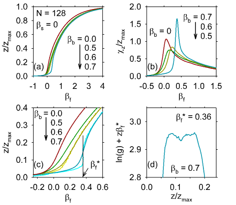
Figure 7: Chain stretching in good and poor solvent. (a) Force-extension curves, in linear scale, for chains of length $N=128$ tethered to a hard surface $\beta_{s}=0$. The bead contact fields represent athermal, $\beta_{b}=0$, moderate, $\beta_{b}=0.5$, near $\theta$, $\beta_{b}=0.6$, and poor solvent, $\beta_{b}=0.7$, conditions respectively. (b) The normalized fluctuations of the extension $\chi_{z}/z_{\mathrm{max}}$, are equal to the slopes of the force extension curves in (a). (c) Transition region of the force-extension curves in (a). The bright (somewhat noisy) lines represent results from a microcanonical evaluation of the densities of state for $\beta_{b}=0.6$ and 0.7. The vertical line segment indicates the tension field at the transition, $\beta_{f}^{*}$, and highlights the vertical part of the microcanonical extension curve. (d) Evidence for a bimodal probability distribution for the tension field $\beta_{f}^{*}=0.36$ at $\beta_{b}=0.7$; the solid line shows the reweighted density of states, $\ln(g)+z\beta_{f}^{*}$ as a function of normalized extension, $z/z_{\mathrm{max}}$.

For the poor-solvent case, $\beta_{b}=0.7$, our results agree with the predictions of Halperin and ZhulinaHalperin and Zhulina (1991a): The force-extension curve in panel (c) shows an extended linear region at low tension corresponding to the deformation of the globule, followed by a steep increase as the chain transitions from globule to extended conformations. Beyond the transition, the extended chain is stretched further and differences between chains in different solvents gradually diminish. For $\beta_{b}=0.7$, the extension fluctuations in panel (b) show a tall and narrow peak at $\beta_{f}^{*}\simeq 0.37$, which is consistent with a discontinuous transition of a finite chain. To investigate the transition further, we include results from a microcanonical evaluation of $g(z;\beta_{s},\beta_{b})$ for $\beta_{b}=0.6$ and $\beta_{b}=0.7$ in panel (c) (bright lines). For finite chain lengths, canonical and microcanonical results are not identical. In the canonical evaluation of $g(z;\beta_{s},\beta_{b})$ with Eq. (16), the summation over all states (weighted by the appropriate Boltzmann factors) leads to a smoothing of calculated extensions, which may obscure localized features, such as the vertical rise in extension expected near a discontinuous transition. In the microcanonical evaluation with Eq. (18), the numerical derivative of $g$ that yields $\beta_{f}(z)$ involves only the two neighboring values of $g$ at $z\pm 1$; the results are therefore highly local but also somewhat noisy. For $\beta_{b}=0.6$, neither evaluation method suggests a discontinuous transition. For $\beta_{b}=0.7$, however, the microcanonical force extension curve shows a nearly vertical rise at $\beta_{f}^{*}=0.36$, suggesting a discontinuous transition. For a finite-size system, a first-order transition is accompanied by changes in curvature of the density of states, which we describe in more detail below. For the microcanonical force extension curve, this leads to an “S”-shaped rather than vertical line in the coexistence region, which is barely visible through the noise in the force-extension curve presented in panel (c). The coexistence of states at the transition field is reflected in the probability distribution for the extensions, which according to Eq. (15), is given by $\ln(p)=\ln(g)+z\beta_{f}^{*}-Q$, where $Q$ is the normalization constant. The results for $\ln(g)+z\beta_{f}^{*}$ presented in panel (d) show the bimodal nature of the probability distribution a the transition field $\beta_{f}^{*}$.

The first order nature of the transition becomes more pronounced as the solvent condition worsens and the chains crystallize. We would like to stress that the crystal structures found in our model reflect the symmetry of the underlying simple cubic lattice and have nothing to do with the crystal structure of biological and synthetic polymersLuettmer-Strathmann et al. (2008). Similarly, the transition to the crystalline state in our model involves the spatial rearrangement of flexible chain segments and is quite different from the crystallization transition observed in synthetic polymers, where sections of the chain stiffen and fold back on themselves to form crystallites. In Fig. 8 we show results for a chain of length $N=32$ that is pulled out of the crystalline phase. The density of states for $\beta_{b}=2$ presented in panel (a) and its inset has two characteristic features. First, the values of $\ln(g)$ show discrete jumps up and down at low extensions due to the crystalline order of the chain. Second, the curvature of the $\ln(g)$ graph changes from concave to convex and back again as the extension increases. As is well known, such a “convex intruder” indicates the presence of a discontinuous transition in a finite-size system. Upon reweighting with the transition field $\beta_{f}^{*}=2.6$ we obtain the bimodal probability distribution shown in panel (b). Note that the maximum in the probability distribution at low extension shows the discrete jumps characteristic for crystalline states. Panel (c) shows extensions $z/z_{\mathrm{max}}$ and fluctuations $\chi_{z}$ as a function of the tension field $\beta_{f}$. The fluctuations are very small in the crystalline state and have a tall and narrow peak at the transition field. At the lower extensions, the response to the applied force is almost entirely due to reorientation of the crystal without significant loss of bead-bead contacts (of all the available crystalline chain conformations, those that are oriented with their long axis perpendicular to the surface become increasingly probable with increasing tension force). Since the bead-bead interactions are highly attractive, high tensions field, larger than about $\beta_{f}=2.0$, are required to induce conformational changes (defects) that lead to a break-up of the compact crystal at the transition field $\beta_{f}^{*}=2.6$. The transition states are chain conformations with stretched chain segments attached to compact crystallites; an example is shown in Fig. 8. The force-extension curve beyond the stretching transition is well described by the independent bond approximation, shown as a dashed line at high tension, indicating that essentially all contacts between non-bonded beads are lost in the stretching transition.

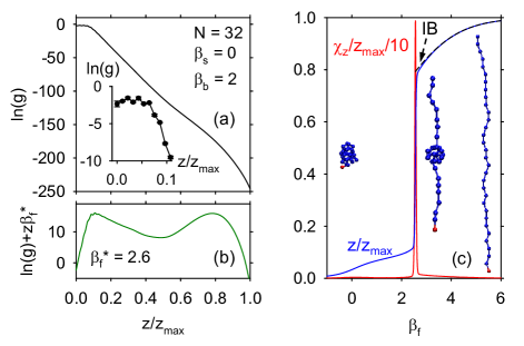
Figure 8: Chain stretching from the crystalline state. (a) Logarithmic density of states $\ln(g(z))$ as a function of the normalized extension $z/z_{\mathrm{max}}$ (solid line) for a chain of length $N=32$ with crystalline order, $\beta_{b}=2.0$. The inset shows the low extension region, where the crystalline order leads to discrete jumps in the density of states; the symbols connected by lines represent the $\ln(g(z))$ values. (b) Logarithmic density of states reweighted with the transition tension $\beta_{f}^{*}=2.6$. (c) Normalized extension $z/z_{\mathrm{max}}$ and fluctuations $\chi_{z}$ as a function of the tension field $\beta_{f}$. The blue solid line represents $z/z_{\mathrm{max}}$ values obtained from a canonical evaluation of the density of states; the dashed line at high tension shows the independent bond (IB) approximation for $\beta_{b}=2$. The red solid line shows fluctuation values that have been divided by $10z_{\mathrm{max}}$ to fit into the figure; the fluctuation have a tall and very narrow peak at the transition field $\beta_{f}^{*}$. The simulation snapshots show chain conformations corresponding to the crystalline state before the transition (left), a transition state with coexisting crystallite and stretched chain segments (center), and a stretched chain (right).

III.2.3 Phase portrait for finite chains in solvent

To provide a comprehensive description of the effect of solvent quality on chain stretching and the effects of tension on chain collapse we construct a phase portrait in the $\beta_{f}$–$\beta_{b}$ plane for chains of length $N=64$ tethered to a hard surface, $\beta_{s}=0$. In Fig. 9 we show locations of fluctuation maxima separating regions of different conformations of the chain. In the absence of tension, the good solvent region at small $\beta_{b}$ is separated from the poor solvent region at high $\beta_{b}$ by a region where the solvent is near $\theta$ conditions. The $\theta$ point for free chains of this model, estimated by extrapolating coil-globule transition temperatures to infinite chain lengths, is about $\beta_{\theta}=0.46$ Rampf et al. (2005). The finite chains considered here enter a $\theta$ region around $\beta_{b}=0.5$; we find, for example, that the chain dimensions of surface tethered chains scale approximately as $N^{1/2}$ at $\beta_{b}=0.5$. The $\theta$-region ends with the collapse transition, which occurs at $\beta_{c}=0.69$ for $N=64$.

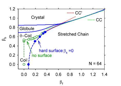
Figure 9: Phase portrait for tethered chains of length $N=64$ in the space of tension field, $\beta_{f}$, and bead-contact field, $\beta_{b}$. Crystal and globule are ordered phases at high bead-contact fields, i.e. in poor solvent. In the disordered phase we indicate regions of stretched, $\theta$-coil, and expanded coil conformations. The solid and dashed blue lines show the location of fluctuation maxima determined from an evaluation of the 3-d density of states $g(n_{s},n_{b},z)$ for chains tethered to a hard surface, $\beta_{s}=0$. The dashed line show the location of inflection points of the force extension curves at low $\beta_{b}$, which are not associated with a phase transition. The filled symbols represent the location of inflection points ($\chi_{z}$ maxima) obtained from 1-d Wang-Landau simulations at fixed $\beta_{b}$ and $\beta_{s}=0$. The open symbols connected by green lines show inflection point locations from simulations in the absence of a hard surface. The dotted lines labeled CC and CC’ are straight lines with slopes of 0.41 and 0.62, respectively, estimated from generalized Clausius-Clapeyron relations.

Good and $\theta$ solvent, $\mathbf{\beta_{b}\lesssim 0.69}$

The dashed blue line and filled symbols in Fig. 9 indicate $\chi_{z}$ maxima for chains tethered to a hard surface obtained from an evaluation of the density of states $g(n_{s},n_{b},z)$ and from 1-d Wang-Landau simulations, respectively. The dashed green line and open symbols show the corresponding results in the absence of the hard surface. As discussed in Sec. III.1, the inflection points occur at zero force for free (no surface) chains and at positive forces for surface-tethered chains. They are shown as dashed lines in the diagram since they do not represent phase transitions, even in the infinite chain limit.

It is interesting to compare free and surface tethered chains under tension as the solvent quality decreases. For small increases in $\beta_{b}$, the inflection points of the free chains remain at $\beta_{f}=0$, while those for tethered chains move to slightly higher tension fields $\beta_{f}$. With increasing $\beta_{b}$, the peak heights $\chi_{z}^{*}$ for tethered chains decrease until they reach a minimum when the chains enter the $\theta$-solvent region (this is seen in Fig. 7 for $N=128$); for chain length $N=64$, the minimum occurs at $\beta_{b}=0.53$. At $\beta_{b}=0.53$, the fluctuations $\chi_{z}(\beta_{f})$ of free chains show a very broad maximum at $\beta_{f}=0$, which splits into a minimum at $\beta_{f}=0$ and two symmetric maxima at finite $\beta_{f}$ values as $\beta_{b}$ increases further. The inflection point corresponding to the positive tension maximum is just visible in the point-tethered force-extension curve for $\beta_{b}=0.67$ included in Fig. 6. In Fig. 9 we show the positive branch of peak locations for free chains. As the solvent conditions change from $\theta$ solvent to poor solvent, the peak locations of the free chains approach those of the tethered chains.

The scaling with chain length of the scaled fluctuation maxima, $\chi_{z}^{*}/z_{0}^{2}$, where $z_{0}$ is the zero-force extension, depends on the solvent conditions and is discussed in the supplemental materialssup . The results presented in Fig. S1 suggest that chain stretching acquires the character of a phase transition as the solvent quality decreases. The transition from $\theta$–region coils to stretched chains appears to be continuous. After a small initial deformation of the coil at low forces, the extension and number of bead contacts change rapidly through the transition region, before the extended chain is stretched further at higher forces. Since the $\theta$–region decreases in size with increasing chain length this kind of transition is not expected to exist in the limit of infinite chain length.

Poor solvent – coil-globule and freezing transition under tension

In poor solvent conditions, we find two types of compact states: the globule, a high-density, amorphous state and the crystal, characterized by order of the chain segmentsLuettmer-Strathmann et al. (2008). To construct the lines in the phase portrait separating the regions of coil, globule, and crystal conformations we consider chains under fixed tension field as the solvent quality changes. In Fig. 10 we present results for the fluctuations in the number of bead contacts $\chi_{b}$ as a function of $\beta_{b}$ at constant tension field $\beta_{f}=f/T$ for chains of length $N=64$. The inset of Fig. 10 shows normalized extensions values, $z/z_{\mathrm{max}}$, in the transition region. In the absence of tension (black solid line), the fluctuations show two peaks, one at $\beta_{c}=0.69$ indicating the coil-globule transition and another at $\beta_{X}=0.85$ corresponding to the crystallization transition. When a tension field of $\beta_{f}=0.3$ is applied, the coil-globule peak moves to a higher $\beta_{b}$ value and sharpens, while the tension has little effect on the crystallization transition. The graphs in the inset show a strong decrease of the extension during the coil-globule transition while only small changes in height are associated with the crystallization transition. As the tension increases further, the coil-globule transition peak continues to move closer to the crystallization peak until the peaks overlap completely; from then on a single peak continues to grow in height and move slowly to higher $\beta_{b}$ values. At the highest tension, the transition is between a highly stretched strand and a crystalline phase, as we saw in the example for $N=32$. For intermediate tensions, around $\beta_{f}=0.5$, collapse and crystallization are distinct even though the contact fluctuations show one broad maximum. A good estimate for the crystallization transition may be obtained from the combined fluctuations $\chi_{t}$, defined in Eq. (14), and shown as a dashed line for $\beta_{f}=0.5$ in Fig. 10. The quantity $\chi_{t}$ represents fluctuations of the sum $(z+n_{b})$. Near the coil-globule transition, the extension decreases rapidly as the number of bead contact grows (see inset of Fig. 10). This makes $\chi_{t}$ smaller than $\chi_{b}$ and more sensitive to fluctuations due to local rearrangements of chain segments, which characterize the crystallization transition. In the phase portrait, Fig. 9, we show as solid blue lines locations of $\chi_{b}$ maxima separating coil and globule regions and $\chi_{t}$ maxima separating globule and crystal regions. Fig. 9 shows a narrow $\theta$–coil region between the globule and stretched chain regions, which is a finite-size effect. The lines bordering this region represent maxima of different fluctuations: bead-contact fluctuations for the boundary of the globule region and extension fluctuations for the stretched chain region. For finite systems, it is not uncommon that different quantities show transitions at somewhat different fields and that the differences decrease with system size. Ferrenberg and Landau (1991) We find for our model, too, that the size of the intervening region decreases markedly from $N=32$ over $N=64$ to $N=128$.

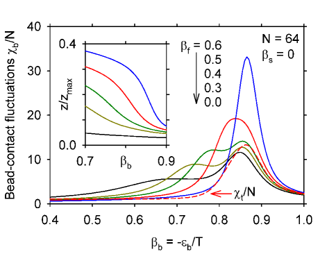
Figure 10: Chain collapse under tension. The solid lines represent normalized fluctuations in the number of bead-contacts, $\chi_{b}/N$, as a function of bead-contact field, $\beta_{b}$, for applied tension fields $\beta_{f}=0.6$, 0.5, 0.4, 0.3, and 0.0. The dashed red line represents the combined fluctuations, $\chi_{t}$ defined in Eq. (14), for $\beta_{f}=0.5$. The inset shows the corresponding normalized extension $z/z_{\mathrm{max}}$ in the range of $\beta_{b}$ values, where the tension has the largest effect on the collapse transition.

Poor solvent – transitions to stretched chain conformations

In the infinite chain limit, transitions from crystalline to amorphous states are always discontinuous. For the chains of length $N=64$ considered in Fig. 9, we observe two-phase coexistence, characteristic of first-order transitions, between crystal and globule and between crystal and stretched chains.

The line separating crystal and stretched chains increases nearly linearly with increasing $\beta_{f}$ in the tension range considered here. For first-order transitions, the slope of the transition line in a diagram of field variables may be estimated from a Clausius-Clapeyron (CC) type equation. For chains tethered to a hard surface it takes the form $d\beta_{b}/d\beta_{f}=-\Delta z/\Delta n_{b}$, where $\Delta z$ and $\Delta n_{b}$ are the differences in extension and number of bead contacts of the coexisting states, respectively. Simulation results for crystalline and stretched states for $N=64$, $\beta_{f}=1.0$, $\beta_{b}\simeq 1.0$ yield a slope of 0.41 for the coexistence line at $\beta_{f}=1.0$. A straight line segment of slope 0.41 is superimposed as a dotted green line on the coexistence curve in Fig. 9 and seen to describe the transition line well up to almost the highest tension fields in the figure. For higher tensions, the slope of the coexistence curve increases gradually. In the limit as both $\beta_{b}\rightarrow\infty$ and $\beta_{f}\rightarrow\infty$, the coexisting states are a stretched chain of independent bonds and a crystal that has the maximum number of contacts for the given chain length. For $N=64$, $n_{b,\mathrm{max}}/N=4.5$, predicting a limiting value of 0.57 for the slope. For $N\rightarrow\infty$, the crystal structure yields $n_{b,\mathrm{max}}/N=6$ and a limiting slope of 0.4. In general, the CC analysis predicts a decreasing slope of the crystal-stretched chain coexistence curve with increasing $N$, which we observe for the chain lengths considered in this work. For $N=32$, where we also have 1-d Wang-Landau results for crystalline chains, we find good agreement between the high-field CC prediction and the slope of the coexistence curve.

The line of first-order transitions separating crystalline and globular states in Fig. 9 is almost independent of the applied tension field. In contrast, the coil-globule transition occurs at increasing $\beta_{b}$ values as $\beta_{f}$ increases, thus reducing the $\beta_{b}$ range of the globule until the globular phase disappears at high tension. For long chains, the force-induced transition is discontinuous with two-state coexistence, as we have seen, for example, in Fig. 7 for $N=128$ at $\beta_{b}=0.7$. For shorter chains and at $\beta_{b}$–values closer to the coil-globule transition, the fluctuations in the system are too large for phase coexistence to occur and the stretching transition becomes continuous. In this case, we may estimate the slope of the transition line from a modified Clausius-Clapeyron equation, which reads $d\beta_{b}/d\beta_{f}=-\chi_{z}/\chi_{zb}$. Evaluating $\chi_{z}$ and $\chi_{zb}$ for $N=64$ at $\beta_{f}=0.53$ and $\beta_{b}=0.81$, we find a slope value of 0.62. The line-segment of slope 0.62 included in Fig. 9 is a good approximation to the stretching transition line in the globule-range of $\beta_{b}$ values. A linear relationship between $\beta_{f}$ and $\beta_{b}$ at the stretching transition is consistent with the experimental observation by Li et al.Li and Walker (2010) that the force plateau depends linearly on the interfacial energy between polymer and solvent.

III.3 Effect of surface attraction

The presence of an attractive surface affects the mechanical response of a tethered chain to a force perpendicular to the surface. To study the effects of surface attraction on force-extension relations and to investigate the effect of tension on the adsorption transition, we focus on athermal solvent conditions and keep the bead-contact field at zero, $\beta_{b}=0$. An analysis of the density of states shows that the adsorption transition, identified from a maximum in $\chi_{s}$ (Eq. 10), occurs near $\beta_{sa}=1.18$ for $N=64$ and $\beta_{sa}=1.14$ for $N=128$ (see Fig. 1 (b)); as $N\rightarrow\infty$, $\beta_{sa}\rightarrow 0.98\pm 0.03$Descas et al. (2004); Decas et al. (2008). For $\beta_{s}<0.8$, we find the force extension relations to be very similar to the hard surface case (see Fig. 3). We thus refer to surface contact fields with $\beta_{s}<0.8$ as slightly attractive and investigate larger $\beta_{s}$ values in detail.

In Fig. 11 (a) we present force-extension curves for chains of length $N=64$ tethered to surfaces with several surface contact fields from $\beta_{s}=0$ (hard surface see Sec. III.1) to $\beta_{s}=2.0$; Fig. 11 (b) shows the normalized number of surface contacts, $n_{s}/N$, as the chains are being pulled. At high tension fields, the chains are stretched away from the surface; $n_{s}/N$ approaches $1/N$ and the extensions become independent of the surface interactions as $\beta_{f}$ becomes very large. For low forces, that is for $\beta_{f}$ values that are too small to change the number of surface contacts significantly, the adsorbed chains ($\beta_{s}=1.5$ and $\beta_{s}=2.0$ in Fig. 11) have much lower extensions and much higher (differential) spring constants than the desorbed chains. This is expected because, for adsorbed chains, a small applied force changes only the conformation of the unadsorbed tail of the chain. Since the length of the tail decreases with increasing $\beta_{s}$ and vanishes as $\beta_{s}$ becomes very large (strong coupling limit), both zero-force extension and fluctuations decrease with increasing $\beta_{s}$. Fig. 4 includes data for the zero-force extension, $z_{0}$, and inverse spring constant, $\chi_{z0}$, at $\beta_{s}=2$ for a range of chain lengths from $N=16$ to $N=128$. The results show that $z_{0}$ and $\chi_{z0}$ are independent of $N$, consistent with the length of the desorbed tail being independent of the chain length.Eisenriegler et al. (1982); Decas et al. (2008)

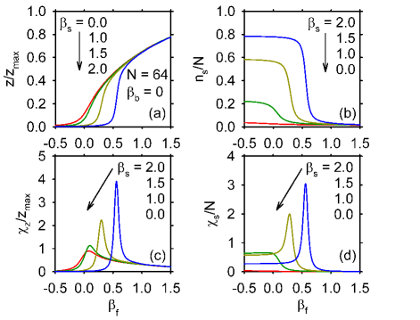
Figure 11: Effect of surface attraction on tethered chains under tension for chain length $N=64$ in athermal solvent conditions, $\beta_{b}=0$. (a) Normalized extension $z/z_{\mathrm{max}}$ as a function of tension field, $\beta_{f}$, for surfaces with increasingly attractive interactions, $\beta_{s}=0$, 1.0, 1.5, and 2.0. (b) Normalized surface contacts $n_{s}/N$, (c) normalized extension fluctuations $\chi_{z}/z_{\mathrm{max}}$, and (d) normalized surface-contact fluctuations $\chi_{s}/N$ as a function of $\beta_{f}$ for the same surface-contact fields $\beta_{s}$.

For adsorbed chains, an increase in the tension field is expected to lead to force-induced desorption. The graphs for $\beta_{s}=1.5$ and $\beta_{s}=2.0$ in Fig. 11 (a) and (b) show a sharp increase in extension and a simultaneous loss of surface contacts within a narrow force range. Increase in chain extension and loss of surface contacts are more gradual for $\beta_{s}=1.0$, where the chains are desorbed but close to the adsorption transition. For chains tethered to hard surfaces, $\beta_{s}=0.0$, the number of surface contacts is already small at zero force. In Fig. 11 (c) and (d), we present extension fluctuations, $\chi_{z}$, and surface contact fluctuations, $\chi_{s}$, respectively, corresponding to the force-extension curves in panel (a). For all surface conditions, the extension fluctuation graphs in panel (c) show a maximum. These peaks move to higher tension fields and become sharper as $\beta_{s}$ increases. The surface-contact fluctuations shown in panel (d), on the other hand, have well defined peaks only for adsorbing surfaces. For hard surfaces, $\chi_{s}$ decreases monotonically as $\beta_{f}$ increases. As $\beta_{s}$ approaches the adsorption value, the graph of $\chi_{s}$ develops first a plateau at low $\beta_{f}$ and then a maximum. The $\chi_{s}$ graph for $\beta_{s}=1.0$ in Fig. 11 (d) is right on the verge of having a maximum, consistent with $\beta_{sa}\simeq 1.0$. A comparison of the $\chi_{z}$ and $\chi_{s}$ graphs for $\beta_{s}=1.5$ and $\beta_{s}=2.0$ shows similar behavior for both types of fluctuations in the transition region. With increasing surface attraction, the peak heights grow and the peaks occur at higher fields. The peaks in the extension fluctuation and the surface-contact fluctuations occur at somewhat different tension fields; the difference between the peak locations decreases rapidly as the surface attraction increases and it also decreases with increasing chain length. The gap between the transition fields determined from peaks in $\chi_{s}$ and $\chi_{z}$ is another example of the finite-size effects typical for small systems near phase transitions Ferrenberg and Landau (1991).

III.3.1 Microcanonical evaluation

To investigate the nature of the transition between adsorbed and stretched chain conformations, we present in Fig. 12 results for the density of states $g(z;\beta_{s},\beta_{b})$, for $\beta_{s}=2.0$, $\beta_{b}=0$ and chain lengths $N=32$, 64, and 128. We find discrete steps, up and down, in $\ln(g)$ for the first few extension values, just visible for $N=32$ in Fig. 16, before $\ln(g)$ decreases monotonically. These steps reflect the discrete nature of our lattice model; for high $\beta_{s}$, the beads of the chain, including the chain end and its bonded neighbor, have a large probability to be at or near the surface. Due to bond-length restrictions and excluded-volume interactions, the probability to find the last bead at $z=1$, for example, is smaller than the probability for either $z=0$ or $z=2$ leading to non-monotonous behavior of $\ln(g)$ for very low extensions. The range of relative extensions where steps in $g(z)$ occur decreases with increasing chain length.

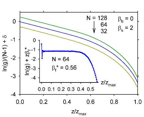
Figure 12: Densities of state for an adsorbing surface. The solid lines represent the normalized logarithm of the density of states $g(z;\beta_{s}=2,\beta_{b}=0)$ as a function of the normalized extension $z/z_{\mathrm{max}}$. To separate the graphs for the different chain lengths, constant values $\delta=0.25$, 0, -0.25 have been added to $\ln(g)$ for $N=128$, 64, and 32, respectively. The steps in $\ln(g)$ near $z=0$, evident for $N=32$ and clearly visible in the inset, are due to the discrete positions the chain end can assume on the lattice. The inset shows, for $N=64$ and the transition field $\beta_{f}^{*}=0.56$, the logarithm of the reweighted density of states, $g\exp(z\beta_{f}^{*})$, which is proportional to the canonical probability distribution.

For intermediate extensions, the graphs of $\ln(g)$ for $\beta_{s}=2$ are linear within the statistical uncertainties. The slope of the lines is nearly identical for all three chain lengths and the extension range where linear behavior is observed increases with increasing chain length. According to Eq. (18), the slope of a $\ln(g(z))$ graph represents the negative tension field as a function of extension. This implies that the extensions in the straight-line portions of the graphs all belong to the same tension field, which we call $\beta_{f}^{*}$. For $N=64$, we show in the inset of Fig. 12 the logarithm of the reweighted density of states, $g\exp(z\beta_{f}^{*})$, which, up to a normalization factor, represents the canonical probability distribution defined in Eq. (15). The discrete steps in the probability distribution at low extensions are now clearly visible. For intermediate extensions, we find a flat probability distribution, implying that conformations with a wide range of extensions have the same probability for being realized.

The extension results in Figs. 11 and 4 were obtained with a canonical evaluation of the density of states, according to Eqs. (16) and (17). In Fig. 13, we present results from a micro-canonical evaluation of the density of states for chains of length $N=64$ and $N=128$. The tension field $\beta_{f}$ is calculated from a numerical derivative of the logarithmic density of states according to Eq. (18), where the smallest extensions were omitted due to the discrete jumps in $g(z)$ discussed above. In Fig. 13, we show the graph with $\beta_{f}$ on the horizontal axis to facilitate comparison with the force extension-curves in Fig. 11 (a). In this representation, the region of constant slope of $\ln(g)$ becomes a vertical line at the transition field, $\beta_{f}^{*}\simeq 0.56$, and shows clearly the discontinuous nature of the transition. According to Eq. (19), the second derivative of $\ln(g)$ with respect to $z$ yields the inverse of the extension fluctuations. Since the first derivative of $\ln(g)$ is constant, we find that $\chi_{z}^{-1}$ vanishes in the coexistence region, corresponding to a $\delta$-function peak in $\chi_{z}$ at the transition field. This singularity is analogous to the $\delta$-peak in the isobaric heat-capacity at vapor-liquid coexistence and typical for discontinuous transitions.

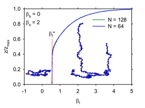
Figure 13: Force-induced desorption for surface-contact field $\beta_{s}=2$ and athermal solvent conditions, $\beta_{b}=0$. The solid lines represent results from a microcanonical evaluation of the densities of state for chain lengths $N=128$ and $N=64$. The vertical line segment indicates the tension field at the transition, $\beta_{f}^{*}=0.56$, and highlights the vertical part of the extension curve, which signals phase coexistence. The results for the two chain lengths are just barely distinguishable at the end of the coexistence region. The simulation snapshots show conformations for chains of length $N=64$; an adsorbed chain (left) and a set of conformations for the coexistence region (right).

Comparing the force-extension results in Fig. 13 with those obtained by a canonical evaluation of the density of states in Fig. 11 (a), we note that the results are in excellent agreement at high tensions and start to deviate only near the transition. In the canonical evaluation, where $\beta_{f}$ is controlled, the average extension is calculated as a weighted sum over all possible extensions. For finite systems, this leads to a broadening of the transition and a transition region, whose size decreases with increasing chain length. In the thermodynamic limit, where $N\rightarrow\infty$, both evaluation methods are expected to give identical results.

In contrast to other first-order transitions in finite-size systems (see, for example, the results for stretching chains from globular and crystalline phases in Sec. III.2.2) the probability distribution at the transition field is flat rather than bimodal, suggesting that a large number of states coexist at the transition field $\beta_{f}^{*}$ Skvortsov et al. (2012). As we discuss further in Sec. IV, this is due to the absence of an interfacial barrier between coexisting states. At the transition between adsorbed and stretched states, the coexistence is between adsorbed and stretched parts of the chain with a negligible interface between the domains. In the inset of Fig. 13 we show a set of such conformations for chain length $N=64$.

III.3.2 Phase portrait for finite chains near attractive surfaces

To investigate the relationship between tension and adsorption over a range of conditions, we present a phase portrait for chains of length $N=64$ in the $\beta_{f}-\beta_{s}$ plane of tension and surface contact fields in Fig. 14. We distinguish between two phases, adsorbed and desorbed, where the desorbed phase includes both expanded coil and stretched chain conformations.

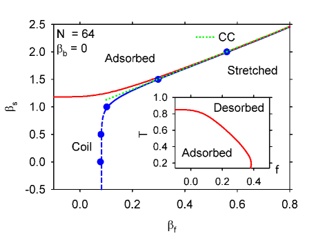
Figure 14: Phase portrait for tethered chains of length $N=64$ in the space of tension field, $\beta_{f}$, and surface-contact field, $\beta_{s}$. The solid and dashed lines show the location of fluctuation maxima, determined from an evaluation of the 3-d density of states $g(n_{s},n_{b},z)$. The red solid line delineating the region of adsorbed conformations represents maxima of surface-contact fluctuations, $\chi_{s}$. Desorbed chains have expanded coil and stretched conformations for low and high tension fields, respectively. The solid and dashed blue lines show maxima in extension fluctuations, $\chi_{z}$, which indicate the force-induced desorption transition at high $\beta_{s}$ (solid lines) but do not represent phase transitions for low $\beta_{s}$ (dashed lines). The filled symbols show inflection point results from Wang-Landau simulations at fixed $\beta_{s}$ and $\beta_{b}=0$. The dotted line labeled CC is a straight line with slope 1.9 estimated from a Clausius-Clapeyron relation. The inset shows the phase portrait in the force–temperature plane, where $T=1/\beta_{s}$ and $f=\beta_{f}/\beta_{s}$ for surface interaction energy $\epsilon_{s}=-1$.

The blue lines in Fig. 14 indicate maxima in the extension fluctuations, $\chi_{z}$. At low surface contact fields $\beta_{s}$, these maxima are not related to phase transitions and therefore a dashed line is used to show their location in the $\beta_{f}$-$\beta_{s}$ plane. The location of $\chi_{z}$ maxima is independent of $\beta_{s}$ for repulsive and slightly attractive surfaces. As $\beta_{s}$ approaches the adsorption value, $\beta_{sa}\simeq 1.18$ for $N=64$, chain stretching starts to interfere with adsorption. In the discussion of Fig. 11 (d) we noted that the surface-contact fluctuations as a function of $\beta_{f}$ first develop a maximum for $\beta_{s}\gtrsim 1.0$. Around this value, we see in Fig. 14 the line of $\chi_{z}$ maxima starting to move to higher tension fields and approach the line of $\chi_{s}$ maxima. The results presented in Figs. 12 and 13 show that the transition between adsorbed and stretched chains is discontinuous. For chains of length $N=64$, we find evidence for phase coexistence down to about $\beta_{s}=1.3$. The lines of fluctuation maxima at high fields therefore represent coexistence lines, whose slope may be estimated from a Clausius Clapeyron (CC) relation. For coexistence between adsorbed and stretched chains, the CC relation reads $d\beta_{s}/d\beta_{f}=-\Delta z/\Delta n_{s}$, where $\Delta z$ and $\Delta n_{s}$ are the differences in extension and number of surface contacts of the coexisting states, respectively. For $\beta_{s}=2.0$ we estimate a value of 1.9 for the slope, which is indicated by the dotted line in the figure and seen to give a good representation of the coexistence curve in the range shown here. As $\beta_{s}$ increases further, the slope increases and reaches a value of about 2.7 for the largest fields where we evaluate our data. In the limit $\beta_{s}\rightarrow\infty$, the slope is expected to approach a value of 3, since the largest bond length in the model is 3 and its value will be added to the extension each time a surface contact is broken.

The red solid line separating adsorbed conformations at high $\beta_{s}$ values from desorbed conformations at low $\beta_{s}$ values represents maxima in the surface contact fluctuations, $\chi_{s}$, which we use to identify the adsorption transition. At low tension fields, the adsorption transition is continuous and the line of $\chi_{s}$ maxima almost independent of $\beta_{f}$. For tension fields $\beta_{f}\gtrsim 0.1$, the adsorption transition moves to higher $\beta_{s}$ values and for fields $\beta_{f}\gtrsim 0.2$, we find evidence for phase coexistence. The phase diagram has a region where finite-size effects are particularly evident; for $N=64$ it is the area $1.0\lesssim\beta_{s}\lesssim 1.6$ and $0.1\lesssim\beta_{f}\lesssim 0.4$. In this region, the transition field values obtained from maxima in surface-contact and extension fluctuations are not the same (see Fig. 11) leading to a gap between the transition lines. A comparison with results from other chain lengths shows that size of the region where the lines approach each other decreases with increasing chain length.

In the inset of Fig. 14, we present the line of adsorption transitions in the more familiar force-temperature plane. For the conversion, we set $\epsilon_{s}=-1$ for the interaction energy, which yields $T=1/\beta_{s}$ and $f=\beta_{f}/\beta_{s}$. In this representation, the chain is adsorbed at low temperatures and forces and desorbs by increasing temperature or tension force. The adsorption transition is continuous at low forces and high temperatures and becomes discontinuous as the tension increases. Near the lowest temperatures accessible to us, the phase diagram shows reentrant behavior, in agreement with theoretical predictions and simulation results in the literature, (see, for example, Refs. [Skvortsov et al., 2012; Bhattacharya et al., 2009a]).

III.3.3 Effect of solvent condition on force-induced desorption

To investigate the effect of solvent condition on force-induced desorption, we performed 1-d Wang-Landau simulations for chains of length $N=64$ tethered to an adsorbing surface, $\beta_{s}=2$ in near-$\theta$ ($\beta_{b}=0.5$) and poor ($\beta_{b}=0.7$) conditions. In the absence of tension, these surface and solvent conditions yield adsorbed extended chain conformations.Luettmer-Strathmann et al. (2008) This means that even though a desorbed chain at $\beta_{b}=0.7$ is collapsed, the adsorbed chain is in an extended quasi-two dimensional conformation. Compared to athermal solvent conditions ($\beta_{b}=0$) the lateral extension of an adsorbed chain in poor solvent is smaller and the perpendicular extension is slightly larger as a result of competition between bead-bead and surface contacts.

In Fig. 15 we present data for the densities of state for $\beta_{b}=0$, $\beta_{b}=0.5$, and $\beta_{b}=0.7$. The inset of Fig. 15 shows a chain conformation in the transition region for $\beta_{b}=0.7$, which may be compared with athermal-solvent conformations in Fig. 13. For all solvent conditions, the results show an extended range of extensions, where $\ln(g)$ decreases linearly. As discussed in Sec. III.3.1 (see Figs. 12 and 13) this implies coexistence of states at a transition field $\beta_{f}*$, which is given by the negative slope of the graphs. We find values of $\beta_{f}*=0.56$, 0.64, and 0.73 for the solvent conditions $\beta_{b}=0$, 0.5, and 0.7, respectively.

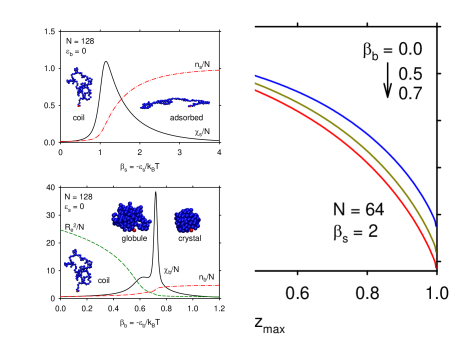
Figure 15: Densities of state for an adsorbing surface, $\beta_{s}=2$, and three different solvent conditions for chains of length $N=64$. The solid lines represent the logarithm of the normalized density of states $g(z;\beta_{s},\beta_{b})$ as a function of the normalized extension $z/z_{\mathrm{max}}$ for athermal solvent, $\beta_{b}=0$, near $\theta$ solvent, $\beta_{b}=0.5$, and poor solvent $\beta_{b}=0.7$. The simulation snapshot shows a chain conformation in the transition region (linear part of the graph) for $\beta_{b}=0.7$.

In Fig. 16 (a) we present force-extension results from the canonical evaluation of the densities of state; the inset shows extension fluctuations in the transition region. The graphs confirm that the transition field increases with increasing $\beta_{b}$ and that the transition is sharpest for the athermal solvent. Panel (b) shows the bead-bead and surface contact numbers in the transition region. The initial number of surface contacts is largest for the chain in athermal solvent and smallest for poor-solvent conditions. Conversely, bead contact numbers are smallest in athermal solvent and largest in poor solvent. As the tension increases, both types of contact numbers decrease first gradually and then rapidly as the chain undergoes the transition to the stretched state.

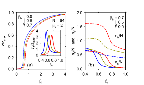
Figure 16: Force-induced desorption in good and poor solvent. (a) Normalized extension $z/z_{\mathrm{max}}$ as a function of tension field, $\beta_{f}$, for adsorbing surface, $\beta_{s}=2.0$, and increasingly poorer solvent, $\beta_{b}=0$, 0.5, and 0.7 for $N=64$; the inset shows the normalized extension fluctuations, $\chi_{z}/z_{\mathrm{max}}$, in the transition region. (b) Normalized surface contacts, $n_{s}/N$, (solid lines) and bead contacts, $n_{b}/N$, (dashed lines) in the transition region.

To summarize, force-induced desorption in poor solvent occurs at higher tension than in good solvent conditions. The nature of the transition is discontinuous with a broad range of coexisting states for chains that are stretched from adsorbed extended initial states.

IV Summary and conclusion

In this work, we developed a simulation approach to investigate tethered chain molecules subject to an applied tension force. To describe systems with a broad range of surface interactions and solvent conditions, we employed a bond-fluctuation lattice model with bead-surface and bead-bead interactions, where the effect of solvent interactions is included implicitly in the interaction parameters of the model. The thermodynamic properties of the chains are completely determined by the density of states $g(n_{s},n_{b},z)$ over the three-dimensional state space of surface contacts ($n_{s}$), bead-bead contacts ($n_{b}$), and extensions ($z$); the fields conjugate to these quantities are the bead-contact field $\beta_{b}=-\epsilon_{b}/T$, the surface contact field $\beta_{s}=-\epsilon_{s}/T$, and the tension field $\beta_{f}=f/T$, where $f$ is the applied force. For fixed surface and bead contact fields, the 1-d density of states $g(z;\beta_{s},\beta_{b})$ determines the force-extension relations of the chains.

With the aid of the Monte Carlo simulation techniques described in Appendix A, we constructed $g(n_{s},n_{b},z)$ for chains of length $N=32$, 64, and 128. Force-extension curves calculated from $g(n_{s},n_{b},z)$ are most reliable for low to intermediate tension fields. They allow us to investigate tethered chains for continuously varying solvent and surface conditions and thereby identify states of interest. For selected solvent and surface conditions, we performed Wang-Landau simulations at fixed $\beta_{s}$ and $\beta_{b}$ to determine the 1-d density of states $g(z;\beta_{s},\beta_{b})$ as described in Appendix  B. These simulations provide access to the high tension regime and allow us to study details of phase transitions under tension. To validate the method, we compared with scaling laws in the low and intermediate force regime and exact results in independent-bond (IB) approximation for high tensions. We find that our simulation results are consistent with scaling and IB predictions.

Single-chain pulling experiments give insight into the effect of solvent conditions on the mechanical response of chain molecules. Since simple polymer models, such as the freely-jointed chain Grosberg and Khokhlov (1994) and the wormlike chain Bustamante et al. (1994); Marko and Siggia (1995); Bouchiat et al. (1999), have fixed solvent conditions, we wanted to explore if our coarse-grained model is able to describe force-extension relations over the wide range of conditions, where experiments have been performed. In the intermediate force regime, the force-extension curve has universal properties that allow us to compare our model with comparatively short chains to experiments on long biological chain molecules. The contour length and the characteristic segment length connect the model to the biomolecule and are determined from simulation results and experimental data, respectively. The remaining model parameter describes the solvent condition and is estimated from a comparison with experimental data. We obtain a good qualitative description of the experimental data except at the highest tensions (see Fig. 6), where the bonds of the biological molecules become extensible Smith et al. (1996) requiring more detailed molecular models. Our experience suggests that the computational method presented in Appendix B can be applied without prohibitive computational cost to obtain force-extension relations for more realistic models of biomolecules in good to moderate solvents and thus become a useful tool to interpret rupture-type single-molecule experiments.

In poor solvent conditions, a sufficiently large pulling force stretches the chain out of the globular state. In agreement with theoretical predictions and experimental observation, our model yields first-order transitions from the globule to the stretched state for long chains (see Fig. 7). We also find that the tension field at the stretching transition increases linearly with increasing bead-contact field (see Fig. 9), which is consistent with experimental results by Li et al.Li and Walker (2010) For force-induced transitions from states with crystalline order we discovered that there is no intermediate globular state; instead, we find coexistence between crystalline and stretched conformations and transition states, where crystallites and stretched chain sections coexist on the same chain (see Fig. 8). Our results for the effect of solvent condition on the stretching transition and the effect of tension on chain collapse and crystallization are summarized in the phase portrait presented in Fig. 9.

To study the effects of surface attractions, we start with athermal solvent conditions ($\beta_{b}=0$) and vary the surface contact field $\beta_{s}$. Slightly attractive surface interactions lead to a distortion of the expanded coil conformations found near hard surfaces and to force-extension relations that are very similar to those of hard surfaces. For adsorbing surfaces, a small applied force changes only the conformation of the unadsorbed tail of the chain, whose size is independent of the chain length $N$ and decreases with increasing surface attraction. This leads to zero-force extensions, $z_{0}$, and inverse spring constants, $\chi_{z0}$, that are independent of the chain length and decrease with increasing $\beta_{s}$ (see Figs. 4 and 11).

The transition between adsorbed and stretched states is discontinuous with a flat (rather than bimodal) probability distribution at the transition field $\beta_{f}^{*}$. The negative logarithm of the probability distribution is the variational free energy. Normally, first order transitions in finite systems lead to bimodal distribution functions, which yield free energy functions with two minima corresponding to the two coexisting phases. However, the “hump” in between the minima is due to interfacial contributions in the mixed phase region of the finite system. In our case, however, the “interface” is not an extended object, but corresponds to a single monomer only, and hence there is no free energy cost due to the interface for phase coexistence here. Our findings for the transition are consistent with those of Skvortsov et al. Skvortsov et al. (2012), who discuss the nature of the desorption transition in detail. We have also performed simulations in $\theta$ and poor solvent conditions, where the chains are in adsorbed extended states in the absence of tension, and find that, while force-induced desorption occurs at higher tension than in good-solvent conditions, the nature of the transition is unchanged.

The phase portrait in Fig. 14 illustrates the relation between adsorption and chain stretching. For weakly adsorbing surfaces, we find expanded coil conformations that become stretched (without passing through a phase transition) with increasing tension field. At high $\beta_{s}$, the chains are adsorbed and undergo a discontinuous transition to stretched states with increasing $\beta_{f}$. The adsorption transition at low tension is continuous and little affected by the tension field $\beta_{f}$, until $\beta_{f}$ is sufficiently large to desorb the chains. While finite-size effects are evident in the region where adsorption and chain stretching first interfere with each other, we expect the general conclusions drawn from this work to be applicable in the long-chain limit.

Appendix A Construction of the 3-d density of states $g(n_{s},n_{b},z)$

In the absence of tension, a state of the system is described by the pair of contact numbers $(n_{s},n_{b})$, where the accessible contact numbers form a two-dimensional state space. Luettmer-Strathmann et al. (2008) The density of states, $g(n_{s},n_{b})$, defined as the number of chain conformations (micro states) for state $(n_{s},n_{b})$, contains the complete information about the equilibrium thermodynamics of the system. In earlier work, we employed Wang-Landau algorithms Wang and Landau (2001b); Landau et al. (2004); Zhou et al. (2006) to construct the density of states $g(n_{s},n_{b})$ over the two-dimensional state space of monomer-monomer and monomer-surface contacts for tethered chains in the absence of tension for chain lengths up to $N=64$ Luettmer-Strathmann et al. (2008) and $N=128$. The elementary moves for the simulations consisted of displacement of individual beads to nearest-neighbor sites, pivot moves about the $z$ axis, and so-called cut-and-permute moves, where the chain is cut at a random bead, top and bottom are interchanged, and the chain is reassembled and tethered to the surface if the move is accepted.Causo (2002) For our simulations of tethered chains over a two-dimensional state space, we employed several different strategies to find the 2-d density of states $g(n_{s},n_{b})$, within reasonable computation times Luettmer-Strathmann et al. (2008). For each chain length, at least two independent densities of states were generated and extensively umbrella sampled to avoid systematic errors and achieve a quality that allows evaluation by numerical differentiation.

To construct $g(n_{s},n_{b},z)$ we take advantage of the fact that, up to an overall factor that cancels in the evaluations, the density of states $g(n_{s},n_{b},z)$ may be written as the product

$$g(n_{s},n_{b},z)=p(z;n_{s},n_{b})g(n_{s},n_{b}),$$ (21)

where $p(z;n_{s},n_{b})$ is the probability that the extension equals $z$ for given contact numbers $(n_{s},n_{b})$. To determine the probability distributions $p(z;n_{s},n_{b})$ we use the previously calculated 2-d density of states $g(n_{s},n_{b})$ Luettmer-Strathmann et al. (2008) in “production” simulations where we build histograms of the height $z$ of the last bead without updating $g(n_{s},n_{b})$. In practice, the probabilities $p(z;n_{s},n_{b})$ become very small for large values of $z$ and have large relative uncertainties, which restricts the evaluation of the 3-d density of states to states with very low tension forces. In order to improve the statistics for chain conformations with larger extensions, we performed production simulations under fixed field(s) and evaluated the results with histogram reweighting techniques. When only the tension field $\beta_{f}$ is fixed, the acceptance criterion for the simulations is

$$p\left((n_{s},n_{b},z;\beta_{f})\rightarrow(n^{\prime}_{s},n^{\prime}_{b},z^{\prime};\beta_{f})\right)\mbox{\hskip 30.00005pt}$$

$$=\min\left(\frac{g(n_{s},n_{b})}{g(n^{\prime}_{s},n^{\prime}_{b})}e^{-\beta_{f}(z-z^{\prime})},1\right),$$ (22)

where $z^{\prime}$ and $z$ are the last bead’s $z$-coordinate of the trial and original chain conformations, respectively. To improve sampling of partially desorbed or extended chains under tension, we also performed production simulations, where a contact field, for example the surface field $\beta_{s}$, is also held constant. In this case, the acceptance criterion becomes

$$p\left((n_{s},n_{b},z;\beta_{s},\beta_{f})\rightarrow(n^{\prime}_{s},n^{\prime}_{b},z^{\prime};\beta_{s},\beta_{f})\right)\mbox{\hskip 30.00005pt}$$

$$=\min\left(\frac{g(n_{s},n_{b})}{g(n^{\prime}_{s},n^{\prime}_{b})}e^{-\beta_{s}(n_{s}-n^{\prime}_{s})-\beta_{f}(z-z^{\prime})},1\right),$$ (23)

and similarly for fixed bead-contact field $\beta_{b}$. For chain lengths $N=16$, 32, and 128, production simulations with the acceptance criterion (22) were carried out for tension fields $\beta_{f}=0.0,0.1,\ldots,0.6$ and a few additional fields. To explore the effect of tension on adsorption and chain collapse, more extensive simulations were performed for chains of length $N=64$. Tension fields $\beta_{f}=0.0,0.1,\ldots,1.0$ were employed with Eq. (22) and simulations with acceptance criterion (23) were performed for a few $\beta_{f}$ values and surface fields up to $\beta_{s}=2.84$ as well as for fixed bead-contact fields up to $\beta_{b}=0.91$. Production simulations for finite tension typically have $10^{9}$ Monte Carlo steps, divided into ten blocks, where the first block is used for equilibration and results from the remaining nine blocks are evaluated to find the average profiles and uncertainties. For zero tension, the total production time is typically 10¹⁰ MC steps and all ten blocks are evaluated.

Histograms collected during the simulations yield values for the probability $p(z;n_{s},n_{b},\beta_{f})$ to find the last bead at height $z$ for given contact numbers $(n_{s},n_{b})$ and tension field $\beta_{f}$. To compensate for the applied field, the profiles $p(z;n_{s},n_{b},\beta_{f})$ are multiplied with $z$-dependent weights $e^{-\beta_{f}z}$. For each pair $(n_{s},n_{b})$, the reweighted profiles from different tensions are combined by applying constant shift factors to assure a good match in the overlap regions. In the process, data at the edges of the profiles are examined and data points with very large uncertainty are discarded. Finally, data derived from different tensions are averaged in their regions of overlap to arrive at the combined probability profiles $p(z;n_{s},n_{b})$, which are entered into Eq. (21) to determine the density of states $g(n_{s},n_{b},z)$ over the three-dimensional state space. In Fig. S2 of the supplementary material sup we present an example for a combined profile. These results illustrate how the technique of production under tension with reweighting extends the profile to much larger heights than are accessible in zero-tension simulations.

Appendix B 1-d densities of state

While the combination of profiles described above increases the range of accessible heights of the last bead, it is not sufficient to reach the most highly extended chain conformations. In order to explore the full range of tension forces and chain extensions we perform Wang-Landau simulations that sample all possible heights of the last bead at fixed surface and bead contact fields. The acceptance criterion for these simulations is

$$p\left((n_{s},n_{b},z;\beta_{s},\beta_{b})\rightarrow(n^{\prime}_{s},n^{\prime}_{b},z^{\prime};\beta_{s},\beta_{b})\right)\mbox{\hskip 40.00006pt}$$

$$=\min\left(\frac{g(z;\beta_{s},\beta_{b})}{g(z^{\prime};\beta_{s},\beta_{b})}e^{-\beta_{s}(n_{s}-n^{\prime}_{s})-\beta_{b}(n_{b}-n^{\prime}_{b})},1\right),$$ (24)

where $g(z;\beta_{s},\beta_{b})$ is the current estimate for the density of state for the one-dimensional state space of $z$ coordinates of the last bead for the given fields $\beta_{s}$ and $\beta_{b}$. For these simulations, the density of states is updated with the original Wang-Landau prescriptionWang and Landau (2001b); Landau et al. (2004) with refinement levels $f_{k}=\exp(2^{-(k-1)})$ for $k=4,5,\ldots,30$. We experimented with different flatness criteria and found that the traditional 80% rule works well for these simulations. We performed simulations for chains of length $N=16$, 32, 64, 128, and 256 for several contact fields. Typically, the density of states converged in simulations over the whole range of $z$. However, in cases where the range of probabilities is very large, for example for $N=256$, simulations were carried out in overlapping windows and their results combined to give the final density of states. For contact fields that lead to discontinuous stretching transitions, for example for $N=32$ and $\beta_{b}=2$, care must be taken that the entire coexistence region is covered by a window. Uncertainty estimates for the densities of states are obtained either from multiple independent simulations or by comparing results from the last few iteration levels.

In Fig. S3 of the supplementary material sup we present the 1-d density of states $g(z;\beta_{s},\beta_{b})$ for chain length $N=64$ and fields $\beta_{s}=\beta_{b}=0$ and compare it with the corresponding probability distribution, $p(z;\beta_{s},\beta_{b})$, calculated by partial summation of the 3-d density of states $g(n_{s},n_{b},z)$. The figure illustrates two typical observations. First, the 1-d density of states $g(z;\beta_{s},\beta_{b})$ extends smoothly to the highest possible extension, $z_{\mathrm{max}}=3(N-1)$, while $p(z;\beta_{s},\beta_{b})$ has a limited range and shows large statistical errors at higher extension. Secondly, in the range of $z$ values where both probabilities are available, $p(z;\beta_{s},\beta_{b})$ and $g(z;\beta_{s},\beta_{b})$ are in excellent agreement. In this work, we use 3-d and 1-d densities of states in a complimentary way: With results from $g(n_{s},n_{b},z)$, we investigate tethered chains for continuous ranges of the thermodynamic fields $\beta_{s}$, $\beta_{b}$, and $\beta_{f}$, we construct phase diagrams, and identify states of interest. For these, we perform 1-d Wang-Landau simulations to investigate their force-extension relations in detail, including the highest possible extensions.

Supplemental Material for: Transitions of tethered chain molecules under tension

Scaling of extension-fluctuation maxima with chain length

To discuss the significance of maxima in the extension fluctuations, we present in Fig. S1 chain-length dependent results for scaled fluctuation maxima, $\chi_{z}^{*}/z_{0}^{2}$, where $z_{0}$ is the zero-force extension. For athermal solvent, $\beta_{b}=0$, the fluctuation maxima $\chi_{z}^{*}$ occur in the low-force scaling region and are expected to scale with chain length in the same way as the zero-force fluctuations, i.e. $\chi_{z}^{*}\sim z_{0}^{2}\sim N^{2\nu}$ so that $\chi_{z}^{*}/z_{0}^{2}$ is expected to be independent of the chain length. This behavior is indeed observed for the $\beta_{b}=0$ data in Fig. S1. For $\beta_{b}=0.5$, the scaled fluctuation maxima in Fig. S1 are just starting to show an increase with increasing chain length. For poorer solvents, $\beta_{b}=0.6$ and $\beta_{b}=0.7$, $\chi_{z}^{*}/z_{0}^{2}$ grows markedly with $N$ implying that the fluctuation maxima grow much faster than the chain length. Since this is the expected behavior near phase transitions, these results suggest that chain stretching acquires the character of a phase transition as the solvent quality decreases.

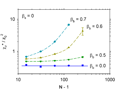
Figure S1: Scaled maxima of extension fluctuations $\chi_{z}^{*}/z_{0}^{2}$ as a function of chain length, $N-1$, for four solvent conditions, $\beta_{b}=0$, 0.5, 0.6, and 0.7. The symbols represent simulation results, the dashed lines are a guide to the eye. The solid line represents the average value of the simulation results for $\beta_{b}=0$.

Probability distributions from 1-d and 3-d densities of states

Fig. S2 illustrates the construction of the 3-d density of states.

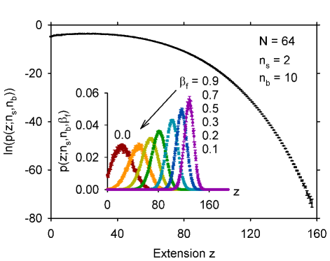
Figure S2: Logarithm of the combined probability profile $p(z;n_{s},n_{b})$ as a function of extension, $z$, for chain length $N=64$, $n_{s}=2$ surface contacts, and $n_{b}=10$ bead contacts. The symbols with error bars show the probability distribution obtained by reweighting profiles from production simulations under different fields. The combined profile shows that there is a good match between the reweighted probabilities in the overlap regions. The inset shows probability profiles $p(z;n_{s},n_{b},\beta_{f})$ (in linear scale) from simulations for seven different tension fields between $\beta_{f}=0.0$ and $\beta_{f}=0.9$ that contributed to the combined profile. As one would expect, with increasing tension force in the upward direction, the maximum of the probability shifts to larger extensions and the width of the profiles decreases. These results illustrate how the technique of production under tension with reweighting extends the profile to much larger heights than are accessible in zero-tension simulations; for the contact numbers in this figure, $n_{s}=2$, $n_{b}=10$, from a maximum height of about $z=60$ ($\beta_{f}=0.0$ profile in inset) to one of about $z=155$.

When the 1-d density of states is normalized to unity so that $\sum_{z}g(z;\beta_{s},\beta_{b})=1$, it represents the probability to find the last bead at height $z$ for contact fields $\beta_{s}$ and $\beta_{b}$. The probability distribution $p(z;\beta_{s},\beta_{b})$ for the extension at constant contact fields may also be calculated by partial summation of the 3-d density of states $g(n_{s},n_{b},z)$

$$p(z;\beta_{s},\beta_{b})=\frac{\sum_{n_{s},n_{b}}g(n_{s},n_{b},z)\mathrm{e}^{\beta_{s}n_{s}}\mathrm{e}^{\beta_{b}n_{b}}}{\sum_{n_{s},n_{b},z}g(n_{s},n_{b},z)\mathrm{e}^{\beta_{s}n_{s}}\mathrm{e}^{\beta_{b}n_{b}}}.$$ (S25)

In Fig. S3 we show a comparison of $p(z;\beta_{s},\beta_{b})$ and normalized $g(z;\beta_{s},\beta_{b})$ results.

Figure S3: Logarithm of the normalized density of states $g(z;\beta_{s},\beta_{b})$ for chain length $N=64$ and contact fields $\beta_{s}=\beta_{b}=0$. The largest possible extension, $z_{\mathrm{max}}=3(N-1)=189$, for this chain length is indicated by an arrow. The solid line represents results from one Wang-Landau simulation over the one-dimensional space of heights $z$; results from two other simulations are indistinguishable on this scale. The symbols with error bars represent the probability distribution $p(z;\beta_{s},\beta_{b})$ calculated with Eq. (S25) from the density of states $g(n_{s},n_{b},z)$ over the three-dimensional space of states $(n_{s},n_{b},z)$. The range of extensions for $p(z;\beta_{s},\beta_{b})$ is limited and the uncertainties at higher $z$ are large due to insufficient sampling of highly stretched chain conformations during the production simulations. In the range where both are available, $p(z;\beta_{s},\beta_{b})$ and $g(z;\beta_{s},\beta_{b})$ are in excellent agreement.

References

- Ritort (2006) F. Ritort, J. Phys.: Cond. Mat. 18, R531 (2006).
- Kumar and Li (2010) S. Kumar and M. S. Li, Physics Reports 486, 1 (2010).
- Evans and Ritchie (1997) E. Evans and K. Ritchie, Biophys. J. 72, 1541 (1997).
- Ray et al. (2007) C. Ray, J. R. Brown, and B. B. Akhremitchev, J. Phys. Chem. B 111, 1963 (2007).
- Dougan et al. (2009) L. Dougan, J. Li, C. J. Badilla, B. J. Berne, and J. M. Fernandez, Proc. Natl. Acad. Sci. USA 106, 12605 (2009).
- Vrbová and Whittington (1996) T. Vrbová and S. G. Whittington, J. Phys. A.: Math. Gen. 29, 6253 (1996).
- Rajesh et al. (2002) R. Rajesh, D. Dhar, D. Giri, S. Kumar, and Y. Singh, Phys. Rev. E 65, 056124 (2002).
- Krawczyk et al. (2005) J. Krawczyk, A. L. Owczarek, T. Prellberg, and A. Rechnitzer, Europhys. Lett. 70, 726 (2005).
- Bachmann and Janke (2006) M. Bachmann and W. Janke, Phys. Rev. E 73, 041802 (2006).
- Luettmer-Strathmann et al. (2008) J. Luettmer-Strathmann, F. Rampf, W. Paul, and K. Binder, J. Chem. Phys. 128, 064903 (2008).
- Binder et al. (2008) K. Binder, W. Paul, T. Strauch, F. Rampf, V. Ivanov, and J. Luettmer-Strathmann, J. Phys.: Condens. Matter 20, 494215 (2008).
- Möddel et al. (2011) M. Möddel, W. Janke, and M. Bachmann, Macromolecules 44, 9013 (2011).
- Knotts IV et al. (2008) T. A. Knotts IV, N. Rathore, and J. de Pablo, Biophys. J. 94, 4473 (2008).
- Heinz et al. (2009) H. Heinz, B. L. Farmer, R. B. Pandey, J. M. Slocik, S. S. Patnaik, R. Pachter, and R. R. Naik, J. Am. Chem. Soc. 131, 9704 (2009).
- Swetnam and Allen (2012) A. Swetnam and M. P. Allen, Phys. Rev. E 85, 062901 (2012).
- Radhakrishna et al. (2012) M. Radhakrishna, S. Sharma, and S. K. Kumar, J. Chem. Phys. 136, 114114 (2012).
- Bustamante et al. (1994) C. Bustamante, J. F. Marko, E. D. Siggia, and S. Smith, Science 265, 1599 (1994).
- Smith et al. (1996) S. B. Smith, Y. Cui, and C. Bustamante, Science 271, 795 (1996).
- Haupt et al. (2002) B. J. Haupt, T. J. Senden, and E. M. Sevick, Langmuir 18, 2174 (2002).
- Dessinges et al. (2002) M.-N. Dessinges, B. Maier, Y. Zhang, M. Peliti, D. Bensimon, and V. Croquette, Phys. Rev. Lett. 89, 248102 (2002).
- Cocco et al. (2003) S. Cocco, J. F. Marko, R. Monasson, A. Sarkar, and J. Yan, Eur. Phys. J. E 10, 249 (2003).
- Danilowicz et al. (2007) C. Danilowicz, C. H. Lee, V. W. Coljee, and M. Prentiss, Phys. Rev. E 75, 030902 (2007).
- Gunari et al. (2007) N. Gunari, A. C. Balazs, and G. C. Walker, J. Am. Chem. Soc. 129, 10046 (2007).
- Saleh et al. (2009) O. A. Saleh, D. B. McIntosh, P. Pincus, and N. Ribeck, Phys. Rev. Lett. 102, 068301 (2009).
- Li and Walker (2010) I. T. S. Li and G. C. Walker, J. Am. Chem. Soc. 132, 6530 (2010).
- Dittmore et al. (2011) A. Dittmore, D. B. McIntosh, S. Halliday, and O. A. Saleh, Phys. Rev. Lett. 107, 148301 (2011).
- Pincus (1976) P. Pincus, Macromolecules 9, 386 (1976).
- Halperin and Zhulina (1991a) A. Halperin and E. B. Zhulina, Europhys. Lett. 15, 417 (1991a).
- Halperin and Zhulina (1991b) A. Halperin and E. B. Zhulina, Macromolecules 24, 5393 (1991b).
- Marko and Siggia (1995) J. F. Marko and E. D. Siggia, Macromolecules 28, 8759 (1995).
- Ha and Thirumalai (1997) B.-Y. Ha and D. Thirumalai, J. Chem. Phys. 106, 4243 (1997).
- Bouchiat et al. (1999) C. Bouchiat, M. D. Wang, J.-F. Allemand, T. Strick, M. Block, and V. Croquette, Biophysical Journal 76, 409 (1999).
- Livadru et al. (2003) L. Livadru, R. R. Netz, and H. J. Kreuzer, J. Chem. Phys. 118, 1404 (2003).
- Bhattacharya et al. (2009a) S. Bhattacharya, V. G. Rostiashvili, A. Milchev, and T. A. Vilgis, Macromolecules 42, 2236 (2009a).
- Klushin and Skvortsov (2011) L. I. Klushin and A. M. Skvortsov, J. Phys. A: Math. Theor. 44, 473001 (2011).
- Skvortsov et al. (2012) A. M. Skvortsov, L. I. Klushin, A. A. Polotsky, and K. Binder, Phys. Rev. E 85, 031803 (2012).
- Wittkop et al. (1994) M. Wittkop, J.-U. Sommer, S. Kreitmeier, and D. Göritz, Phys. Rev. E 49, 5472 (1994).
- Wittkop et al. (1996) M. Wittkop, S. Kreitmeier, and D. Göritz, Phys. Rev. E 53, 838 (1996).
- Grassberger and Hsu (2002) P. Grassberger and H.-P. Hsu, Phys. Rev. E 65, 031807 (2002).
- Frisch and Verga (2002) T. Frisch and A. Verga, Phys. Rev. E 65, 041801 (2002).
- Celestini et al. (2004) F. Celestini, T. Frisch, and X. Oyharcabal, Phys. Rev. E 70, 012801 (2004).
- Morrison et al. (2007) G. Morrison, C. Hyeon, N. M. Toan, B.-H. Ha, and D. Thirumalai, Macromolecules 40, 7343 (2007).
- Bhattacharya et al. (2009b) S. Bhattacharya, V. G. Rostiashvili, A. Milchev, and T. A. Vilgis, Phys. Rev. E 79, 030802 (2009b).
- Toan and Thirumalai (2010) N. M. Toan and D. Thirumalai, Macromolecules 43, 4394 (2010).
- Hsu and Binder (2012) H.-P. Hsu and K. Binder, J. Chem. Phys. 136, 024901 (2012).
- Wang and Landau (2001a) F. Wang and D. P. Landau, Phys. Rev. Lett. 86, 2050 (2001a).
- Wang and Landau (2001b) F. Wang and D. P. Landau, Phys. Rev. E 64, 056101 (2001b).
- Paul et al. (2007) W. Paul, T. Strauch, F. Rampf, and K. Binder, Phys. Rev. E 75, 060801 (2007).
- Wüst et al. (2011) T. Wüst, Y. W. Li, and D. P. Landau, J. Stat. Phys. 144, 638 (2011).
- Taylor et al. (2009) M. P. Taylor, W. Paul, and K. Binder, J. Chem. Phys. 131, 114907 (2009).
- Decas et al. (2008) R. Decas, J.-U. Sommer, and A. Blumen, Macromol. Theory Simul. 17, 429 (2008).
- Grosberg and Khokhlov (1994) A. Y. Grosberg and A. R. Khokhlov, Statistical Physics of Macromolecules, AIP Series in Polymers and Complex Materials (American Institute of Physics, Woodbury, NY, 1994).
- Cifra and Bleha (1995) P. Cifra and T. Bleha, Macromol. Theory Simul. 4, 233 (1995).
- Brak et al. (2009) R. Brak, P. Dyke, J. Lee, A. L. Owczarek, T. Prellberg, A. Rechnitzer, and S. G. Whittington, J. Phys. A 42, 085001 (2009).
- Eisenriegler et al. (1982) E. Eisenriegler, K. Kremer, and K. Binder, J. Chem. Phys. 77, 6296 (1982).
- Carmesin and Kremer (1988) I. Carmesin and K. Kremer, Macromolecules 21, 2819 (1988).
- Binder (1995) K. Binder, Monte Carlo and Molecular Dynamics Simulations in Polymer Science (Oxford University Press, Oxford, 1995).
- Landau and Binder (2000) D. P. Landau and K. Binder, A Guide to Monte Carlo Simulations in Statistical Physics (Cambridge University, Cambridge, UK, 2000).
- (59) See Supplemental Material at the end of this manuscript for details on the scaling of the zero-force extension fluctuations and for figures illustrating the construction and validation of the density-of-states obtained by the algorithms described in the appendices.
- Rampf et al. (2005) F. Rampf, W. Paul, and K. Binder, Europhys. Lett. 70, 628 (2005).
- Ferrenberg and Landau (1991) A. M. Ferrenberg and D. P. Landau, Phys. Rev. B 44, 5081 (1991).
- Descas et al. (2004) R. Descas, J.-U. Sommer, and A. Blumen, J. Chem. Phys. 120, 8831 (2004).
- Landau et al. (2004) D. P. Landau, S.-H. Tsai, and M. Exler, Am. J. Phys. 72, 1294 (2004).
- Zhou et al. (2006) C. Zhou, T. C. Schulthess, S. Torbrügge, and D. P. Landau, Phys. Rev. Lett. 96, 120201 (2006).
- Causo (2002) M. S. Causo, J. Stat. Phys. 108, 247 (2002).