Studies of the Jet in BL Lacertae. II. Superluminal Alfvén Waves

Abstract

We study the kinematics of ridge lines on the pc-scale jet of the active galactic nucleus BL Lac. We show that the ridge lines display transverse patterns that move superluminally downstream, and that the moving patterns are analogous to waves on a whip. Their apparent speeds $\rm\beta_{app}$ (units of $c$) range from 3.9 to 13.5, corresponding to $\rm\beta_{wave}^{gal}=0.981-0.998$ in the galaxy frame. We show that the magnetic field in the jet is well-ordered with a strong transverse component, and assume that it is helical and that the transverse patterns are Alfvén waves propagating downstream on the longitudinal component of the magnetic field. The wave-induced transverse speed of the jet is non-relativistic ($\rm\beta_{tr}^{gal}\mathrel{\mathchoice{\lower 2.0pt\vbox{\halign{$\nms\displaystyle\hfil#\hfil$\cr<\crcr\sim\crcr}}}{\lower 2.0pt\vbox{\halign{$\nms\textstyle\hfil#\hfil$\cr<\crcr\sim\crcr}}}{\lower 2.0pt\vbox{\halign{$\nms\scriptstyle\hfil#\hfil$\cr<\crcr\sim\crcr}}}{\lower 2.0pt\vbox{\halign{$\nms\scriptscriptstyle\hfil#\hfil$\cr<\crcr\sim\crcr}}}}0.09$). In 2010 the wave activity subsided and the jet then displayed a mild wiggle that had a complex oscillatory behaviour. The Alfvén waves appear to be excited by changes in the position angle of the recollimation shock, in analogy to exciting a wave on a whip by shaking the handle. A simple model of the system with plasma sound speed $\rm\beta_{s}=0.3$ and apparent speed of a slow MHD wave $\rm\beta_{app,S}=4$ yields Lorentz factor of the beam $\rm\Gamma_{beam}\sim 4.5$, pitch angle of the helix (in the beam frame) $\alpha\sim 67^{\circ}$, Alfvén speed $\rm\beta_{A}\sim 0.64$, and magnetosonic Mach number $\rm M_{ms}\sim 4.7$. This describes a plasma in which the magnetic field is dominant and in a rather tight helix, and Alfvén waves are responsible for the moving transverse patterns.

1. Introduction

This is the second in a series of papers in which we study high-resolution images of BL Lacertae made at 15 GHz with the VLBA, under the MOJAVE program (Monitoring of Jets in Active Galactic Nuclei with VLBA Experiments, Lister et al., 2009). In Cohen et al. (2014, hereafter Paper I) we investigated a quasi-stationary bright radio feature (component) in the jet located 0.26 mas from the core, (0.34 pc, projected) and identified it as a recollimation shock (RCS). Numerous components appear to emanate from this shock, or pass through it. They propagate superluminally downstream, and their tracks cluster around an axis that connects the core and the RCS. This behavior is highly similar to the results of numerical modeling (Lind et al., 1989; Meier, 2012), in which MHD waves or shocks are emitted by an RCS. In the simulations, the jet has a magnetic field that dominates the dynamics, and is in the form of a helix with a high pitch angle, $\alpha$. In BL Lac the motions of the components are similar to those in the numerical models, and in addition the Electric Vector Position Angle (EVPA) is longitudinal; i.e., parallel to the jet axis. For a jet dominated by helical field, this indicates that the toroidal component is substantial ($\rm B_{\phi}/B_{pol}\mathrel{\mathchoice{\lower 2.0pt\vbox{\halign{$\nms\displaystyle\hfil#\hfil$\cr>\crcr\sim\crcr}}}{\lower 2.0pt\vbox{\halign{$\nms\textstyle\hfil#\hfil$\cr>\crcr\sim\crcr}}}{\lower 2.0pt\vbox{\halign{$\nms\scriptstyle\hfil#\hfil$\cr>\crcr\sim\crcr}}}{\lower 2.0pt\vbox{\halign{$\nms\scriptscriptstyle\hfil#\hfil$\cr>\crcr\sim\crcr}}}}1$), a necessary condition for the comparison of the observations with the numerical simulations. Hence, in Paper I, we assumed that the superluminal components in BL Lac are compressions in the beam established by slow- and/or fast- mode magnetosonic waves or shocks traveling downstream on a helical field.

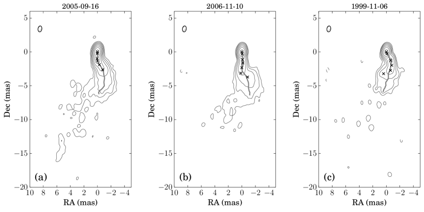
Figure 1.— 15 GHz VLBA images of BL Lac with ridge line and components (the crosses). In (a) the components lie close to the ridge line. In (b) the three outer components are off the ridge line by up to 0.3 mas. In this case the true ridge has a sharp bend and the algorithm has difficulty in following it. In (c) the ridge has a step near the core, and appears to bifurcate downstream. The algorithm misses the step, and is unable to deal with the bifurcation.

It has been common to assume that the EVPA is perpendicular to the projection of the magnetic field vector B that is in the synchrotron emission region. This is correct in the frame of an optically-thin emission region, but may well be incorrect in the frame of the observer if the beam is moving relativistically (Blandford & Königl, 1979; Lyutikov, Pariev, & Gabuzda, 2005). Lyutikov, et al. show that if the jet is cylindrical and not resolved transversely, and if the B field has a helical form, then the EVPA will be either longitudinal or perpendicular to the jet, depending on the pitch angle. This is partly seen in the polarization survey results of Lister & Homan (2005), where the BL Lac objects tend to have longitudinal EVPA in the inner jet, whereas the quasars have a broad distribution of EVPA, relative to the jet direction. This suggests that in BL Lacs the field may be helical, with pitch angles large enough to produce longitudinal EVPA, although strong transverse shocks in a largely tangled field are also a possibility (e.g. Hughes, 2005). The wide distribution of EVPA values in quasars suggests that oblique shocks, rather than helical structures, might dominate the field order. However, a distribution of helical pitch angles could also explain the EVPAs in quasars, if symmetry is broken between the near and far sides of the jet. It has been suggested (Meier, 2013) that this difference in the magnetic field is fundamental to the generic differences between quasars and BL Lacs and, by inference, between Fanaroff & Riley Class II and I sources, respectively (Fanaroff & Riley, 1974).

BL Lacs often show a bend in the jet, and the literature contains examples showing that in some cases the EVPA stays longitudinal around the bend; e.g., 1803+784; Gabuzda (1999), 1749+701; Gabuzda & Pushkarev (2001), and BL Lac itself; O’Sullivan & Gabuzda (2009). In these examples the fractional polarization $p$ rises smoothly along the jet to values as high as $p=30\%$. The field must be well-ordered for the polarization to be that high. In this paper we assume that the field is in a rather tight helix (in the beam frame) and that the moving patterns (the transvese disturbances) are Alfvén waves propagating along the longitudinal component of the field.

In a plasma dominated by the magnetic field, Alfvén waves are transverse displacements of the field (and, perforce, of the plasma), analogous to waves on a whip. The tension is provided by the magnetic field $\rm(\propto B^{2})$, and the wave velocity is proportional to the square root of the tension divided by the (relativistic) mass density. Alfvén waves have been employed in various astronomical contexts, including the acceleration of cosmic rays (Fermi, 1949), the solar wind (Belcher, Davis & Smith, 1969), the Jupiter-Io system (Goldreich & Lynden-Bell, 1969), turbulence in the ISM (Goldreich & Sridhar, 1997), the bow shock of Mars (Edberg et al., 2010), and the solar atmosphere(McIntosh et al., 2011). In our case they are transverse waves on a relativistically-moving beam of plasma threaded with a helical magnetic field. The appropriate formulas for the phase speeds of the MHD waves are given in the Appendix of Paper I.

Changes in the ridge lines of BL Lacs are also seen frequently. Britzen et al. (2010a) showed that in 1.4 years the BL Lac object 0735+178 changed from having a “staircase” structure to being straight, and that there were prominent transverse motions. Britzen et al. (2010b) also studied 1803+784 and described various models that might explain the structure. Perucho et al (2012) studied the ridge line in 0836+710 at several frequencies and over a range of epochs. They showed that the ridge line corresponds to the maximum pressure in the jet. They discussed the concept of transverse velocity, and concluded that their measured transverse motions are likely to be caused by a “moving wave pattern”; this was elaborated in Perucho (2013). In our work here on BL Lac we also see transverse motions, but their patterns move longitudinally and we identify them as Alfvén waves. We calculate the resulting transverse velocity of the wave motion and show that it is non-relativistic.

It has been more customary to discuss the fast radio components in a relativistic jet in hydrodynamic (HD) terms. We note here only a few examples of this. The shock-in-jet model (Marscher & Gear, 1985; Marscher, 2014) was used by Hughes, Aller, & Aller (1989a, 1989b, 1991) to develop models of several sources, including BL Lac (Hughes, Aller, & Aller, 1989b) and 3C 279 (Hughes, Aller, & Aller, 1991). Lobanov & Zensus (2001) recognized two threads of emission in 3C 273 that they explained with Kelvin-Helmholtz instabilities, and this was developed more by Perucho et al. (2006). Hardee, Walker & Gómez (2005) discussed the patterns and motions in 3C 120 in terms of helical instability modes. In all these studies the magnetic field is needed of course for the synchrotron radiation, but it also is explicitly used to explain observed polarization changes as due to compression of the transverse components of magnetic field by the HD shock. But in these works the magnetic field has no dynamical role in the jet. On the contrary, in this paper, as in Paper I, we assume that the dynamics in the jet are dominated by the magnetic field.

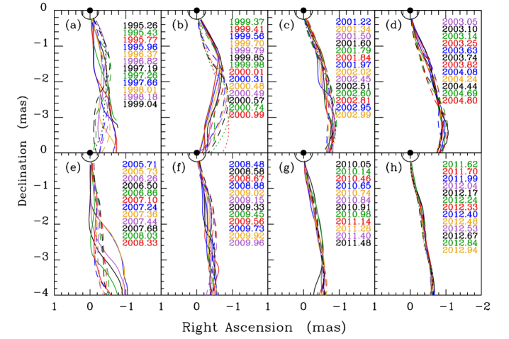
Figure 2.— Ridge lines for BL Lac, 1995.26 - 2012.94. Successive panels are adjacent in time. Epochs are identified by color. In each panel the first occurence of a color is further identified as the solid line, the next occurence as a dashed line, and the third occurence, when it exists, as a dotted line. The core is shown as the solid dot, and the semi-circle is drawn 0.25 mas from the core. In all cases the RCS is close to the circle.

The plan for this paper is as follows. In Section 2 we briefly describe the observations. The definition of the ridge line of a jet is considered in Section 3, and the transverse waves and their velocities, including the behavioral change in 2010, are presented and discussed in Section 4. Excitation of the waves by changes in the P.A. of the RCS is considered in Section 5. In Section 6 we identify the waves as Alfvén waves, discuss their properties, and present simple models of the system.

For BL Lac $z=0.0686$, and the linear scale is $\rm 1.29~{}pc~{}mas^{-1}$. An apparent speed of $\rm 1~{}mas~{}yr^{-1}$ corresponds to $\rm\beta_{app}=4.20$.

2. Observations

For this study of BL Lac we use 114 epochs of high-resolution observations made with the VLBA at 15 GHz, between 1995.27 and 2012.98. Most of the observations (75/114) were made under the MOJAVE program (Lister & Homan, 2005), a few were taken from our earlier 2-cm program on the VLBA (Kellermann et al., 1998), and the rest were taken from the VLBA archive.

The data were all reduced by the MOJAVE team, using standard calibration programs (Lister et al, 2009). Following the reduction to fringe visibilities we calculated three main products at nearly every epoch:

(1)

An image, consisting of a large number of “clean delta functions” produced by the algorithm used for deconvolution, convolved with a “median restoring beam”, defined in Section 3.

(2)

A model, consisting of a set of Gaussian “components” found by model-fitting in the visibility plane; each component has a centroid, an ellipticity, a size (FWHM), and a flux density. The Gaussians are circular when possible. The total set of components sums to the image, but in this paper we only use components that have been reliably measured at four or more epochs, have flux density $\rm>20~{}mJy$, and can be tracked unambiguously from epoch to epoch. A typical epoch shows 4-6 of these “robust” components. The RCS is a permanent component and, together with the core, usually produces more than half of the total flux density from the jet. The centroids of the robust components for each epoch are plotted on the images in Figure 1.

The centroid locations are measured relative to the core, which we take to be the bright spot at the north end of the source; it usually is regarded as the optically-thick ($\tau=1$) region of the jet. In principle, the core can move on the sky. We considered this in Paper I, and concluded that any motions are less than $\rm 10~{}\mu as$ in a few years, and they were ignored. Our positional accuracy is conservatively estimated as $\rm\pm 0.1~{}mas$, and in this paper we again ignore any possible core motions.

(3)

The ridge line, shown in Figure 1 and discussed in Section 3.

The image, the components, and the ridge line are not independent, but each is advantageous when discussing different aspects of the source. In most cases the ridge line runs down the smallest gradient from the peak of the image, and the centroids of the components lie on the ridge line. However, when the jet has a sharp bend the algorithm can fail, as in Figure 1c. This is discussed in Section 3.

The components move in a roughly radial direction, and plots of $r(t)$ as well as the sky (RA–Dec) tracks are shown in Paper I and in Lister et al (2013). The tracks cluster around an axis at $\mathrm{P.A.}=-166^{\circ}$ and appear to emanate from a strong quasi-stationary component, C7, that we identified as a recollimation shock (RCS) in Paper I. The moving components have superluminal speeds; the fastest has $\rm\beta_{app}=10\pm 1$ in units of the speed of light. (Lister et al, 2013)

3. The Ridge Lines

We are dealing with moving patterns on the jet of BL Lac, and in order to quantify them we first need to define the ridge line of a jet. At least four definitions have been used previously. Britzen et al. (2010b) used the line that connects the components at a single epoch, in studying 1803+784. Perucho et al (2012) investigated three methods of finding the ridge line: at each radius making a transverse Gaussian fit and connecting the maxima of the fits, using the geometrical center, and using the line of maximum emission. They found no significant differences among these procedures, for the case they studied, 0836+710. They showed that the intensity ridge line is a robust structure, and that it corresponds to the pressure maximum in the jet.

To quantify a ridge line we start with the image as in Figure 1, which is the convolution of the “clean delta functions” with a smoothing beam. Since we are comparing ridge lines from different epochs, we have used a constant “median beam” for smoothing, and not the individual (“native”) smoothing beams. The latter vary a little according to the observing circumstances for each epoch, and their use would effectively introduce “instrumental errors” into the ridge lines. The median beam is a Gaussian with $\rm major~{}axis=0.89~{}mas~{}(FWHM),~{}minor~{}axis=0.56~{}mas$ and $\mathrm{P.A.}=-8\fdg 6.$ Each of the three parameters is the median of the corresponding parameters for all the epochs.

The algorithm for the ridge line starts at the core, and at successive steps (0.1 mas) down the image finds the midpoint, where the integral of the intensity across the jet, along a circular arc centered on the core, is equal on the two sides of the arc. The successive midpoints are then smoothed with a third-order spline.

Ridge lines are shown on the three images in Figure 1. In Figure 1a the bends in the jet are gradual and the algorithm works very well, as indeed would any of the methods mentioned above. In Figure 1b there are two sharp bends and our algorithm makes a smooth line that misses the corners of the bends. In this case connecting the components would be better, if the modelling procedure actually put components at the corners. In Figure 1c the jet appears to bifurcate, and our algorithm picks the west track. In this case a visual inspection of the image is required to see what is going on.

In fact there is another problem with Figure 1c. The image has a step to the east (looking downstream) about 1 mas from the core, where a short EW section connects two longer NS sections. Since the restoring beam is nearly NS the details of this step cannot be reconstructed. The calculated ridge line in Figure 1c does not reproduce the step, but makes a smooth track.

Figure 3.— Ridge line for $2005-09-16$ calculated (a) with native beams and (b) with median beam. Solid line: using all the antennas, dotted line: omitting SC and HN. In (a) the beam P.A.s differ by 17^∘.

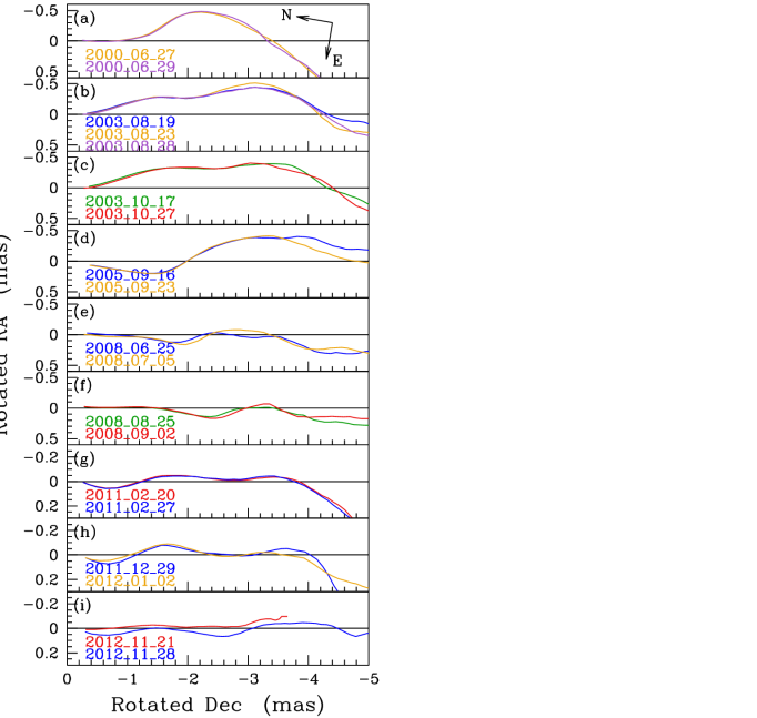
Figure 4.— Ridge lines for 10 pairs that each occur close in time. The axes are rotated from (RA, Dec) by $9\fdg 5$; North and East are indicated at top. The bottom 3 panels have a different vertical scale than the others, and the coordinate directions are thereby changed by a small amount.

Figure 2 shows nearly all the ridge lines that we consider in this paper; a few are not shown because they occur very close in time to another one. In all cases the RCS is located close to the semi-circle, drawn 0.25 mas from the core. Successive panels are adjacent in time, although there is a 1-yr gap in the data between panels (d) and (e). The only other substantial data gap is seen in panel (a), from 1998.18 to 1999.04. In Figure 2 the epochs are set nearly equally among the panels, with the separations picked to emphasize the various waves that are discussed below.

It is important to establish the reliability of the ridge lines because our analysis rests on them, and some of the structures that we interpret as waves are smaller than the synthesized VLBA beam. We first note that as with all VLBI our sampling of the $(u,v)$ plane is sparse, and different samplings can produce different ridge lines. To see how strong this effect is, we emulated an observation with missing antennas by analyzing a data set with and without one and two antennas, and we did this analysis both with the native restoring beams and the median restoring beam described above. The results for 2005-09-16 are shown in Figure 3; they are similar to the results we obtained for two other epochs. In Figure 3a we show two ridge lines, the solid one is calculated with the full data set and the dashed line is obtained when data from the SC and HN antennas are omitted. The latter calculation does not use many of the baselines, including the longest ones. The chief effect is a shift of the pattern downstream, by roughly 0.1 mas. This shift is not a statistical effect, but is mainly due to the different smoothing beams that were used for the two cases. We found that the differences in the ridge lines increased with increasing difference in the P.A.s of the smoothing beams. In Figure 3a the difference in P.A of the smoothing beams is 17^∘.

In Figure 3b we used the median beam. In this case the curves are close with differences of typically $3~{}\mu$as out to 4 mas, where the surface brightness becomes low. Beyond 4 mas the differences rise to $50~{}\mu$as.

Another way to investigate the reliability of the ridge lines is to examine pairs of ridge lines measured independently but close together in time. The full data set contains 10 pairs where the separation is no more than 10 days, and these are all shown in Figure 4. They are calculated with the median restoring beam. Note that the bottom three panels have a different vertical scale than the others. In general the comparison is very good within 4 mas of the core. Panel (i) contains one ridge line that stops at 3.6 mas because the brightness at the ridge becomes too low; this limit also can be seen in a few places in the other figures. Panel (i) contains the only pair that has a continuous offset, $\rm 30-50~{}\mu as$. These data were taken during an exceptional flux outburst at 15 GHz in BL Lac, seen in the MOJAVE data (unpublished), and roughly coincident with outbursts seen at shorter wavelengths (Raiteri et al., 2013). An extra coreshift leading to a position offset is expected with such an event (Kovalev et al., 2008; Pushkarev et al., 2012). In any event, this pair appears to be different from the others, and we do not include it in the statistics.

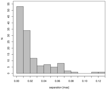
Figure 5.— Histogram of separations between members of 9 close pairs of ridge lines. The pairs are shown in Figure 4 but panel (i) is not included in the histogram. See text.

Figure 5 shows the histogram of separations between the paired ridge lines, after excluding those in panel (i) of Figure 4. In forming the ridge lines a 3-pixel smoothing was used, and for the histogram we have used every third point. The median separation is $\rm 13~{}\mu as$. Thus the repeatability of the ridge lines is accurate to about $\rm 13~{}\mu as$. The reliability also depends on the effect discussed in connection with Figure 1, that the ridge-finding algorithm can smooth around a corner, and can be in error by perhaps $\rm 100~{}\mu as$. However, the error is roughly constant over short time spans, as in Figure 4 panel (e) where the sharp bend at $\rm\sim 1.5~{}mas$ is smoothed the same in the two curves. This smoothing will have little effect on calculations of wave velocity, which is our main quantitative use of the ridge lines. We ignore the smoothing in this paper.

From this investigation we conclude that caution must be taken in interpreting the ridge lines, especially when comparing ridge lines obtained at different epochs, or with different frequencies. The details of the restoring beam can have a noticeable effect on the ridge line, and to avoid misinterpretation the restoring beam should be the same for all the ridge lines that are being intercompared.

When considering these ridge lines it is important to keep the geometry in mind: the jet has a small angle to the line-of-sight (LOS), and the foreshortening is about a factor of 10 (Paper I). Also, the projected images in Figure 1 can hide three-dimensional motions. To work with skew and non-planar disturbances, we use the coordinate systems shown in Figure 6. East, North, and the LOS form the left-hand system (x,y,z) and the jet lies at angle $\theta$ from the LOS in the $sagittal~{}plane$ formed by the LOS and the mean jet axis. This plane is perpendicular to the sky plane and is at angle P.A. from the $y$ axis. The rotated system $(\xi,\eta,\zeta)$ is used to describe transverse motions: $\xi$ is in the sagittal plane, $\eta$ is perpendicular to it, and $\zeta$ is along the jet. By “transverse motion” we mean that a point on the beam has a motion in the $(\xi,\eta)$ plane: $v_{\xi},v_{\eta}$. The component $v_{\xi}$ lies in the sagittal plane and its projection on the sky is along the projection of the jet. This component therefore is not visible, although a bright feature moving in the $\xi$ direction might be seen as moving slowly along the jet. However, the $v_{\eta}$ component remains perpendicular to the LOS as $\theta$ or P.A. changes, and its full magnitude is always seen. Thus a measured transverse motion is a lower limit. If the beam is relativistic then time compression of the forward motion must be added; see Section 4.3.

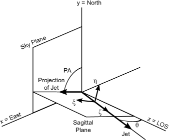
Figure 6.— Coordinate system. The sagittal plane is defined as the plane containing the LOS and the mean jet axis; see text.

Some of the panels in Figure 2 show disturbances that appear to move down the jet, and at other epochs the jet is fairly quiet. We now consider several of the disturbances in detail, starting with the structures seen in Figure 2, panel (b).

4. Waves on the Ridge Lines

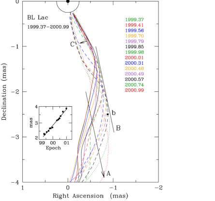
Figure 7.— Ridge lines for BL Lac at 15 GHz, for 14 epochs between 1999.37 and 2000.99. Below $r=-2$ mas, the displacement in space corresponds to a displacement in time, and the inset shows the points where the vector A crosses the ridge lines – the ordinate is distance along the vector A. The velocity in the A direction is $\rm 0.92~{}mas~{}yr^{-1}~{}at~{}P.A.=-167^{\circ}$; the arrow itself represents the propagation vector that is derived in the text. The offset straight line B is parallel to the propagation vector. It is approximately tangent to the wave crests, and so the wave has constant amplitude as it moves to the SW. The short arrow C shows a swing of the jet from west to east in early 2000; see text Section 5. The point $b$ shows the characteristic point on the 2000.57 line where the slope changes; see text Section 4.2. Colors are as in Figure 2.

Figure 7 is an expanded view of Figure 2, panel (b). It includes ridge lines for 14 consecutive epochs over a period of about 1.6 yr. Beyond 1 mas the early epochs (solid lines) show the jet bending to the SE. Later epochs show the bend farther downstream, and at 2000.31 and later the jet bends to the SW before bending SE. We anticipate a result from Section 4.2 and draw vector A at $\mathrm{P.A.}=-167^{\circ}$ across the tracks. The intersections of vector A with the tracks are shown in the inset in Figure 7. The velocity implied by the line in the inset is close to $\rm 1~{}mas~{}yr^{-1}$ or $\rm\beta_{app}\approx 4$. The pattern on the ridge line is moving superluminally downstream at nearly constant velocity. We consider three possible explanations for this.

1) We see the projection of a conical pattern due to a ballistic flow from a swinging nozzle, like water from a hose. The argument against this is that line B in Figure 7 is parallel to vector A and approximately tangent to the western crest; this feature of the ridge lines is not radial from the core as it would be if it were a ballistic flow. In Figure 2 all the panels except (a), (b), and (e) show clearly that the excursions of the ridge lines are constrained to lie in a cylinder, not a cone.

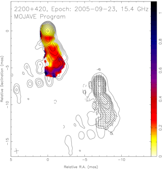
Figure 8.— Polarization image for BL Lac epoch 2005-09-23, one of those forming the large wave in Figure 10. Linear polarization fraction $p$ is indicated by the color bar; at the core $p\approx 6\%$, in the slice at $\sim-2~{}\rm{mas}~{}\it{p}$ drops to 15%, and on the ridge $p$ remains near 30% from 2 to 4 mas. In the right-hand image tick marks show the EVPA corrected for Galactic Faraday Rotation; the EVPA stays nearly parallel to the jet out to about 5 mas.

2) The moving pattern is due to a helical kink instability that is advected downstream with the flow. In the kink the field would be stretched out and become largely parallel to the observed bends in the jet that, in this case, seem to be transverse waves (Nakamura & Meier, 2004; Mizuno, Hardee, & Nishikawa, 2014). This would produce an EVPA normal to the wave crest in Figure 7 rather than longitudinal. But in BL Lac the EVPA tends to be longitudinal, even along the bends. In Figure 8 we show the polarization image for 2005-09-23, taken from the MOJAVE website¹. Similar polarization images for BL Lac, at several wavelengths, are shown in O’Sullivan & Gabuzda (2009, Figure 19) for epoch 2006-07-02. Both of these epochs are part of the large Wave D shown later in Figure 10. In these polarization images the EVPA is nearly parallel to the jet out to about 5 mas and $p$ is high on the ridge, indicating that the magnetic field remains in a relatively tightly-coiled helix around the bend and is not nearly parallel to the axis, as it should be for an advected kink instability.

Wave D is the largest wave in the BL Lac data, and seems to have the cleanest longitudinal polarization. At other epochs the EVPA tends to be longitudinal, but can be off by up to 40^∘. We have only one epoch of polarization data for Wave A, but that one does show an EVPA that is tightly longitudinal in the bend. Thus we believe that the EVPA results preclude the identification of the structures seen in Figure 7 as due to a kink instability.

3) The moving patterns are transverse MHD waves; i.e., Alfvén waves. For this to be possible the plasma must be dynamically dominated by a helical magnetic field. This condition for the jet of a BL Lac has been suggested many times; see e.g., Gabuzda, Murray & Cronin (2004), Meier (2013). Note that we implicitly assumed the helical, strong-field case in discussing the kink instability, in the preceding paragraph, and we also assumed it in Paper I. Thus, we assume that the moving pattern under vector A in Figure 7 is an Alfvén wave, with velocity $\rm\sim 1~{}mas~{}yr^{-1}$.

In Figure 7 a second wave is seen between $r=1$ and $r=2$ mas, where the ridge lines for epochs 2000.31 and later bend to the SW. The two waves in Figure 7 can be thought of as one wave with a crest to the west. This wave is generated by a swing of the nozzle to the west followed by a swing back to the east about 2 years later, as discussed below in Section 5.

The 1999-2000 wave is displayed in a different form in Figure 9, which shows the ridge lines from 1999.37 to 2001.97. Vertical spacing is proportional to epoch, and the axes have been rotated by 13^∘; arrows at top show North and East. Tick marks on the right are 0.1 mas apart. The dots show the points described later in Section 4.2, where the slope changes, and the solid line A is a linear fit through the points, with speed $v=0.92\pm 0.05\rm{~{}mas~{}yr^{-1}}$. This wave is prominent until 2000.99. In 2001.22 the structure has changed. There are alternate possibilities to explain this new structure, B. It may be a new wave, with the crests connected with line B (drawn with the same slope as line A). In this case the wave must have been excited somehow far from the RCS. The fit of line B to the wave crests is poor and would be improved if acceleration were included, but there is not enough data for that. Alternatively, structure B may simply be a relic of the trailing side of wave A, perhaps relativistically boosted by the changing geometry (the bend) seen in Figure 2 panel (c). A third wave C is shown by the dashed line that again is drawn with the same slope.

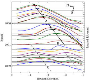
Figure 9.— Ridge lines for 1999.37-2001.97, plotted on axes rotated by 13^∘. North and East are indicated at the top. The ridge lines are spaced vertically according to epoch, and the tick marks on the right-hand side are spaced 0.1 mas apart. The solid line is a linear fit to the dots, which are the characteristic points discussed in Section 4.2. The three lines are parallel and all have slope 0.92 mas $\rm yr^{-1}$. See text.

Panel (c) of Figure 2 shows the ridge lines projected on the sky for 2001 – 2002. Wave B from Figure 9 is seen as the bump to the east at $r=2$ mas, which moves downstream at succeeding epochs. The projected axis of the jet is curved at these epochs, and the possible acceleration noted above for wave B may simply be a relativistic effect inherent in the changing geometry.

Wave A in Figure 9 is barely visible in Figure 2 panel (a) as a gentle bump in 1999.04, so it is first apparent in early 1999 at a distance $r\sim 1$ mas from the core. This is reminiscent of the behavior of the components discussed in Paper I; Figure 3 of that paper shows that most of the components first become visible near $r=1$ mas. Wave C also appears to start near $r\sim 1$ mas.

In Figure 7 the short arrow C shows an eastward swing of the inner jet between 2000.01 and 2000.31. This is seen in Figure 9 in the ridge line for 2000.31, which shows a new inner P.A. The effect of these P.A. swings on the beam is discussed in Section 5.

The different panels in Figure 2 show that the jet can be bent, and even when relatively straight, can lie at different P.A.s. Hence there is no unique rotation angle for the ridge lines in a plot such as that in Figure 9. The rotation angle used in Figure 9 was found by the velocity algorithm described in Section 4.2 for wave A.

Further examples of waves are shown in $\rm Figures~{}\ref{fig:ridge0506}-\ref{fig:ridge0909}$, omitting the extraneous ridge lines to avoid confusion. The wave motions are indicated by the arrows, which are propagation vectors derived in Section 4.2. Table 1 lists the details for these waves. $v$ is the measured proper motion, $\rm\beta_{app}$ is the apparent speed in units of $c$, $\rm\beta_{wave}^{gal}$ the wave speed in the coordinate frame of the galaxy, assuming $\theta=6^{\circ}$, and P.A. is the projected direction of the propagation vector. The amplitude is an estimate of the projected distance (in mas) across the wave, perpendicular to the propagation vector. Wave D is the largest such feature seen in the data. Unfortunately, there was an 11-month data gap prior to 2005.71, and the wave cannot be seen at earlier times.

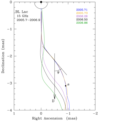
Figure 10.— Ridge lines for BL Lac at 15 GHz, for 5 epochs between 2005.7 and 2006.9. The propagation vector for Wave D is at $\rm{P.A.}=-180^{\circ}$.

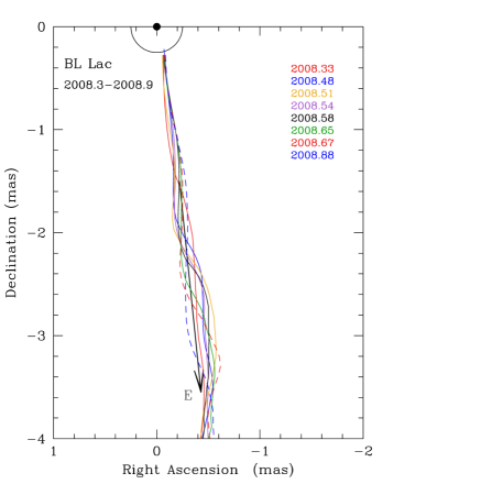
Figure 11.— Ridge lines for BL Lac at 15 GHz, for 7 epochs between 2008.5 and 2008.9, showing Wave E with a propagation vector at $\rm{P.A.}=-175^{\circ}$.

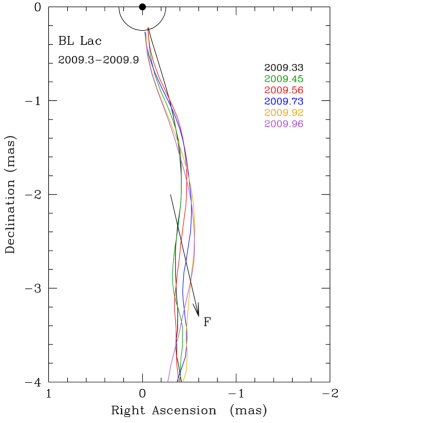
Figure 12.— Ridge lines for BL Lac at 15 GHz, for 6 epochs between 2009.3 and 2009.9, showing Wave F with propagation vector at $\rm{P.A.}=-166^{\circ}$.

The amplitudes of the larger waves appear to be comparable with the wavelength, as suggested for example by the inclination angle $\psi$ shown in Figure 10: $\psi\approx 36^{\circ}$. But this is an illusion caused by the foreshortening, which is approximately a factor of 10 (Paper I), so the deprojected value of $\psi$ is about 5^∘. Note that this is a lower limit, since the transverse motion can have a component in the $(\xi,\zeta)$ plane in Figure 6.

Figure 13 contains one frame of a movie of BL Lac showing the jet motions and ridge line fits at 15 GHz. The full movie is available in the electronic version of this paper.

Table 1Transverse Waves on the Jet of BL Lac.

Epoch	N	$v$		$\beta_{app,T}$	$\beta^{gal}_{wave}$	P.A.		Amplitude
		(mas y-1)				(deg)		(mas)
A 1999.37-2000.99	14	0.92	$\pm.05$	3.9	0.979	$-167.0$	$\pm 1.4$	0.5
D 2005.71-2006.86	5	1.25	$\pm.11$	5.6	0.987	$-180.2$	$\pm 1.1$	0.9
E 2008.33-2008.88	8	3.01	$\pm.16$	13.5	0.998	$-174.2$	$\pm 0.7$	0.3
F 2009.33-2009.96	6	1.11	$\pm.19$	5.0	0.985	$-167.1$	$\pm 2.4$	0.2

• Notes. Columns are as follows: (1) Wave label, (2) Inclusive range of epochs, (3) number of epochs, (4) apparent speed, (5) error, (6) apparent speed in units of $c$, (7) speed in galaxy frame, assuming $\theta=6^{\circ}$, (8) P.A. of the wave, (9) error, (10) estimated amplitude.

Figure 13.— Movie of the BL Lac jet at 15 GHz. The total intensity image is on the right, with a color bar indicating flux density. The contour levels begin at 7 mJy per beam, and increase by logarithmic factors of 2. The false color scheme uses a square root transfer function, and is saturated at the core position in order to highlight changes in the much fainter jet. The core peak brightness is highly variable; typically it is between 2 and 6 Jy/beam. The projected linear scale is indicated by the 2 pc line at left. The movie frames are linearly interpolated between the individual VLBA epoch images, which have been registered to the fitted position of the core feature, and restored with a median beam with FWHM dimensions of $0.89\times 0.57$ mas, with a major axis position angle at $-8\fdg 6$, as indicated in the lower left corner of the frame. The fitted ridge line is shown as a dashed line in the image, and again as a solid line to the left of the image. These have also been linearly interpolated between the individual VLBA epochs. The points of changing slope (see Section 4.2) at individual VLBA epochs are shown as the small symbols. At left the ridge lines are shown with different colors for the various waves. The yellow $v=c$ line on the right is advancing at the speed of light ($\beta_{\mathrm{app}}=1$) and is included for reference. The entire movie is available in the web version of this paper.

4.1. Different Jet Behavior in 2010-2013

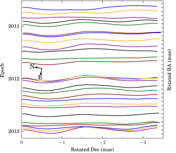
Figure 14.— Ridge lines as in Figure 2 panels (g) and (h), plotted on axes rotated by $9\fdg 5$ and with vertical spacing proportional to epoch. Tick marks on right-hand side are 0.1 mas apart.

In Figure 2 panels (g) and (h) we see that by 2010 the earlier transverse wave activity in the jet has subsided, and that after 2010.5 the jet is well-aligned at $\rm P.A.=-170\fdg 5$ with a weak wiggle. But the wiggle is not stationary. Figure 14 shows the ridge lines plotted on axes rotated by 9$\fdg$5, and spaced proportionately to epoch. Most of the ridge lines have a quasi-sinusoidal form. Almost all the epochs show a negative peak in the inner jet, with a minimum near $r=-0.7~{}{\rm mas}$. This is a quasi-standing feature, of variable amplitude. At most epochs there is a positive peak near $r=-1.6~{}{\rm mas}$. This also is a quasi-standing feature, but less distinct than the inner one.

What is causing the quasi-standing features? The patterns can hardly be true standing waves because that requires a reflection region. A rotating helix would project as a traveling wave, as on a barber pole, so a simple barber-pole model is excluded. Possible motions of the core are only about $\rm 10~{}\mu as$ (Paper I), so any registration errors due to core motion are much smaller than the observed changes, which are up to $\rm 100~{}\mu as$. There is little indication of wave motion in Figure 14, at least not at the speeds seen in Figure 2. It appears then, that during the period 2010-2013, the jet was essentially straight but with a set of weak quasi-stationary patterns, with variable amplitude.

4.2. Velocity of the Waves

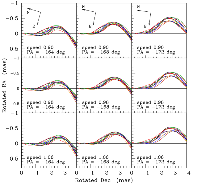
Figure 15.— Ridge lines shifted and overlaid on a grid of propagation vectors, for the 14 epochs shown in Figure 7. Each panel shows the assumed P.A. and the speed in mas s^-1; the P.A. is constant in the columns and the speed is constant in the rows. The axes are rotated to bring the P.A. to horizontal; North and East are shown at the top. See text.

We estimated the velocity of Wave A in Figure 7 in two independent ways. In the first we assume that there is a constant propagation vector, and we shift and superpose the ridge lines on a grid of ($v$, P.A.) where $v$ is the speed of the wave and P.A. is its propagation direction. If the ridge lines form a simple wave, then the solution is found when the lines lie on top of each other. This is shown in Figure 15, where a reasonable fit can be selected by eye. The result is $v=0.98\pm 0.08~{}\rm{mas~{}yr^{-1}}$ at $\rm P.A.=-168^{\circ}\pm 4^{\circ}$. This solution is somewhat subjective and the quoted errors do not have the usual statistical significance.

As an alternative procedure to visually aligning the ridge lines, we developed a method of identifying a characteristic point on the wave, just downstream of the crest, where the wave amplitude has begun to decrease. Define the slope of the ridge line as $\Delta x/\Delta y$ in pixels, where in Figure 9, $x$ and $y$ are rotated RA and Dec, and take the first downstream location where the slope exceeds $\pm 0.05$. This point is marked with the dot $b$ on the ridge line for 2000.57 in Figure 7. The $x$ and $y$ positions vs time for these locations are then fit independently using the same methods as described in Lister et al (2009) to extract a vector proper motion for this characteristic point on the wave.

The two methods agree well and the analytic solution is $v=0.92\pm 0.05~{}\rm{mas~{}yr^{-1}}$ at $\rm P.A.=-167\fdg 0\pm 0\fdg 5$, and the apparent speed is $\rm\beta_{app}=3.9\pm 0.2$. The propagation vector is shown in Figure 7 and the speed and direction of the wave are listed in Table 1. The Table also includes $\beta^{gal}_{wave}$ the speed of the wave in the galaxy frame, assuming $\theta=6^{\circ}$. This calculation assumes that the ridge lines lie in a plane; i.e., are not twisted. This is not neccessarily the case. Rather, since the inner jet, near the accretion disk, may wobble in 3 dimensions, (McKinney et al, 2013) it seems likely that the RCS may execute 3-dimensional motion and that the downstream jet will also. See Section 5.

Note that the P.A. of the first and last propagation vectors in Table 1 (-167$\fdg$0, -167$\fdg$1) is the same (to within the uncertainties) as the P.A. of the axis (-166$\fdg$6) defined in Paper I as the line connecting the core with the mean position of the recollimation shock. In the context to be developed later, the jet acts as a whip being shaken rapidly at the RCS, and tension in the whip continually pulls it towards the mean PA.

In Table 1 the speeds for the first, second and fourth waves are all similar at $\rm\beta_{app}\sim 5$, but Wave E (2008) is 3 times faster. Wave E has $\rm\beta_{app,E}\approx 13.5$, which is comparable to the speed for the fastest component in BL Lac, $\rm\beta_{app}\approx 10$, although the components speeds vary widely, from $\rm\beta_{app}\approx 2$ to $\rm\beta_{app}\approx 10$ (Lister et al, 2013). Wave E is also distinguished by its polarization; the EVPA is transverse not longitudinal like the others. We defer further discussion of Wave E to another paper.

4.3. Transverse Velocity

The ridge waves are relativistic transverse waves with apparent speeds $\rm\beta_{app}$ from 3.9 to 13.5 times the speed of light, and we assume that they have a small amplitude. From the usual formula for apparent speed,

$${\rm\beta_{app,wave}=\frac{\beta_{wave}^{gal}\sin{\theta}}{1-\beta_{wave}^{gal}\cos{\theta}}}$$ (1)

and taking values of $\rm\beta_{app,T}$ from Table 1 and using $\theta=6^{\circ}$, we find $\beta^{gal}_{wave}=0.979-0.998$ for the speed of the waves in the frame of the host galaxy. We now discuss the jet motion in terms of the coordinate system $(\xi,\eta,\zeta)$ shown in Figure 6.

Consider a transverse motion that is in the ($\eta,\zeta$) plane. Let the beam contain a co-moving beacon that is at the origin and emits a pulse at time $t^{\prime}=0$, where $t^{\prime}$ is in the coordinate frame of the galaxy. When $t^{\prime}=1$ yr the signal from the origin will have traveled $\rm 1\,ly$ down the z axis, towards the observer. Also at $t^{\prime}=1$ the beacon has moved from the origin to the point $(\eta,\zeta)=(\beta_{\mathrm{tr}},\beta_{\mathrm{beam}})$ where $\beta_{\mathrm{tr}}$ is the transverse speed, and $\beta_{\mathrm{beam}}$ is the longitudinal speed of the beam, both in the frame of the galaxy. At this point the beacon emits a second signal that also travels at the speed of light. In the z-direction, this signal trails the first one by ($1-\beta^{\mathrm{gal}}_{\mathrm{beam}}\cos\theta$) years. The apparent transverse speed of the beacon in the direction perpendicular to the jet, in the galaxy frame, is then

$${\beta_{\mathrm{app,tr}}=\frac{\beta_{\mathrm{tr}}}{(1-\beta^{\mathrm{gal}}_{\mathrm{beam}}\cos\theta)}}$$ (2)

and is to be differentiated from the apparent speed $\beta_{\mathrm{app}}$ commonly used in studies of superluminal motion, which is the apparent speed along the jet. Note the close relation between Equations 1 and 2. Equation 2 can be inverted to find $\rm\beta_{tr}$, a lower limit to the transverse speed.

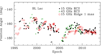
Figure 16.— Position Angle $vs$ Epoch for the RCS at 15 and 43 GHz, and for the Ridge Line at $r\approx 1$ mas. Epoch a represents the advected start of Wave D; see text.

For Wave A in Figure 7 we obtain an estimate for the transverse speed at $r\sim 2$ mas by taking the transverse motion as 0.5 mas and the time interval as $(2000.57-1999.41)$ yr, giving $v_{\rm tr}\approx 0.43~{}{\rm mas~{}yr}^{-1}$ and $\rm\beta_{app,tr}=1.9$ and, from Equation 2 with $\theta=6^{\circ}$ and $\rm\Gamma_{beam}=3.5$ (Paper I), $\beta^{\mathrm{gal}}_{\mathrm{tr}}\sim 0.09$. This is a model-dependent rough value, but it shows that the transverse speed is non-relativistic. This is necessary for consistency, since the derivation of the relativistic form of the MHD wave speeds shown in Paper I assumes that the velocity perturbation is small.

5. Excitation of the Waves

We suggested in Paper I that Component 7 is a recollimation shock, and that the fast components emanate from it. If this is correct, then the RCS should be a nozzle and its orientation should dictate the direction of the jet. In this Section we investigate this possibility. We first note that it is not possible to make a detailed mapping between the P.A. of the RCS and the later wave shape, for two reasons. First, the algorithm for the ridge line smooths over 3 pixels (0.3 mas), and thus smooths over any sharp features in the advected pattern. The second reason is more speculative. Our conjecture is that the wave is launched by plasma flowing through the nozzle and moving close to ballistically until its direction is changed by a swing in the P.A. of the nozzle. But magnetic tension in the jet continually pulls it towards the axis, and this means that it will bend, and that small-scale features will be stretched out and made smooth.

We start by comparing the P.A. of the RCS with the P.A. of the downstream ridge line at $r=1$ mas. Figure 16 shows the P.A. of the RCS measured at 15 GHz and at 43 GHz. The latter is calculated from data kindly provided by the Boston University VLBI group. We used the result found in Paper I, that the 15 GHz core is a blend of the first two 43 GHz components and that the 15 GHz component 7 is the RCS, as is the third 43 GHz component. We calculated the centroid of the first two 43 GHz components, to find an approximate position for the 15 GHz core, and then calculated the P.A. of the 43 GHz RCS from that centroid. The result is shown in Figure 16. We eliminated one discrepant point at 43 GHz, which was separated by about 20^∘ from nearby 43 GHz points, and one discrepant point at 15 GHz. The correspondence between the two frequencies is generally good, especially after 2005.0 where the agreement is typically within 3^∘. This further justifies our claim (Paper I) that the the location of this component is independent of frequency, and that it is a recollimation shock.

Figure 16 also contains the P.A. of the 15 GHz ridge line, close to $r=$ 1.0 mas. Between 2005.0 and 2010.0 the ridge line P.A. lags the RCS PA, by roughly 0.6 to 1.5 yr. After 2010 the PA of both the RCS and the ridge line stabilizes, and the subsequent variations, with rms amplitude about 3^∘, may mainly be noise. Prior to 2005.0 the variations are faster and more frequent and the lag is erratic. In places there appears to be no lag, but around 2000.0 and again around 2004.0 it is about 0.5 yr. Thus it appears that the swinging in PA of the RCS is coupled to the transverse motions of the ridge line. When the RCS is swinging rapidly and strongly, as before 2005, then so also is the ridge at 1 mas, with an irregular lag in P.A. that sometimes is about a half a year, and at other times is negligible. But when the RCS is swinging more slowly, as after 2005, then the ridge at 1 mas is also swinging slowly, with a lag of about a year, and after 2010.0 they both are stable, with only small motions that may be dominated by measurement errors.

We suggest that the large transverse waves on the ridge are excited by the swinging in P.A. of the RCS. Consider Wave A, seen in Figure 7. Its crest lies near line B and moves downstream at $\rm 0.92~{}mas~{}yr^{-1}$. In 1999.37 the crest is at about $r=1.2$ mas and at $\rm 0.92~{}mas~{}yr^{-1}$ would have been at the RCS ($r=0.25$ mas) around 1998.3. This is in a data gap at 15 GHz, but at 43 GHz there was a peak in P.A. in mid- or late-1998. Given that in 1999 the time lag between the RCS and the ridge at 1 mas apparently was much less than 1 yr, the association between the peak in the RCS P.A. in 1998 and the crest of Wave A is plausible. The fall in P.A. in 1999 and 2000 is seen as the short arrow C in Figure 7, and it corresponds to the upstream side of Wave A. The downstream side is the advected rise in P.A. of the RCS from mid-1997 to the peak in mid-or late 1998. The P.A. of the RCS fell from mid-1996 to mid-1997, and we might expect to find a corresponding crest to the east on Wave A, about 1 mas downstream of the main crest to the west. In fact several of the earliest ridge lines in Figure 7 do show a minor crest to the east at about $r=3.2$ mas, which is 2 mas or 2 years at 0.92 mas y^-1, downstream of the main crest to the west. A substantial acceleration in the wave speed would be needed for this to match. In any event, we cannot speculate usefully on this because it takes place beyond 3 mas, where there is a general bend to the east at all epochs. We conclude that a plausible association can be made between the large swing west then east of the RCS between 1998.0 and 2000.1, and Wave A that is later seen on the ridgeline.

A similar connection can be made for Wave D, seen in Figure 10 in 2005–2006. It can plausibly be attributed to the large swing of the RCS to the east that began in 2004 and continued into 2005. This wave does not have a crest as Wave A does, but a crude analysis can be made as follows. Assume that point $a$ on the 2005.71 ridge line is the advected beginning of the wave. With a speed of 1.25 mas y^-1 (Table 1) this means that the swing to the east began around 2003.5. This date is indicated on the abscissa in Figure 16. Apart from one high point at 2004.1 the P.A. of the RCS falls gradually from 2003.1 until late 2004, when it must fall abruptly to meet the first point after the data gap in 2005. This also is seen in Figure 10; the first four epochs have ridge lines that lie together and are straight at $\rm P.A.\approx-180^{\circ}$ out to $>1$ mas. This is consistent with the RCS P.A. being stationary from roughly 2004.7 to 2005.7 at $\sim-180^{\circ}$. This is in a data gap, and this analysis suggests that the RCS P.A. was $\approx-180^{\circ}$ during most or all of the gap. We conclude that the large swing in P.A. of the RCS from mid-2003 until mid-2005 generated Wave D, the largest wave in our data set.

The P.A. of the RCS rose rapidly from 2005.7 to about 2006.5, but the P.A. of the ridge line rose more slowly, and not as far. From 2007.0 to 2009.0 the P.A. of the inner jet was roughly constant at about -170^∘, while the P.A. of the RCS slowly dropped to the same value. We do not have a straightforward interpretation of this behavior. We also see in Figure 2 panels (e), (f) and (g) that following the passage of Wave D the jet slowly straightened out. The P.A. of the inner jet $(\sim-170^{\circ})$ propagated as a low-amplitude wave, at roughly the same speed as the large waves, $\rm\sim 1~{}mas~{}yr^{-1}$.

As a further complication, during this slow straightening out of the jet we see two more low-amplitude waves. The high-speed Wave E (Figure 11) has no obvious antecedent in the P.A. of the RCS. Wave F (Figure 12) is seen a year after Wave E, at the “usual” speed of 1.1 mas y^-1. These waves together make a complex set of possibly twisted ridge lines, seen together in Figure 2 panel (f).

In Section 4.1 we showed that the waves on the jet subsided in 2010, and in 2010-2012 the ridge line had only a weak variable wiggle. During this time the P.A. of the RCS was essentially constant; the variations seen in Figure 16 may represent the errors in the measurements, which would be about $\pm 3^{\circ}$. These variations in space and time have some regularities, as discussed in Section 4.1, but they do not appear to have a connection to the P.A. of the RCS.

In Paper I we saw that the component tracks all appear to come from or go through the RCS (component 7) and that they lie in a window centered on $\rm{P.A.}\approx-166^{\circ}$ (Caproni, Abraham, & Monteiro, 2012). This now is understood in terms of the waves on the ridge lines, since the components all lie on a ridge. The jet is analagous to a whip with a fixed mean axis being shaken with small amplitudes, in various transverse directions. The whip will occupy a narrow cylinder centered on the axis, and in projection the cylinder becomes our window.

6. Alfvén Waves and the BL Lac Whip

6.1. The Transverse Waves as Alfvén MHD Waves Along the Longitudinal Field Component

In Paper I we showed that the magnetic field in the jet of BL Lac has a strong transverse component. We assumed that it has a helical form, and that it is likely that the field dominates the dynamics in the jet. This is the condition for the existence of MHD waves that propagate down the jet. We suggested that the moving synchrotron-emitting components are compressions set up by fast and/or slow magnetosonic waves, possibly shocks. Now we introduce the third branch of MHD waves in the jet plasma, the Alfvén wave, which is a transverse S (shear) wave, with the disturbance occurring normal to the propagation direction. In Section 4 we showed that the moving patterns on the jet are transverse waves, and now we suggest that they are Alfvén waves.

The phase speed of a transverse Alfvén wave is given by

$${\beta_{T}=\pm\beta_{A}\cos\chi}$$ (3)

where $\beta_{A}=V_{A}/c$ is the relativistic scalar Alfvén speed, given in Equation A6 of Paper I, and $\chi$ is the angle between the propagation direction and the magnetic field. The Alfvén wave has similar propagation properties (with respect to the magnetic field direction) as the slow wave; i.e. it moves along the field, but not at all normal to it ($\cos\chi=0$). Note that Alfvén waves generally will not produce shocks in an ideal MHD plasma.

6.2. Calculating Physical Quantities from the Wave Speeds

We now discuss these waves in the jet and present simple models that allow us to estimate the pitch angle $\alpha$ of the helix, which we define as the angle between the axis of the helix and the direction of the magnetic field when projected onto that axis.

A simple relation exists for the relativistic phase speeds of the three MHD waves:

$${\beta_{\mathrm{s}}=\frac{\beta_{\mathrm{F}}\beta_{\mathrm{S}}}{\beta_{\mathrm{T}}}}$$ (4)

where $\rm\beta_{s}$ is the sound speed (relative to the speed of light), and $\rm{\beta_{F},\beta_{S}~{}and~{}\beta_{T}}$ are the fast, slow, and transverse MHD wave speeds. Equation 4 may be readily verified from Equation 3 combined with Equations A1 and A2 of Paper I. With this result, the three equations for the phase speeds, together with the definitions of the cusp and magnetosonic speeds in Equations A3 and A4 in Paper I, can be solved for the magnetosonic and Alfvén speeds:

$${\beta_{\mathrm{ms}}^{2}={\beta_{\mathrm{F}}^{2}+\beta_{\mathrm{S}}^{2}-\beta_{\mathrm{F}}^{2}\beta_{\mathrm{S}}^{2}}}$$ (5)

$${\beta_{\mathrm{A}}^{2}=\frac{\beta_{\mathrm{F}}^{2}+\beta_{\mathrm{S}}^{2}-\beta_{\mathrm{F}}^{2}\beta_{\mathrm{S}}^{2}-\beta_{\mathrm{s}}^{2}}{1-\beta_{\mathrm{s}}^{2}}}$$ (6)

Finally, the propagation angle to the magnetic field $\chi$ can be found from Equations 3 and 6.

In dealing with this system of equations we are helped with constraints on the MHD wave speeds: $\beta_{\mathrm{S}}<\beta_{\mathrm{T}}<\beta_{\mathrm{F}}<1$, also $0<\beta_{\mathrm{s}}<1/\sqrt{3}$ for an adiabatic sound wave in a relativistic gas. In addition, we adopt a constraint from the one-sidedness of BL Lac, $\Gamma_{\mathrm{beam}}>2.3$, where $\Gamma_{\mathrm{beam}}$ is the Lorentz factor of the beam in the frame of the galaxy; this gives a jet/counterjet intensity ratio of about $10^{3}$ for $\theta=6^{\circ}$ and a spectral index of $-0.55$ (Hovatta et al., 2014). We assume that the three waves travel downstream in the beam frame and parallel to the jet axis. Therefore, the propagation angle of all three waves is the pitch angle of the helix itself: $\chi=\alpha$.

Figure 17.— MHD waves along a relativistic beam containing a helical magnetic field. The two axes show quantities defined in the galaxy frame: jet Lorentz factor $\Gamma_{\mathrm{jet}}$ and the apparent (superluminal) speed of the slow wave $\beta_{\mathrm{app,S}}$ (the least-known of the three wave speeds). The interior of the diagram contains quantities defined in the beam frame: sound speed $\beta_{\mathrm{s}}$ (thick solid lines), Alfvén speed $\beta_{A}$ (dashed), pitch angle of the magnetic helix $\alpha$ (thin solid solid), and the magnetosonic Mach number $M_{\mathrm{ms}}$ (dotted). The region is bounded, approximately, by limits to the sound speed, 0 and $1/\sqrt{3}$, and by the limit to the Lorentz factor of the jet, $\rm\Gamma_{beam}>2.3$, set by the limit to the jet/counterjet ratio. The location of the diagram on the $\Gamma_{\mathrm{jet}}-\beta_{\mathrm{app,S}}$ plane depends on the values of the other observer-related quantities, shown at upper left. The two dots show the positions of the models discussed in the text: (a) the cold plasma ($\beta_{\mathrm{s}}=0$) model and (b) the hot plasma ($\beta_{\mathrm{s}}=0.3$) model.

We do not, in fact, measure the wave speeds themselves but rather their apparent speeds in the frame of the galaxy. To relate these to their speeds in the beam frame we first use Equation 1 and then the relativistic subtraction formula

$$\beta_{{\rm wave}}^{\rm beam} = \frac{\beta_{{\rm wave}}^{{\rm gal}}-\beta_{\rm beam}^{{\rm gal}}}{1-\beta_{{\rm wave}}^{{\rm gal}}\beta_{\rm beam}^{{\rm gal}}}$$ (7)

where the superscripts define the coordinate frame.

We now have 5 input quantities to the calculation: $\beta_{\mathrm{app,F}},\beta_{\mathrm{app,S}},\beta_{\mathrm{app,T}}$, $\theta$ and $\Gamma_{\mathrm{beam}}$, and with them we can calculate $\beta_{\mathrm{s}}$, $\beta_{\mathrm{ms}}$, $\beta_{\mathrm{A}}$, $\alpha$, and the magnetosonic Mach number defined as $M_{\mathrm{ms}}=U_{\mathrm{beam}}/U_{\mathrm{ms}}=(\Gamma_{\mathrm{beam}}\beta_{\mathrm{beam}})/(\Gamma_{\mathrm{ms}}\beta_{\mathrm{ms}})$, where $U=\Gamma\beta$ is the magnitude of the spatial component of the four-velocity and $\Gamma=(1-\beta^{2})^{-1/2}$ is the Lorentz factor.

To illustrate the relationships among the various waves we show in Figure 17 (the “banana diagram”) the results for the specific configuration $\theta=6^{\circ},~{}\beta_{\mathrm{app,F}}=10,~{}\beta_{\mathrm{app,T}}=5$. These values correspond to the fastest superluminal component in BL Lac (Paper I) and to the apparent speeds of the transverse waves noted in Section 4 above. The diagram contains quantities defined in the frame of the beam: sound speed and Alfvén speed, $\alpha$ the pitch angle of the helix, and $M_{\mathrm{ms}}$ the magnetosonic Mach number. The diagram is bounded at the left and bottom by $\Gamma_{\mathrm{beam}}=2.3$ and $\beta_{\mathrm{s}}=0$. At the top, for $\alpha\lesssim 60^{\circ}$, the boundary traces the curve $\beta_{\mathrm{s}}=1/\sqrt{3}$, but for $\alpha\gtrsim 60^{\circ}$ (in this case), this curve sometimes ventures into a region where there are no solutions for $\alpha$. This region can be eliminated from the banana by continuing the curve for $\alpha>60^{\circ}$ with one that satisfies the criterion $d\alpha/d\Gamma_{\mathrm{beam}}\approx 0$ at constant $\beta_{\mathrm{S}}$, as we have done here. Inside the banana our conditions for magnetic dominance $\beta_{\mathrm{A}}>\beta_{\mathrm{s}}$ and $M_{\mathrm{ms}}>1$ are satisfied everywhere except in a thin quasi-horizontal region at top right, and in a thin quasi-vertical region at left. At the cusp at right $\alpha=90^{\circ}$, indicating a purely toroidal field and no propagating Alfvén waves, regardless of the value of $\beta_{\mathrm{s}}$. The banana diagram is set on the plane defined by the Lorentz factor of the beam and the apparent (superluminal) speed of the slow MHD wave, both measured in the galaxy frame. The location of the banana on this plane is set by the specific set of input parameters as on the top left.

6.3. Simple MHD Models of the BL Lac Jet

Figure 17 shows that knowing the apparent speeds of the three MHD waves and the angle $\theta$ of the jet to the line of sight is not enough to completely determine the jet properties. We must either determine one more quantity or make an assumption about the jet system. We will make two different assumptions for the sound speed, each yielding a simple model. The cases are first, a cold jet, in which the plasma sound speed is negligible; and the other assumes that $\beta_{\mathrm{s}}=0.3$.

Model (a): Cold Plasma

In Paper I we investigated a model of the jet in which an observed slowly moving component with $\rm\beta_{app}=2.1$ is due to a slow magnetosonic wave whose speed, relative to the jet plasma, is negligible: $\beta_{\mathrm{S}}=0$. This means that the plasma is cold and $\beta_{s}=0$ (Eqn. 4). In this case the apparent slow component speed is the beam speed itself. With this speed for the beam, we then assumed that a fast component was due to a fast magnetosonic wave, and, from the observed apparent speed, we were able to deduce its speed on the jet. This model can be placed in Figure 17. The model uses $\beta_{\mathrm{s}}=0,~{}\theta=6^{\circ},~{}\beta_{\mathrm{app,F}}=10~{}\rm{and}~{}\beta_{\mathrm{app,S}}=2.1$, and is located at the dot marked “a” on the boundary of the diagram at $\Gamma_{\mathrm{beam}}=3.47,\beta_{\mathrm{app,S}}=2.1$. With $\rm\Gamma_{beam}^{gal}=3.47$ and $\rm\beta_{app,F}^{gal}=10$, the fast pattern speed is three times greater than the speed of the beam, when the speeds are measured by their Lorentz factors. Because we now also have a measurement of the apparent transverse Alfvén wave propagation speed ($\beta_{\mathrm{app,T}}\approx 5$, a typical value from Table 1), we can extend this model to include computation of the total Alfvén speed $\beta_{\mathrm{A}}$, the magnetosonic speed $\beta_{\mathrm{ms}}$, and the magnetic field pitch angle $\alpha$. With $\beta_{\mathrm{S}}^{\mathrm{beam}}$ negligible, in the galaxy frame we again have $\beta_{\mathrm{beam}}^{\mathrm{gal}}=\beta_{S}^{\mathrm{gal}}=0.958$, $\beta_{\mathrm{A}}^{{\rm gal}}=\beta_{\mathrm{F}}^{\mathrm{gal}}=0.995$, and now $\beta_{\mathrm{T}}^{\mathrm{gal}}=0.985$. Then, using Equation 7, these become in the frame of the beam $\beta_{\mathrm{S}}^{{\rm beam}}=0$, $\beta_{\mathrm{A}}^{\mathrm{beam}}=\beta_{\mathrm{F}}^{\mathrm{beam}}=0.795$, and $\beta_{\mathrm{T}}^{\mathrm{beam}}=0.478$, yielding $\alpha=\cos^{-1}(0.478/0.795)=53^{\circ}$ – a moderate helical magnetic field. Since $\beta_{\mathrm{ms}}=\beta_{\mathrm{A}}$ when $\beta_{\mathrm{s}}=0$, we also can calculate the magnetosonic Mach number defined in Equation 5. This yields $M_{\mathrm{ms}}=2.5$ and qualifies this model as a trans-magnetosonic jet.

Figure 18.— Relativistic phase polar diagrams for the two BL Lac jet models discussed in the text and identified in Figure 17. The diagrams show the wave speed at different angles to the magnetic field direction (dashed arrow) and are rotationally symmetric about the horizontal direction. (a) Model (a) (cold plasma): The slow branch does not appear because $\beta_{\mathrm{s}}=0$. In this model $\beta_{\mathrm{A}}=\beta_{\mathrm{ms}}=0.794$, and the magnetic field pitch angle is $\alpha=53^{\circ}$. Having the slower Lorentz factor of the two models, it correspondingly has the faster of the wave speeds that are consistent with the constraints in Figure 17. (b) Model (b) (hot plasma): With $\beta_{\mathrm{s}}=0.3\neq 0$, the slow branch now appears (innermost solid curve). Nevertheless, the magnetic field still dominates, with $\beta_{\mathrm{A}}=0.640$, $\beta_{\mathrm{ms}}=0.680$, and $\alpha=67^{\circ}$.

Model (b): Hot Plasma

The plasma hardly can be cold as in Model (a) because the source is a powerful synchrotron emitter and the electron temperature is probably of order 100 MeV; the electron component of the plasma therefore is probably relativistic. On the other hand, the sound speed may or may not be near $0.577c$, depending on how heavily the plasma is contaminated with heavy, non-relativistic ions. For lack of further information, we choose $\beta_{\mathrm{s}}=0.3$. But, as seen in Figure 17, we still need another parameter to establish the solution. We took $\rm\beta_{\mathrm{app,S}}=2.1$ for Model (a) to match a slow superluminal component, but if we do that now with $\beta_{\mathrm{s}}=0.3$ it yields $\rm\Gamma_{beam}=2.8$ and $\alpha=43^{\circ}$. This value for $\rm\Gamma_{beam}$ is less than that typically found in radio beaming studies where $\rm\Gamma_{beam}\sim 7$ (Jorstad et al., 2005; Cohen et al., 2007; Hovatta et al., 2009). Furthermore, the pitch angle $\alpha=43^{\circ}$ is less than the one estimated from polarization analyses, $\alpha>60^{\circ}$. (Homan, private communication).

To reconcile these values we drop the assumption that the superluminal component with $\rm\beta_{app}=2.1$ is a slow MHD wave propagating downstream; it might for example be a reverse MHD shock or wave traveling upstream in the beam frame and seen moving slowly downstream in the galaxy frame. Instead, we choose $\rm\beta_{app,S}=4$, because it yields acceptable values for $\rm\Gamma_{beam}$ and $\alpha$, and matches the speed of a number of superluminal components. The final solution, seen at point $b$ in Figure 17, contains three quantities that are chosen to match observations, $\theta=6^{\circ}$, $\rm\beta_{app,F}=10$, $\rm\beta_{app,T}=5$, and two quantities picked because they are plausible and give reasonable results, $\rm\beta_{app,S}=4$, and $\rm\beta_{s}=0.3$. The derived quantities are $\rm\Gamma_{beam}=4.48$, $\rm\beta_{S}^{beam}=0.112$, $\rm\beta_{T}^{beam}=0.251$, $\rm\beta_{F}^{beam}=0.675$, $\alpha=66\fdg 9$, $\rm\beta_{A}=0.64$, and $M_{\mathrm{ms}}=4.71$. The slow and transverse MHD waves are non-relativistic ($\beta^{2}\ll 1$) in the frame of the beam, but the fast wave is mildly relativistic, with $\rm\Gamma_{F}^{beam}=1.355$. Note that relativistic addition to produce the observed speed is non-linear; $\rm\Gamma_{F}^{beam}=1.355$ plus $\rm\Gamma_{beam}^{gal}=4.48$ gives $\rm\Gamma_{F}^{gal}=10$. This is discussed in Paper I.

With $\rm\Gamma_{beam}=4.48$ and $\theta=6^{\circ}$ we now calculate the Doppler factor $\delta=7.2$, which agrees closely with values in the literature (Jorstad et al., 2005; Hovatta et al., 2009). Also, $\alpha=66\fdg 9$ agrees with estimates from polarization analyses.

Thus we see that the model for BL Lac with Alfvén waves on a helical magnetic field is able to explain the moving transverse patterns on the jet of BL Lac. It implies a modest Lorentz factor for the actual plasma flow ($\Gamma_{\mathrm{beam}}\sim 4.5$) and explains the faster propagation of the components and the transverse disturbances as MHD sonic and Alfvén waves, respectively. They are generated primarily at the site of the recollimation shock and propagate downstream on the helical field, each with a speed in the galaxy frame that is the relativistic sum of the wave speed in the beam frame and the plasma flow speed in the galaxy frame.

The new model does, however, have a disadvantage. The magnetosonic Mach number of 4.7 is rather high and in conflict with the original discussion in Paper I on the generation of a collimation shock like C7: the super-magnetosonic flow emanating from the black hole region should transition to a trans-magnetosonic flow ($M_{\mathrm{ms}}\sim 1-2$) after it passes through C7. However, we see in Figure 17 that models with both low Mach number and high pitch angle are mutually exclusive: trans-magnetosonic models have $\alpha\sim 35-47^{\circ}$, and models with $\alpha\sim 60-70^{\circ}$ have magnetosonic Mach numbers of $3.5-5$ or more. In order to obtain a more sophisticated model that is compatible both with generation of a post-collimation-shock flow and the polarization observations, it is likely that one or more of the rather restrictive model assumptions in this paper will have to be relaxed.

Further insight into the propagation of an Alfvén wave on a jet can be gained by examining the group velocity, which has only one value, $\rm V_{A}$, and is always directed along the magnetic field (Gurnett & Bhattacharjee, 2005). An isolated wave packet will spiral down the jet along the helical magnetic field. A uniform disturbance across the jet will produce a ripple that moves along all the field lines; i.e. across the jet. The net result is a jump or bend that propagates downstream with speed proportional to the cosine of the pitch angle. This has a close analogy to a transverse mechanical wave on a coiled spring, or slinky. In both cases there is longitudinal tension, provided for the jet by the magnetic field.

6.4. Phase Polar Diagrams and the Internal Properties of the Jet Plasma

Figure 18 shows relativistic phase polar diagrams for the two models discussed above and identified in Figure 17. The diagrams show MHD wave phase speeds in 3-dimensional velocity space with the origin of each at the center of the diagram. Each diagram was computed using the relativistic equations A1-A6 in Paper I. All surfaces are axisymmetric about the horizontal magnetic axis. In each panel the dotted, solid, and broken lines show respectively the speed-of-light sphere (unity in all directions), the two compressional MHD wave surfaces (fast [$\beta_{\mathrm{F}}$] and slow [$\beta_{\mathrm{S}}$]), and the transverse Alfvén wave surface ($\beta_{\mathrm{T}}$). Unlike the speed of light, the speeds of the MHD waves depend on the polar angle $\chi$ between the propagation and field directions. All three MHD modes are labeled in the left half of the diagrams. The arrows labeled in the right half of the diagrams show the three characteristic wave speeds: sound ($\beta_{\mathrm{s}}$), Alfvén ($\beta_{\mathrm{A}}$), and magnetosonic ($\beta_{\mathrm{ms}}$), which values are realized along the field for the slow and Alfvén modes and normal to the field for the fast mode. As mentioned earlier, the slow and Alfvén waves can propagate skew to the field, but not normal to it.

Some of the relationships among the three types of MHD waves can be seen in Figure 18b. The outer solid loop traces the fast magnetosonic mode, whose speed is a maximum $\beta_{\mathrm{ms}}$ at $\chi=90^{\circ}$, and is the same as that of the Alfvén wave (dashed loop), $\beta_{\mathrm{A}}$, when $\chi=0^{\circ}$, provided $\beta_{\mathrm{A}}>\beta_{\mathrm{s}}$, where $\beta_{\mathrm{s}}$ is the sound speed in the plasma. The propagation speed of the Alfvén wave is proportional to $\cos\chi$ and this also is approximately true for the slow magnetosonic wave, the inner loop.

So far we have been discussing phase polar diagrams in a uniform magnetic field, and now address how this applies to a plasma jet with a helical field. Figure 19 shows a schematic diagram of a helical field jet with the properties of Model (b) discussed above and in Figures 17 and 18. The helical field will have a pitch angle of $\alpha=\chi\approx 67^{\circ}$, so the polar diagram in Figure 18 will be rotated by that amount. The propagation direction of the MHD waves points downstream in our model, allowing us to read off the values of their propagation speeds from the polar diagram: $\beta_{\mathrm{S}}=0.112$, $\beta_{\mathrm{T}}=0.251$, and $\beta_{\mathrm{F}}=0.675$. If the helical field and plasma properties are uniform along the jet, the results will be the same everywhere, producing MHD waves with uniform velocities.

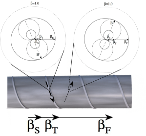
Figure 19.— Role of the phase polar diagram in a helical magnetic field jet model. We show a relativistic plasma jet (medium grey flow) in its rest frame, described by Model (b) (discussed in the text), and wrapped with one of its many helical magnetic field lines. At left the phase polar diagram in Figure 18b is rotated by the angle $-\alpha$ to align the dashed arrow with the helical field direction on the near side of the jet (left). The propagation speeds of the three MHD waves along the jet axis then can be directly read off the polar diagram ($\beta_{\mathrm{S}}=0.112$, $\beta_{\mathrm{T}}=0.241$, $\beta_{\mathrm{F}}=0.675$). For a uniform helical field one obtains the same results at any point (e.g., on the far side of the jet at right.)

However, there will be a longitudinal current that will cause the field strength and pitch angle to be functions of the radial coordinate $\varpi$. (See the cut-away view of a plasma rope in Figure 6.14 of Gurnett & Bhattacharjee (2005), for a simple view of the radial variations in B and $\alpha$.) But, there should be a cylindrical shell around the axis, covering a modest range of $\varpi$, in which the synchrotron emissivity into the direction of the observer is maximized. We assume that this shell is the dominant region and that the field strength and pitch angle there are the effective values that control the dynamics. (See Lyutikov, Pariev, & Gabuzda (2005) for a discussion of this point. Thus, if this is the case, then our dynamical analysis of the waves and a polarization analysis of the emission should result in similar magnetic pitch angle estimates for the magnetic field. A preliminary polarization analysis (using methods similar to those in Murphy, Cawthorne & Gabuzda (2013) and to be discussed in more detail in the next paper in this series) produces estimates of at least 60^∘- 70^∘for the pitch angle. This is in agreement with our result for the hot Model (b), which gives $\alpha\approx 67^{\circ}$.

7. Summary and Conclusions

The jet of BL Lac is highly variable and displays transverse patterns that propagate superluminally downstream on the ridge line. They are not ballistic, like water from a hose, but are constrained, like waves on a whip. The magnetic field is well-ordered with a strong transverse component that we assume is the toroidal part of a helical field. In Cohen et al. (2014) we assumed that the helical field provided support for fast- and slow-mode MHD waves whose compressions we see as the superluminal components. We here assume that the moving transverse patterns are Alfvén waves propagating on the longitudinal component of the magnetic field.

The full set of ridge lines is shown in Figure 2, and we show six examples of the Alfvén waves in Figures 7, 9, 10, 11, and 12. A movie (Figure 13) provides assistance in studying the motions.

The transverse wave activity died down in 2010 and the jet settled to a fixed position angle (P.A.), with a mild wiggle. This wiggle was not stationary, but appeared to oscillate transversely, with amplitude about 0.4 mas. This mild wiggle persisted through the remaining data period, up to 2013.0.

Although the transverse propagating Alfvén waves were greatly reduced in 2010-2013, the superluminal components, which we identified in Paper I as MHD sonic waves, continued roughly as before. Figure 2 in Paper I shows that during this period they continued with about the same frequency and speed as earlier. Furthermore, during the latter half of this period, from about 2011.4 to 2013.0, BL Lac was exceptionally active at shorter wavelengths (Raiteri et al., 2013), from 1 mm through gamma-rays. This general behavior can fit into our model. We have magnetosonic waves responsible for the superluminal components, and Alfvén waves responsible for the moving transverse patterns. These are independent MHD modes, and can be separately excited. We suspect, however, that the increase in short-wavelength activity during the same period as the reduction in Alfvén waves (2010–2013) is not a coincidence.

The velocity of the transverse waves was established by finding characteristic points on the ridge lines where the slope changes, as well as by visual inspection of the delayed superposition of the ridge lines. Three of the apparent velocities are near $\beta_{{\rm app}}\approx 5$, and one is much faster, with $\beta_{{\rm app}}\approx 13$. With $\theta=6^{\circ}$ and $\rm\Gamma_{beam}^{gal}=4.5$ the speeds in the galaxy frame are approximately $\rm\beta_{T}^{gal}=0.98-0.998$ and in the beam frame $\rm\beta_{T}^{beam}=0.25-0.82$.

An Alfvén wave displaces the jet in the transverse direction, and the observed motion can be converted into a transverse speed. For wave D, the largest wave we observed, the transverse speed, in the galaxy frame, is $\beta_{\mathrm{tr}}^{\mathrm{gal}}\sim 0.09$. This is a rough estimate but safely non-relativistic, and consistent with our assumption that the waves have low amplitude.

The timing and direction of some of the the waves are correlated with the P.A. of the recollimation shock (RCS), which swings over 25^∘ in an irregular fashion. It appears that the waves are excited by the swinging of the RCS. This is analogous to exciting a wave on a whip by shaking it. In Paper I (Figure 3) we saw that the ridge lines occupy a cylinder about 0.7 mas wide and 3 mas long, or 3 ly wide and 120 ly long when a deprojection factor of 10 is used. (See also Caproni, Abraham, & Monteiro (2012) Figure 1.) We now understand that this cylinder is formed by the transverse waves, whose axes generally are close to the source axis at $\rm P.A.\approx-166^{\circ}$. The width is set by the amplitude of the largest waves while the length is set by the general bend of the source to the SE.

We briefly describe the Alfvén waves, and provide a method for calculating physical quantities in the jet in terms of the measured wave speeds. We investigate two simple models of the system; in the first the plasma is cold and the sound speed $\beta_{\mathrm{s}}=0$. This gives results for the Lorentz factor and the pitch angle that are in moderate disagreement with results from observations. The second model uses a hot plasma with $\beta_{s}=0.3$, and assumes that the slow magnetosonic wave has apparent speed $\rm\beta_{app,S}=4$. This yields $\rm\Gamma_{beam}\approx 4.5$, pitch angle $\alpha\approx 67^{\circ}$, Alfvén speed $\rm\beta_{A}\sim 0.64$, and magnetosonic Mach number $\rm M_{ms}\approx 4.7$. This describes a plasma in which the helical magnetic field is strong with a dominant toroidal component.

In our model the Lorentz factor for the beam is approximately 4.5 and is smaller than the observed apparent speed of most of the transverse waves as well as the fast superluminal components discussed in Paper I. Another way to say this is that in most cases the pattern speed is greater than the beam speed. This comes about because the pattern traces a wave traveling downstream on the beam.

We conclude that the rapid movements of the transverse patterns in the jet of BL Lac can be described as Alfvén waves excited at the RCS and propagating downstream on the longitudinal component of a helical magnetic field. The jet can be described as a relativistic, rapidly shaken whip. We suggest that other similar sources be investigated with these ideas in mind.

References

- Belcher, Davis & Smith (1969) Belcher, J. W., Davis, L. Jr. & Smith, E. J. 1969, J. Geophys. Res., 74, 2302
- Blandford & Königl (1979) Blandford, R. D. & Königl, A. 1979, ApJ, 232, 34
- Britzen et al. (2010a) Britzen, S. et al 2010a, A&A, 515, A105
- Britzen et al. (2010b) Britzen, S. et al 2010b, A&A, 511, A57
- Caproni, Abraham, & Monteiro (2012) Caproni, A., Abraham, Z. & Monteiro, H. 2012, MNRAS, 428, 280
- Cohen et al. (2007) Cohen, M. H., Lister, M. L., Homan, D. C., et al. 2007, ApJ, 658, 232
- Cohen et al. (2014) Cohen, M. H. et al. 2014, ApJ, 787, 151 (Paper I)
- Edberg et al. (2010) Edberg, N. J. T. et al. 2010, J. Geophys. Res., 115, AO7203
- Fanaroff & Riley (1974) Fanaroff, B. L. & Riley, J. M. 1974, MNRAS, 167, 31
- Fermi (1949) Fermi, E. 1949, Physical Review, 75, 1169
- Gabuzda (1999) Gabuzda, D. C. 1999, New Astronomy Reviews, 43, 691
- Gabuzda, Murray & Cronin (2004) Gabuzda, D. C., Murray, É. & Cronin, P. J. 2004, MNRAS, 351, L89
- Gabuzda & Pushkarev (2001) Gabuzda, D. C. & Pushkarev, A. 2001, in ASP Conf. Ser. 250, Particles and Fields in Radio Galaxies, eds R. A. Liang & K. M. Blundell, 180
- Goldreich & Lynden-Bell (1969) Goldreich, P. & Lynden-Bell, D. 1969, ApJ, 156, 59
- Goldreich & Sridhar (1997) Goldreich, P., & Sridhar, S. 1997, ApJ, 438, 763
- Gurnett & Bhattacharjee (2005) Gurnett, D. A. & Bhattacharjee, A. 2005, “Introduction to Plasma Physics”, Cambridge, p199
- Gurnett & Bhattacharjee (2005) Gurnett, D. A. & Bhattacharjee, A. 2005, “Introduction to Plasma Physics”, Cambridge, p208
- Hardee, Walker & Gómez (2005) Hardee, P. E., Walker, R. C. & Gómez, J. L. 2005, ApJ, 620, 646
- Hovatta et al. (2009) Hovatta, T., Valtaoja, E., Tornikoski, M. & Lahteenmaki, A. 2009, A&A, 494, 527
- Hovatta et al. (2014) Hovatta, T. et al. 2014, AJ, 147, 143
- Hughes (2005) Hughes, P. A. 2005, ApJ, 621, 635
- Hughes Aller & Aller (1989a) Hughes, P. A., Aller, H. D. & Aller, M. F. 1989a, ApJ, 341, 54
- Hughes, Aller, & Aller (1989b) Hughes, P. A. Aller, H. D. & Aller, M. F. 1989b, ApJ, 341, 68
- Hughes, Aller, & Aller (1991) Hughes, P. A. Aller, H. D. & Aller, M. F. 1991, ApJ, 374, 57
- Jorstad et al. (2005) Jorstad, S. G. et al. 2005, AJ, 130, 1418
- Kellermann et al. (1998) Kellermann, K. I., Vermeulen, R. C., Zensus, J. A. & Cohen, M. H. 1998, AJ, 115, 1295
- Kovalev et al. (2008) Kovalev, Y. Y., Lobanov, A. P., Pushkarev, A. B. & Zensus, J. A. 2008, A&A, 483, 759
- Lind et al. (1989) Lind, K. R., Payne, D. G., Meier, D. L., & Blandford, R. D. 1989, ApJ, 344, 89
- Lister & Homan (2005) Lister, M. L. & Homan, D. C. 2005, AJ, 130, 1389
- Lister et al (2009) Lister, M. L., Cohen, M. H., Homan, D. C., et al. 2009, AJ, 138, 1874
- Lister et al (2013) Lister, M. L., Aller, M. F., Aller H. D., et al. 2013, AJ, 146, 120
- Lobanov & Zensus (2001) Lobanov, A. P. & Zensus, J. A. 2001, Science, 294, 128
- Lyutikov, Pariev, & Gabuzda (2005) Lyutikov, M., Pariev, V. I. & Gabuzda, D. C. 2005, MNRAS, 360, 869
- Marscher & Gear (1985) Marscher, A. P. & Gear, W. K. 1985, ApJ, 298, 114
- Marscher (2014) Marscher, A. P. 2014, ApJ, 780, 87
- McIntosh et al. (2011) McIntosh, S. W., de Pontieu, B., Carlsson, M., Hansteen, V., Boerner, P. & Goossens, M. 2011, Nature, 475, 477
- Meier (2012) Meier, D. L. “Black Hole Astrophysics: The Engine Paradigm”, Springer, 2012, 717
- Meier (2013) Meier, D. L. 2013 in “The Innermost Regions of Relativistic Jets and Their Magnetic Fields”, EPJ Web of Conferences, 61, 01001
- Mizuno, Hardee, & Nishikawa (2014) Mizuno, Y., Hardee, P. E. & Nishikawa, K.-I. 2014, ApJ, 784
- Nakamura & Meier (2004) Nakamura, M. & Meier, D. L. 2004, ApJ, 617, 123
- Nakamura & Meier (2014) Nakamura, M. & Meier, D. L. 2014, ApJ, 785, 152
- Murphy, Cawthorne & Gabuzda (2013) Murphy, E., Cawthorne, T. V. & Gabuzda, D. C. 2013, MNRAS, 430, 1504
- O’Sullivan & Gabuzda (2009) O’Sullivan, S. P. & Gabuzda, D. C. 2009a, MNRAS, 393, 429.
- Perucho et al. (2006) Perucho, M., Lobanov, A. P., Martí, J.-M., & Hardee, P. E. 2006, A&A, 456, 493
- Perucho et al (2012) Perucho, M., Kovalev, Y. Y., Lobanov, A. P., Hardee, P. E. & Agudo, I. 2012, ApJ, 749, 55
- Perucho (2013) Perucho, M. 2013, European Physical Journal Web of Conferences, 61, 2002
- Pushkarev et al. (2012) Pushkarev, A. B. et al. 2012, A&A, 545, A113
- Raiteri et al. (2013) Raiteri, C. M. et al. 2013, MNRAS, 436, 1530