Distinguishing Cause from Correlation in Tokamak Experiments to Trigger Edge Localised Plasma Instabilities

Abstract

The generic question is considered: How can we determine the probability of an otherwise quasi-random event, having been triggered by an external influence? A specific problem is the quantification of the success of techniques to trigger, and hence control, edge-localised plasma instabilities (ELMs) in magnetically confined fusion (MCF) experiments. The development of such techniques is essential to ensure tolerable heat loads on components in large MCF fusion devices, and is necessary for their development into economically successful power plants. Bayesian probability theory is used to rigorously formulate the problem and to provide a formal solution. Accurate but pragmatic methods are developed to estimate triggering probabilities, and are illustrated with experimental data. These allow results from experiments to be quantitatively assessed, and rigorously quantified conclusions to be formed. Example applications include assessing whether triggering of ELMs is a statistical or deterministic process, and the establishment of thresholds to ensure that ELMs are reliably triggered.

I Introduction

Presently the most successful high-performance nuclear fusion experiments use a toroidal magnetic field to confine the plasma in a tokamak Wesson . Unfortunately the most highly confined of these plasmas are susceptible to edge-localised instabilities (“ELMs”) Zohm , that eject particles and energy onto the plasma-facing components. In future power-plant scale devices, the size of the ELMs must be limited to avoid components being damaged. One proposal is to deliberately and rapidly trigger ELMs, with the hope of having a larger number of smaller ELMs. A method that has been found successful at triggering ELMs is to apply a rapidly increasing radial magnetic field to the plasma, that “kicks” the plasma vertically to trigger ELMs Degeling ; Lang ; Liang ; LangPacing . To understand and optimise the method it is necessary to explore the threshold between when the kicks trigger ELMs, and when they simply perturb the plasma. For example figure 1 shows a scan of kick sizes, with a systematic variation of the amplitude and duration of the voltage applied to coils that produce the radial magnetic field that can trigger the ELMs. For these situations it is necessary to be able to quantify the success by which ELMs are triggered, so as to better understand physically what is triggering the ELM, and practically, what is required to successfully do so. A complication is that ELMs occur regularly without kicks, so how can we determine whether an ELM is due to a kick or is naturally occurring? A major step towards this is to understand the time-scales over which the kick influences the plasma most strongly. This then determines a narrower time window when a kick is able to trigger an ELM, but it does not rule out the possibility that some ELMs occur naturally within that time window also. Correctly accounting for this possibility is a purpose of this paper. In the next section we outline how Bayesian probability theory can be used to formulate a general solution to this problem. The generic problem however is much broader - for example, how can you tell if the increase in insurance claims due to lightning strikes are due to global warming or statistical chance? It might be possible to adapt some of the methods here to those broader questions. The following sections explore how the solution can be applied to the specific question of determining the success of “kick-triggering” experiments.

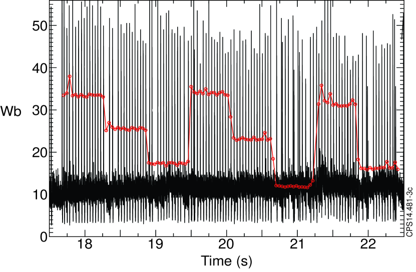
Figure 1: JET plasma 83440. The measured Volt seconds (Wb) of each kick is plotted (red circles) versus the time in seconds during the pulse, with the strong Be II light emissions due to ELMs superimposed (not to scale). For kicks with large amplitude in Wb, ELMs appear to be clearly synchronised with the kicks, but for small kicks such as those between 20.6s and 21.4s their influence is much less clear.

II Formulation and formal solution of the problem

Bayesian probability theory starts from some simple but reasonable requirements about a theory of probability, and shows how the usual laws of probability theory can be derived from them Jaynes , such as the basic product rule,

$$P(A,B|C)=P(A|B,C)P(B|C)=P(B|A,C)P(A|C)$$ (1)

and the basic sum rule,

$$P(A|C)+P(\bar{A}|C)=1$$ (2)

where $P(A,B|C)$ reads as the probability of $A$ and $B$ being simultaneously true given that $C$ is true, and $P(A|B,C)$ reads as the probability of $A$ being true given that $B$ and $C$ are true, and $\bar{A}$ is used to denote the negation of $A$ (i.e. “not $A$”). These relations can be used to formulate a variety of mathematical expressions that relate the probability of events Jaynes . One useful expression that is derived in the appendix for convenience is,

$$P(A|C)=P(A|B,C)P(B|C)+P(A|\bar{B},C)P(\bar{B}|C)$$ (3)

In the context of our subsequent discussion this will be used to obtain the probability of the event $A$ occurring at time $t$, in terms of the probability of event $A$ occurring at time $t$ given that action $B$ has (or has not) triggered the event, with $C$ determining the time at which the triggering is attempted. Specifically we consider the probability density of observing the next ELM at time $t$ to $t+dt$ after a “vertical kick” starts to influence the plasma at $t=\tau_{m}$, with,

$$P(t|\tau_{m})=P(t|K,\tau_{m})P(K|\tau_{m})+P(t|\bar{K},\tau_{m})P(\bar{K}|\tau_{m})$$ (4)

where $P(t|\tau_{m})$ is the probability density of observing an ELM at time $t$ after a (vertical) kick starts to influence the plasma at time $\tau_{m}$, $P(t|K,\tau_{m})$ is the probability density of an ELM at time $t$ after $\tau_{m}$ given that a kick at has successfully triggered an ELM, and $P(t|\bar{K},\tau_{m})$ is the probability density of an ELM at time $t$ after $\tau_{m}$ if a kick has failed to trigger an ELM. $P(K|\tau_{m})$ is the probability of a kick successfully triggering an ELM and $P(\bar{K}|\tau_{m})$ is the probability of a kick not triggering an ELM, given that the kick starts to influence the plasma at time $\tau_{m}$. Because of (2), $P(\bar{K}|\tau_{m})=1-P(K|\tau_{m})$, and we have,

$$P(t|\tau_{m})=P(t|K,\tau_{m})P(K|\tau_{m})+P(t|\bar{K},\tau_{m})(1-P(K|\tau_{m}))$$ (5)

This equation is exact, and can be developed in various ways. The aim is to construct a mathematical expression whose terms can be accurately estimated from the available experimental data, allowing $P(K|\tau_{m})$ to be determined. Here (5) will be used to formalise the idea that triggered ELMs will appear in a short time interval after a kick, using the information to rigorously define the probability of an ELM having been triggered. Crucially, this is done in a way that allows the possibility that some of the observed ELMs will have occurred naturally, the resulting estimates quantitatively account for this.

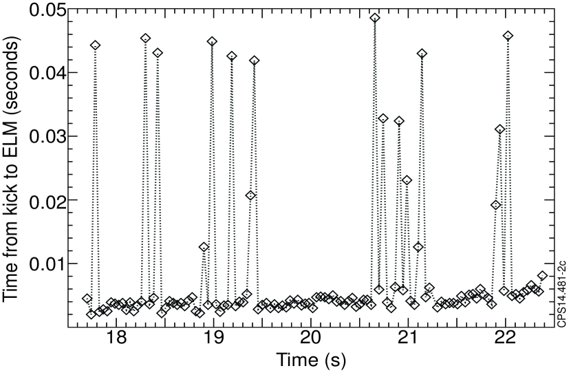
Figure 2: JET plasma 83440. The time from the start of a kick to the next ELM is plotted versus time during the plasma pulse. Due to the limited kick duration and the time for the kicked magnetic field to diffuse through the plasma, kicks can only influence the plasma for of order 1-8 ms after they start. Most of the ELMs bunched within this time interval will have been triggered by a kick, although some may have occurred naturally.

Some background. Following a “kick” in the JET tokamak, there is a time period of order $1$-$1.5$ milliseconds before the kick’s magnetic field starts to strongly interact with the plasma, and another time period proportional to the kick’s duration, before the kick reaches its maximum strength. The time delay is due to the time needed for the magnetic field that the control coils are trying to produce, to diffuse through JET’s metal vacuum vessel and other conducting components. By observing ELMs that are clearly triggered and paced at the kick-frequency, it appears that triggered ELMs occur approximately within $\tau_{m}$ to $\tau_{m}+\Delta\tau$, where $\Delta\tau$ is the kick’s duration. For example see figure 2, whose results are consistent with a resistive diffusion of the “kicked” magnetic field through JET’s metal vacuum vessel over a 1.0-1.5 ms timescale, and ELMs being triggered after the magnetic perturbation has grown towards its maximum value over a timescale of 1.5-4.5ms depending on the kick’s duration and amplitude. However, we cannot infer the kick success simply by counting the fraction of ELMs that occur in this time period after a kick, because a fraction of those will be expected to occur in that time interval naturally. Eq. 5 accounts for this through the term $P(t|\bar{K},\tau_{m})P(\bar{K}|\tau_{m})$, the probability of observing ELMs at a time $t$ since a kick, given that the ELM is not triggered. Formally all of this can be achieved by integrating both sides of (5) from $\tau_{m}$ to $\tau_{m}+\Delta\tau$, with respect to $t$. Then after integration we get,

$$P_{\Delta\tau}=P(K)+P_{\bar{K}}\left(1-P(K)\right)$$ (6)

where $P_{\Delta\tau}\equiv\int_{\tau_{m}}^{\tau_{m}+\Delta\tau}P(t)dt$, $\int_{\tau_{m}}^{\tau_{m}+\Delta\tau}P(t|K)dt=1$ by the definition that these kicks will successfully trigger ELMs, and $P_{\bar{K}}\equiv\int_{\tau_{m}}^{\tau_{m}+\Delta\tau}P(t|\bar{K})dt$ is the probability of ELMs occurring naturally and being observed within $\tau_{m}$ to $\tau_{m}+\Delta\tau$ without having been triggered by kicks. Consequently,

$$P(K)=\frac{P_{\Delta\tau}-P_{\bar{K}}}{1-P_{\bar{K}}}$$ (7)

$P_{\Delta\tau}$ and $P_{\bar{K}}$ both depend on $\Delta\tau$ and $\tau_{m}$, although for reasonably large numbers of kicks we will find that $P_{\bar{K}}$ (and consequently $P_{\Delta\tau}$), are approximately independent of $\tau_{m}$. Notice that if we had ignored naturally occurring ELMs, with $P_{\bar{K}}=0$, we would simply have $P(K)=P_{\Delta\tau}$, or in other words, we would estimate the probability of a kick successfully triggering an ELM simply as the probability of observing an ELM in the “kick-triggered” time interval. If $P_{\bar{K}}$ is sufficiently small then the estimates of $P(K)=P_{\Delta\tau}$ and (7) will be similar. Also if $P_{\bar{K}}$ is small, then,

$$P(K)=P_{\Delta\tau}-P_{\bar{K}}\left(1-P_{\Delta\tau}\right)+O\left(P_{\bar{K}}^{2}\right)$$ (8)

which is useful for obtaining simple leading-order error estimates as the sum of errors in $P_{\Delta\tau}$ and $P_{\bar{K}}$, which are easy to calculate and record. For kick-triggering studies, $P_{\bar{K}}$ is usually small. $P_{\Delta\tau}$ can be estimated from the kick-ELM data by counting the number of ELMs that occur naturally within the set of time intervals $\tau_{m}$ to $\tau_{m}+\Delta\tau$; this will be considered in a later section. $P_{\bar{K}}$ can be estimated from equivalent ELMing plasma data without kicks, which we discuss next.

III Estimating $P_{\bar{K}}$

Next we consider how to estimate $P_{\bar{K}}$ from ELM time data that does not have kicks or other triggering mechanisms. Firstly we calculate the probability of an ELM being observed in a time interval $\tau_{m}$ to $\tau_{m}+\Delta\tau$, finding a simple estimate for the limit where $\tau_{m}\sim n\bar{t}$ has $n\gg 1$. This is a useful approximation, so we explore when it is reasonable, and test the estimate by calculating the number of ELMs that we would expect to occur naturally in the time intervals ($\tau_{m}$,$\tau_{m}+\Delta\tau$) that we might incorrectly think are “triggered” ELMs, and compare this estimate with observations from experimental data.

The probability of observing the $n$th ELM in ($\tau_{m}$,$\tau_{m}+\tau$), is,

$$\int_{\tau_{m}}^{\tau_{m}+\tau}p(x|n)dx$$ (9)

where $x=\sum_{i=1}^{n}t_{i}$, and $t_{i}$ are the waiting times between the $(i-1)$th and $i$th ELM. The probability of any ELM being in ($\tau_{m}$, $\tau_{m}+\tau$), is,

$$P_{\bar{K}}(\tau_{m})=\sum_{n=1}^{\infty}\int_{\tau_{m}}^{\tau_{m}+\tau}p(x|n)dx$$ (10)

for the present we have decided to explicitly emphasise the dependence of $P_{\bar{K}}$ on $\tau_{m}$ by writing $P_{\bar{K}}(\tau_{m})$. As is outlined in 7.16 of Jaynes Jaynes , $p(x|n)$ can be written as,

$$p(x|n)=\frac{1}{2\pi}\int_{-\infty}^{\infty}\psi(\alpha)^{n}e^{-i\alpha x}d\alpha$$ (11)

with,

$$\psi(\alpha)=\int_{-\infty}^{\infty}P(t)e^{i\alpha t}dt$$ (12)

where $P(t)$ is the ELM waiting time pdf, that gives the probability of observing an ELM in time $t$ to $t+dt$ as $P(t)dt$. For many situations $P(t)$ can be reasonably approximated by a Gaussian WebsterDendy2013 , and for those cases we exactly have,

$$p(x|n)=\frac{1}{\sqrt{2\pi n\sigma^{2}}}\exp\left(-\frac{(x-n\bar{t})^{2}}{2n\sigma^{2}}\right)$$ (13)

where $\bar{t}$ is the average ELM waiting time and $\sigma$ is the ELM waiting times’ standard deviation. These two quantities $\bar{t}$ and $\sigma$ can be estimated from the ELM time data with an error of order $1/\sqrt{M}$, where $M$ is the total number of observed ELMs Sivia . Equation (13) is exact Jaynes whenever $P(t)$ is a Gaussian, however if $n\gg 1$ then with only a small number of exceptions Jaynes , the Central Limit Theorem ensures that (13) remains true independent of the specific form of ELM waiting time pdf Jaynes . Using (10) and (13) the probability of an ELM in time $\tau_{m}$ to $\tau_{m}+\tau$ is,

$$P_{\bar{K}}(\tau_{m})=\sum_{n=1}^{\infty}\int_{\tau_{m}}^{\tau_{m}+\tau}\frac{dx}{\sqrt{2\pi n\sigma^{2}}}\exp\left(-\frac{(x-n\bar{t})^{2}}{2n\sigma^{2}}\right)$$ (14)

For $n\bar{t}\gg\bar{t}$ ($n\gg 1$) , the sum can be approximated by an integral, with $y=n\bar{t}$ and $dy=\bar{t}$, giving,

$$P_{\bar{K}}=\int_{0}^{\infty}\frac{dy}{\bar{t}}\int_{\tau_{m}}^{\tau_{m}+\tau}\frac{dx}{\sqrt{2\pi y(\sigma^{2}/\bar{t})}}\exp\left(-\frac{(x-y)^{2}}{2y(\sigma^{2}/\bar{t})}\right)$$ (15)

where the dependence of $P_{\bar{K}}$ on $\tau_{m}$ has been removed for reasons that will be explained shortly. Changing variables, with $x=\hat{x}\sigma^{2}/\bar{t}$ and $y=v^{2}\sigma^{2}/\bar{t}$, so that $dy/\sqrt{y}=2dv(\sigma^{2}/\bar{t})$, and exchanging the order of integration, gives,

$$P_{\bar{K}}=\frac{1}{\bar{t}}\int_{\tau_{m}(\sigma^{2}/\bar{t})}^{(\tau_{m}+\tau)(\sigma^{2}/\bar{t})}d\hat{x}\left(\frac{\sigma^{2}}{\bar{t}}\right)\frac{1}{\sqrt{2\pi}}\int_{0}^{\infty}dv\exp\left(\frac{(x-v^{2})^{2}}{2v^{2}}\right)$$ (16)

Using the integral Schulman ,

$$\int_{0}^{\infty}dx\exp\left(-ax^{2}-\frac{b}{x^{2}}\right)=\sqrt{\frac{\pi}{4a}}\exp\left(-2\sqrt{ab}\right)$$ (17)

it can easily be shown that,

$$\int_{0}^{\infty}dv\exp\left(-\frac{(\hat{x}-v^{2})^{2}}{2v^{2}}\right)=\sqrt{\frac{\pi}{2}}$$ (18)

a surprising result, because like a normalised probability distribution with a parameter $\hat{x}$, the result is independent of $\hat{x}$. Consequently, doing the final integral over $\hat{x}$ and cancelling terms, we get,

$$P_{\bar{K}}=\frac{\Delta\tau}{\bar{t}}$$ (19)

A surprising and disappointing aspect of (19) is that $\tau_{m}$ does not appear, and the influence of correlations when $\tau_{m}\simeq\bar{t}$ for example, are not captured by the calculation. The only approximation that is always present enters subtly, through the need of $n\gg 1$ for the sum to be accurately approximated by an integral. The approximation $n\gg 1$ removes the information about the discrete nature of ELMs and consequently is unable to describe the influence of correlations between $\tau_{m}$ and $\bar{t}$. Consider the example with $\tau_{m}$ small. Then (9) could be accurately approximated by keeping only the first few terms in the sum over $n$, and the approximation of (15) would be poor. The influence of correlations between the natural ELM frequency and the kick frequency is discussed in the Appendix, where it finds that provided $\Delta\tau/\sigma$ is reasonably small, where $\sigma$ is the standard deviation in the natural ELM period, then any coherence between the natural ELMs and kick frequency will be rapidly lost within the first one or possibly two ELMs. Another caveat is that if $P(t)$ is non-Gaussian, then $n\gg 1$ is required for the central limit theorem to ensure that $p(x|n)$ will tend to (13); but occasionally for some distributions even if $n\gg 1$ the rate of convergence can be slow and the estimates less good than expected. In summary, for small $\tau_{m}/\bar{t}$, for which $n\sim 1$ is most relevant, then in principle equations (9), (11), and (12) must be used; but despite the caveats mentioned above, provided $\tau_{m}/\bar{t}\gg 1$ and $\Delta\tau/\sigma$ are reasonably small then (15) and (19) should in most cases provide an accurate approximation.

Estimates for $\bar{t}$ and $\sigma$ must be found from equivalent ELM data for natural (untriggered) ELMs. They can be estimated from a set of $M$ ELM waiting times $\{t_{i}\}$, of $\bar{t}\simeq\frac{1}{M}\sum_{i=1}^{M}t_{i}$ and $\sigma^{2}\simeq\frac{1}{M-1}\sum_{i=1}^{M}(t_{i}-\bar{t})^{2}$ both of which have errors of order $1/\sqrt{M}$ Sivia . Ideally there will be plenty of data for natural ELMs, so that $M\gg 1$, and we can neglect the errors in $\bar{t}$ and $\sigma$ compared with the other errors in (23). Otherwise the leading order errors give,

$$P_{\bar{K}}\simeq\frac{\Delta\tau}{\bar{t}}\left(1\pm\frac{\sigma}{\bar{t}\sqrt{M}}\right)$$ (20)

with the error estimated from $\bar{t}\simeq(1/M)\sum_{i=1}^{M}t_{i}\pm\sigma/\sqrt{M}$. The greatest source of systematic error is likely to be through unintended changes to the plasma’s properties between pulses, leading to incorrect estimates for $\bar{t}$ and $\sigma$. This risk can be reduced by using a reference pulse from the same session, or a reference phase from within a pulse, although longer pulses will give greater statistical accuracy. In practice $P_{\bar{K}}$ is comparatively small, and unless the number of kicks are much larger than the $\sim$15 in the example considered here, then the errors are dominated by those in $P_{\Delta\tau}$ that are statistical in origin and can only be reduced by increasing the number of kicks in the study.

We can test Eq. 19 by calculating the number of natural (untriggered) ELMs we would expect to observe in the “kick-triggered” time intervals, and compare this with the number that are observed in equivalent time intervals of experimental data (without kicks). Assuming that (19) is a reasonable approximation for $P_{\bar{K}}$, as it very often will be, then we can estimate $N_{\bar{K}}$ as follows. The probability of observing an unordered sequence of $N_{K}$ time intervals ($\tau_{1}$, $\tau_{1}+\tau$), ($\tau_{2}$, $\tau_{2}+\tau$), … , ($\tau_{N_{K}}$, $\tau_{N_{K}}+\tau$), with $N_{\bar{K}}$ ELMs spread among them is given by,

$$P(N_{\bar{K}},N_{K})=\left(\begin{array}[]{c}N_{K}\\ N_{\bar{K}}\end{array}\right)\left(P_{\bar{K}}\right)^{N_{\bar{K}}}\left(1-P_{\bar{K}}\right)^{N_{K}-N_{\bar{K}}}$$ (21)

i.e. the Binomial distribution (because the order in which the $N_{\bar{K}}$ natural ELMs coincide with an interval $\tau_{i}$ to $\tau_{i}+\Delta\tau$ is not important). Consequently the expected number of (untriggered) ELMs to be observed by chance in the “triggered ELMs” time interval can be calculated from $\langle N_{\bar{K}}\rangle=\sum_{N_{\bar{K}=1}}^{N_{K}}N_{\bar{K}}P(N_{\bar{K}},N_{K})$, and is found using (19) for $P_{\bar{K}}$ to be,

$$\langle N_{\bar{K}}\rangle=N_{K}\frac{\Delta\tau}{\bar{t}}$$ (22)

The standard deviation is $\sqrt{\langle N_{\bar{K}}^{2}\rangle-\langle N_{\bar{K}}\rangle^{2}}=\sqrt{N_{K}\frac{\Delta\tau}{\bar{t}}\left(1-\frac{\Delta\tau}{\bar{t}}\right)}$, which allows an estimate for the error in (22). Therefore taking $N_{\bar{K}}\simeq\langle N_{\bar{K}}\rangle$, we obtain an estimate of,

$$N_{\bar{K}}\simeq N_{K}\frac{\Delta\tau}{\bar{t}}\pm\sqrt{N_{K}\frac{\Delta\tau}{\bar{t}}}\sqrt{1-\frac{\Delta\tau}{\bar{t}}}$$ (23)

Eq. 23 allows us to estimate $N_{\bar{K}}$, given the number of kicks $N_{K}$, and a reference phase of normal ELMs from which the ELMs’ average waiting time $\bar{t}$ and standard deviation $\sigma$ can be estimated.

To test the above Eq. 23, we count the number of ELMs within time intervals of $n\times$(0.02) to $n\times$(0.02)+0.004 seconds, with $n$= 0,1,2, … , during the time period of 9-13.5 seconds of ten equivalent JET plasmas that do not have kicks. Details of the pulses are in Brez , we consider the subset of: 83630, 83629, 83628, 83627, 83626, 83625, 83624, 83640, 83641, and 83642, for which the average ELM waiting time across all pulses was $\bar{t}=0.030$ seconds. Figure 3 plots the number of ELMs that are counted in the time intervals that would usually be presumed to be “kick-triggered”, divided by the number of “kick-triggered” time intervals (estimated as the time divided by the period between the intervals), along with our estimate for $N_{\bar{K}}/N_{K}$ using Eq. 23. The agreement is surprisingly good. If the results were Gaussianly distributed then we would expect approximately 68% of the data sets to be within one standard deviation, indicated on the plots by the dashed lines. The results are reassuringly consistent with this.

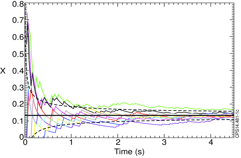
Figure 3: Comparison between calculated estimates for $N_{\bar{K}}$, and observed from experimental data. For ten equivalent JET plasmas, the number of ELMs are counted that occur by chance within the set of intervals $\tau_{m}$ to $\tau_{m}+\Delta\tau$, that if kicks were present would be presumed to be kick-triggered. Theoretical lines are: the estimated average (thick black line), the average $\pm$ the standard deviation (dashed black lines). Assuming the data is Gaussianly distribution then we would expect 68% of results to be within the dashed lines. The results are reassuringly consistent with this.

IV Estimating $P_{\Delta\tau}$

The estimation of $P_{\Delta\tau}$ given the observation of $m$ ELMs in $n$ “kick-triggered” time intervals, is a classic and well-known problem in Bayesian probability theory that we will briefly review next. The probability of observing $m$ successes in $n$ trials, with a probability $p$ of a success at each trial, is given by the binomial distribution,

$$P(m,n|p)=\left(\begin{array}[]{c}n\\ m\end{array}\right)p^{m}(1-p)^{n-m}$$ (24)

Bayes theorem gives Sivia ; Jaynes ,

$$P(p|m,n)=\frac{P(m,n|p)P(p)}{\int_{0}^{1}P(m,n|p)P(p)dp}$$ (25)

which allows us to obtain a probability distribution for $p$ given the observed $m$ successes from $n$ trials, and a suitable prior distribution $P(p)$. Present models for ELMs have ELMs being triggered once a threshold of pressure gradient or current is exceeded WebsterRev . If we regard kick-triggering in a similar way, with a probability of success that rapidly steps between zero and one - either a kick is strong enough to trigger an ELM or it is not, then we might follow the reasoning of Jaynes (pages 382-386 of Ref. Jaynes ), that leads to the “Haldane” prior $P(p)$ with,

$$P(p)=\frac{C}{p(1-p)}$$ (26)

with $C$ a constant. Using this prior in (25) along with (24) for $P(m,n|p)$, we get (after doing the integral in the denominator) Jaynes ,

$$P(p|m,n)dp=\frac{(n-1)!}{(m-1)!(n-m-1)!}p^{m-1}(1-p)^{n-m-1}dp$$ (27)

This gives an expected value for $p$ of,

$$\langle p\rangle=\frac{m}{n}$$ (28)

with a standard deviation $\sigma$ of,

$$\sigma=\sqrt{\frac{m(n-m)}{n^{2}(n+1)}}$$ (29)

Alternately, we might regard kick-triggering as a statistical process as in WebsterDendy2013 , with a success probability that increases gradually with the size of the kick. Then it would seem reasonable to take a uniform prior, with $P(p)$ a constant. With this assumption we get,

$$P(p|m,n)dp=\frac{(n+1)!}{m!(n-m)!}p^{m}(1-p)^{n-m}dp$$ (30)

This gives an expected value for $p$ of,

$$\langle p\rangle=\frac{m+1}{n+2}$$ (31)

with a standard deviation $\sigma$ of,

$$\sigma=\sqrt{\frac{(m+1)(n-m+1)}{(n+2)^{2}(n+3)}}$$ (32)

Whichever prior we regard as being most reasonable, we can estimate $P_{\Delta\tau}$ from the $N$ ELMs observed during the total of $N_{K}$ kicked time intervals, as,

$$P_{\Delta\tau}\simeq\langle p\rangle\pm\sigma$$ (33)

with $\langle p\rangle$ and $\sigma$ estimated from either 28 and 29, or 31 and 32. We will evaluate $P_{\Delta\tau}$ with both priors to provide examples of how the results can become modified.

Equations 7, 20, and 33 allow us to rigorously estimate the probability of kicks triggering ELMs, given the number of kicks $N_{K}$, a suitable estimate for $\tau_{m}$ and $\Delta\tau$, the observed number of ELMs $N$ in the intervals $\tau_{m}$ to $\tau_{m}+\Delta\tau$, and an equivalent phase of plasma with natural (unkicked) ELMs from which to estimate $N_{\bar{K}}$ from (20).

V Examples: Quantifying kick-triggering success

A kick consists of a step in the voltage that is applied to the vertical control coils, that has a duration in time and an amplitude KickRef . In a recent JET experiment (pulse 83440), the duration and amplitude of the kick was deliberately varied to explore how kick-triggering success depended on them. To analyse the kick-triggering probability it is necessary to explore a bit more of the physics involved in a vertical kick. The diffusion time of JET’s vacuum vessel is of order 1.3ms, so a kick of duration $\tau_{kick}$ has negligible influence on the plasma for 1.3ms, has a maximum perturbation over $\tau_{kick}$ to $\tau_{kick}+1.3$ms, and falls to less than half of its value in of order $2\times\tau_{kick}$. Based on past experience, ELMs in JET are not expected to be triggered with kicks of less than 10Wb (10 Volt seconds), so it seems safe to assume that a kick cannot modify plasma stability until it has produced at least 5Wb. After $\sim$1.3ms the kick’s constant voltage produces a perturbation to the radial magnetic field that grows approximately linearly with time, at least for kick durations of less than 4-5ms or so. So for a kick with voltage $V_{kick}$ it seems reasonable to define a minimum time $\tau_{m}$ for which $(\tau_{m}-1.3)V_{kick}=5$, i.e. $\tau_{m}=5/V_{kick}+1.3$, below which the kick has negligible influence. If we take $2\tau_{kick}$ as an upper time limit over which the kick significantly perturbs the plasma, then $\Delta\tau=2\tau_{kick}-5/V_{kick}-1.3$.

JET plasma pulse 83440 was based on the plasma in pulse 82630 over the period 18.5-20s, that was extended in 83440 to allow kicks to be tested over an extended pulse duration. During the 18.5-20s period in 82630 there were $M=24$ ELMs, with an average period $\bar{t}=0.059$ and standard deviation of $\sigma=0.011$. This gives $\sigma/\bar{t}\sqrt{M}=0.038$. Within the pulse 83440 the kick amplitude and duration are varied, as shown in figure 1, with results as in figure 2, and as recorded in table 1. The different kick durations lead to different values of $\Delta\tau$ that are also recorded in table 1, along with the number of kicks in each set $N_{K}$, the number of ELMs that occur in the time interval $\tau_{m}$ to $\tau_{m}+\Delta\tau$, and the values estimated from that data for $P_{\bar{K}}$, $P_{\Delta\tau}$, $P(K)$, and their errors. The quoted error for $P(K)$ is the largest of the upper and lower errors as calculated using the estimates for $P_{\Delta\tau}$ and $P_{\bar{K}}$. The Haldane prior biases the results towards kicks being one of either successful or unsuccessful, and consequently because estimates for $P(K)$ are all greater than $0.5$, the Haldane prior gives higher kick-triggering probabilities than the uniform prior. Intuitively, the author feels more comfortable with the more conservative, lower estimates for $P(K)$ that are obtained with a uniform prior, although most present models for ELM triggering favour a clear threshold for an ELM being triggered, or not. Independent of the choice of prior, from a physical point of view the results are surprising, because they indicate that kicks with quite small amplitude can still trigger ELMs if their duration is long enough. This has never previously been demonstrated, and can only be claimed with confidence because of the analysis presented here. When applied to larger data sets, a similar analysis will allow the quantitative assessment of how kick-triggering of ELMs depends on the kick properties such as its amplitude, duration, total Webers (Volt seconds), and maximum magnetic field perturbation. This will help us to understand how kicks trigger ELMs, and to optimise the kick properties for triggering ELMs with the “softest” possible kick with lowest voltage for example.

Kick Properties of JET pulse 83440
$V_{kick}$ (kV)	12	9	6	9	6	3	6	3
$\tau_{kick}$ (ms)	2.5	2.5	2.5	3.3	3.3	3.3	4.5	4.5
$\Delta\tau$ (ms)	3.3	3.1	2.9	4.7	4.5	3.6	6.9	6.0
$P_{\bar{K}}$	0.056 $\pm$ 0.002	0.053 $\pm$ 0.002	0.049 $\pm$ 0.002	0.080 $\pm$ 0.003	0.076 $\pm$ 0.003	0.062 $\pm$ 0.002	0.116 $\pm$ 0.004	0.102 $\pm$ 0.004
$N_{K}$	15	15	15	14	14	14	14	14
$N$	14	13	9	14	14	9	14	11
With uniform prior for $P(p)$
$P_{\Delta\tau}$	0.882 $\pm$ 0.076	0.824 $\pm$ 0.090	0.588 $\pm$ 0.116	0.938 $\pm$ 0.059	0.938 $\pm$ 0.059	0.625 $\pm$ 0.117	0.938 $\pm$ 0.059	0.750 $\pm$ 0.105
$P(K)$	0.88 $\pm$ 0.09	0.81 $\pm$ 0.10	0.57 $\pm$ 0.12	0.93 $\pm$ 0.07	0.93 $\pm$ 0.07	0.60 $\pm$ 0.13	0.93 $\pm$ 0.07	0.72 $\pm$ 0.12
With Haldane prior $P(p)=1/p(1-p)$
$P_{\Delta\tau}$	0.933 $\pm$ 0.062	0.867 $\pm$ 0.085	0.600 $\pm$ 0.122	1.000 $\pm$ 0.000	1.000 $\pm$ 0.000	0.643 $\pm$ 0.124	1.000 $\pm$ 0.000	0.786 $\pm$ 0.106
$P(K)$	0.93 $\pm$ 0.06	0.86 $\pm$ 0.09	0.58 $\pm$ 0.12	1.0 $\pm$ 0.00	1.00 $\pm$ 0.00	0.62 $\pm$ 0.12	1.00 $\pm$ 0.00	0.76 $\pm$ 0.11

Table 1: The table summarises the kick properties and successes for JET pulse 83440, recording the voltage $V_{kick}$ and duration $\tau_{kick}$ of the kick. $V_{kick}$ and $\tau_{kick}$ determine the duration $\Delta\tau$ over which the kick influences the plasma, allowing an estimate for $P_{\bar{K}}$ to be calculated. The number of kicks and the number of ELMs within a time interval $\Delta\tau$ allows an estimate for $P_{\Delta\tau}$ to be calculated, and subsequently also for $P(K)$ the probability of the kick triggering an ELM. Estimates are calculated with a uniform prior $P(p)$, and with the Haldane prior $P(p)=1/p(1-p)$.

VI What can we learn about ELMs, and how to mitigate them?

The previous section mentioned some of the opportunities that the techniques in this paper offer, the next few paragraphs discuss some of the possibilities more fully.

VI.1 Is ELM occurrence a deterministic process? Or is it better regarded as statistical?

Even steady-state tokamak plasmas are turbulent, and have continuously changing properties that are often best described in a statistical way. In contrast, ideal MHD models for ELM instabilities have ELMs being triggered after a specific threshold is exceeded in edge pressure gradient or current WebsterRev ; Groebner . A question is, is it more helpful to regard ELMs as a deterministic or statistical process? There is growing evidence that a statistical description of ELMs might be required. For example, WebsterDendy2013 shows many examples where the times between ELMs can be described by a Weibull probability distribution. This is consistent with the likelihood of observing an ELM in the next fraction of time, increasing with the time since the previous ELM, so it has elements of both a statistical and a deterministic model. More strikingly, in a set of 120 identical JET plasma pulses where the ELM energies were determined from the estimated losses of plasma thermal energy, it was found that the majority of ELM energies were statistically equivalent and independent of both the time since the previous ELM and the size of the previous ELM SJWebster . This seems contrary to the usual picture of ELMs, where we would expect the time to the next ELM to be determined by the time for the plasma’s edge properties to be restored to their pre-ELM values, and for this to be longer following a larger ELM. We might also have expected the ELM size to increase with time since the previous ELM, but beyond an initial recovery period of about 20 milliseconds the ELM energies were found to be independent of the time since the previous ELM SJWebster .

In principle vertical kicks provide an opportunity to test these pictures, by establishing whether there is a fixed threshold beyond which ELMs will be triggered and below which they cannot, or whether there is a smoothly continuous increase in the probability of triggering an ELM as the kick size is increased. In practice this study was not previously possible, because although it was clear when all ELMs are being triggered by kicks, when triggering is partially successful it is not possible to determine whether any particular ELM has been triggered or is naturally occurring, and there was no method to calculate the probability of ELMs having been triggered. This situation has now changed. Consider the example described in Table 1, of a 2T 2MA JET pulse in an otherwise steady-state H-mode with 10.2MW of neutral beam heating and 7.5$\times$10²²s^-1 of Deuterium gas fuelling. As the kick duration is reduced, with the kick voltage kept constant, the probability of a kick triggering an ELM falls gradually. For example, with a uniform prior for $P(p)$: $V_{kick}$=9 and $P(K)$ falls from 0.93 ($\tau_{kick}$=3.3ms) to 0.81 ($\tau_{kick}$=2.5ms), $V_{kick}$=6 and $P(K)$ falls from 0.93 ($\tau_{kick}$=3.3ms) to 0.57 ($\tau_{kick}$=2.5ms), $V_{kick}$=3 and $P(K)$ falls from 0.72 ($\tau_{kick}$=4.5ms) to 0.60 ($\tau_{kick}$=3.3ms); in none of these cases does $P(K)$ drop sharply toward zero. Similar conclusions are reached if we use the Haldane prior. Therefore for this case it appears that there is not a sharp threshold between whether an ELM is successfully triggered or not, but a gradual change in the probability of a kick being successful. Systematic experiments should be able to determine whether kick-triggering of ELMs should be regarded as a statistical process, and the circumstances for which this is the case, or not.

VI.2 What are the thresholds for kicks to trigger ELMs?

It would be of practical value to know what size and type of kick is required to ensure a high probability of triggering ELMs. Table 1 suggests that kick-triggering of ELMs depends more on the amplitude of the perturbation to the plasma, than the rate of change of the perturbation. Because of inductance, and the large voltage of a kick, and the short time-period over which the kick occurs, we might expect the rate of change of the current in the vertical control system to be approximately proportional to the voltage that is applied. Therefore if a sufficiently rapid rate of change in the magnetic field’s perturbation were required to trigger an ELM, then we would expect kick triggering to become less effective when the voltage of the kick is reduced from 12kV to 3kV, for which the rate of change of the current would be reduced by roughly 75%. However what is found is that provided the duration of the kick is increased sufficiently, then the kicks can still trigger ELMs.

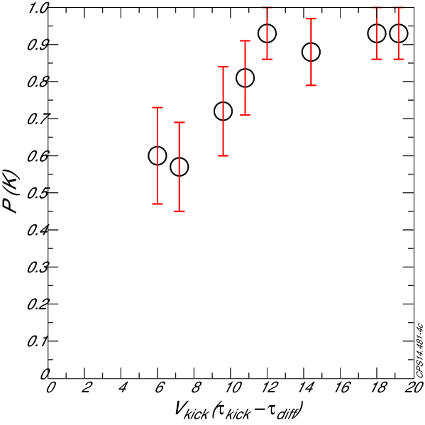
Figure 4: Consider the results from table 1 with a constant prior, for the 2T, 2MA, JET plasma 83440, that had 10.2MW of neutral beam heating and 7.5$\times$10²²s^-1 Deuterium gas fuelling. The probability of a kick triggering an ELM is plotted (vertical axis), versus the product of kick duration ($\tau_{kick}$) minus the 1.3ms JET vacuum-vessel diffusion time ($\tau_{diff}$), and the kick voltage ($V_{kick}$). The error bars are the standard deviations of $P(K)$ that are given in table 1. When $V_{kick}(\tau_{kick}-\tau_{diff})$ exceeds 12Wb (Volt seconds), the probability of a kick triggering an ELM appears to reach a maximum that is close to 1. (Higher values of $P(K)$ are only possible with a larger number of kicks to improve the statistics, for which case the error bars will also be reduced.)

We know that for JET there is a delay $\tau_{diff}$ of order 1.3ms for the magnetic field to diffuse through the vacuum vessel, but otherwise we might expect the maximum in the perturbation due to a kick to be proportional to the voltage multiplied by the length of the kick. If we subtract off the $\tau_{diff}=$1.3ms delay from the kick’s duration (there will continue to be a small increase in the plasma perturbation for a short period after the kick stops or reverses, but we will neglect this), then multiply it by the voltage of the kick, this should be approximately proportional to the maximum magnetic perturbation due to a kick. Plotting this against the probability of the kick being successful (figure 4), it appears that the threshold for kick success in this particular JET plasma, is a perturbation (to the plasma) of order 12 Wb. In other words,for this plasma it appears that if the product of kick duration minus the 1.3ms diffusion time, and voltage (i.e. $V_{kick}(\tau_{kick}-\tau_{diff})$), exceeds 12 Wb, then the kicks were almost 100% successful. Clearly this estimate needs refining with improved statistics (i.e. more experimental data), and a more accurate modelling of the peak magnetic perturbation to the plasma (by modelling how the magnetic field perturbation diffuses through the vessel), but both of these are possible. This analysis can be repeated for different pulse types to obtain the requirements for triggering ELMs; or alternately to determine the maximum perturbations a control system can apply while still ensuring a low risk of triggering an ELM.

VI.3 What triggers an ELM?

Once the thresholds for which ELMs are triggered are known, then modelling can determine the values of physical quantities such as the diffusing magnetic fields and currents, when those thresholds are approached and passed. By determining which processes are present, absent, increasing, or decreasing, hopefully we will be able to establish the mechanisms by which ELMs are being induced. For example, the rate of increase of the kick will determine how edge-localised any kick-induced currents will be. A short but rapidly increasing kick would be expected to produce strong but very localised current perturbations to the plasma’s edge, but a longer and weaker kick would allow a weaker current perturbation to diffuse further into the plasma. Peeling and peeling-ballooning modes WebsterGimblettPRL ; Laval ; Lortz ; Hegna ; Connor are widely recognised candidates for driving edge instabilities WebsterRev ; Groebner , and are driven increasingly unstable by increasingly strong currents at the plasma’s edge. Therefore they might be expected to be more strongly destabilised by a strong radially edge-localised current perturbation, as would be greatest with the most rapidly increasing kicks, and smallest with a longer and weaker kick. However for the example analysed here, the product of kick size and duration was found to be more important than the rate at which the kick was produced. Thorough modelling of these processes is probably required to understand with certainty whether the peeling mode is involved in the kick-triggering of ELMs, but the initial evidence just discussed suggests that another mechanism might be important. A detailed modelling and discussion of the processes that occur during a kick is beyond the scope of this paper, but there is enough evidence presented here to indicate that a systematic experimental investigation using the analysis tools in this paper can help clarify how a kick triggers an ELM; and possibly how ELMs are triggered more generally.

VII Conclusions

We have considered the generic problem of assessing whether an otherwise quasi-random event such as an edge-localised plasma instability (an “ELM”), has been triggered by an external influence. The specific problem of assessing the success of experiments to deliberately trigger ELMs by rapid vertical displacements of the plasma has been analysed in detail, leading to a simple set of rigorously derived formula to estimate the kick-triggering probability and its accuracy. The advantage of the method is its rigour. For example, we can now assert with confidence that vertical kicks with a voltage of only 3kV were in some cases triggering ELMs. This was unexpected, and has never previously been demonstrated. The method allows the success of kicks to be quantitatively assessed with unprecedented accuracy, allowing systematic studies to quantitatively determine how kick-triggering success depends on properties such as their duration, amplitude, and the peak magnetic field perturbation it produces. In the example considered (figure 4), the probability of a kick being successful increased approximately linearly with $V_{kick}(\tau_{kick}-\tau_{diff})$ until reaching a maximum of approximately 1 at approximately 12Wb ($V_{kick}$ is the vertical control system voltage, $\tau_{kick}$ is the duration of this step in voltage, $\tau_{diff}$ is JET’s vacuum vessel diffusion time). More generally, it is likely that analogous calculations and direct adaptations of the method presented here can be used to help distinguish cause from accidental correlation of quasi-random events in other circumstances.

Appendix

Appendix A The sum and product rules

The basic sum and product rules of Bayesian probability theory Jaynes can be used to derive the key formulas used in this paper. Firstly consider Eq. (3), noting that,

$$\begin{array}[]{ll}P(A,B|C)+P(A,\bar{B}|C)&=\left[P(B|A,C)+P(\bar{B}|A,C)\right]P(A|C)\\ &=P(A|C)\end{array}$$ (34)

where the 1st line uses the basic product rule Eq. (1), and the 1st-2nd line uses the basic sum rule Eq. (2). Next using the product rule to expand $P(A,B|C)=P(A|B,C)P(B|C)$ and $P(A,\bar{B}|C)=P(A|\bar{B},C)P(\bar{B}|C)$, then (34) expands to gives,

$$P(A|C)=P(A|B,C)P(B|C)+P(A|\bar{B},C)P(\bar{B}|C)$$ (35)

which is Eq. (3). If we replace $A$ with $t$, $B$ with $K$, and $C$ with $\tau_{m}$, then we have,

$$P(t|\tau_{m})=P(t|K,\tau_{m})P(K|\tau_{m})+P(t|\bar{K},\tau_{m})P(\bar{K}|\tau_{m})$$ (36)

which is Eq. 4, and gives $P(t|\tau_{m})$ the probability density of observing an ELM at time $t$ after a kick at time $\tau_{m}$, in terms of $P(t|K,\tau_{m})$ the probability density of observing an ELM at time $t$ after a kick at time $\tau_{m}$ successfully triggers an ELM, and $P(t|\bar{K},\tau_{m})$ the probability density of observing an ELM at time $t$ after a kick at time $\tau_{m}$ fails to trigger an ELM. The quantity $P(K|\tau_{m})$ is the probability of a kick being successful, given that the kick was at time $\tau_{m}$. As noted in the main text, the sum rule requires that $P(\bar{K}|\tau_{m})=1-P(K,\tau_{m})$.

Appendix B Correlations between ELMs and kicks

To assess how much correlations between the ELMs’ natural frequency and the kick frequency have the potential to influence the estimate, we consider a situation where an ELM has naturally occurred within the time window $\tau_{m}$ to $\tau_{m}+\Delta\tau$ that is usually associated with kick-triggered ELMs, and where the average ELM waiting time $\bar{t}$ equals the time between kicks $\tau_{m}-\tau_{m-1}$. Assuming the distribution of ELM waiting times is reasonably approximated by a Gaussian distribution with $P(t)=(1/\sqrt{2\pi\sigma^{2}})\exp\{-(t-\bar{t})^{2}/2\sigma^{2}\}$, that can often be the case for type I ELMs WebsterDendy2013 , then the probability $p$ of an ELM between $\bar{t}$ to $\bar{t}+\Delta\tau$ is,

$$p\simeq\Delta\tau P(\bar{t})=\frac{1}{\sqrt{2\pi}}\frac{\Delta\tau}{\sigma}$$ (37)

The probability of a sequence of $m$ ELMs within: $\bar{t}$ to $(\bar{t}+\Delta\tau)$, $2\bar{t}$ to $(2\bar{t}+\Delta\tau)$, … , $m\bar{t}$ to $(m\bar{t}+\Delta\tau)$, is then simply $p^{m}$, giving the number of correlated ELMs that we would expect to observe as,

$$\langle m\rangle=\frac{\sum_{m=1}^{\infty}mp^{m}}{\sum_{m=1}^{\infty}p^{m}}=\frac{p\frac{\partial}{\partial p}\sum_{m=1}^{\infty}p^{m}}{\sum_{m=1}^{\infty}p^{m}}=\frac{1}{1-p}$$ (38)

where we used $\sum_{m=1}^{\infty}p^{m}=p/(1-p)$ to evaluate the sums. $\langle m\rangle$ tends to $1$ as $\Delta\tau/\sigma\rightarrow 0$, or infinity as $\Delta\tau/\sigma\rightarrow 1$. Most of the cases we are interested in have $\Delta\tau/\sigma\ll 1$. For those cases, even if $\bar{t}=\tau_{m}-\tau_{m-1}$, then the number of ELMs to be incorrectly counted as “triggered” by the kicks will be small, with $\langle m\rangle<2$ for $\Delta\tau/\sigma<0.5$, and of order $1$ for $\Delta\tau/\sigma\ll 1$. In most cases, $\bar{t}$ will be substantially different to $\tau_{m}-\tau_{m-1}$, and the potential influence of correlations can be neglected entirely.

References

- (1) J. Wesson Tokamaks (Oxford University Press, Oxford, 1997).
- (2) H. Zohm, Plasma Physics and Controlled Fusion 38, 105, (1996).
- (3) A.W. Degeling, Y.R. Martin, J.B. Lister, L. Villard, A.N. Dokouka, V.E. Lukash, R.R. Khayrutdinov, Plasma Phys. Control. Fusion, 45, 1637, (2003).
- (4) P.T. Lang, A.W. Degeling, J.B. Lister, Y.R. Martin, P.J. Mc Carthy, A.C.C. Sips, W. Suttrop, G.D. Conway, L. Fattorini, O. Gruber, L.D. Horton, A. Herrmann, M.E. Manso, M. Maraschek, V. Mertens, A. M ck, W. Schneider, C. Sihler, W. Treutterer, H. Zohm and ASDEX Upgrade Team, Plasma Phys. Control. Fusion, 46, L31, (2004).
- (5) Y. Liang, Fusion Science and Technology 59, 586, (2011).
- (6) P.T. Lang, A. Loarte, G. Saibene, L.R. Baylor, M. Becoulet, M. Cavinato, S. Clement-Lorenzo, E. Daly, T.E. Evans, M.E. Fenstermacher, Y. Gribov, L.D. Horton, C. Lowry, Y. Martin, O. Neubauer, N. Oyama, M.J. Schaffer, D. Stork, W. Suttrop, P. Thomas, M. Tran, H.R. Wilson, A. Kavin, O. Schmitz Nucl. Fusion 53, 043004, (2013).
- (7) F.G. Rimini, F. Crisanti, R. Albanese, G. Ambrosino,M. Ariola,G. Artaserse, T. Bellizio, V. Coccorese, G. De Tommasi, P. De Vries, P. J. Lomas, F. Maviglia, A. Neto, I. Nunes, A. Pironti, G. Ramogida, F. Sartori, S.R. Shaw, M. Tsalas, R. Vitelli, L. Zabeo, JET EFDA Contributors, Engineering and Design, 86, 539-543, (2011).
- (8) E.T. Jaynes “Probability Theory the Logic of Science”, Cambridge University Press, (2003).
- (9) A.J. Webster and R.O. Dendy, Phys. Rev. Lett. 110, 155004, (2013).
- (10) D.S. Sivia “Data Analysis a Bayesian Tutorial” Oxford University Press, Great Clarendon Street, Oxford, (1996).
- (11) L.S. Schulman “Techniques and Applications of Path Integration” John Wilely & Sons, Inc. (1981).
- (12) S. Brezinsek, T. Loarer, V. Phillips, H.G. Esser, S. Grünhagen, R. Smith, R. Felton, J. Banks, P. Belo, A. Boboc, J. Bucalossi, M. Clever, J.W. Coenen, I. Coffey, D. Douai, M. Freisinger, D. Frigione, M. Groth, A. Huber, J. Hobirk, S. Jachmich, S. Knipe, K. Krieger, U. Kruezi, G.F. Matthews, A.G. Meigs, F. Nave, I. Nunes, R. Neu, J. Roth, M.F. Stamp, S. Vartagnian, U. Samm, and JET EFDA contributors, Nuclear Fusion, 53, 083023, (2013).
- (13) A.J. Webster, Nucl. Fusion, 52, 114023, (2012).
- (14) R.J. Groebner, C.S. Chang, J.W. Hughes, R. Maingi, P.B. Snyder, X.Q. Xu, J.A. Boedo, D.P. Boyle, J.D. Callen, J.M. Canik, I. Cziegler, E.M. Davis, A. Diallo, P.H. Diamond, J.D. Elder, D.P. Eldon, D.R. Ernst, D.P. Fulton, M. Landreman, A.W. Leonard, J.D. Lore, T.H. Osborne, A.Y. Pankin, S.E. Parker, T.L. Rhodes, S.P. Smith, A.C. Sontag, W.M. Stacey, J. Walk, W. Wan, E.H.-J. Wang, J.G. Watkins, A.E. White, D.G. Whyte, Z. Yan, E.A. Belli, B.D. Bray, J. Candy, R.M. Churchill, T.M. Deterly, E.J. Doyle1, M.E. Fenstermacher, N.M. Ferraro, A.E. Hubbard, I. Joseph, J.E. Kinsey, B. LaBombard, C.J. Lasnier, Z. Lin, B.L. Lipschultz, C. Liu, Y. Ma, G.R. McKee, D.M. Ponce, J.C. Rost, L. Schmitz, G.M. Staebler, L.E. Sugiyama, J.L. Terry, M.V. Umansky, R.E. Waltz, S.M. Wolfe, L. Zeng and S.J. Zweben, Nucl. Fusion, 53, 093024, (2013).
- (15) A.J. Webster, S.J. Webster, and JET-EFDA Contributors, arXiv:1311.1942, Accepted for publication in Physics of Plasmas, (2014).
- (16) G. Laval, R. Pellat, J.S. Soule, Phys. Fluids, 17, 835, (1974).
- (17) D. Lortz, Nucl. Fusion 15, 49, (1975).
- (18) A.J. Webster, C.G. Gimblett, Phys. Rev. Lett. 102, 035003, (2009).
- (19) C.C. Hegna, J.W. Connor, R.J. Hastie, H.R. Wilson, Phys. Plasmas, 3, 584, (1996).
- (20) J.W. Connor, R.J. Hastie, H.R. Wilson, R.L. Miller, Phys. Plasmas, 5, 2687, (1998).
- (21) G.T.A. Huysmanns, Plasma Phys. Controlled Fusion, 47, 2107, (2005).