Higgs Model Coupled to Dark Photons

Abstract

A dark sector containing a Higgs field and a dark photon coupled to visible photons via a small kinetic mixing is considered. The mass of the dark gauge boson becomes rescaled by the parameter involved in the kinetic mixing. We also calculate the total annihilation cross section for scalar Higgs interacting with an external field and show that exhibits Sommerfeld enhancement. The model can be extended to a $SU(3)\times SU(2)\times U(1)$ dark sector. The mass of the dark $Z$ boson increases due to the kinetic mixing.

Introduction

Since the seventies it has been observed that the gamma ray spectrum coming from the galactic center possesses a 511 keV emission line consistent with a copious annihilation of electron-positron pairs jo ; le ; sha ; ki ; atti ; ve ; kn ; wei ; tee . Nonetheless, the calculated rate of $\sim 10^{42}$ annihilations per second exceeds in several order of magnitude the creation rate of electron-positron pairs from the interaction of cosmic rays with the interstellar medium. This and other anomalies in the cosmic ray observations (see arkani for a summary) could be naturally explained by assuming that the overabundance of matter-antimatter pairs is due to an (Sommerfeld) enhancement of the total cross section of dark matter annihilation. This opens a possibility for new physics in order to address the question of how ordinary and dark matter interact to produce this enhancement.

Several routes have been proposed to explain this puzzle (see e.g. arkani , pospe or review0 for recent references), although the most popular approaches to dark matter are WIMPS’s and new interactions beyond the standard model beyond .

In this paper we propose a simple model containing a hidden sector composed of a dark Higgs field and a dark photon coupled with visible photons through a small kinetic mixing holdom . In the first section, we show that this interaction is enough to produce an enhancement of electromagnetic processes in the dark sector. In the second part, we analyze the consequences of kinetic mixing in an extended dark model $SU(3)\times SU(2)\times U_{Y}(1)\times U_{Y^{\prime}}(1)$, where $U_{Y^{\prime}}(1)$ is the visible hypercharge. The mass of the dark vector boson $Z$ turns out to be bigger than the usual $Z$.

I A Toy Model

This first part is devoted to the problem of determining the total annihilation cross section for a Higgs model coupled to dark photons, explicitly showing the enhancement. For concreteness, let us start considering the following model

$${\cal L}={\cal L}_{Dark}+{\cal L}_{I},$$ (1)

where ${\cal L}_{Dark}$ is a scalar electrodynamics-like Lagrangian for the hidden sector

$${\cal L}_{Dark}=|D(A)\phi|^{2}-m^{2}|\phi|^{2}-\frac{\lambda}{2}(|\phi|^{2})^{2}-\frac{1}{4e^{2}_{A}}F_{\mu\nu}(A)F^{\mu\nu}(A),$$ (2)

where $A_{\mu}$ and $\phi$ are dark fields and $D_{\mu}(A)=\partial_{\mu}-iA_{\mu}$. Now suppose that at some energy scale an interaction with the visible photon appears. The Lagrangian ${\cal L}_{I}$ is then given by

$${\cal L}_{I}=-\frac{1}{4e^{2}_{B}}F_{\mu\nu}(B)F^{\mu\nu}(B)+\frac{\gamma}{2}F_{\mu\nu}(A)F^{\mu\nu}(B),$$ (3)

where $B_{\mu}$ is the visible photon, $F_{\mu\nu}(A)F^{\mu\nu}(B)$ is the kinetic mixing and $\gamma$ is a small dimensionless coefficient ring .

The quantum theory is described by the integral

$${\cal Z}=\int{\cal D}\phi{\cal D}\phi^{*}\int\left[{\cal D}A_{\mu}{\cal D}B_{\mu}\right]\,e^{iS[\phi,\phi^{*},A,B]}$$ (4)

where $\left[{\cal D}A_{\mu}{\cal D}B_{\mu}\right]$ is a compact notation that includes the gauge fixing and the Faddev-Popov determinant.

In order to obtain a mixture of visible and dark coupling constant, it is convenient to perform the change of variables

$$A^{\prime}_{\mu} = A_{\mu},$$

$$B^{\prime}_{\mu} = B_{\mu}-\gamma e^{2}_{B}A_{\mu},$$

which diagonalizes ${\cal L}_{I}-\frac{1}{4e^{2}_{A}}F_{\mu\nu}(A)F^{\mu\nu}(A)$ as follows

$$-\frac{1}{4{\tilde{e}}^{2}}F^{2}(A^{\prime})-\frac{1}{4e^{2}_{B}}F^{2}(B^{\prime}),$$ (5)

but paying the price of redefining the electric charge $e_{A}$ by the effective charge ${\tilde{e}}$, i.e.

$${\tilde{e}}=\frac{e_{A}}{\sqrt{1-(\gamma e_{B}e_{A})^{2}}}.$$ (6)

In other words, (1) must be written as

$${\cal L}=|D(A)\phi|^{2}-m^{2}|\phi|^{2}-\frac{\lambda}{2}(|\phi|^{2})^{2}-\frac{1}{4{\tilde{e}}^{2}}F^{2}(A)-\frac{1}{4e^{2}_{B}}F^{2}(B).$$ (7)

The path integral becomes

$${\cal Z} = \int{\cal D}\phi{\cal D}\phi^{*}\int\left[{\cal D}A_{\mu}{\cal D}B_{\mu}\right]\,e^{i\int d^{4}x\left(|D(A)\phi|^{2}-m^{2}|\phi|^{2}-\frac{\lambda}{2}(|\phi|^{2})^{2}-\frac{1}{4{\tilde{e}}^{2}}F^{2}(A)-\frac{1}{4e^{2}_{B}}F^{2}(B)\right)}$$ (8)

$$= {\cal N}\int{\cal D}\phi{\cal D}\phi^{*}\int{\cal D}A_{\mu}\,e^{i\int d^{4}x\left(|D(A)\phi|^{2}-m^{2}|\phi|^{2}-\frac{\lambda}{2}(|\phi|^{2})^{2}-\frac{1}{4{\tilde{e}}^{2}}F^{2}(A)\right)}$$

$$= {\cal N}\int{\cal D}\phi{\cal D}\phi^{*}\int{\cal D}A_{\mu}\,e^{i\int d^{4}x{\cal L}},$$

where the $B_{\mu}$ field have been absorbed in the normalization constant ${\cal N}$, leaving the effective action as

$${\cal L}_{eff}=|D(A)\phi|^{2}-m^{2}|\phi|^{2}-\frac{\lambda}{2}(|\phi|^{2})^{2}-\frac{1}{4{\tilde{e}}^{2}}F^{2}(A),$$ (9)

which is a Higgs model with a nontrivial rescaling of the electric charge. Furthermore, we can hide the charge $\tilde{e}$ by redefining the potential $A_{\mu}$ as

$$A_{\mu}\to{{\tilde{e}}}{A}_{\mu},$$ (10)

so that the effective Lagrangian (9) becomes

$${\cal L}_{eff}=|D(A)\phi|^{2}-m^{2}|\phi|^{2}-\frac{\lambda}{2}(|\phi|^{2})^{2}-\frac{1}{4}F^{2}(A),$$ (11)

where the redefined covariant derivative is

$$D_{\mu}[A]=\partial_{\mu}-i{\tilde{e}}A_{\mu}.$$

Therefore, a first conclusion is that the kinetic mixing with the visible photon is equivalent to shield the electric charge $e_{A}$. The effective model is just an abelian Higgs model with the coupling constant ${\tilde{e}}$ instead of $e$. This conclusion is valid not only for the Higgs field. Any other particle in the dark sector coupled to the dark photon would have its charge redefined in the same way.

Now we can perform spontaneous symmetry breaking. Using the Kibble parametrization, the scalar field can be written as

$$\phi=\frac{1}{\sqrt{2}}\left(v+h\right)\,e^{\frac{i}{v}\xi},$$ (12)

where $v$ is the minimum of the potential, i.e.

$$v=\sqrt{-\frac{2m^{2}}{\lambda}},$$ (13)

and $h$ and $\xi$ are the Higgs and Goldstone bosons.

Inserting (12) in (11) we obtain

$${\cal L}_{eff} = \frac{1}{2}(\partial h)^{2}-\frac{m^{2}}{2}(v+h)^{2}-\frac{\lambda}{8}(v+h)^{4}+\frac{{\tilde{e}}^{2}}{2}(v+h)^{2}A_{\mu}A^{\mu}$$ (14)

$$-\frac{1}{4}F_{\mu\nu}(A)F^{\mu\nu}(A)+\frac{(v+h)^{2}}{v}\partial^{\mu}\xi\left[\frac{1}{2v}\partial_{\mu}\xi-\tilde{e}A_{\mu}\right].$$

Choosing the U-gauge, the last term in (14) vanishes, therefore

$${\cal L}_{eff} = \frac{1}{2}(\partial h)^{2}-\frac{m^{2}}{2}(v+h)^{2}-\frac{\lambda}{8}(v+h)^{4}+\frac{{\tilde{e}}^{2}}{2}(v+h)^{2}A_{\mu}A^{\mu}-\frac{1}{4}F_{\mu\nu}(A)F^{\mu\nu}(A),$$ (15)

$$= \frac{1}{2}(\partial h)^{2}-m^{2}h^{2}-\frac{1}{4}F_{\mu\nu}(A)F^{\mu\nu}(A)+\frac{m^{2}_{A}}{2}A_{\mu}A^{\mu}+\frac{{\tilde{e}}^{2}}{2}h^{2}A_{\mu}A^{\mu}+\cdots$$

from where we see that

$$m_{A}={\tilde{e}}v,$$ (16)

is the dark photon mass.

Already at this level we see that the effect of kinetic mixing not only amplifies the coupling constant but also the gauge boson mass. The same will happen when considering a more realistic model, where the dark $Z$ boson will have a rescaled mass.

Since the model under consideration has a redefined coupling constant, the cross section of any process involving this coupling must have an enhancement. To make this fact explicit, let us calculate the total cross section of a simple process. For example, consider FIG. 1,

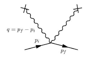
Figure 1: Higgs interacting with an external massive vector field.

which is described by the term

$$\frac{{\tilde{e}}^{2}}{2}h^{2}A_{\mu}A^{\mu},$$

where $A_{\mu}A^{\mu}$ is considered –as a simple application– an external field.

The $S$-matrix elements are

$$<f|S|i>=(-\frac{i}{2}{\tilde{e}}^{2}\eta_{\mu\nu})\frac{1}{\sqrt{2E_{f}2E_{i}}V}\int d^{4}xe^{i(p_{f}-p_{i})\cdot x}A^{\mu}(x)A^{\nu}(x),$$ (17)

with $V$ is a normalization volume and the product $A^{\mu}(x)A^{\nu}(x)$ is a convolution integral in the Fourier space, i.e.

$$<f|S|i>=(-\frac{i}{2}{\tilde{e}}^{2}\eta_{\mu\nu})\frac{1}{\sqrt{2E_{f}2E_{i}}V}\int d^{4}kA^{\mu}(q-k)A^{\nu}(k),$$ (18)

where $q=p_{f}-p_{i}$ is the transferred momentum.

As the external field is massive, it can be expressed as

$$A^{\mu}(x)=\frac{\alpha\,e^{-m_{A}r}}{r}\longrightarrow A^{\mu}(q)=\delta(q_{0})\frac{2\alpha}{{\bf q}^{2}+m^{2}_{A}}\eta^{\mu 0},$$ (19)

where $\alpha$ is the source charge generating the external field. For simplicity, $\alpha$ will be normalized to 1.

Using these results, $<f|S|i>$ is

$$<f|S|i>=-(i{\tilde{e}}^{2})\frac{\delta(q_{0})}{\sqrt{E_{f}E_{i}}V}\int d^{3}k\frac{1}{(|{\bf q}-{\bf k}|^{2}+m^{2}_{A})}\frac{1}{({\bf k}^{2}+m^{2}_{A})}.$$ (20)

In order to compute (20) we use a Feynman parameterization and we get

$$<f|S|i>=-(i{\tilde{e}}^{2})\frac{2\pi^{2}\delta(q_{0})}{\sqrt{E_{f}E_{i}}V}\frac{1}{|{\bf q}|}\arcsin\frac{|{\bf q}|}{\sqrt{{\bf q}^{2}+4m_{A}^{2}}}.$$ (21)

The differential cross section is given by

$$d\sigma=\frac{1}{|{\bf j_{in}}|}\frac{|S_{fi}|^{2}}{T}\frac{Vd^{3}p_{f}}{(2\pi)^{3}},$$ (22)

where ${\bf j_{in}}={\bf v_{i}}/V$ is the incoming current and $T$ is a time normalization parameter drell .

Collecting everything we get

$$\frac{d\sigma}{d\Omega_{f}}=\frac{{\tilde{e}}^{4}}{4}\left|i\frac{1}{2|{\bf p}|\sin\frac{\theta}{2}}\arcsin\frac{\sin\frac{\theta}{2}}{\sqrt{\sin^{2}\frac{\theta}{2}+\frac{m^{2}_{A}}{|{\bf p}|^{2}}}}\right|^{2}=|f(\theta,\phi)|^{2},$$ (23)

where the term between $|...|^{2}$ is just the scattering amplitude and $|{\bf p}|=|{\bf p}_{f}|=|{\bf p}_{i}|$.

The calculation of the total annihilation cross section is most easily done by using the optical theorem, namely

$$\sigma_{T}=\int|f(\theta,\phi)|^{2}d\Omega=\frac{4\pi}{|{\bf p}|}{\cal I}\mbox{m}\left[f(\theta=0)\right],$$ (24)

and with the help of the identity

$$\lim_{x\to 0}\frac{1}{x}\arcsin\frac{x}{\sqrt{x^{2}+a^{2}}}=\frac{1}{a},$$ (25)

the total cross section becomes

$$\sigma_{T}=\frac{\pi\tilde{e}^{4}}{4|{\bf p}|\,m_{A}},$$ (26)

which shows the Sommerfeld enhancement at low energies for this particular process.

As mentioned above, although this calculation was made for a particular interaction, FIG. 1, it is clear that any other electromagnetic process in the dark sector will have an enhanced cross section since it will depend on the rescaled electric charge. Accordingly, the conclusion that the coupling to the visible photon induces an enhancement in the interactions is also true for more complicated processes.

To higher orders –i.g., $n$-th order– the total cross section should be proportional to $(1-(\gamma e_{B}e_{A})^{2})^{-n/2}$ and therefore negligibly small in comparison to the tree level processes.

II Extension to $SU(3)\times SU(2)\times U(1)$

In order to extend these results to the case $SU(3)\times SU(2)\times U_{Y}(1)$, one proceed as follows; first, we consider the dark non abelian fields $G_{\mu}=G^{a}_{\mu}\lambda^{a}$ and $A_{\mu}=A^{a}_{\mu}\tau^{\alpha}$, where $\lambda^{a}$ and $\tau^{\alpha}$ are the generators of $SU(3)$ and $SU(2)$ respectively, while the dark abelian field will be denoted by $B_{\mu}$.

Following the above ideas, the non abelian fields will remain untouched, but the abelian field dynamics will be modified by extending the gauge group to $SU(3)\times SU(2)\times U_{Y}(1)\times U_{Y^{\prime}}(1)$, where $U_{Y^{\prime}}(1)$ is associated to the visible photon $B^{\prime}_{\mu}$. Accordingly, consider the Lagrangian

$${\cal L}={\cal L}_{\text{matter}}+{\cal L}_{\text{gauge}},$$ (27)

where ${\cal L}_{\text{matter}}$ denotes all matter fields in the dark sector, including a dark Higgs field and their interactions with the gauge fields.

We are now interested in the gauge sector. Similarly to the above model, we include the visible field $B^{\prime}_{\mu}$, coupled to $B_{\mu}$ through a kinetic mixing. The Lagrangian gets diagonalized

$${\cal L}_{\text{gauge}} = -\frac{1}{4}\text{tr}F^{2}(G)-\frac{1}{4}\text{tr}F^{2}(A)-\frac{1}{4{{g^{\prime}}^{2}}}F^{2}(B)-\frac{1}{4{{g^{\prime\prime}}^{2}}}F^{2}(B^{\prime})+\frac{\gamma}{2}F(B)F(B^{\prime})$$ (28)

$$= -\frac{1}{4}\text{tr}F^{2}(G)-\frac{1}{4}\text{tr}F^{2}(A)-\frac{1}{4{\tilde{g}}}F^{2}(B)-\frac{1}{4g^{\prime\prime 2}}F^{2}({\tilde{B}}),$$

where the coupling constant $g^{\prime}$ gets redefined

$${\tilde{g}}=\frac{g^{\prime}}{\sqrt{1-(g^{\prime}{g^{\prime\prime}}\gamma)^{2}}}\equiv\frac{g^{\prime}}{\sqrt{1-\chi^{2}}},$$ (29)

and the $\tilde{B}_{\mu}$ field is defined as

$${\tilde{B}}_{\mu}=B^{\prime}_{\mu}-\gamma g^{\prime\prime 2}B_{\mu}.$$

From the path integral formulation, the field ${\tilde{B}}$ is decoupled from the dynamics of the other fields and the only relic of the kinetic mixing emerges from the rescaled coupling (29). By redefining $B_{\mu}$ in (28) as

$$\frac{B_{\mu}}{{\tilde{g}}}\to{\cal B}_{\mu}.$$

the covariant derivative turns out to be

$$D_{\mu}=\partial_{\mu}-ig_{S}G_{\mu}-igA_{\mu}-i{\tilde{g}}{\cal B}_{\mu}$$ (30)

and therefore the dark sector becomes $SU(3)\times SU(2)\times U(1)$ with an effective hypercharge.

We can now follow the lines of the Higgs mechanism in the usual way. The mass of the dark Z boson gets rescaled as

$$M_{Z}\to\frac{M_{Z}}{\sqrt{1-\chi^{2}}}\equiv M_{Z^{\prime}},$$ (31)

as opposite to the masses of the $W$ which remains unchanged. Note that $M_{Z^{\prime}}>M_{Z}$.

As a final remark, due to the redefinition of the $Z$ mass, the Fermi coupling constant $G_{F}$ also gets rescaled. Since $g$, the coupling constant of the weak sector, does not change, $G_{F}$ gets redefined

$$G_{F}=\frac{g^{2}}{M^{2}_{Z}}\rightarrow G^{\prime}_{F}=\frac{g^{2}}{M^{2}_{Z^{\prime}}},$$

which implies

$$\frac{G^{\prime}_{F}}{G_{F}}=1-\chi^{2}<1.$$ (32)

This agrees with some phenomenological considerations santa .

References

• (1) W. N. Johnson, III, F. R. Harnden, Jr., and R. C. Haymes, Ap. J. 172, L1 (1972).
• (2) M. Leventhal, Ap. J 183, L147 (1973).
• (3) G. H. Share, R. L. Kinzer, J. D. Kurfess, D. C. Messina, W. R. Purcell, E. L. Chupp, D. J. Forrest, and C. Reppin, ApJ 326, 717 (1988).
• (4) R. L. Kinzer et al., Astrophys. J.559, 282 (2001).
• (5) D. Attie, B. Cordier, M. Gros, P. Laurent, S. Schanne, G. Tauzin, P. von Ballmoos, L. Bouchet, P. Jean, J. Knödlseder, et al., A$\&$A 411, L71 (2003), astro-ph/0308504.
• (6) G. Vedrenne, J.-P. Roques, V. Schönfelder, P. Mandrou, G. G. Lichti, A. von Kienlin, B. Cordier, S. Schanne, J. Knödlseder, G. Skinner, et al., A $\&$ A 411, L63 (2003).
• (7) J. Knödlseder et al., Astron. Astrophys.411, L457 (2003), astro-ph/0309442.
• (8) G. Weidenspointner et al., A$\&$A 450, 1013 (2006), astro-ph/0601673.
• (9) B. J. Teegarden, K. Watanabe, P. Jean, J. Knodlseder, V. Lonjou, J. P. Roques, G. K. Skinner, P. von Ballmoos, G. Weidenspointner, A. Bazzano, et al., Ap. J621, 296 (2005), astro-ph/0410354.
• (10) N. Arkani-Hamed, D. P. Finkbeiner, T. R. Slatyer and N. Weiner, Phys. Rev. D 79, 015014 (2009) [arXiv:0810.0713 [hep-ph]].
• (11) M. Pospelov and A. Ritz, Phys. Lett. B 671, 391 (2009) [arXiv:0810.1502 [hep-ph]].
• (12) A. Fradette, M. Pospelov, J. Pradler and A. Ritz, arXiv:1407.0993 [hep-ph].
• (13) For a review see e.g., P. Langacker, “The standard model and beyond,” Boca Raton, USA: CRC Pr. (2010) 663 pp.
• (14) B. Holdom, Phys. Lett. B 166, 196 (1986).
• (15) M. Ahlers, H. Gies, J. Jaeckel, J. Redondo and A. Ringwald, Phys. Rev. D 77, 095001 (2008) [arXiv:0711.4991 [hep-ph]]; S. A. Abel, J. Jaeckel, V. V. Khoze and A. Ringwald, Phys. Lett. B 666, 66 (2008) [hep-ph/0608248].
• (16) J. D. Bjorken and S. D. Drell, “Relativistic quantum mechanics,”, Mc Graw Hill, (1965).
• (17) M. S. Bilenky and A. Santamaria, hep-ph/9908272; E. W. Kolb and M. S. Turner, Phys.  Rev.  D 36 (1987) 2895; A. Manohar, Phys.  Lett. B 192 (1987) 217; D. A. Dicus, S. Nussinov, P. B. Pal and V. L. Teplitz, Phys.  Lett. B 218 (1989) 84; M. S. Bilenky, S. M. Bilenky and A. Santamaria, Phys. Lett. B 301 (1993) 287; M. S. Bilenky and A. Santamaria, Phys.  Lett. B 336 (1994) 91 [hep-ph/9405427]; E. Massó and R. Toldrá, Phys.  Lett. B 333 (1994) 132 [hep-ph/9404339].