Density Classification Quality of the Traffic-majority Rules

Abstract

The density classification task is a famous problem in the theory of cellular automata. It is unsolvable for deterministic automata, but recently solutions for stochastic cellular automata have been found. One of them is a set of stochastic transition rules depending on a parameter $\eta$, the traffic-majority rules.

Here I derive a simplified model for these cellular automata. It is valid for a subset of the initial configurations and uses random walks and generating functions. I compare its prediction with computer simulations and show that it expresses recognition quality and time correctly for a large range of $\eta$ values.

1 Introduction

This is an analysis of a specific solution by Fatès [3] of the so-called density classification task for cellular automata.

This task is an example of a synchronisation problem. In it, several independent agents (the cells) must reach a common state, that one which was initially that of the majority of them. The cells have finite memory and restricted knowledge of each other’s states, so that none of them knows the whole system. Fatès published a solution that relies on a randomised algorithm; while he proved that the algorithm is successful with high probability, he provided only rough bounds for the probability of success and the time it takes.

This article analyses the algorithm in detail for a subset of initial conditions and provides improved bounds. It is an exploration of the use of random walks and generating functions for the understanding of cellular automata. The analysis turns out to be quite complex. I will therefore only consider a subset of all possible initial configurations and will use simplifications in the stochastic model. We will however see that the simplifications have no great influence: the model is valid in more cases than one would expect according to its derivation.

I now will describe cellular automata and the density classification task in detail and then proceed to the analysis of the solution.

1.1 Cellular Automata

Cellular Automata are discrete dynamical systems that are characterised by local interactions. The following semi-formal definition is intended to clarify the nomenclature used here.

A cellular automaton consists of a grid on which cells are located. The grid is usually $\mathbb{Z}$ or $\mathbb{Z}^{2}$, sometimes higher dimensional. It may also be cyclic, like $\mathbb{Z}/n\mathbb{Z}$. Every cell has a state, which belongs to a finite set that is the same for all cells. The system of all cells at a time is a configuration.

Time runs in discrete steps. At every time step a transition rule is applied to every cell, and it determines the state of that cell one time step later. All cells follow the same transition rule, and the state of each cell depends only on the state of the cell itself and that of a finite number of its neighbours at the previous time step. The locations of these neighbours relatively to the cell is also equal for all cells.

The transition rule can be deterministic or stochastic. In the latter case the rule determines for each cell and each possible state the probability that at the next time step the cell is in this state. For different cells these probabilities are stochastically independent.

A special class of deterministic automata are the Elementary Cellular Automata (ECA), popularised by Stephen Wolfram. They are the cellular automata with radius 1 and two states and usually designated by a number in Wolfram’s numbering scheme [17].

1.2 The Density Classification Task

Density Classification is a famous problem in the theory of cellular automata. In it, a one-dimensional cellular automaton, with $\mathbb{Z}/n\mathbb{Z}$ as grid and with two cell states, must evolve to a configuration with all cells in state 1 if the fraction of cells that are initially in state 1 is higher than a given critical density $\rho$, otherwise to the state where all cells are in state 0. In most cases the critical density is $\frac{1}{2}$.

Some ring sizes allow configurations in which the fraction of cells in state 1 is exactly $\rho$; they are usually excluded from consideration. In case of $\rho=\frac{1}{2}$ this means that $n$ must be odd.

The density classification task is important because it is a difficult problem for cellular automata. In a cellular automaton, no cell knows the system as a whole, and still they must cooperate according to information that none of them has. Another difficulty is that no cell in $\mathbb{Z}/n\mathbb{Z}$ is distinguished and could play the role of an organiser.

In fact, the density classification task is unsolvable for deterministic cellular automata, but that was found out only years after the problem was posed.

There are however solution for stochastic cellular automata. One of them is a parametric family of transition rules introduced by Fatès [3] that is analysed here.

1.3 What is a Solution?

Before we proceed, we need to clarify what exactly a solution of the density classification problem is. Apparently this has never been done for the general case.

The most natural definition would be that a transition rule solves the density classification problem if it classifies density correctly for every ring size. I will call this a strong solution; it is also the interpretation used by Land and Belew [10].

This definition is natural because it enforces a true computation of the cellular automaton: It excludes the trivial case of a transition rule of radius $\lceil\frac{n}{2}\rceil$ on a ring of $n$ cells that solves the classification problem in one step because each cell can see the whole ring.

In other cases, the algorithm depends on a parameter that must be adjusted according to the ring size. An example is the family of transition rules found by Briceño et al. [1]. They show that for every $\epsilon$ there is a transition rule which classifies an initial configuration correctly if its density is less that $\frac{1}{2}-\epsilon$ or greater than $\frac{1}{2}+\epsilon$. If the ring has less than $\epsilon^{-1}$ cells, all initial configurations have this property and are therefore classified correctly. Some configurations on larger rings are however classified incorrectly; so this rule is not a strong solution.

Nevertheless, it is no trivial algorithm, since no cell in such a solution sees the whole ring. I will therefore call a family of transition rules a weak solution if it contains for each ring size a rule that classifies density correctly and has a radius that is significantly smaller than the ring size.

1.4 Notes on the History of the Problem

It is not completely clear who first proposed the Density Classification Task. Apparently it became popular after Packard [15] used it as a test case for the “edge of chaos” hypothesis [11]. He used evolutionary programming to find cellular automata that are good classifiers; the fitness of a transition rule was related to the fraction of initial configurations it classifies correctly.

At that time, the best known approximate solution of the problem was a transition rule by Gács, Kurdiumov and Levin [7]. It had originally been proposed as a solution for a different problem, but it also solves the classification task correctly for 97% of the densities, in a cellular automaton with ring size 149. In later literature [5, 12, 13, 14] it was used as a benchmark for other approximate solutions and as an example for the concrete behaviour of an approximate solution of the problem.

Among the people who evolved cellular automata for density classification were Land and Belew. They found an automaton roughly as successful as the solution of Gács et al., but converging much faster. However, their “difficulties in evolving even better solutions led [them] to wonder whether such a CA actually exists” [10, Introduction], and they found the impossibility proof.

After that, researchers began to modify the task, trying to find variants that were solvable. Capcarrère, Sipper and Tomassini [2] modified the output specification: Their automaton is required to evolve to a configuration with the cells alternately in states 0 and 1, except for longer blocks of 0s (if the initial density was less than $\frac{1}{2}$) or longer blocks of 1s (if the density was lower than $\frac{1}{2}$). Their solution, which classifies all densities correctly, is the ECA rule with code number 184, the “traffic rule”.

One can also change the number of states in the cellular automaton. The initial and final configuration still have only cells in state 0 or 1, but in between more states are allowed. That is what Briceño et al. [1] did; their result is only a weak solution, as we have seen.

Fukś [5] changed instead the algorithm and applied two different cellular automata rules in succession. Initially, ECA 184 is applied for $\left\lfloor\frac{n-2}{2}\right\rfloor$ steps to generate the pattern of alternating 0 and 1 cells and either longer blocks of 0s or 1s. Then ECA 232 is run; it is the “majority rule” in which the next state of a cell is the state of the majority of the cells in its 3-cell neighbourhood. With it, the cell states that are in the minority slowly die out, and a configuration consisting completely of 0s or 1s is reached. It is a weak solution because the algorithm depends on the ring size.

Sipper, Capcarrère and Ronald [16] changed topology and output condition: Instead of using a ring they organised the cells as a finite line, with a cell at the left end that stays always in state 0 and a cell at the right end that stays always in state 1. Then their automaton evolves to a configuration where all cells in state 0 are at the left and those in state 1 are at the right—and their number unchanged—so the state of the cell in the middle is that of the majority. They compared the unsolvable original version of the problem [7] with the “easy” solutions—that by Capcarrère et al. [2] and their own—and concluded that

“density is not an intrinsically hard problem to compute. This raises the general issue of identifying intrinsically hard problems for such local systems, and distinguishing them from those that can be transformed into easy problems.” [16, p. 902]

Fukś [6] extended the task to stochastic cellular automata. His algorithm is a randomised version of the majority rule:

“empty sites become occupied with a probability proportional to the number of occupied sites in the neighborhood, while occupied sites become empty with a probability proportional to the number of empty sites in the neighborhood.” [6, Introduction]

The algorithm classifies density in the sense that the probability that the automaton reaches the configuration with all cells in state 1 grows with the fraction of 1s in the initial state. Thus it is more probable for a configuration with density $>\frac{1}{2}$ to evolve to a configuration of 1s than to one of 0s, and vice versa. The additional probability for a correct classification is however not very high [4, p. 233].

Fatès [4] then introduced the so-called “traffic-majority” rules—a family of transition rules that look like stochastic versions of the algorithm by Fukś [5]. Instead of applying his two rules in sequence, at every time step and for every cell either Rule 184 or Rule 232 is applied. The algorithm can be “tuned” to arbitrarily high classification qualities, but at a price: The higher the probability is for Rule 184, the better the classification—but it also becomes slower. Although there is as yet no formal proof, this is a sign that the algorithm is only a weak solution.

The traffic-majority rules will now be investigated in more detail.

2 Definitions

2.1 Notations and conventions

This section explains the notations I will use here. Some of them are not in common use, others are adapted to the requirements of this work, others are nonstandard.

We will use sometimes the “square bracket” notation [8, p. 24] for formulas with conditional terms.

Definition 1 (Predicates as Numbers).

Let $P$ be a predicate. Then $[P]=0$ if $P$ is false; otherwise $[P]=1$.

The following definitions are in relatively widespread use:

Definition 2 (Sets).

The set of all positive integers is $\mathbb{N}=\{1,2,3,\dots\}$; the set of all non-negative integers is $\mathbb{N}_{0}=\mathbb{N}\cup\{0\}$.

We write $\mathbb{Z}_{n}$ for $\mathbb{Z}/n\mathbb{Z}$.

The cardinality of a finite set $S$ is $\#S$.

We use the convention that the minimum of a set $S\subseteq\mathbb{Z}\cup\{\infty\}$ becomes $\infty$ when $S$ is empty.

We will use tuples and infinite sequences to arrange the elements of a set as a larger entity. Most infinite sequences will describe the development of an object over time; they are then indexed by the variable $t$. Sometimes we will use a tuple of sequences. In this case the tuple is typographically distinguished from its elements by an arrow accent.

Definition 3 (Sequences and Tuples).

Let $S$ be a set and $I\subseteq\mathbb{N}_{0}$. The sequence $(x_{t})_{t\in I}$, consisting of elements $x_{t}\in S$, is often referred to by the letter $x$. We write, “$x=(x_{t})_{t\in I}$”.

If a finite tuple, like $(b_{0},b_{1},\dots,b_{n})$, is referred to as a single entity, a letter with an arrow accent is used. So we will write, “$\vec{b}=(b_{0},b_{1},\dots,b_{n})$”.

Random variables are functions from a sample space $\Omega$ to a set $S$ [9, p. 19]. I will now introduce a notation to write more easily about them.

Definition 4 (Random Variables).

Let $S$ be a set. The set of random variables with values in $S$ is written $S^{\Omega}$.

Where possible, I will also adhere to the convention that random variables are written with capital letters and their values with lower-case letters.

Finally there is a useful abbreviation for the probability that an event does not happen; it will used very often.

Definition 5 (Inverted Probability).

Let $p\in\mathbb{R}$. Then $\bar{p}=1-p$.

2.2 Stochastic Cellular Automata

The following definitions are already quite specific to the problem of density classification: What I define here should strictly be called a “stochastic cellular automaton with two states and a circular arrangement of cells”.

The following definition describes the arrangement and the possible states of the cells in a cellular automaton.

Definition 6 (Configurations).

The set $\Sigma=\{0,1\}$ is the set of cell states of the cellular automaton.

A configuration of a cellular automaton is a function $c\colon\mathbb{Z}_{n}\to\Sigma$. The set $\mathbb{Z}_{n}$ is the set of all cell locations. The number $n$ is the ring size of the cellular automaton. The set of configurations is $\mathrm{Conf}(n)$.

For a configuration $c\in\mathrm{Conf}(n)$, the value of $c(x)$ is the state of the cell at location $x$.

Definition 7 (Configurations as Sequences).

We sometimes write a configuration $c\in\mathrm{Conf}(n)$ as a sequence

$$c(0)c(1)c(2)\dots c(n-2)c(n-1)\,.$$ (1)

Thus $0101010101\dots 01$ is a configuration with cells alternately in state 0 and state 1. For such sequences we will also use the language of regular expressions. We then say that the configuration above is of the form $(01)^{*}$.

For two-states stochastic cellular automata, the transition rules can be written in a special way, such that they generalise the transition rule of deterministic cellular automata.

Definition 8 (Stochastic Cellular Automaton).

Let $r\in\mathbb{N}_{0}$. A stochastic local transition rule of radius $r$ is a function

$$\varphi\colon\Sigma^{2r+1}\to[0,1]\,.$$ (2)

To $\varphi$ corresponds, for every $n\in\mathbb{N}$, a stochastic global transition rule. It is a function $\Phi\colon\mathrm{Conf}(n)\to\mathrm{Conf}(n)^{\Omega}$ with

$$\mathbf{P}(\Phi(c)(x)=1)=\varphi(c(x-r),\dots,c(x+r))\qquad\text{for all $x\in\mathbb{Z}_{n}$.}$$ (3)

When we speak of the “transition rule” without further qualifications, we mean the local transition rule.

A stochastic binary cellular automaton is a pair $(\varphi,n)$, where $\varphi$ is a stochastic transition rule and $n\in\mathbb{N}$.

The evolution under $\varphi$ of the initial configuration $C\in\mathrm{Conf}(n)^{\Omega}$ is the stochastic process $(\Phi^{t}(C))_{t\geq 0}\in\left(\mathrm{Conf}(n)^{\mathbb{N}_{0}}\right)^{\Omega}$ of the iterated applications of $\Phi$ to $C$.

If all values of the function $\varphi$ are either 0 or 1, then the cellular automaton is deterministic and (3) becomes

$$\Phi(c)(x)=\varphi(c(x-r),\dots,c(x+r))\,.$$ (4)

2.3 Density Classification

Now we can state the Density Classification Task for stochastic cellular automata in a precise form. It is specified in terms of the relative numbers of cells the in states 0 and 1 in the initial configuration. For the calculations it is however often simpler to work with the number of the cells in a given state, since it is an integer. Therefore we define here notations for both concepts.

Definition 9 (Density).

Let $c\in\mathrm{Conf}(n)$ and $\sigma\in\Sigma$. Then

$$\#_{\sigma}(c)=\#\{\,x\in\mathbb{Z}_{n}\colon c(x)=\sigma\,\}$$ (5)

is the number of cells in $c$ that are in state $\sigma$. The density of state $\sigma$ in $c$ is

$$\delta_{\sigma}(c)=\frac{\#_{\sigma}(c)}{n}\,.$$ (6)

When we speak of “density” unqualified, $\delta_{1}$ is meant.

The classification process has ended when all cells are in the same state, that of the majority of cells in the initial configuration. But this majority does not exist for a configuration with as many cells in state 0 as in state 1. So we will exclude such initial configurations and restrict $n$ to odd numbers. (This is the usual way, see e .g. [12, p. 126].) So we will leave out in the next definition the case of an initial configuration with density $\frac{1}{2}$.

Definition 10 (End States).

The end states of the density classification problem are the configurations $e_{\sigma}\in\mathrm{Conf}(n)$ with $\sigma\in\Sigma$.

$$e_{\sigma}(x)=\sigma\qquad\text{for all $x\in\mathbb{Z}_{n}$.}$$ (7)

Let $c\in\mathrm{Conf}(n)$ be a configuration. The end state for $c$ is

$$e(c)=\left\{\begin{matrix}e_{0}&\text{if $\delta_{0}(c)>\frac{1}{2}$},\\ e_{1}&\text{if $\delta_{1}(c)>\frac{1}{2}$}.\end{matrix}\right.$$ (8)

A requirement implicit in the designation of $e_{0}$ and $e_{1}$ as “end states” is that when the cellular automaton reaches these states, it does not change again. This means that in a transition rule that solves the Density Classification Task the configurations $e_{0}$ and $e_{1}$ must be fixed points of the global transition rule $\Phi$. The following definition expresses this in terms of the local transition rule.

Definition 11 (Admissible Rules).

A transition rule $\varphi\colon\Sigma^{2r+1}\to[0,1]$ is admissible for the density classification problem if both $\varphi(0,\dots,0)=0$ and $\varphi(1,\dots,1)=1$.

Classification Quality

Now we define the quality of a transition rule $\varphi$ as solution of the Density Classification Task. We will use two measures of quality. The first one is the probability that the cellular automaton finds the right answer, and the second one is the time this computation takes. We begin with a definition of these quantities for the case of a given initial configuration $c$.

Definition 12 (Classification Quality).

Let $\varphi$ be an admissible transition rule and let $n\in\mathbb{N}$ be an odd number. Let $c\in\mathrm{Conf}(n)$ be an initial configuration.

The classification time of $c$ for $\varphi$ is the random variable $T(\varphi,c)\in(\mathbb{N}_{0}\cup\{\infty\})^{\Omega}$. It is the first time the evolution of $c$ reaches the state $e(c)$, or $\infty$ if that never happens.

$$T(\varphi,c)=\min\{\,t\in\mathbb{N}_{0}\colon\Phi^{t}(c)=e(c)\,\}\,.$$ (9)

The classification quality of $\varphi$ for $c$ is the number $q(\varphi,c)\in[0,1]$. It is the probability that the evolution of $c$ under $\varphi$ reaches the state $e(c)$ at some time.

$$q(\varphi,c)=\mathbf{P}(T(\varphi,c)\neq\infty)\,.$$ (10)

Next we need to specify what we mean with a random initial configuration. Two methods are in use. The first one assigns to all possible configurations the same probability. The second one is a two-step process, in which the density is chosen first and then among the configurations with that density one is selected. In both steps, all outcomes have the same probability.

The first method assigns a high probability to densities near $\frac{1}{2}$. This is however a range where in a stochastic cellular automaton the probability of a wrong classification is especially high: Random fluctuations that transform a configuration with density less than $\frac{1}{2}$ to a configuration with density greater than $\frac{1}{2}$, or vice versa, can occur easily. Therefore we will use the second method to get a more differentiated view of the cellular automaton. The explicit choice of the initial density will also allow us to investigate its influence on the recognition quality.

For a given ring size $n$ there are ${n\choose n_{1}}$ configurations with $n_{1}$ cells in state 1 and $n+1$ possible values for $n_{1}$, so we define:

Definition 13 (Initial Configurations).

Let $n\in\mathbb{N}$ be the ring size of a cellular automaton and let $n_{1}\in\mathbb{N}_{0}$ be a number with $n_{1}\leq n$.

A random initial configuration of density $\frac{n_{1}}{n}$ is a random variable $\mathcal{I}(n,n_{1})\in\mathrm{Conf}(n)^{\Omega}$ with probability

$$\mathbf{P}(\mathcal{I}(n,n_{1})=c) =\frac{1}{{n\choose n_{1}}}[\#_{1}(c)=n_{1}] c\in\mathrm{Conf}(n)$$ for all . (11)

A random initial configuration is a random variable $\mathcal{I}_{n}\in\mathrm{Conf}(n)^{\Omega}$ with probability

$$\mathbf{P}(\mathcal{I}_{n}=c) =\frac{1}{n+1}\frac{1}{{n\choose\#_{1}(c)}} c\in\mathrm{Conf}(n)$$ for all . (12)

Now we can use these functions as arguments to the function $q$ of (10), to get the classification qualities for random initial configurations: For a transition rule $\varphi$ and a given ring size $n$, the classification quality for an initial density $d$ is $q(\varphi,\mathcal{I}(n,\lfloor dn\rfloor))$, and the global classification quality is $q(\varphi,\mathcal{I}_{n})$.

3 The Traffic-Majority Rules

3.1 Observations

Here we begin with the analysis of the traffic-majority rules [3].

Definition 14 (Traffic-Majority Rules).

The Traffic-Majority Rules are a family of stochastic transition rules of radius 1, parameterised by a number $\eta\in[0,1]$. Their transition functions are

$$\varphi_{\eta}(0,0,0) =0, \varphi_{\eta}(0,0,1) =0, \varphi_{\eta}(1,0,0) =\bar{\eta}, \varphi_{\eta}(1,0,1) =1,$$ (13)

$$\varphi_{\eta}(1,1,1) =1, \varphi_{\eta}(0,1,1) =1, \varphi_{\eta}(1,1,0) =\eta, \varphi_{\eta}(0,1,0) =0,$$

The global transition function associated to a $\varphi_{\eta}$ is $\Phi_{\eta}$.

The equations in (13) are arranged in a special way to show a symmetry in the rules: The values of $\varphi_{\eta}(\sigma_{-1},\sigma_{0},\sigma_{1})$ with $\sigma_{0}=0$ are in the top row and those with $\sigma_{0}=1$ are in the bottom row. The we see,

$$\overline{\varphi(\sigma_{-1},\sigma_{0},\sigma_{1})}=\varphi(\overline{\sigma_{1}},\overline{\sigma_{0}},\overline{\sigma_{-1}})\qquad\text{for all $\sigma_{-1}$, $\sigma_{0}$, $\sigma_{1}\in\Sigma$.}$$ (14)

This symmetry of the rule causes a similar symmetry in the classification quality.

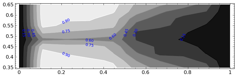
Figure 1: Contour plot of the classification qualities $q(\varphi_{\eta},\mathcal{I}(51,n_{1}))$ of the traffic-majority rules. It shows the fraction of correct classifications for a cellular automaton of ring size $n=51$ that is run for 400 time steps. The horizontal axis is the $\eta$ parameter of the transition rule, and the vertical axis is the initial density $\frac{n_{1}}{n}$ of cells in state 1.

It becomes visible in Figure 1, which shows how the classification quality of $\varphi_{\eta}$ depends on $\eta$ and on the density of the initial configuration.

Another property of the traffic-majority rules that one can see in Figure 1 is the different behaviour of the rule for values less and greater than $\frac{1}{2}$. If $\eta<\frac{1}{2}$, the classification quality is quite good, especially in the interval $0.15<\eta<0.45$, while it becomes bad very fast for $\eta>0.45$: For most densities of ones in an initial configuration, the classification quality is less than $\frac{1}{2}$, which means that in most cases they are not classified correctly.

We can also see in Figure 1 that the classification quality is bad for small $\eta$. The reason for this must be that for small $\eta$ the classification time is very large and the classification process has not finished when the simulation ends. This was already noted by Fatès [4, p. 240].

We will look into all these phenomena in more detail in the following sections, beginning with the symmetry (14) of the transition rule.

3.2 Symmetry

We see from Figure 1 that the classification quality for the initial configuration with density $\frac{n_{1}}{n}$ seems to be the same as that for an initial configuration with density $1-\frac{n_{1}}{n}=\frac{n-n_{1}}{n}$. So it may be that each configuration with $n_{1}$ cells in state 1 corresponds to a configuration with $n-n_{1}$ cells in state 1 that has the same classification quality. The second configuration could be constructed by replacing the cells in state 1 with cells in state 0 and vice versa, but (14) suggests that the order of the cells must be reversed too.

This leads to the following definition, an extension of the notation defined in Definition 5 from numbers to configurations.

Definition 15 (Inverted Configuration).

Let $c\in\mathrm{Conf}(n)$. The inversion of $c$ is the configuration $\bar{c}\in\mathrm{Conf}(n)$ with

$$\bar{c}(x)=\overline{c(n-x)}\qquad\text{for all $x\in\mathbb{Z}_{n}$.}$$ (15)

Let $C\in\mathrm{Conf}(n)^{\Omega}$ be a random variable. The inversion of $C$ is the random variable $\bar{C}\in\mathrm{Conf}(n)$ with

$$\mathbf{P}(\bar{C}=c)=\mathbf{P}(C=\bar{c})\qquad\text{for all $c\in\mathrm{Conf}(n)$.}$$ (16)

We now state the symmetry property in a general form, because we will need it later again for another type of initial conditions.

Lemma 1 (Symmetry).

Let $n\in\mathbb{N}$ and $c\in\mathrm{Conf}(n)$. Then

$$T(\varphi_{\eta},\bar{c})=T(\varphi_{\eta},c)\qquad\text{and}\qquad q(\varphi_{\eta},\bar{c})=q(\varphi_{\eta},c)\,.$$ (17)

Proof.

First we prove that $\Phi_{\eta}(\bar{c})=\overline{\Phi_{\eta}(c)}$ for all $c\in\mathrm{Conf}(n)$. For this, let $x\in\mathbb{Z}_{n}$. Then

$$\mathbf{P}\left(\bigl{(}\overline{\Phi_{\eta}(c)}\bigr{)}(x)=1\right)$$ (18)

$$=\mathbf{P}(\Phi_{\eta}(c)(n-x)=0)$$

$$=\overline{\mathbf{P}(\Phi_{\eta}(c)(n-x)=1)}$$

$$=\overline{\varphi_{\eta}(c(n-x-1),c(n-x),c(n-x+1))}$$

$$=\varphi_{\eta}\bigl{(}\overline{c(n-x+1)},\overline{c(n-x)},\overline{c(n-x-1)}\bigr{)}$$    by (14)

$$=\varphi_{\eta}(\bar{c}(x-1),\bar{c}(x),\bar{c}(x+1))$$

$$=P(\Phi_{\eta}(\bar{c})(x)=1)\,.$$

Then we can show by induction that $\overline{\Phi_{\eta}^{t}(c)}=\Phi_{\eta}^{t}(\bar{c})$ for all $t\geq 0$. From (8) follows $e(\bar{c})=\overline{e(c)}$. Therefore

$$\Phi^{t}(c)=e(c)\quad\text{if and only if}\quad\Phi^{t}(\bar{c})=e(\bar{c})\qquad\text{for all $t\geq 0$.}$$ (19)

Since $T(\varphi,c)=\min\{t\in\mathbb{N}_{0}:\Phi^{t}(c)=e(c)\}$, this proves that $T(\varphi,c)=T(\varphi,\bar{c})$. Since $q(\varphi,c)=\mathbf{P}(q(\varphi,c)\neq\infty)$, this shows also that $q(\varphi,c)=q(\varphi,\bar{c})$. ∎

We will now specialise this theorem to the random initial configurations $\mathcal{I}(n,n_{1})$. The following theorem shows that a random configuration with density $1-\frac{n_{1}}{n}$ has the same classification quality as one with density $\frac{n_{1}}{n}$.

Theorem 1 (Symmetry for $\mathcal{I}(n,n_{1})$).

Let $n\in\mathbb{N}$, $n_{1}\in\mathbb{N}_{0}$ with $n_{1}\leq n$. Then

$$T(\varphi_{\eta},\mathcal{I}(n,n_{1})) =T(\varphi_{\eta},\mathcal{I}(n,n-n_{1})),$$ (20)

$$q(\varphi_{\eta},\mathcal{I}(n,n_{1})) =q(\varphi_{\eta},\mathcal{I}(n,n-n_{1}))\,.$$

Proof.

To apply Lemma 1 we need to prove that $\mathcal{I}(n,n-n_{1})=\overline{\mathcal{I}(n,n_{1})}$.

The proof relies on the symmetry of the binomial coefficient, ${n\choose n-n_{1}}={n\choose n_{1}}$ for $0\leq n_{1}\leq n$, and on the fact that $\#_{1}(c)=n-\#_{1}(\bar{c})$ for all $c\in\mathrm{Conf}(n)$. Then we use (11) to calculate

$$\mathbf{P}(\mathcal{I}(n,n-n_{1})=c) =\frac{[\#_{1}(c)=n-n_{1}]}{{n\choose n-n_{1}}}$$ (21)

$$=\frac{[\#_{1}(\bar{c})=n_{1}]}{{n\choose n_{1}}}$$

$$=\mathbf{P}(\mathcal{I}(n,n_{1})=\bar{c})=\mathbf{P}(\overline{\mathcal{I}(n,n_{1})}=c)\,.$$

This proves that the initial configuration $\mathcal{I}(n,n-n_{1})$ has the same probability distribution as $\overline{\mathcal{I}(n,n_{1})}$. ∎

Theorem 1 allows us to restrict our attention to initial configurations with density less than $\frac{1}{2}$. We will do this in the remaining part of the text.

4 Blocks of Cells in State 1

An analysis of the behaviour of the traffic-majority rule would be very complex if we allowed all elements of $\mathrm{Conf}(n)$ as initial configurations: There is a huge variety of initial configurations, and, since $\varphi_{\eta}$ is non-deterministic, also a huge variety of evolutions for a single initial configuration.

We will therefore now look at one family of initial configurations in more detail, namely those that consist of a block of cells in state 1, surrounded by cells in state 0. We will see that they share a common behaviour.

4.1 Observations

To get a classification quality for blocks we define initial configurations similar to those of Definition 13.

Definition 16 (Blocks as Initial States).

Let $n\in\mathbb{N}_{0}$.

Let $\ell\in\mathbb{N}_{0}$ with $\ell\leq n$. A 1-block of length $\ell$ is a configuration $\mathcal{B}(n,\ell)\in\mathrm{Conf}(n)$ with

$$\mathcal{B}(n,\ell)(x)=[x\in\{0,\dots,\ell-1\}]\qquad\text{for all $x\in\mathbb{Z}_{n}$.}$$ (22)

A random block is a configuration $\mathcal{B}_{n}\in\mathrm{Conf}(n)^{\Omega}$ with

$$\mathbf{P}(\mathcal{B}_{n}=\mathcal{B}(n,\ell))=\frac{1}{n+1}\qquad\text{for all $\ell\in\mathbb{N}_{0}$ with $\ell\leq n$.}$$ (23)

The Block $\mathcal{B}(n,\ell)$ is an initial configuration with density $\frac{\ell}{n}$. Note that in contrast to $\mathcal{I}(n,n_{1})$, it is not a random variable.

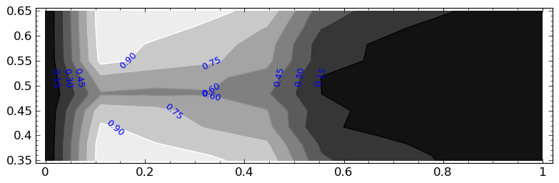
Figure 2: Classification quality for a single block of ones under the traffic-majority rule. The parameters of this contour plot are the same as in Figure 1.

The local classification quality for blocks (Figure 2) has the same general form as that for generic initial conditions; for $\eta>\frac{1}{2}$ it is however even worse. A partial explanation for this behaviour will be given in Section 4.3.

The symmetry property for 1-block initial conditions $\mathcal{B}(n,\ell)$ can now be proved in the same way as that for the generic initial conditions $\mathcal{I}(n,n_{1})$.

Theorem 2 (Symmetry for 1-Blocks).

Let $n\in\mathbb{N}$ and $\ell\in\mathbb{N}_{0}$ with $\ell\leq n$. Then

$$T(\varphi_{\eta},\mathcal{B}(n,\ell)) =T(\varphi_{\eta},\mathcal{B}(n,n-\ell)),$$ (24)

$$q(\varphi_{\eta},\mathcal{B}(n,\ell)) =q(\varphi_{\eta},\mathcal{B}(n,n-\ell))\,.$$

Proof.

We note that $\mathcal{B}(n,n-\ell)=\overline{\mathcal{B}(n,\ell)}$, which can be seen directly from Definition 15 and Equation (22). Therefore we can apply Lemma 1. ∎

4.2 Behaviour of the Boundaries

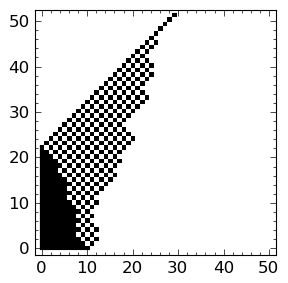
Figure 3: Phases in the development of a block. Phase I ends at time step 21 and Phase II at time step 51.

Now we will look in more details into the evolution of blocks. Figure 3 shows one example, and more samples are given in Figure LABEL:fig:block_samples. In all of them, the initial density is less than $\frac{1}{2}$, so the configurations are supposed to evolve to $e_{0}$.

We can see from these pictures that the repertoire of configurations that occur during the evolution of $\mathcal{B}(n,\ell)$ is limited: They all have the general form $1^{*}(01)^{*}0^{*}$. We now begin with the investigation of the behaviour of these configurations.

As we can see from Figure 3, the evolution of a $\mathcal{B}(n,\ell)$ seems to consist of two phases: one in which a block of consecutive cells in state 1 is present and the other one in which there is only the alternating pattern of 0 and 1.

Definition 17 (Phases).

The time $t$ in the evolution of $\mathcal{B}(n,\ell)$ in which the configuration $\Phi_{\eta}^{t}(\mathcal{B}(n,\ell))$ has the form $11^{*}(10)^{*}0^{*}$, is called Phase I.

The time in which the configuration $\Phi_{\eta}^{t}(\mathcal{B}(n,\ell))$ has the form $(10)^{*}10^{*}$ or a shifted version of it, is Phase II.

In both phases there must be at least one cell in state 1. The end state $e_{0}$ belongs to neither of the phases; we could view it as a third phase.

$\eta=0$	$\eta=0.3$	$\eta=0.5$	$\eta=0.7$	$\eta=1$

The shape of such a configuration is determined by only three numbers. We will work with them instead of cell sequences.

Definition 18 (Boundaries).

Let $(C_{t})_{t\geq 0}=(\Phi_{\eta}^{t}(\mathcal{B}(n,\ell)))_{t\geq 0}$ be the evolution of a 1-block. Let $C_{t}$ be a cell sequence of the form $1^{*}(01)^{*}0^{*}$ in which at least one cell is in state 1.

Now we define $B_{0,t}$, $B_{1,t}$ and $B_{1,t}\in(\mathbb{Z}_{n})^{\Omega}$ in such a way that

1. the region $C_{t}(B_{0,t}),\dots,C_{t}(B_{1,t})$ has the form $11^{*}$,

2. the region $C_{t}(B_{1,t}),\dots,C_{t}(B_{2,t})$ has the form $1(01)^{*}$, and

3. the region $C_{t}(B_{2,t}),\dots,C_{t}(B_{0,t})$ has the form $10^{*}$.

These three random variables are then the boundaries of $C_{t}$. The region between $B_{0,t}$ and $B_{1,t}$ is the 1-block of $C_{t}$ and the region between $B_{1,t}$ and $B_{2,t}$ is the 01-sequence.

We will also use the tuple $\vec{B}_{t}=(B_{0,t},B_{1,t},B_{2,t})$ of the boundaries at time $t$.

The meaning of these three variables is shown in the following diagram:

$$\begin{array}[]{ccccccccccccccccccc}011&1111111111&110&10101010101&010&0\\ \uparrow&&\uparrow&&\uparrow\\ B_{0,t}&&B_{1,t}&&B_{2,t}\end{array}$$ (25)

During Phase I we always have $B_{0,t}\neq B_{1,t}$, and during Phase II there is always $B_{0,t}=B_{1,t}$.

Now we can express the effect of transition rule $\varphi_{\eta}$ on these boundaries. First we introduce a shorter notation for their behaviour in a single time step:

Definition 19 (Single Step Probability).

Let $(b_{0},b_{1},b_{2})$ and $(b^{\prime}_{0},b^{\prime}_{1},b^{\prime}_{2})\in\mathbb{Z}_{n}^{3}$. We define,

$$P(b^{\prime}_{0},b^{\prime}_{1},b^{\prime}_{2}\leftarrow b_{0},b_{1},b_{2})=\mathbf{P}(\vec{B}_{t+1}=(b^{\prime}_{0},b^{\prime}_{1},b^{\prime}_{2})\mid\vec{B}_{t}=(b_{0},b_{1},b_{2}))\,.$$ (26)

Often we will write $P(b^{\prime}_{0},b^{\prime}_{1},b^{\prime}_{2}\leftarrow\vec{b})$ for $P(b^{\prime}_{0},b^{\prime}_{1},b^{\prime}_{2}\leftarrow b_{0},b_{1},b_{2})$.

We will also write $P(e_{0}\leftarrow b_{0},b_{1},b_{2})$ for the probability that the state with boundaries $\vec{B}_{t}=(b_{0},b_{1},b_{2})$ evolves in the next step to $e_{0}$.

If a configuration grows very long during Phase I, it may “wrap around”, such that the right end of the 01-sequence reaches the left end of the 1-block. In this case our model will break down. We can however expect that this kind of behaviour has low probability when the initial 1-block is short enough: such a block is supposed to vanish fast and to stay small while it exists. The examples in Figure LABEL:fig:block_samples support this expectation.

In the following analysis we will therefore assume that the initial 1-block is so short that wrap-arounds are improbable. We will later compare the theoretical results with actual data and find the block lengths for which the assumption is justified.

Theorem 3 (Single Step Behaviour).

Let $b_{2}\neq b_{0}$.

1. Phase I: If $b_{0}\neq b_{1}$, we have the transition probabilities

   $$P(b_{0},b_{1}-1,b_{2}+1 \leftarrow b_{0},b_{1},b_{2}) =\bar{\eta}^{2},$$ (27a)

   $$P(b_{0},b_{1}-1,b_{2}-1 \leftarrow b_{0},b_{1},b_{2}) =\eta\bar{\eta},$$ (27b)

   $$P(b_{0},b_{1}+1,b_{2}+1 \leftarrow b_{0},b_{1},b_{2}) =\eta\bar{\eta},$$ (27c)

   $$P(b_{0},b_{1}+1,b_{2}-1 \leftarrow b_{0},b_{1},b_{2}) =\eta^{2}[b_{1}\neq b_{2}],$$ (27d)

   $$P(b_{0},b_{1},b_{2} \leftarrow b_{0},b_{1},b_{2}) =\eta^{2}[b_{1}=b_{2}]\,.$$ (27e)

   In all other cases, $P(b^{\prime}_{0},b^{\prime}_{1},b^{\prime}_{2}\leftarrow b_{0},b_{1},b_{2})=0$.

2. Phase II: If $b_{0}=b_{1}\neq b_{2}$, we have the transition probabilities

   $$P(b_{1}+1,b_{1}+1,b_{2}+1 \leftarrow b_{1},b_{1},b_{2}) =\bar{\eta},$$ (28a)

   $$P(b_{1}+1,b_{1}+1,b_{2}-1 \leftarrow b_{1},b_{1},b_{2}) =\eta[b_{1}\neq b_{2}],$$ (28b)

   $$P(e_{0} \leftarrow b_{1},b_{1},b_{2}) =\eta[b_{1}=b_{2}]\,.$$ (28c)

   In all other cases, $P(b^{\prime}_{1},b^{\prime}_{1},b^{\prime}_{2}\leftarrow b_{1},b_{1},b_{2})=0$.

Proof.

This is done with the help of diagrams similar to (25).

1. Phase I: Since the probabilities in (27d) and (27e) depend on whether $b_{1}$ and $b_{2}$ are equal or not, we must subdivide Phase I further.

   1. $b_{1}\neq b_{2}$: This is the case where there is both a nontrivial 1-block and a nontrivial 01-sequence. The boundaries $B_{1}$ and $B_{2}$ are separate and move independently to the left and the right.

      $$\begin{array}[]{cccccccc@{\qquad}l@{\quad}l}0&0\underline{1}1&11111111&1\underline{1}0&1010101&0\underline{1}0&0&&b_{0},b_{1},b_{2}\\ \cline{1-7}\cr&011&11111111&1\eta 1&0101010&10\bar{\eta}&\\ \cline{2-6}\cr&0\underline{1}1&11111111&\underline{1}01&0101010&10\underline{1}&&&b_{0},b_{1}-1,b_{2}+1,&p=\bar{\eta}^{2}\\ &0\underline{1}1&11111111&\underline{1}01&0101010&\underline{1}00&&&b_{0},b_{1}-1,b_{2}-1,&p=\bar{\eta}\eta\\ &0\underline{1}1&11111111&11\underline{1}&0101010&10\underline{1}&&&b_{0},b_{1}+1,b_{2}+1,&p=\eta\bar{\eta}\\ &0\underline{1}1&11111111&11\underline{1}&0101010&\underline{1}00&&&b_{0},b_{1}+1,b_{2}-1,&p=\eta^{2}\end{array}$$ (29)

      The left side of this diagram contains partial configurations. Only the 1-block and the 01-sequence is displayed, the surrounding zeros are mostly left out.

      The first line is the initial configuration, with the locations of $B_{0,t}$, $B_{1,t}$ and $B_{2,t}$ underlined. The second line contains for each cell the probability that this cell will be in state 1 at time $t+1$. Most of these probabilities are 0 or 1, which means that the state of this cell is already determined by its neighbourhood at time $t$, but there are two places, $B_{1,t}$ and $B_{2,t}+1$, where randomness enters.

      Since each of these locations may become 0 or 1, there are four possible configurations at time $t+1$. In the last four lines of the diagram they are listed. The second column contains the values for the boundaries $B_{0,t+1}$, $B_{1,t+1}$ and $B_{2,t+1}$ in these configurations, assuming that they had the values $b_{0}$, $b_{1}$ and $b_{2}$ in the previous time step, and the third column has for each configuration the probability that it occurs.

      So in the third line of the diagram we see the first of the possible configurations. In it, $B_{1}$ has moved one place to the left, $B_{2}$ one place to the right, and $B_{0}$ has stayed at 0. This happened because the cell at $B_{1,t}$, which could stay in state state 1 with probability $\eta$, has switched to state 0, and the cell at $B_{2,t}+1$ has switched to state 1. Both events are independent and have probability $\bar{\eta}$, so the probability for the whole configuration is $\bar{\eta}^{2}$. This proves (27a) in case of $b_{1}\neq b_{2}$, and the other lines of (27) are proved similarly.

      These four cases are the only possible configurations for the next time step, therefore all other transitions must have probability 0.

   2. $b_{1}=b_{2}$: Since $b_{0}=0$, this configuration is a $\mathcal{B}(n,b_{1}+1)$ for some $n>b_{1}+1$.

      $$\begin{array}[]{cccccc@{\qquad}l@{\quad}l}0&0\underline{1}1&1111111111&1\underline{\underline{1}}0&0&&b_{0},b_{1},b_{1}\\ \cline{1-5}\cr&011&1111111111&1\eta\bar{\eta}\\ \cline{2-4}\cr&0\underline{1}1&1111111111&\underline{1}0\underline{1}&&&b_{0},b_{1}-1,b_{1}+1,&p=\bar{\eta}^{2}\\ &0\underline{1}1&1111111111&\underline{\underline{1}}00&&&b_{0},b_{1}-1,b_{1}-1,&p=\bar{\eta}\eta\\ &0\underline{1}1&1111111111&11\underline{\underline{1}}&&&b_{0},b_{1}+1,b_{1}+1,&p=\eta\bar{\eta}\\ &0\underline{1}1&1111111111&1\underline{\underline{1}}0&&&b_{0},b_{1},b_{1},&p=\eta^{2}\end{array}$$ (30)

      When $B_{1}$ and $B_{2}$ have the same value, their place is marked by a double underlining.

2. Phase II: This is a pure 01-sequence. The left side always moves to the right, and the only place where randomness enters is the right side. Here there are only two possibilities: either the length of the sequence stays the same or it shrinks.

   A special case occurs when $b_{0}=b_{2}$. Then we have a configuration with exactly one cell in state 1. and it may vanish altogether; then the classification process has finished.

   We have therefore again two cases.

   1. $b_{0}\neq b_{2}$:

      $$\begin{array}[]{cccccc@{\qquad}l@{\quad}l}0&\underline{\underline{1}}0&10101010101&0\underline{1}0&0&&b_{0},b_{0},b_{2}\\ \cline{1-5}\cr&01&01010101010&10\bar{\eta}&\\ \cline{2-4}\cr&0\underline{\underline{1}}&01010101010&10\underline{1}&&&b_{0}+1,b_{0}+1,b_{2}+1,&p=\bar{\eta}\\ &0\underline{\underline{1}}&01010101010&\underline{1}00&&&b_{0}+1,b_{0}+1,b_{2}-1,&p=\eta\end{array}$$ (31)

   2. $b_{0}=b_{2}$:

      $$\begin{array}[]{cccc@{\qquad}l@{\quad}l}0&\underline{\underline{\underline{1}}}0&0&&b_{0},b_{0},b_{0}\\ \cline{1-3}\cr&0\bar{\eta}&\\ \cline{2-2}\cr&0\underline{\underline{\underline{1}}}&&&b_{0}+1,b_{0}+1,b_{o}+1,&p=\bar{\eta}\\ &00&&&e_{0},&p=\eta\end{array}$$ (32)

∎

The theorem allows to conclude that Phase I and Phase II do occur in this order in the evolution of a $\mathcal{B}(n,\ell)$. This is because the initial configuration belongs to Phase I and, as long as no wraparound occurs, the successor of a Phase I configuration belongs either to Phase I or Phase II. The change between the phases can only occur if $b_{0}+1=b_{1}$, as a special case of (27a) or (27b). The transitions of Phase II then either preserve the property $b_{0}=b_{1}$ that defines this phase, or they lead to the end configuration $e_{0}$.

4.3 Global Classification Quality for 1-Blocks

We must find out how useful 1-blocks are as an estimate for the behaviour of all initial conditions.

In this section we will look at this question in terms of the global classification quality.

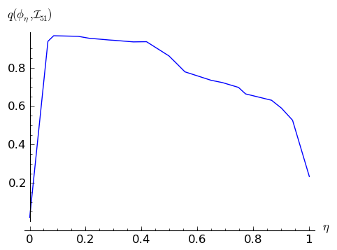
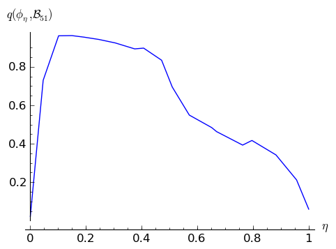
Figure 5: Classification quality of the traffic-majority rule on 51 cells for different values of $\eta$, with generic initial configurations (left) and with 1-blocks (right). The simulations were run for at most 400 time steps and repeated 1000 times for each value of $\eta$, each time with a random initial configuration.

The empirical values are shown in Figure 5. We see that for $\eta<\frac{1}{2}$ the global classification quality $q(\varphi_{\eta},\mathcal{I}_{n})$ is very good, larger that $0.9$, and that it is almost as good when restricted to 1-blocks. For $\eta\geq\frac{1}{2}$, the generic classification quality $q(\varphi_{\eta},\mathcal{I}_{n})$ becomes worse, falling almost monotonously with rising $\eta$. A qualitative change occurs near $\eta=\frac{1}{2}$, as in Figure 1.

The same effect is visible for 1-block initial conditions, but it is even stronger. For $\eta<\frac{1}{2}$, the 1-blocks behave similar to generic initial configurations, while for higher values they behave worse. One cause for this is a theorem about archipelagos proved by Fatès [3].

Definition 20 (Archipelago [3, p. 286]).

Let $\sigma\in\Sigma$. A configuration $c\in\mathrm{Conf}(n)$ is a $\sigma$-archipelago if all cells in state $\sigma$ are isolated, i. e. if there is no $x\in\mathbb{Z}_{n}$ with $c(x)=c(x+1)=\sigma$.

Theorem 4.

If $0\leq\eta<1$, then the transition rule $\varphi_{\eta}$ classifies all $\sigma$-archipelagos correctly.

Proof.

This is [3, Lemma 4]. The condition on $\eta$ is not explicitly stated there, but it follows from the proof. ∎

The intersection between the sets of archipelagos and that of 1-blocks is very small: $\mathcal{B}(n,0)=e_{0}$ and $\mathcal{B}(n,n-1)$ are 0-archipelagos, while $\mathcal{B}(n,n)=e_{1}$ and $\mathcal{B}(n,1)$ are 1-archipelagos. All other archipelagos can occur only as random configurations $\mathcal{I}_{n}$.

Now we can understand why the classification quality is higher for random initial configurations than for blocks if $\eta>\frac{1}{2}$. For these values of $\eta$, the classification quality is rather bad, as we have seen. However, the low classification quality of $\varphi_{\eta}$ does not affect initial configurations that are archipelagos. This effect influences $\mathcal{I}_{n}$ initial configurations with a higher probability than block initial configurations, and therefore the classification quality for $\mathcal{I}_{n}$ is better.

4.4 Deterministic Classification

For block initial conditions and $\eta\in\{0,1\}$ we can show that the only 1-blocks that are classified correctly are the four archipelago configuration described before. For these initial configurations we can therefore actually compute the classification quality for $\varphi_{\eta}$:

Theorem 5 (Block Classification in the Deterministic Cases).

Let $n>1$ be odd. Then

$$q(\varphi_{0},\mathcal{B}_{n})=\frac{4}{n}\qquad\text{and}\qquad q(\varphi_{1},\mathcal{B}_{n})=\frac{2}{n}\,.$$ (33)

Proof.

We know already that $\mathcal{B}(n,0)$, $\mathcal{B}(n,1)$, $\mathcal{B}(n,n-1)$ and $\mathcal{B}(n,n)$ are always classified correctly by the rule $\varphi_{0}$. For $\varphi_{1}$, the Archipelago Theorem does not apply, but $e_{0}$ and $e_{1}$ are trivially classified correctly. If these are the only 1-blocks that are classified correctly, the formulas in (33) follow. It remains therefore to prove that no other 1-block is classified correctly.

We must then look at the evolution of $\mathcal{B}(n,\ell)$ for the values of $\ell$ for which correct classification has not been proved. Because of the symmetry of $\varphi_{\eta}$ (Theorem 2) we only need to consider the case of $\ell\leq\frac{n}{2}$. In this case a correct classification takes place if there is a time at which the automaton is in configuration $e_{0}$.

The following two lemmas describe the evolution of $\mathcal{B}(n,\ell)$ for $\eta=0$ and $\eta=1$. They show that in both cases the configuration evolves to a state that stays essentially unchanged over time and is always different from $e(\mathcal{B}(n,\ell))$: no classification occurs, and the theorem is true. ∎

The evolution of a $\mathcal{B}(n,\ell)$ under $\eta=0$ is shown in the left column of Figure LABEL:fig:block_samples.

Lemma 2 (Block Evolution for $\eta=0$).

Let $2\leq\ell<\frac{n}{2}$. Then an evolution under $\varphi_{0}$ starting from $\mathcal{B}(n,\ell)$ has for $0\leq t\leq\ell-1$,

$$B_{0,t} =0,\quad B_{1,t}=\ell-1-t, B_{2,t} =\ell-1+t$$ (34a)

and for $$t\geq\ell-1$$,

$$B_{0,t} =B_{1,t}=t-\ell-1, B_{2,t} =\ell-1+t\,.$$ (34b)

A correct classification never occurs.

Proof.

At time $t=0$ the boundaries of a $\mathcal{B}(n,\ell)$ are $B_{0,0}=0$ and $B_{1,0}=B_{2,0}=\ell-1$. We have $B_{0,0}\neq B_{1,0}$ because of $\ell\geq 2$ and are therefore in Phase I.

Among the transitions with nonzero probability in Theorem 3, only (27a) and (28a) are important here. For $\eta=0$, they become

$$P(b_{0},b_{1}-1,b_{2}+1 \leftarrow\vec{b}) =[b_{0}\neq b_{1}],$$ (35a)

$$P(b_{1}+1,b_{1}+1,b_{2}+1 \leftarrow b_{1},b_{1},b_{2}) =[b_{1}\neq b_{2}]\,.$$ (35b)

At the beginning, with $B_{0,0}\neq B_{1,0}$, transition (35a) has a nonzero probability. Therefore $B_{0,1}=B_{0,0}$, $B_{1,1}=B_{1,0}-1=\ell-2$ and $B_{2,1}=B_{2,0}+1=\ell$. So $B_{1}$ has moved one location to the left and $B_{2}$ has moved one location to the right. This process goes on for $\ell$ time steps, from $t=0$ to $t=\ell-1$. In all of them we have $B_{0,t}=0$, $B_{1,t}=\ell-1-t$ and $B_{2,t}=\ell-1+t$. This proves (34a).

At time $\ell$ we have $B_{0,\ell-1}=B_{1,\ell-1}=0$ and $B_{2,\ell-1}=2\ell-1$. The configuration of the automaton then contains a sequence $1010101\dots 01$ reaching from 0 to $2\ell-1$.

Because $\ell<\frac{n}{2}$, this structure has not yet wrapped around the ring of cells. In fact, since $n$ is odd, we must have $2\ell\leq n-1$ and there is a gap of at least two cells in state 0 between $B_{2,\ell-1}=2\ell-1$ and $B_{0,\ell-1}=0$.

This becomes important for times later than $\ell-1$. Phase I has ended then, and now the process described in (35b) has nonzero probability. This means that $B_{0,t+1}=B_{0,t}+1$, $B_{1,t+1}=B_{1,t}+1$ and $B_{2,t+1}=B_{2,t}+1$, so the $01$-sequence moves with every time step one location to the right in the cyclic structure of the cellular automaton, a process that never ends. Especially the configuration $e_{0}$ never occurs. The values of $\vec{B}_{t}$ for this phase are given in (34b). ∎

The evolution of a $\mathcal{B}(n,\ell)$ under $\eta=1$ is shown in the right column of Figure LABEL:fig:block_samples.

Lemma 3 (Block Evolution for $\eta=1$).

Let $1\leq\ell\leq\frac{n}{2}$. Then an evolution under $\varphi_{1}$ starting from $\mathcal{B}(n,\ell)$ has for all $t\geq 0$,

$$B_{0,t}=0,\quad B_{1,t}=\ell-1,\quad B_{2,t}=\ell-1\,.$$ (36)

A correct classification never occurs.

Proof.

At time $t=0$, the boundaries of a $\mathcal{B}(n,\ell)$ are $B_{0,0}=0$ and $B_{1,0}=B_{2,0}=\ell-1$.

Among the processes of Theorem 3 with nonzero probability, only process (27e) is important for $\eta=1$; it becomes

$$P(b_{0},b_{1},b_{2} \leftarrow\vec{b}) =[b_{1}=b_{2}]\,.$$ (37)

This means that $B_{t}$ never changes: the initial configuration stays the same and never becomes $e_{0}$. ∎

For $n=51$, Theorem 5 implies that $q(\varphi_{0},\mathcal{B}_{n})\approx 0.078$ and $q(\varphi_{1},\mathcal{B}_{n})\approx 0.039$. This agrees with Figure 5.

5 Approximation by Random Walks

5.1 The Model

In this section we introduce a simplified model for the behaviour of the boundaries of the 01-block, $B_{1,t}$ and $B_{2,t}$. In the model, we assume that they are independent random variables, each performing a random walk. We expect it to be valid if the initial configuration is a $\mathcal{B}(n,\ell)$ for which $\ell$ is small in comparison to $n$ and if the transition rule $\varphi_{\eta}$ has $\eta<\frac{1}{2}$.

The model is motivated by the following lemma: It shows that if $B_{1,t}$ and $B_{2,t}$ are distinct, they indeed behave independently.

Lemma 4 (Boundary Independence).

In Phase I, if $B_{0,t}\neq B_{1,t}\neq B_{2,t}$, then $B_{1,t+1}$ and $B_{2,t+1}$ are stochastically independent with the conditional probabilities

$$\mathbf{P}(B_{1,t+1}=x\mid B_{1,t}=b_{1}) =[x=b_{1}-1]\bar{\eta}+[x=b_{1}+1]\eta,$$ (38a)

$$\mathbf{P}(B_{2,t+1}=x\mid B_{2,t}=b_{2}) =[x=b_{2}-1]\eta+[x=b_{2}+1]\bar{\eta}\,.$$ (38b)

In Phase II, if $B_{1,t}\neq B_{2,t}$, equation (38b) is valid too.

Proof.

Let $B_{i,t}=b_{i}$ for $i=0,1,2$. Then, in Phase I,

$$\mathbf{P}(B_{1,t+1}=b_{1}-1\mid\vec{B}_{t}=\vec{b}) =\sum_{b^{\prime}_{0}\in\mathbb{Z}}\sum_{b^{\prime}_{2}\in\mathbb{Z}}P(b^{\prime}_{0},b_{1}-1,b^{\prime}_{2}\leftarrow\vec{b})$$

$$=P(b_{0},b_{1}-1,b_{2}-1\leftarrow\vec{b})$$

$$\quad+P(b_{0},b_{1}-1,b_{2}+1\leftarrow\vec{b})$$

$$=\bar{\eta}^{2}+\eta\bar{\eta}=\bar{\eta},$$ (39a)

$$\mathbf{P}(B_{1,t+1}=b_{1}+1\mid\vec{B}_{t}=\vec{b}) =\sum_{b^{\prime}_{0}\in\mathbb{Z}}\sum_{b^{\prime}_{2}\in\mathbb{Z}}P(b^{\prime}_{0},b_{1}+1,b^{\prime}_{2}\leftarrow\vec{b})$$

$$=P(b_{0},b_{1}+1,b_{2}-1\leftarrow\vec{b})$$

$$\quad+P(b_{0},b_{1}+1,b_{2}+1\leftarrow\vec{b})$$

$$=\eta\bar{\eta}+\eta^{2}=\eta,$$ (39b)

which proves (38a). In a similar way we prove (38b) with the calculations

$$\mathbf{P}(B_{2,t+1}=b_{2}-1\mid\vec{B}_{t}=\vec{b}) =P(b_{0},b_{1}-1,b_{2}-1\leftarrow\vec{b})$$

$$\quad+P(b_{0},b_{1}+1,b_{2}-1\leftarrow\vec{b})$$

$$=\bar{\eta}\eta+\eta^{2}=\eta,$$ (40a)

$$\mathbf{P}(B_{2,t+1}=b_{2}+1\mid\vec{B}_{t}=\vec{b}) =P(b_{0},b_{1}-1,b_{2}+1\leftarrow\vec{b})$$

$$\quad+P(b_{0},b_{1}+1,b_{2}+1\leftarrow\vec{b})$$

$$=\bar{\eta}^{2}+\eta\bar{\eta}=\bar{\eta}\,.$$ (40b)

In Phase II, we must apply equations (28). Here we have in both cases only one summand, and the computations are

$$\mathbf{P}(B_{2,t+1}=b_{2}-1 \mid\vec{B}_{t}=\vec{b})$$

$$=P(b_{1}+1,b_{1}+1,b_{2}-1\leftarrow b_{1},b_{1},b_{2})=\eta,$$ (41a)

$$\mathbf{P}(B_{2,t+1}=b_{2}+1 \mid\vec{B}_{t}=\vec{b})$$

$$=P(b_{1}+1,b_{1}+1,b_{2}+1\leftarrow b_{1},b_{1},b_{2})=\bar{\eta}\,.$$ (41b)

∎

Now a few words about the heuristic justification for the model: We can see from the examples in the second column of Figure LABEL:fig:block_samples that, when the boundaries of the 01-block have separated, they stay so for a long time. This is an experimental justification for the model. A more convincing argument uses equations (38). They show that $B_{1,t}$ tends to move to the left and $B_{2,t}$ to the right if $\eta<\frac{1}{2}$. Their movements are symmetric, which means that when $B_{1,t}=0$ and Phase I ends, $B_{2,t}$ must have moved approximately $\ell$ positions to the right. So if $\ell$ is much smaller than $\frac{n}{2}$, there is only a low probability that a wraparound occurs, the other condition that this model could break down. Therefore it is a good approximation for Phase I if $\eta$ and $\ell$ are small.

There is no danger of a wraparound in Phase II, so the model is also applicable to it.

5.2 Random Walks

We will now introduce some terminology for random walks. The random walks used here may have an end, and this becomes part of their definition. We will also need to specify the way that the random walker has taken, something I have called here its path.

Definition 21 (Paths and Random Walks).

A path through $\mathbb{Z}$ is a pair $(s_{x},x)$ with $s_{x}\in\mathbb{N}_{0}\cup\{\infty\}$ and $x=(x_{t})_{0\leq t\leq s_{x}}$ a sequence of elements of $\mathbb{Z}$. The number $s_{x}$ is the stopping time of $x$. We will usually speak of “the path $x$” when meaning $(s_{x},x)$. The set of all paths is $\Pi$.

A bounded random walk is a random variable with values in $\Pi$.

Let $p\in[0,1]$. A $p$-walk $(s_{X},X)\in\Pi^{\Omega}$ is a bounded random walk with the property that for all $t$ with $0\leq t\leq s_{x}$,

$$\mathbf{P}(X_{t+1}=x+1\mid X_{t}=x) =p,$$ (42a)

$$\mathbf{P}(X_{t+1}=x-1\mid X_{t}=x) =\bar{p}\,.$$ (42b)

We will now translate the movement of the terms $B_{i,t}$ into the language of bounded random walks. This is necessary because we will later use results about random walks in $\mathbb{Z}$, but the boundary terms have values in $\mathbb{Z}_{n}$. The stopping times of the new random walks will also have a useful interpretation.

In order to simplify the computations below, we now artificially extend the domain of $B_{2,t}$ to the first time step at which the automaton is in state $e_{0}$. For this, let $t_{e}$ be the first time at which the automaton is in state $e_{0}$. We will then set $B_{2,t_{e}}=B_{2,t_{e}-1}-1$. We assume thus that at the end of Phase II, the boundary $B_{2}$ takes one final step to the left.

Definition 22 (Boundary Walks).

Let $1\leq\ell\leq\frac{n}{2}$.

Let $(C_{t})_{t\geq 0}=(\Phi_{\eta}^{t}(\mathcal{B}(n,\ell)))_{t\geq 0}$ be the evolution of a 1-block.

Let $B^{\mathbb{Z}}_{1}$ and $B^{\mathbb{Z}}_{2}$ be the bounded random walks with the properties:

1. The stopping time $s_{B^{\mathbb{Z}}_{1}}$ is the first time at which $B_{1,t}=0$, while $s_{B^{\mathbb{Z}}_{2}}=T(\varphi_{\eta},\mathcal{B}(n,\ell))$.

   If however a wraparound occurs during Phase I, i. e. if there is a time $t$ with $B_{0,t}\neq B_{1,t}$ and $B_{2,t}=n-2$, then $s_{B^{\mathbb{Z}}_{1}}=s_{B^{\mathbb{Z}}_{2}}=0$.

2. For $i=1$, $2$ we have

   $$B^{\mathbb{Z}}_{i,0} =B_{i,0},$$ (43a)

   $$B^{\mathbb{Z}}_{i,t}\bmod n =B_{i,t} 0\leq t\leq s_{B^{\mathbb{Z}}_{i}}$$ for , (43b)

   $$\mathopen{|}B^{\mathbb{Z}}_{i,t+1}-B^{\mathbb{Z}}_{i,t}\mathclose{|} \leq 1 0\leq t<s_{B^{\mathbb{Z}}_{i}}$$ for . (43c)

Then the boundary walks for $\mathcal{B}(n,\ell)$ are the pair $\vec{B}^{\mathbb{Z}}=(B^{\mathbb{Z}}_{1},B^{\mathbb{Z}}_{2})$ of bounded random walks.

We know from Theorem 3 that (43c) can always be fulfilled, therefore $\vec{B}^{\mathbb{Z}}$ exists for every $\mathcal{B}(n,\ell)$. The definition of the stopping times means that $s_{B^{\mathbb{Z}}_{1}}$ is the first time step after Phase I and $s_{B^{\mathbb{Z}}_{2}}$ is the first time step after Phase II.

The following lemma shows another way to characterise $s_{B^{\mathbb{Z}}_{2}}$. It will be needed for the simplified model.

Lemma 5 (Stopping Time).

The stopping time $s_{B^{\mathbb{Z}}_{2}}$ is the smallest value of $t$ for which $t-B^{\mathbb{Z}}_{2,t}=s_{B^{\mathbb{Z}}_{1}}+2$.

Proof.

Let $t_{e}=s_{B^{\mathbb{Z}}_{2}}$ be the end time of the classification.

Let $\beta(t)=\max\{0,t-s_{B^{\mathbb{Z}}_{1}}\}$ be the number of time steps since the end of Phase I. During Phase I, $B_{0}$ stays at location 0, while at every time step of Phase II, $B_{0}$ moves one location to the right. Therefore $B_{0,t}=\beta(t)\bmod n$ for all $t<t_{e}$.

Since $B_{0,t}$ is always at the left of $B_{2,t}$, we must have $\beta(t)\leq B^{\mathbb{Z}}_{2,t}$ for all $t<t_{e}$. At time $t_{e}-1$, the configuration consists of exactly one cell in state 1, therefore $\beta(t_{e}-1)=B^{\mathbb{Z}}_{2,t_{e}-1}$. Since $\beta(t_{e})=\beta(t_{e}-1)+1$ and $B^{\mathbb{Z}}_{2,t_{e}}=B^{\mathbb{Z}}_{2,t_{e}-1}-1$, we must have $\beta(t_{e})-1=B^{\mathbb{Z}}_{2,t_{e}}+1$. On the other hand, $t_{e}>s_{B^{\mathbb{Z}}_{1}}$ and therefore $\beta(t_{e})=t-s_{B^{\mathbb{Z}}_{1}}$, so we must have $t-s_{B^{\mathbb{Z}}_{1}}-1=B^{\mathbb{Z}}_{2,t_{e}}+1$, which proves the lemma. ∎

Now, to express the content of Lemma 4 in the language of $p$-walks, we introduce a definition that expresses the restrictions used in that theorem.

Definition 23.

Let $N\in\Pi^{2}$ the set of non-crossing path pairs,

$$N=\{\,(x_{1},x_{2})\in\Pi^{2}:s_{x_{1}}\leq s_{x_{2}},\\ \forall t\in\{1,\dots,s_{x_{1}}\}\colon 0\leq x_{1,t}<x_{2,t}\leq n-2\,\}$$ (44)

Then we can say that if $\vec{B}^{\mathbb{Z}}\in N$, then $B^{\mathbb{Z}}_{1}$ has the transition probabilities of an $\eta$-walk and $B^{\mathbb{Z}}_{2}$ has the transition probabilities of an $\bar{\eta}$-walk, i. e.

$$\mathbf{P}(B^{\mathbb{Z}}_{1,t+1}=x\mid B^{\mathbb{Z}}_{1,t}=b_{1}) =[x=b_{1}-1]\bar{\eta}+[x=b_{1}+1]\eta,$$ (45a)

$$\mathbf{P}(B^{\mathbb{Z}}_{2,t+1}=x\mid B^{\mathbb{Z}}_{2,t}=b_{2}) =[x=b_{2}-1]\eta+[x=b_{2}+1]\bar{\eta}\,.$$ (45b)

This is Lemma 4, translated into the language of bounded random walks.

The simplified model then consists only of $p$-walks.

Definition 24 (Approximation by Random Walks).

Let $\ell\in\mathbb{N}$ and $A_{1}$, $A_{2}\in\Pi^{\Omega}$ be two bounded random walks that start at $\ell-1$.

Let $A_{1}$ be an $\eta$-walk that ends at the first time $t$ with $A_{1,t}=0$.

Let $A_{2}$ be an $\bar{\eta}$-walk that ends at the first time $t$ with $t-A_{2,t}=s_{A_{1}}+2$.

Then the pair $\vec{A}=(A_{1},A_{2})$ is the approximation for $\vec{B}$ with block length $\ell$.

In this model, $A_{1}$ simulates $B^{\mathbb{Z}}_{1}$ during Phase I and at the first time step of Phase II, and $A_{2}$ simulates $B^{\mathbb{Z}}_{2}$ during both phases and the additional time step added for Definition 22. Therefore $s_{A_{1}}$ stands for the time Phase II begins and $s_{A_{2}}$ for the classification time. The characterisation of $s_{A_{2}}$ follows from Lemma 5.

To justify the definition we note that if $\vec{x}\in N$, then $\mathbf{P}(\vec{A}=\vec{x})=\mathbf{P}(\vec{B}^{\mathbb{Z}}=\vec{x})$: every step in $x$ has the same probability under $\vec{A}$ as under $\vec{B}^{\mathbb{Z}}$. So the simplified model and $\vec{B}^{\mathbb{Z}}$ assign the same probabilities to paths in $N$. They may however differ on the rest of the paths.

To investigate the effect of the approximation to the classification problem we now look at $\mathbf{P}(s_{B_{2}}=t_{2})$, the probability that a classification required exactly $t_{2}$ steps. If we know this probability for all $t_{2}$, we know $T(\varphi_{\eta},\mathcal{B}(n,\ell))$ and therefore also $q(\varphi_{\eta},\mathcal{B}(n,\ell))$. In the unapproximated case we can split the probability in the following way,

$$\mathbf{P}(s_{B_{2}}=t_{2}) =\mathbf{P}(s_{B_{2}}=t_{2},\vec{B}^{\mathbb{Z}}\in N)+\mathbf{P}(s_{B_{2}}=t_{2},\vec{B}^{\mathbb{Z}}\notin N)$$ (46)

and we will do the same thing for the approximation,

$$\mathbf{P}(s_{A_{2}}=t_{2}) =\mathbf{P}(s_{A_{2}}=t_{2},\vec{A}\in N)+\mathbf{P}(s_{A_{2}}=t_{2},\vec{A}\notin N)\,.$$ (47)

A measure for the quality of the approximation is the difference between the two probabilities. We know that $\mathbf{P}(s_{B_{2}}=t_{2},\vec{B}^{\mathbb{Z}}\in N)=\mathbf{P}(s_{A_{2}}=t_{2},\vec{A}\in N)$, because there are again only path pairs involved with the same probability under $\vec{B}^{\mathbb{Z}}$ and under $\vec{A}$, and therefore

$$\mathopen{|}\mathbf{P}(s_{B_{2}}=t_{2})-\mathbf{P}(s_{A_{2}}=t_{2})\mathclose{|}\\ =\mathopen{|}\mathbf{P}(s_{B_{2}}=t_{2},\vec{B}^{\mathbb{Z}}\notin N)-\mathbf{P}(s_{A_{2}}=t_{2},\vec{A}\notin N)\mathclose{|}\,.$$ (48)

If this difference is small, then the approximation of $\vec{B}^{\mathbb{Z}}$ by $\vec{A}$ is good.

We know from the proof of Lemma 2 that for $\eta=0$, all possible values of $\vec{B}^{\mathbb{Z}}$ are elements of $N$. Therefore the difference (48) is 0 in this case. Since the probability $\mathbf{P}(s_{B^{\mathbb{Z}}_{2}}=t_{2},\vec{B}^{\mathbb{Z}}\in N)$ varies continuously with $\eta$, we can expect that the approximation becomes better as $\eta$ approaches 0. The probability for a wraparound during Phase I becomes smaller when $\ell$ is small in comparison to $n$. So we should expect a good approximation if $\eta\approx 0$ and $\frac{\ell}{n}$ is not too large.

What these vague conditions actually mean, we will now find out by experiment. We will now derive the classification quality and time for the approximation and then compare it with empirical values.

5.3 Generating Functions

We will use generating functions [9, Definition 5.1.8] for the random walk computations.

Definition 25 (Generating Function).

Let $X\in(\mathbb{N}_{0}\cup\{\infty\})^{\Omega}$ be a random variable. The generating function for $X$ is the function

$$G_{X}(s)=\mathbf{E}(s^{X})=\sum_{k\geq 0}\mathbf{P}(X=k)s^{k}\,.$$ (49)

Generating functions can be used to find the expected values of random variables.

Theorem 6 (Properties of Generating Functions).

Let $X\in(\mathbb{N}_{0}\cup\{\infty\})^{\Omega}$ be a random variable. Then

$$G_{X}(1)=\mathbf{P}(X\neq\infty)\,.$$ (50)

If $G_{X}(1)=1$, then

$$G_{X}^{\prime}(1)=\mathbf{E}(X).$$ (51)

Proof.

These are Theorem 5.1.10 and formula (5.1.20) of [9]. ∎

In the context of stochastic processes with discrete time, $G_{X}(1)$ has a more concrete interpretation. Here, “$X=k$” is interpreted as, “Event $X$ happens at time $k$”, and $X$ is an event that occurs at most once in the duration of the process. If event $X$ never happens, the random variable $X$ has the value $\infty$, and therefore $G_{X}(1)$ is the probability that event $X$ happens at all.

The generating functions that we will use here will have other parameters beside $s$, but the derivatives we will need will be always with respect to $s$; therefore the following convention will make formulas easier to read:

Definition 26 (Convention about Derivatives).

In a generating function with several parameters, like $F_{-1}(p,s)$ below, the derivative $F_{-1}^{\prime}$ is always with respect to $s$: We have $F_{-1}^{\prime}(p,s)=\frac{d}{ds}F_{-1}(p,s)$.

Another method to avoid a cumbersome notation is the use of special names for the generating functions for $s_{A_{1}}$ and $s_{A_{2}}$.

Definition 27 (Generating Functions for the Ends of Phase I and II).

Let $\vec{A}$ be an approximation with block length $\ell$.

Then $G_{I}(\ell,s)$ is the generating function for $s_{A_{1}}$ and $G_{II}(\ell,s)$ is the generating function for $s_{A_{2}}$.

5.4 Computation of the Expected End Time

Our next task will be to find these functions. $G_{I}$ is actually well-known:

Lemma 6 (Reaching 0).

The generating function for the first time $t$ at which a $p$-walk starting from 0 reaches $X_{t}=0$ again is

$$F_{0}(p,s)=1-\sqrt{1-4p\bar{p}s^{2}}\,.$$ (52)

The generating function for the first time a $p$-walk starting from 1 reaches 0 is

$$F_{-1}(p,s)=\frac{F_{0}(p,s)}{2ps}\,.$$ (53)

The generating function for the first time a $p$-walk starting from $n\in\mathbb{N}$ reaches 0 is

$$F_{-n}(p,s)=F_{-1}(p,s)^{n}\,.$$ (54)

Proof.

This are Theorems 5.3.1 and 5.3.5 of [9]. Instead of (53) and (54) they have formulas for $F_{1}$ and $F_{n}$; but the formulas here can be easily derived by noting that $F_{-n}(p,s)=F_{n}(\bar{p},s)$. ∎

The following lemma helps us to compute properties of $F_{-1}$, which in turn will be used for $G_{II}$.

Lemma 7 (Values of $F_{-1}$).

$$F_{-1}(p,1) =\frac{\min\{p,\bar{p}\}}{p},$$ (55a)

$$F_{-1}^{\prime}(p,1) =\frac{2\bar{p}}{1-2\min\{p,\bar{p}\}}-\frac{\min\{p,\bar{p}\}}{p}\,.$$ (55b)

If $$p\leq\frac{1}{2}$$, this becomes

$$F_{-1}(p,1) =1,$$ (55c)

$$F_{-1}^{\prime}(p,1) =\frac{1}{1-2p}\,.$$ (55d)

Proof.

A useful formula for the following calculations is

$$\sqrt{1-4p\bar{p}}=1-2\min\{p,\bar{p}\}\,.$$ (56)

To prove it we note that $\sqrt{1-4p\bar{p}}=\sqrt{1-4p+4p^{2}}=\sqrt{(1-2p)^{2}}=\mathopen{|}1-2p\mathclose{|}$. If $p\leq\bar{p}$, then $p\leq\frac{1}{2}$ and therefore $\mathopen{|}1-2p\mathclose{|}=1-2p=1-2\min\{p,\bar{p}\}$. Since $\sqrt{1-4p\bar{p}}$ is symmetric in $p$ and $\bar{p}$, the same argument is valid for $\bar{p}\leq p$. This proves (56).

With (56) we can compute $F_{-1}(p,1)$:

$$F_{0}(p,1) =1-\sqrt{1-4p\bar{p}}=2\min\{p,\bar{p}\},$$ (57)

$$F_{-1}(p,1) =\frac{F_{0}(p,1)}{2p}=\frac{\min\{p,\bar{p}\}}{p}\,.$$ (58)

From this we see that if $p\leq\frac{1}{2}$ then $F_{-1}(p,1)=1$.

For the computation of $F_{-1}^{\prime}(p,1)$ we start with the derivative of $F_{0}$.

$$F_{0}^{\prime}(p,s) =-\frac{1}{2\sqrt{1-4p\bar{p}s^{2}}}(-4p\bar{p}\cdot 2s)=\frac{4p\bar{p}s}{\sqrt{1-4p\bar{p}s^{2}}}\,.$$ (59)

Next we note that the formula for the derivative of a quotient can be written in the form $\left(\frac{f}{g}\right)^{\prime}=\frac{f^{\prime}}{g}-\left(\frac{f}{g}\right)\frac{g^{\prime}}{g}$. This leads to

$$F_{-1}^{\prime}(p,s)=\frac{F_{0}^{\prime}(p,s)}{2ps}-F_{-1}(p,s)\frac{2p}{2ps}=\frac{2\bar{p}}{\sqrt{1-4p\bar{p}s^{2}}}-\frac{F_{-1}(p,s)}{s}\,.$$ (60)

In case of $s=1$ this becomes

$$F_{-1}^{\prime}(p,1)=\frac{2\bar{p}}{1-2\min\{p,\bar{p}\}}-\frac{\min\{p,\bar{p}\}}{p},$$ (61)

and if $p\leq\frac{1}{2}$,

$$F_{-1}^{\prime}(p,1)=\frac{\bar{p}}{1-2p}-1=\frac{2-2p}{1-2p}-1=\frac{1}{1-2p}\,.$$ (62)

∎

Since $A_{1}$ is an $\eta$-walk starting from $\ell-1$ and ending at the time $t$ at which $A_{1,t}=0$, the generating function for its end time $s_{A_{1}}$ is

$$G_{I}(\ell,p)=F_{-(\ell-1)}(\eta,s)=F_{-1}(\eta,s)^{\ell-1}$$ (63)

The last equality follows from (54).

The stopping condition for $A_{2}$ is expressed in Definition 24 in terms of the difference $t-A_{2,t}$, not of $A_{2,t}$. To speak about paths with such a stopping condition we now define a function $D\colon\Pi\to\Pi$, which maps a path $x$ to the path

$$D(x)=(s_{x},(t-x_{t})_{0\leq t\leq s_{x}})\,.$$ (64)

So $D(X)$ and $x$ are two random walks with the same starting point and the same number of steps. At each step, the $D(x)$ particle moves two steps to the left if the $x$ particle moves to the right, and it stays at its place if the $x$ particle moves to the right.

We can then say that the stochastic process $A_{2}$ is an $\bar{\eta}$-walk that starts at $D(A_{2})_{0}=-\ell+1$ (which is because $A_{2,0}=\ell-1$) and stops at the first time $t$ at which $D(A_{2})_{t}=s_{A_{1}}+2$.

In the next lemma we will introduce a kind of $p$-walk in which the value of $D$ changes exactly by 2. We can then express $A_{2}$ as a sequence of these random walks. This will allow us to find the generating functions for those $p$-walks in which the value of $D$ changes by a prescribed amount, as in $A_{2}$.

Lemma 8 (Hooks).

A hook is a $p$-walk that ends after the first step to the left. Let $X$ be a hook. The generating function for its end time $s_{X}$ is

$$H(p,s)=\frac{\bar{p}s}{1-ps}\,.$$ (65)

Proof.

If a hook has a stopping time $t$, it must consist of $t-1$ steps to the right and then one step to the left. The steps to the right have probability $p$, and the step to the left has probability $\bar{p}$, therefore the probability for a walk of $t$ steps is $p^{t-1}\bar{p}$. So the generating function for its stopping time is $\sum_{t\geq 1}p^{t-1}\bar{p}s^{t}=\bar{p}s\sum_{t\geq 0}p^{t}s^{t}=\frac{\bar{p}s}{1-ps}$. ∎

Lemma 9 (Values of $H$).

$$H(p,1) =1,$$ (66a)

$$H^{\prime}(p,1) =\frac{1}{\bar{p}}\,.$$ (66b)

Proof.

Equation (66a) is clear. For (66b) we first note that

$$H^{\prime}(p,s)=\frac{\bar{p}(1-ps)-\bar{p}s(-p)}{(1-ps)^{2}}=\frac{\bar{p}-\bar{p}ps+\bar{p}ps}{(1-ps)^{2}}=\frac{\bar{p}}{(1-ps)^{2}}\,.$$ (67)

Then we can see that $H(p,1)=\bar{p}/\bar{p}^{2}=1/\bar{p}$. ∎

The following two theorems are then needed to construct $G_{II}$ from the generating functions we have derived so far.

Theorem 7 (Product of Generating Functions, [9, Theorem 5.1.13]).

Let $X$, $Y\in\mathbb{N}_{0}^{\Omega}$ be two independent random variables. Then their sum $X+Y$ has the generating function $G_{X}(s)G_{Y}(s)$. ∎

Theorem 8 (Composition of Generating Functions, [9, Theorem 5.1.15]).

Let $N$, $X\in\mathbb{N}^{\Omega}$ be two independent random variables with generating functions $G_{N}$ and $G_{X}$. Then the composition of $G_{N}$ and $G_{X}$, the function $G_{N}\circ G_{X}$, is the generating function of the sum

$$X_{1}+X_{2}+\dots+X_{N},$$ (68)

where $X_{1},X_{2},\dots$ is a sequence of random variables that are independent of each other and of $N$ and all of which have the same distribution as $X$. ∎

In the context of random walks, the variable $X$ of the theorem may stand for the stopping time of one random walk; then the sum (68) is the stopping time of a sequence of $N$ random walks, each one starting where the previous one stopped and all of the same kind as $X$. We will now use this property to compose the path of $A_{2}$ from hooks.

For the next theorem we need a lemma about the $D$ function.

Lemma 10 ($D$ Function and Hooks).

Let $X$ be a $p$-walk.

Then $D(X)_{s_{X}}-D(X)_{0}$ is an even number.

If the last step of $X$ is to the left, then $X$ is a sequence of $(D(X)_{s_{X}}-D(X)_{0})/2$ hooks.

Proof.

We have either $X_{t+1}=X_{t}+1$ and $D(X)_{t+1}=D(X)_{t}$ or $X_{t+1}=X_{t}-1$ and $D(X)_{t+1}=D(X)_{t}+2$, which proves the first assertion.

If the lasts step of $X$ is to the left, then there is a hook in $X$ that consists of the last step of $X$ and all the steps to the right (possibly zero) immediately before it. The part of $X$ before that hook is either empty or ends with a step to the left. So $X$ is by induction a sequence of hooks.

The formula for the number of hooks is true because every hook has one step to the left, which contributes 2 to the sum $D(X)_{s_{X}}-D(X)_{0}$. ∎

Theorem 9 (Classification Time).

The generating function for the approximated classification time for an initial configuration $\mathcal{B}_{n}(\ell)$ is

$$G_{II}(\ell,s) =F_{-1}\left(\eta,\sqrt{H(\bar{\eta},s)}\right)^{\ell-1}\sqrt{H(\bar{\eta},s)}^{\ell+1}\,.$$ (69)

Proof.

We first establish the number of hooks in $A_{2}$. First we note that the last step of $A_{2}$ is always to the left. Therefore $A_{2}$ consists completely of hooks. We have seen before that $D(A_{2})_{s_{A_{2}}}=s_{A_{1}}+2$ and that $D(A_{2})_{0}=-\ell+1$. Therefore, by Lemma 10, the number of hooks in $A_{2}$ is

$$N=\frac{s_{A_{1}}+\ell+1}{2}\,.$$ (70)

Next we find a generating function for $2N$: The generating function for $s_{A_{1}}$ is $G_{I}(\ell,s)=F_{-1}(\eta,s)^{\ell-1}$ (cf. (63)), and that for $\ell+1$ is $s^{\ell+1}$. Therefore, by Theorem 7, the generating function for $2N$ is $G_{I}(\ell,s)s^{\ell+1}$.

This function must be an even function of the form $\sum_{k\geq 0}a_{k}s^{2k}$, because $2N$ can have only even values. It is therefore possible to substitute $\sqrt{s}$ for $s$ into the generating function for $2N$ and get a generating function for $N$, which has the form $\sum_{k\geq 0}a_{k}s^{k}$.

The generating function for $N$ is then the function $G_{I}(\ell,\sqrt{s})\sqrt{s}^{\ell+1}=F_{-1}(\eta,\sqrt{s})^{\ell-1}\sqrt{s}^{\ell+1}$

To get a generating function for the sum of the stopping times for $N$ hooks we substitute $H(\bar{\eta},s)$ for $s$ into that function and the result is (69), the generating function for $s_{A_{2}}$. ∎

Theorem 10 (Classification Quality).

If $\eta\leq\frac{1}{2}$, then $G_{II}(1)=1$.

Proof.

We have $H(\bar{\eta},1)=1$ from (66a). Therefore the generating function for the second phase is $G_{II}(\ell,1)=F_{-1}(\eta,1)^{\ell-1}$. Since $\eta<\frac{1}{2}$, we have $F_{-1}(\eta,1)=1$ from (55d) and therefore $G_{II}(\ell,1)=1$. ∎

Therefore for small $\eta$, blocks $\mathcal{B}(n,\ell)$ are always classified correctly.

Theorem 11 (Classification Time).

Let $\ell\geq 2$. If $\eta\approx 0$, the expected value for the classification time for blocks is

$$G_{II}^{\prime}(\ell,1)=\frac{\ell-\eta\ell-\eta}{\eta-2\eta^{2}}\,.$$ (71)

Proof.

To compute this, we first define

$$f(\ell,s)=F_{-1}(\eta,s)^{\ell-1}s^{\ell+1},$$ (72)

such that $G_{II}(\ell,s)=f(\ell,\sqrt{H(\bar{\eta},s)})$. The derivative of $f$ is

$$f^{\prime}(\ell,s) =(\ell-1)F_{-1}(\ell,s)^{\ell-2}F_{-1}^{\prime}(\ell,s)s^{\ell+1}+(\ell+1)F_{-1}(\ell,s)^{\ell-1}s^{\ell}$$

$$=\left((\ell-1)F_{-1}^{\prime}(\ell,s)s+(\ell+1)F_{-1}(\ell,s)\right)f(\ell-1,s)\,.$$ (73)

We know from (55c) that $$F_{-1}(\eta,1)=1 \eta\leq\frac{1}{2} f(\ell,1)=1$$ if , therefore and

$$f^{\prime}(\ell,1) =(\ell-1)F_{-1}^{\prime}(\ell,1)+\ell+1.$$ (74)

Now we can compute $G_{II}^{\prime}$, first in general and then for $s=1$.

$$G_{II}^{\prime}(\ell,s) =f^{\prime}(\ell,\sqrt{H(\bar{\eta},s)})\frac{1}{2\sqrt{H(\bar{\eta},s)}}H^{\prime}(\bar{\eta},s)$$ (75)

Since we know from (66b) that $H(\bar{\eta},1)=1$, this term simplifies for $s=1$ to

$$G_{II}^{\prime}(\ell,1) =\left((\ell-1)F_{-1}^{\prime}(\eta,1)+\ell+1\right)\frac{1}{2}H^{\prime}(\bar{\eta},1)$$ (76)

$$=\left((\ell-1)\frac{1}{1-2\eta}+\ell+1\right)\frac{1}{2\eta}$$

$$=\frac{2\ell-2\eta\ell-2\eta}{1-2\eta}\cdot\frac{1}{2\eta},$$

which proves (71). ∎

5.5 Empirical Results

With so many simplifications in its derivation one may doubt whether the approximation (71) has any validity at all.

In the derivation of the simplified model we had argued that it would be relatively accurate if the classification parameter $\eta$ and the initial density $\frac{\ell}{n}$ were small. But we did not know the ranges of $\eta$ and $\ell$ for which the approximation is good. This question had to be resolved instead by experiment.

Dependence on $\eta$

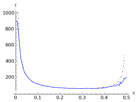
Figure 6: Classification time for $\mathcal{B}(101,10)$ depending on $\eta$, empirical and as approximation. The dashed line is the approximated classification time (71) and the straight line represents the measured values. For every value of $\eta$, the simulation was run 200 times over 900 time steps and the resulting times then averaged. Failed classifications were counted as if requiring 900 time steps.

Figure 6 compares the approximation (71) of the classification time with the empirical values for different $\eta$. The approximated classification time was good for $0.01<\eta<0.4$, and the actual classification time was always less than or equal to the predicted time.

A curve similar to that in Figure 6 was found empirically by Fatès [4, Figure 4] for arbitrary initial configurations. Fatès also found that the classification time has its minimum at $\eta\approx 0.3$. We can see the same minimum in Figure 6.

There is also theoretical justification: For a given $\ell$, the recognition time function in (71) takes its minimum at $\eta=\frac{2\ell-\sqrt{2\ell(\ell-1)}}{2(l+1)}$. If $\ell$ is large, this expression simplifies to $1-1/\sqrt{2}\approx 0.294$, close to the empirical values.

Initial Density

The connection between the initial density and the quality of the approximation was investigated by two experiments.

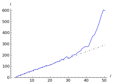
Figure 7: Classification time for $\mathcal{B}(101,\ell)$ depending on $\ell$, for $\eta=0.3$. The other parameters are the same as in Figure 6.

In the first experiment (Figure 7), the ring size $n$ was kept fixed and the length $\ell$ of the initial block varied. The approximated classification time was reasonably good for $\ell$ less than about 40, corresponding to an initial density of 0.4. For higher values of $\ell$ the actual classification time was larger than the time predicted by the model.

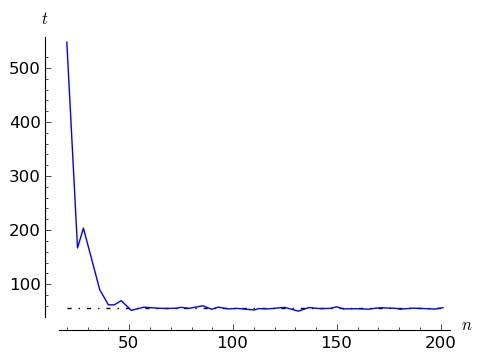
Figure 8: Classification time for $\mathcal{B}(n,10)$ depending on $n$, for $\eta=0.3$. The other parameters are the same as in Figure 6.

In the second experiment (Figure 8), the length of the initial block was kept fixed at a value of 10 and the ring size $n$ varied. Here the quality of the approximation was good for $n$ greater than approximately 40, corresponding to a density of 0.25. For $n<40$, the actual classification time was always larger than the predicted time, mostly by a large amount.

Ring Size

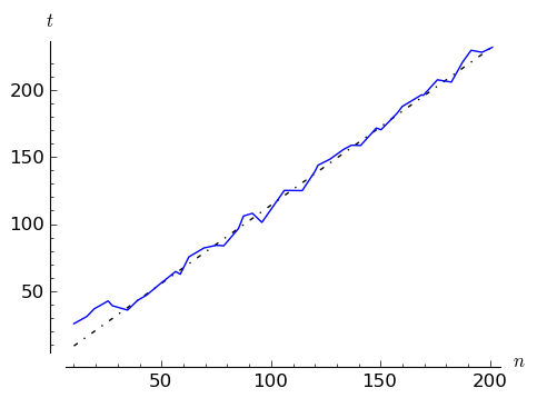
Figure 9: Classification time for $\mathcal{B}(n,\lfloor 0.2n\rfloor)$ depending on $n$, for $\eta=0.3$. The other parameters are the same as in Figure 6.

A final experiment shows the influence of the ring size $n$ on the quality of the approximation. The ring size does not even appear in the approximated model, and we can ask whether that omission was justified.

The results of the experiment are shown in Figure 9. Here the ring size varied and the initial density was always 0.2. There was no visible influence of $n$ on the quality of the approximation in the data.

6 Discussion of the Results

6.1 Experimental Data

The most surprising result is certainly the good quality of the approximation in Figure 6. It seems that the assumption that the non-crossing path pairs are the most important contributors to the behaviour of $\vec{B}^{\mathbb{Z}}$ is justified by the data, even for relatively large $\eta$.

On the other hand, the omission of the “early wraparound” from the analysis, i. e. the assumption that the right end of the 01-sequence never interacts with the left end of the 1-block during Phase I, was not in the same measure justified by the data. Only for initial densities less than 0.4 or even 0.25 (depending on whether one trusts Figure 7 or 8 more), the approximation is good. There must be a quite large space left at the right side of the initial $\mathcal{B}(n,\ell)$ to make sure that no significant wraparound occurs.

From Figure 9 we finally derive a different kind of result: It shows that already for relatively modest ring sizes, like $n\geq 50$, the actual value of $n$ is no longer important. In cellular automata with transition rule $\varphi_{\eta}$, the cells then play the role of atoms, or of cells in biology, and are so small that their number becomes unimportant.

6.2 Conclusion

We see that already this simplified model captures significant properties of the traffic-majority rule. The derivation of the results is however still quite complex, even for the simplified model. In future, this kind of derivation could certainly be streamlined.

A puzzling fact is that the model, developed for the the evolution of a single block, also describes the behaviour of arbitrary initial configurations reasonably well. Apparently the traffic-majority rule behaves as if every initial configuration were a sequence of blocks that evolved independently of each other. A theoretical justification of this idee would considerably simplify the analysis of this and other cellular automata.

Acknowledgements

This paper was originally created as a part of an university module under the guidance of Tim Swift. Many thanks to him, especially for the advice to restrict the analysis of the traffic-majority rule to the behaviour of blocks. I also want to thank Nazim Fatès for reading a late draft and giving helpful hints.

References

- [1] Raimundo Briceño, Pablo Moisset de Espanés, Axel Osses, and Ivan Rapaport. (2013). Solving the density classification problem with a large diffusion and small amplification cellular automaton. Physica D, 261:70–80.
- [2] Mathieu S. Capcarrère, Moshe Sipper, and Marco Tomassini. (1996). Two-state, cellular automaton that classifies density. Physical Review Letters, 77(24):4969–4971.
- [3] Nazim Fatès. (2011). Stochastic cellular automata solve the density classification problem with an arbitrary precision. In Thomas Schwentick and Christoph Dürr, editors, 28th International Symposium on Theoretical Aspects of Computer Science (STACS 2011), volume 9 of Leibniz International Proceedings in Informatics (LIPIcs), pages 284–295, Dagstuhl, Germany. Schloss Dagstuhl–Leibniz-Zentrum für Informatik.
- [4] Nazim Fatès. (2013). Stochastic cellular automata solutions to the density classification problem: When randomness helps computing. Theory of Computing Systems, 53:223–242.
- [5] Henryk Fukś. (1997). Solution of the density classification problem with two cellular automata rules. Physical Review E, 55(3):R2081–R2084.
- [6] Henryk Fukś. (2002). Nondeterministic density classification with diffusive probabilistic cellular automata. Physical Review E, 66(6):066106.
- [7] P. Gács, G. L. Kurdiumov, and L. A. Levin. (1987). One-dimensional homogenous media dissolving finite islands. Problemy Peredachy Informatsii, 14:92–98.
- [8] Ronald L. Graham, Donald E. Knuth, and Oren Patashnik. (1989). Concrete Mathematics. Addison-Wesley Publishing Company.
- [9] Geoffrey R. Grimmett and David R. Stirzaker. (1989). Probability and Random Processes. Clarendon Press.
- [10] Mark Land and Richard K. Belew. (1995). No perfect two-state CA for density classification exists. Physical Review Letters, 74(25):5148–5150.
- [11] Chris G. Langton. (1990). Computation at the edge of chaos: Phase transitions and emergent computations. Physica D, 42:12–37.
- [12] Melanie Mitchell. (1998). Cellular automata: A selected review. In Timo Gramß, Stefan Bornhold, Michael Groß, Melanie Mitchell, and Thomas Pellizari, editors, Non-Standard Computation, pages 95–140. Wiley-VCH.
- [13] Melanie Mitchell, James P. Crutchfield, and Peter T. Hraber. (1994). Evolving cellular automata to perform computations: Mechanisms and impediments. Physica D, 75:361–391.
- [14] Melanie Mitchell, Peter T. Hraber, and James P. Crutchfield. (1993). Revisiting the edge of chaos: Evolving cellular automata to perform computations. Complex Systems, 7:89–130.
- [15] N. H. Packard. (1988). Adaptation toward the edge of chaos. In J. A. S. Kelso, A. J. Mandell, and M. F. Schlesinger, editors, Dynamic Patterns in Complex Systems, pages 293–301. World Scientific, Singapore.
- [16] M. Sipper, M. S. Capcarrère, and E. Ronald. (1998). A simple cellular automaton that solves the density and ordering problems. International Journal of Modern Physics C, 9(7):899–902.
- [17] Stephen Wolfram. (1983). Statistical mechanics of cellular automata. Reviews of Modern Physics, 55:601–644.