The PBR theorem seen from the eyes of a Bohmian

Abstract

The aim of this paper is to present an analysis of the new theorem by Pusey, Barrett and Rudolph (PBR) concerning ontic and epistemic hidden variables in quantum mechanics PBR ; Leifer1 . This is a kind of review and defense of my previous critical analysis done in the context of Bohmian mechanics. This is also the occasion for me to review some of the fundamental aspects of Bohmian theory rarely discussed in the literature.

I A not too ‘Bohring’ Introduction to Bohm (I hope)

I am a Bohmian (i.e. a ‘de Broglian’) which means somebody believing in the pertinence of the pilot wave theory proposed by de Broglie in 1926-27 and rediscovered by Rosen in 1945 and Bohm in 1952 (see the book by Holland Holland ). What is pilot wave theory? A completely deterministic and neat approach at the fundamental level involving trajectories and dynamical laws for point-like quanta (at least in its original version). This quantum interpretation which contrasts with the one proposed by Bohr Heisenberg and others is done in such a way as to agree completely with quantum mechanics rules and in particular is tuned to reproduce every statistical prediction given by the usual formalism (this is why we speak about an interpretation of the quantum formalism). The theory works not only for a single particle, but also for systems of several entangled objects (even though entanglement was not clearly defined in 1927) such as particle beams or molecules. Furthermore, the theory is completely nonlocal in the sense defined by Bell with his famous theorem of 1965. Therefore, the theory although deterministic is able to describe subtle quantum effects such as correlations (i.e., the EPR paradox) and interferences (i.e., the wave particle duality) and provides a clear ontology for understanding the quantum world by solving all the measurement paradoxes. The reaction to this proposition was from the beginning very emotional and the theory of de Broglie and Bohm was often named ‘metaphysical’ or ‘ideological superstructure’ and even recently accused of being ‘surrealistic’ (see for example refs. Scully ; Vaidman ). The main reasons for the strong opposition is that pilot wave says that things which are not experimentally determinable are however determined in a very precise way by dynamical laws (the so called guidance equations of de Broglie). But, since the pilot wave agrees with quantum mechanics it should also certainly accept the Heisenberg uncertainty and the results concerning wave particle duality with the double-hole experiment. How could that be? Indeed, pilot wave agrees with all that but in a very peculiar way. To understand that, I remind you briefly what is the point of view of Bohr and Heisenberg on this topic. The argumentation focuses on the famous double-hole interference experiment done with single electron or photon and which shows that a particle could be influenced by the hole through which it is not going to pass in order to create an interference pattern. This is a kind of paradox if we try to think in term of a particle path going from only one hole and which ‘obviously’ should not care about the ‘remote’ presence of the second hole. For Bohr and Heisenberg this paradox should be removed. ‘Fortunately’, they wrote, the presence of the ‘particle’, i.e., the ‘trajectory’ can not be detected at both holes without disturbing the fringes. Therefore, at least at the experimental level, no contradiction like to be at A and not at A at the same time can occur. Bohr and Heisenberg emphasize that the result is actually worst that a naive picture of the uncertainty principle could apriori let us to believe. Indeed, this naive semi-classical picture would say that the measurement always disturbs but that ‘OK we could still may-be preserve, at least conceptually, trajectories even if they are hidden’. However, quantum mechanics predicts that even a very small interaction which localize the particle, say in only one arm of an interferometer but not in the other (the spatial precision is not so huge here since the interferometer can be very big), will disturb and destroy the subsequent fringes. Therefore, it seems that hypothetical trajectories have no meaning in the experimental world, and since they can not be investigated they are metaphysical. Quantum mechanics textbooks are full of examples like the previous one discussed either in term of momentum ‘kicks’ à la Heisenberg or Feynman or involving more sophisticated devices and entanglement machineries. All the practitioners of the orthodox school generally emphasize that there is no other choice: in the quantum world we have to abandon our habits our clean logics and accept that things can not be fully described by the classical categories such as position $\mathbf{X}(t)$ and velocity $\dot{\mathbf{X}}(t)$ characterizing locally the system and evolving deterministically with time. Following Bohr and his complementarity principle one must choose which variable we want to experimentally define and we can then unambiguously calculate the probability of occurrence for such events using the quantum rules. However, these experimental contexts sometimes exclude each other (i.e., they are complementary like for example experimental arrangements for measuring either $x$ and $p$ for a same particle) and we must definitely renounce to our classical illusions such as trajectories and paths existing independently of the observation. Of course, the time evolution $\mathbf{X}(t)$ disappears completely from the discussion and we are allowed only to speak about the probability $dP(\mathbf{X},t)$ to observe the system with the value $\mathbf{X}$ at the time $t$. If we don’t measure $\mathbf{X}$ then it has no actualized reality; it was only a potentiality at the given time $t$. The subsequent evolution of the then undisturbed wave-function $|\Psi(t^{\prime})\rangle$ will give other potentialities at a future time $t^{\prime}$ which again will or not be actualized in our experimental world depending on your will to measure it or not.
If experimentally you can not determine a trajectory with a too large precision, i.e., at least nor large enough to observe both the path and fringes with a same particle, what could be the interest of such a pilot wave dynamics? This is a clear drawback of the Bohmian approach and it explains why it was so attacked strongly by Heisenberg, Pauli and many others. Although pilot wave solves in a neat way the measurement problem by fixing an ontology it also brings us parameters which somehow stay ‘hidden’ and therefore apparently metaphysical. However, I think this reaction exaggerated. First, we could remark that Heisenberg and Bohr are not completely fair concerning trajectories when they say that these paths have no existence. Actually, they go too far since their claim can not be proven either and are even contradicted by the pilot wave mere existence (as it was emphasized by de Broglie and Bohm in 1951-52). In particular, it is important to remind that von Neumann demonstrated in the 1930’s a famous theorem forbidding the existence of such a kind of hidden variable model and until the 1980’s it was often quoted as a final impossibility proof for the existence of trajectories, even though pilot wave was already a counter example, and even after Grete Hermann and later John Bell showed that the axiomatic of the theorem is not general enough to get to the von Neumann expected theorem. I think that the Copenhagen interpretation should be amended seriously at least on that point by replacing the world non existent by something like experimentally hidden without breaking the fringe coherence. But is this really true? Are particle paths completely hidden at the experimental level? This is not actually totally the case. In recent years much more was written on weak values as defined by Aharonov, Albert and Vaidman Albert and in particular on the possibility to identify a certain weak value $\mathbf{A}_{w}$ with the velocity field $\mathbf{\dot{X}}(t)$ attributed precisely by the pilot wave to the particle located at $\mathbf{X}(t)$. Actually, this was experimentally demonstrated Kocsis showing that the Bohmian trajectories can have an experimental reality. There is however no contradiction with what was find and discussed before. The trick is indeed to realize that a weak measurement is not done on a single individual unlike the strong projective measurement. Weak measurement is weak and requires a large population of particles to get the trajectories. Therefore, in all these examples the Heisenberg principle stays valid: we can not detect fringes and path for a same particle. Therefore, the sentence experimentally hidden means in reality experimentally hidden at the single particle level. But, I would like to point out that even this apparently prudent analysis is not exempt of critics. Indeed, beside the weak measurement protocol Aharonov and Vaidman also defined what they called a protective measurement protocol Vaidman2 . This is a very interesting method focussing on the fact that in some conditions we can define a system $S$ evolving very slowly and gently (i.e. adiabatically) which can be coupled to a meter which evolves very strongly into a well distinguishable state. The result of the protocol will not give us a way to record precisely the spectrum of an observable $A$ of the system (i.e. unlike in a von Neumann protocol) but either, will give us the new possibility to measure its average value $\langle\psi_{S}|A|\psi_{S}\rangle$. This is very interesting in the context of pilot wave for several reasons. First, since $\langle A\rangle$ can be for example the probability density $\rho(\mathbf{X}_{0})=\langle\psi_{S}|\mathbf{X}_{0}\rangle\langle\mathbf{X}_{0}|\psi_{S}\rangle$ or the current $J(\mathbf{X}_{0})=\langle\psi_{S}[|\mathbf{X}_{0}\rangle\langle\mathbf{X}_{0}|\mathbf{P}-\mathbf{P}|\mathbf{X}_{0}\rangle\langle\mathbf{X}_{0}|]/(2mi)|\psi_{S}\rangle$ of the particle (with mass $m$) at point $\mathbf{X}_{0}$, one could at first argue (like in ref. Aharonov ) that the protocol proves once again the surrealistic nature of the Bohmian trajectories. Indeed, the protective measurement protocol can be used to ‘detect’ the particle at points where the Bohmian particle never approaches. This reasoning is based on the fact that for a real wave function $\langle\mathbf{X}|\psi_{S}\rangle$ the Bohmian particle is not moving at all (i.e., $\dot{\mathbf{X}}(t)=0$) so that even if the particle is fixed at position $\mathbf{X}_{1}\neq\mathbf{X}_{0}$ the protective measurement will allow to measure $\rho(\mathbf{X}_{0})$. How could that be? Although I will not here answer to that in details I can provide a simple qualitative explanation: particle is not everything in the pilot wave. For a Bohmian the wave is also a fundamental ingredient so that the force exerted on a particle depends not only on the ‘contact’ potential proposed in ref. Aharonov but also on a quantum potential which can acts in some non classical but completely deterministic way. This is enough to justify how the dynamics of the pointer is affected in some nonlocal way by the quantum interaction. I actually developed a complete Bohmian reasoning in Drezet as a reply to ref. Aharonov , see also the forthcoming chapter in the Book ‘Protective Measurement and Quantum Reality’ edited by Shan Gao Gao ). There is however an other reason why protective measurement is interesting in the context of Bohmian mechanics. Although I didn’t emphasized that point enough in the past this is actually much more important. Indeed, protective measurement is done at the single particle level which means that even a single pointer measurement allows us to determine $\rho(\mathbf{X}_{0})$ or $J(\mathbf{X}_{0})$. But since the operators associated with $\rho(\mathbf{X}_{0})$ or $J(\mathbf{X}_{0})$ commute actually nothing forbid us to measure $\rho(\mathbf{X}_{0})$ and $J(\mathbf{X}_{0})$ together (for example with two pointers). But now, for a Bohmian this is a bit of magic because we have a way to measure at the single particle level the ratio $J(\mathbf{X}_{0})/\rho(\mathbf{X}_{0})$ which is nothing else that the particle velocity. It is thus not anymore justified to say that the Bohmian velocity is not an observable. Of course in someway the Heisenberg uncertainty principle is not in question since the protective measurement is not a projective detection of the particle position at $\mathbf{X}_{0}$. We don’t have access to the actual trajectory followed by the particle because knowing the velocity is not enough: we should also have the actual position but this would require a projective method. However, we could imagine the following operations: first make a protective measurement to obtain the velocity at $\mathbf{X}_{0}$, then measure projectively for the same particle its position $\mathbf{X}$. Subsequently, retain only those cases where the projective measurement gives $\mathbf{X}=\mathbf{X}_{0}$. We have thus both the particle and velocity for the same particle at the same time! Note that the future evolution will be however random since the projective measurement is very intrusive. Still, this result is I think remarkable. I point out that it relies on the definition of the time scales involved in the process. Indeed, if by protective we mean adiabatic and very slow then the complete two-measurements procedure proposed here will have only meaning if the Bohmian velocity is very small so that it will still makes perfectly sense to speak about a velocity and position recorded at the same time for one particle.
There are other reasons for defending Bohmian mechanics. One of them is that it provides finally a kind of intelligibility which is absent from the Copenhagen interpretation. Indeed, since for Bohr we can not say anything about the system between measurements, it means, like it was shown by Wigner, that an observer can stays in a ubiquitous quantum state without clean ontological status before a second observer finalizes his experiment. How could that be and what does it mean? If we speak only about epistemic there is no real problem since knowledge is indeed relative. However, if we speak about ontology this is a non sense (this is also the main message of the Schrodinger cat paradox I think). But if we follow Heisenberg and his quantum/classical ‘cut’ this conclusion is unavoidable. Ultimately, the Universe as a whole becomes an issue. Does god existence (with a Ph.D) proven to be necessary for collapsing the wave function of the Universe? This seems extremely difficult to believe for me. This is an example of twilight zone which surrounds Bohr-Heisenberg interpretation and this the reason why for me Bohmian is superior to Copenhagen. Still, one could perhaps criticize Bohmian mechanics on a different level. I remind indeed that for a non relativistic particle of mass $m$ the pilot wave particle velocity is given by the de Broglie guidance formula

$$\frac{d}{dt}\mathbf{X}(t)=\frac{\hbar}{2mi}\Psi(\mathbf{X},t)^{\ast}\stackrel{{\scriptstyle\leftrightarrow}}{{\boldsymbol{\nabla}}}\Psi(\mathbf{X},t)/|\Psi(\mathbf{X},t)|^{2}=\frac{\mathbf{J}(\mathbf{X},t)}{|\Psi(\mathbf{X},t)|^{2}}$$ (1)

where $\mathbf{J}$ is the Madelung probability current arising from Schrödinger equation. However, from local conservation we have $\boldsymbol{\nabla}\cdot\mathbf{J}(\mathbf{X},t)+\partial_{t}|\Psi(\mathbf{X},t)|^{2}$. It is thus clear that we can add a rotational $\boldsymbol{\nabla}\times\mathbf{C}(\mathbf{X},t)$ to the current without changing the conservation. How could we be sure that our velocity formula is the good one? Pilot wave can not answer that univocally without calling to an other principle. For example one could try to invoke some Galilean or Lorentzian symmetries or principles Durr . We could also invoke weak measurement or protective measurement for giving an empirical support to some Bohmian concept not anymore so hidden. The answer to be given for this lack of univocity is not clear but for me it actually means that Bohmian mechanics is only a temporary expedient waiting for something of better, i.e., for a theory in which the pilot wave dynamics will appear as a consequence more than a postulate. An other element leads to the same conclusion: the wave acts on the particle but the reciprocal is not true. Therefore, it seems that the Bohmian quantum force is only an effective trick and that something of deeper is hidden here waiting for further investigations and discoveries (may be along the path proposed by de Broglie with its double solution program). I also mention a difficulty with the energy concept: For a general quantum state the actual Bohmian Energy defined by $E=-\partial_{t}S(\mathbf{X},t)$, where $S/\hbar$ is the wave function local phase, is not in general a constant even in the absence of any external potential. It is for me very difficult to accept such a feature for a final theory: the total energy should be a constant in the absence of external forces. Probably the energy definition is not so good here. This again, motivates for further investigations beyond the pilot wave. In the same vain, sometimes the Bohmians speak about ‘empty waves’ Hardy when for example a wave pack splits into several branches and when a particle chooses only one. The others branches are clearly empty of particles but are the waves still there in the branches? If the quantum potential has a reality independent of the particle the answer is ‘yes! certainly ’ but there is no proof of that and empty waves have not been directly detected yet. Once again, I think these are strong arguments for going beyond the pilot wave approach and that quantum mechanics will be superseded by something else (this was the conviction of de Broglie by the way).
This is a long introduction to justify my quantum realist/determinist position. But it serves only as a motivation for the next short section where I will describe the PBR theorem and its relation with Bohmian mechanics. PBR is an important result obtained at the end of 2011 by Pusey Barret and Rudolph concerning the relation of epistemic and ontic in hidden variable theories. In the long tradition started with Bell (or more honestly von Neumann) its aims is to give experimental bounds to the allowed models that quantum realists can propose. Bell, focussed on non-locality, a feature of Bohmian mechanics, and PBR were interested by the experimental definition of epistemic models. I will shortly review the PBR result PBR (without the demonstration) and explains why pilot wave escapes the conclusions. Still the theorem is true if we add an axiom. I actually found this rather simple result already in 2011 immediately after that the preprint of PBR circulated on the web but the work was published only later for editorial reasons. I also discussed this subject with M. Leifer on his blog page early in 2012 Leifer1 (but we disagreed on the conclusion as it is also shown in his recent manuscript Leifer : the current paper is also a kind of reply to him). For more details on the proof the interested readers could find some of my earlier manuscripts on Arxiv (see refs.Drezet2 ; Drezet3 ) and compare with a independent work by M.Schlosshauer and A. Fine Fine who clearly discovered the same result independently and simultaneously.

II the PBR result and its meaning for a Bohmian

What is PBR theorem? the demonstration that epistemic models are forbidden in quantum mechanics. Why epistemic models? Epistemic or knowledge interpretations have a long tradition in quantum mechanics. Einstein was a strong defender of such approaches and for him it meant that quantum mechanics was a kind of statistical mechanics like in the classical world but waiting for something of better with a clean deterministic foundation (again like classical mechanics). For Einstein, quantum mechanics was a bit like thermodynamics before the works of Clausius, Maxwell and Boltzmann on statistical physics. Actually, this is not really different from the de Broglie and Bohm point of view and we should not forget that Einstein proposed already in 1907 that particle of light should be envisioned as a kind of singularity riding atop a guiding electromagnetic field (this is the de double solution program of de Broglie). De Broglie succeeded where Einstein failed and the pilot wave of de Broglie-Bohm indeed justifies the existence of probability by a statistical mechanical argument like Boltzmann or Gibbs did with Newton laws. By Epistemic models PBR meant actually a sub-class of this kind of statistical model but they didn’t realize it in their paper. Before to come to this let go to the first step of the PBR theorem which is purely quantum in the sense of the formalism. In the simplest version PBR considered two non orthogonal pure quantum states $|\Psi_{1}\rangle=|0\rangle$ and $|\Psi_{2}\rangle=[|0\rangle+|1\rangle]/\sqrt{2}$ belonging to a 2-dimensional Hilbert space $\mathbb{E}$ with basis vectors $\{|0\rangle,|1\rangle\}$. We will limit ourself to this example for the discussion since the details are not so important here. Using a specific measurement protocol $M$ with basis $|\xi_{i}\rangle$ ($i\in[1,2,3,4]$) in $\mathbb{E}\otimes\mathbb{E}$ which precise form is here irrelevant (see ref.PBR ) PBR deduced that $\langle\xi_{1}|\Psi_{1}\otimes\Psi_{1}\rangle=\langle\xi_{2}|\Psi_{1}\otimes\Psi_{2}\rangle=\langle\xi_{3}|\Psi_{2}\otimes\Psi_{1}\rangle=\langle\xi_{4}|\Psi_{2}\otimes\Psi_{2}\rangle=0$. which means that some probabilities cancel with such protocols. Now in order to see the contradiction we go to the second step and try to introduce an hypothetical hidden variable model reproducing the statistical features of quantum mechanics. This is clearly the classical methodology proposed by Bell. Bell introduced ‘hidden variables’ $\lambda$ which in the Bohmian language could be the possible coordinates of the particles at the initial time. Here, I will be more precise that PBR because I want to emphasize later some limitations on the reasoning. First, consider a quantum state $|\Psi\rangle$ and an observable $A$ with eigenvalue $\alpha$. The probability of occurrence for $\alpha$ will be given by

$$|\langle\alpha|\Psi\rangle|^{2}=P(\alpha,\mathbf{a}|\Psi)=\int P(\alpha,\mathbf{a}|\lambda)\rho(\lambda|\Psi)d\lambda.$$ (2)

In this notation we introduced the hidden variable distribution $\rho(\lambda|\Psi)$ and the conditional probability $P(\alpha,\mathbf{a}|\lambda)$ (such as $\sum_{\alpha}P(\alpha,\mathbf{a}|\lambda)=1$ by definition of a conditional probability) defining the ‘likehood’ for the system to evolve from its initial state (characterized by its hidden variable $\lambda$, and its wave function) to a state where the eigenvalue $\alpha$ will be actualized (i.e. after a projective measurement characterized by some external parameters $\mathbf{a}$ such as the spin analyzer direction in a Stern Gerlach experiment). These definitions are very classical-like since the dynamic or ‘ontic’ state should be decoupled from its epistemic counterpart in agreement with the Boltzmann-Gibbs statistical approach. Of course, $\rho(\lambda|\Psi)$ is supposed to be independent of $\mathbf{a}$ since causality is expected to hold from past to future and if your reject retro-causal, some ‘magical’ conspiracy or super deterministic approaches à la Costa de Beauregard or John Cramer (e.g., the very interesting transactional interpretation). Now, in the PBR reasoning we should write

$$|\langle\xi_{i}|\Psi_{j}\otimes\Psi_{k}\rangle|^{2}=\int P_{M}(\xi_{i}|\lambda,\lambda^{\prime})\varrho_{j}(\lambda)\varrho_{k}(\lambda^{\prime})d\lambda d\lambda^{\prime}$$ (3)

where $i\in[1,2,3,4]$ and $j,k\in[1,2]$. Actually, in their paper PBR didn’t use such notations but these obviously simplify the reasoning like they did for Bell. In this PBR model there is an independence criterion at the preparation since we write $\varrho_{j,k}(\lambda,\lambda^{\prime})=\varrho_{j}(\lambda)\varrho_{k}(\lambda^{\prime})$. This is a very natural axiom and for example such an axiom would be justified in the Bohmian interpretation where the hidden parameters are the initial coordinates $\mathbf{X}_{1}(0)$ and $\mathbf{X}_{2}(0)$ of the particles in the incident wave-packets (Although we are here speaking about Q-bit this is not a problem: Bohm works also for spins but here the Q-bits could simply belong to a sub-manifold of the full hilbert space like it is for instance with two-energy-level systems. Therefore, spatial coordinates are still relevant). In these equations we again introduced the conditional ‘transition’ probabilities $P_{M}(\xi_{i}|\lambda,\lambda^{\prime})$ for the outcomes $\xi_{i}$ supposing the hidden state $\lambda,\lambda^{\prime}$ associated with the two independent Q-bits are given. The fundamental point here is that $P_{M}(\xi_{i}|\lambda,\lambda^{\prime})$ is independent of $\Psi_{1},\Psi_{2}$. Obviously, we should have $\sum_{i=1}^{i=4}P_{M}(\xi_{i}|\lambda,\lambda^{\prime})=1$. It is then easy using all these definitions and conditions to demonstrate that we must necessarily have

$$\varrho_{2}(\lambda)\cdot\varrho_{1}(\lambda)=0 \forall\lambda,$$ (4)

i.e., that $\varrho_{1}$ and $\varrho_{2}$ have nonintersecting supports in the $\lambda$-space. This constitutes the PBR theorem for the particular case of independent prepared states $\Psi_{1},\Psi_{2}$ defined before (but PBR generalized their results for more arbitrary states using similar and astute procedures described in ref. PBR ). What are the implications of such a result? If we identify the conditions imposed by PBR on the hidden variable models with what should be naturally expected from any ontological model having a statistical ingredient, then we could conclude that such models are nor really statistical. Indeed, from Eq. 4 we deduce that the density of probabilities $\varrho_{\Psi_{1}}(\lambda)$ $\varrho_{\Psi_{2}}(\lambda)$ for any two quantum states $\Psi_{1}$ and $\Psi_{2}$ are necessarily not overlapping in the $\lambda-$(phase) space. Therefore, it will be like if we have necessarily a delta distributions $\delta^{3}(q-X(t))\delta^{3}(p-P(t))$ in classical mechanics. This kind of model could hardly be called statistical at all? If this theorem is true (and mathematically it is) then it would apparently make hidden variables completely redundant since it would be always possible to define a relation of equivalence between the $\lambda$ space and the Hilbert space: (loosely speaking, we could in principle make the correspondence $\lambda\Leftrightarrow\psi$). In other words, it would be as if $\lambda$ is nothing but a new name for $\Psi$ itself!
However the PBR reasoning doesn’t fit with the Bohmian mechanics framework and therefore it is not difficult to see that the reasoning obtained by PBR can not hold for such a theory. First, observe that for pilot wave we have both $\mathbf{X}(t)$ and $\Psi(\mathbf{X},t)$ as ontological variables and since Born’s rule occurs then by definition $\rho_{\Psi}(\mathbf{X},t)=|\Psi(\mathbf{X},t)|^{2}$ defines in the pilot wave model the probability of presence for the particle. If we consider the initial state at the initial time $t_{0}$ we have $\rho_{\Psi}(\lambda):=|\Psi(\mathbf{X},t_{0})|^{2}$. This is an epistemic distribution of hidden variables guided by the wavefunction $\Psi(\mathbf{X},t)$. Clearly, for two given states $\Psi_{1}$ and $\Psi_{2}$ (orthogonal or not) we have in general $\rho_{\Psi_{1}}(\lambda)\cdot\rho_{\Psi_{2}}(\lambda)\neq 0$ in contradiction with Eq. 4 and PBR statement. To see why it is like that we first point out that Bohm model is deterministic. Therefore, for a given $\lambda_{0}:=\mathbf{X}(t_{0})$ we know that the evolution of the system in a projective measurement will also be deterministic. After the measurement is done the particle is actually in one of the allowed eigenvalues $\alpha_{0}$ (supposed discrete here for simplicity) and we can write $\alpha_{0}=A(\lambda_{0},\mathbf{a},\Psi_{0})$. We should consequently write Eq. 2 with

$$P\left(\alpha|\mathbf{a},\lambda,\Psi_{0}\right)=\delta_{\alpha,A(\lambda,\mathbf{a},\Psi_{0})}=0\textrm{ or }1$$ (5)

where $\delta$ is the Kronecker symbol, since for one given $\lambda$ only one trajectory is allowed (this model of course satisfies trivially the condition $\sum_{\alpha}P(\alpha|\mathbf{a},\lambda,\Psi_{0})=1$). Equivalently, the actual value $A(\lambda,\mathbf{a},\Psi_{0})=\sum_{\alpha}\alpha P\left(\alpha|\mathbf{a},\lambda,\Psi_{0}\right)$ can only takes one of the allowed eigenvalues $\alpha$ associated with the hermitian operator $A$. Such kind of notations were used by Holland in his book Holland (see also vigoureux ). What is fundamental here is that Eq. 5 depends on $\Psi_{0}$(the initial wave function) in a explicit way. Still, beside this contextually the Bohm model is a clean statistical model and there is no reason which can forbid us to call it an epistemic model. This discussion shows however that pilot wave is not a banal classical model it contains a wave function $\Psi_{0}$ which have a particular status: it guides the particle and at the same time it characterizes completely the statistical ensemble for a given protocol. While, $\lambda$ can fluctuate in the ensemble (corresponding to the different possible values for $\mathbf{X}(t_{0})$) $\Psi_{0}$ is instead a kind of dynamical constraint belonging to an ensemble like was the action or the energy in the old Hamilton-Jacobi theory: $\Psi$ guides the particles and characterize the statistical ensemble footnote . Moreover, Eq. 2 is now modified and we should write

$$|\langle\alpha|\Psi\rangle|^{2}=\int\delta_{\alpha,A(\lambda,\mathbf{a},\Psi_{0})}\rho(\lambda|\Psi)d\lambda.$$ (6)

to take into account Eq. 5. Clearly, this means that PBR Eq. 3 should be modified as well to include this new contextual feature:

$$|\langle\xi_{i}|\Psi_{j}\otimes\Psi_{k}\rangle|^{2}=\int P_{M}(\xi_{i}|\lambda,\lambda^{\prime},\Psi_{j},\Psi_{k})\varrho_{j}(\lambda)\varrho_{k}(\lambda^{\prime})d\lambda d\lambda^{\prime}.$$ (7)

However, now we have lost the secret ingredient allowing us to obtain Eq. 4 which implies that the PBR derivation doesn’t hold anymore! (details are discussed elsewhere Drezet2 ; Drezet3 . Part of the language used here was also introduced long ago by Fine  Fine2 and discussed by me in a different context  vigoureux ; Drezet4 ). What does it mean? The ontic-epistemic framework used by PBR suggested that there is a clean separation between ontic and epistemic approaches. This is motivated by the PBR sentence ‘The statistical view of the quantum state is that it merely encodes an experimenter’s information about the property of a system. We will describe a particular measurement and show that the quantum predictions for this measurement are incompatible with this view’ PBR . By ‘merely’ PBR meant certainly something like classical statistical mechanics but what about Bohmian theory? Are they really ontic for them? Does PBR simply ignore it? I found that suspicious since Harrrigan-Spekkens start their paper speckens (cited in PBR ) by the following definition: ‘We call a hidden variable model $\psi-$ontic if every complete physical or ontic state in the theory is consistent with only one pure quantum state; we call it $\psi-$ epistemic if there exist ontic states that are consistent with more than one pure quantum state’. Now, as explained, Bohmians proposed since 1927 statistical interpretations where the wavefunction plays a dual role. $\Psi$ guides the particles but also justify the quantum statistical observations with some clear epistemic elements. Clearly , for a Bohmian the wavefunction is definitely not only a simple label to our epistemic knowledge but it is any way also such a label! In agreement with the previous quotation I would thus say that pilot wave is in part also epistemic but this is not actually the case in the ontological framework of these authors. They actually classified Bohmian mechanics as ‘$\psi$-supplemented’ (a sub class of ‘$\psi$-ontic’) meaning that additionally to $\Psi(\mathbf{x},t)$ we must add some hidden supplementary variables $\mathbf{X}(t)$. Somehow, I could agree also with this second definition which seems however to contradict my previous choice. So what! Is Bohmian mechanics epistemic or ontic? This is very confusing (i.e., not only for me; see for example Feintzeig Feintzeig who is also clearly disturbed by that). Since, the paper speckens played an important role in the work of PBR I think that there is a kind of language ambiguity in the reasoning. May be, PBR could reply to the critics by saying like Leifer (in his analysis of the work by me and M. Schlosshauer and A. Fine: ref. Leifer pages 60-63): ‘if your conditional probabilities for measurement outcomes depend on the wavefunction then the wave function is ontic and there is nothing left to prove.’ I indeed received few emails along that direction. However, for me the central point is not that the wave function is ontic (I have no doubt about that: see the first sentence of this article), but that epistemic is not orthogonal to ontic and that therefore the wave function is also an epistemic carrier. Interestingly, Leifer agrees in the same paper that ‘the scope of the PBR theorem is restricted to the case where this conditional independence holds’. However he then adds: ‘ but this is part of the definition of the term “ontic state”, rather than something than can be eliminated in order to arrive at a more general notion of what it means for a model to be $\psi-$epistemic that still conveys the same meaning’. In other words he recognizes that the PBR derivation doesn’t hold if you reject the $\Psi-$independence in the conditional probabilities but that I modified the definition of epistemic used by PBR. Clearly, we don’t have the same definition of what is to be ontic and epistemic. For me Bohmian mechanics is both ontic and epistemic while for Leifer and some others it is purely ontic. This looks like a old problem of semantic. Semantic plays indeed a role in this debate. PBR, Leifer and others call ontic respectively what M. Schlosshauer and A. Fine Fine called ’segregated models’ and ‘mixed models’. I clearly prefer the vocabulary of M. Schlosshauer and A. Fine although personally I would simply use something like non overlapping and overlapping distributions instead of segregated and mixed (this would agree with the figure 1 of the PBR paper PBR , see also Leifer1 ). Also, I completely agree with them Fine when they wrote: ‘we find this terminology less charged than the terms “$\psi$-epistemic” and “$\psi$-ontic” that PBR adopt from speckens [my reference]’. In particular, epistemic is very much charged in the context of probability theory where the objective or subjective nature of the concept is often debated. Furthermore, in classical mechanics even a simple trajectory is a solution of Liouville equation and corresponds to an ‘epistemic’ density of probability $\rho(q,p,t)=\delta^{3N}(q-X(t))\delta^{3N}(p-P(t))$ associated with a perfect knowledge. For the word ontic the situation is even worst. Ontic, is a philosophical word and its definition is a bit like God: everyone knows what it means but nobody agrees…I suggest that the use of such a charged vocabulary is responsible for the confusion surrounding this PBR theorem, therefore semantic is indeed here a problem. In the same vain, I would like to precise that I first learned about the PBR theorem version mainly through the Arxiv 2011 preprint of the PBR manuscript (compare with the final manuscript PBR ) and from the early pedagogical presentation by Leifer Leifer , and Barrett (done at Oxford the 12^th of March 2012 Barrett ). In all these works, the authors clearly consider the opposition ontic-epistemic in the sense segregated-mixed which is unambiguous. However, nowhere the postulate that $P(\alpha|\mathbf{a},\lambda)$ should be independent of $\Psi_{0}$ is even mentioned. This is the reason why I can fairly conclude that they didn’t included this axiom in their reasoning. For example Barrett mentions at slide 15 of his presentation that $P(\alpha|\mathbf{a},\lambda)$ is a natural axiom of Bell whereas Bell never postulated such a constraint. Furthermore, at slides 16-17 the opposition ontic$\Leftrightarrow$epistemic is done in such a way as to oppose the non-overlapping$\Leftrightarrow$overlapping distribution like if every thing was there. But, since the missing postulate $P(\alpha|\mathbf{a},\lambda,\Psi_{0})\Leftrightarrow P(\alpha|\mathbf{a},\lambda)$ is not mentioned it seems to play no role at all in the reasoning (this is not surprising since it doesn’t appear either in the Harrigan-Spekkens paper speckens ). However, once again, the opposition $P(\alpha|\mathbf{a},\lambda,\Psi_{0})\Leftrightarrow P(\alpha|\mathbf{a},\lambda)$ has a clear ontological and epistemic status (as important that the one associated with the overlapping or non overlapping density of states) and it must not be neglected otherwise the theorem is simply incomplete. We can also better appreciate this point by comparing  PBR ; Leifer ; Barrett with refs. Fine ; Fine2 ; Drezet4 where a clear discussion of what it means to include $\Psi_{0}$ in the probability $P(\alpha|\mathbf{a},\lambda,\Psi_{0})$ is done.
My critical analysis of the PBR theorem was however not intended to be semantical. It was not done for rejecting the complete PBR reasoning but only to show that the presentation of the theorem should be amended in order to make it general. The postulate that $P(\alpha|\mathbf{a},\lambda,\Psi_{0})$ should be independent of $\Psi_{0}$ is a critical part of the PBR derivation and should be explicitly included in order to see the limitations of the theorem and re-enforces his strength. Let me propose a version of the PBR theorem:
PBR theorem (amended version):
If $P\left(\alpha|\mathbf{a},\lambda,\Psi_{0}\right)$ is independent of $\Psi_{0}$ then Eq. 4 holds necessarily. In the opposite case this is not necessarily true.
The inclusion of this additional postulate concerning conditional probabilities has important consequences since it will shed some light on the properties of Bohmian mechanics (a bit like Bell’s theorem did).
Consider, for example the simple beam-splitter experiment shown on Figure 1. If we send a single photon state $|\Psi_{1}\rangle$ through the input gate 1. The wave packet splits and we will finish with a probability $P(3|1)=1/2$ to detect the photon in the exit 3

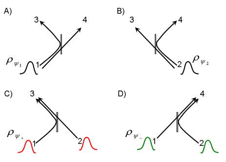
Figure 1: An example showing that the ‘old’ axiomatic of PBR can not be applied to a Bohmian like model. Cases A and B correspond to wave packets impinging from one of the 2 beam-splitter entrances. Exits 3 and 4 are both allowed. In case C and D where a superposition of wave packets interfere coherently the exits 4 and respectively 3 are forbidden. In Bohmian mechanics the hidden variable distributions from examples A and B overlap nevertheless with those of example C and D in contradiction with the PBR result (the problem is solved with the new axiomatic).

and identically $P(4|1)=1/2$ of recording the photon in exit gate 4. Alternatively, we can consider a single photon wave packet coming from gate 2 and at the end of the photon journey we will still get $P(3|1)=P(4|1)=1/2$. From the point of view of the hidden variable space we can write

$$P(4|1\textrm{ or }2)=\int P(3|\lambda)\rho(\lambda|\Psi_{1}\textrm{ or }\Psi_{2})=1/2$$ (8)

with ‘or’ meaning exclusiveness. Nothing can be said about the probabilities involved in the integral. Now, if we consider superposed states such as $|\pm\rangle=[|\Psi_{1}\rangle\pm i|\Psi_{2}\rangle]/\sqrt{2}$ the photon will finish either in gate 3 or 4 with probabilities $P(3|+)=P(4|-)=1$ and $P(4|+)=P(3|-)=0$. We here find us in the orthogonal case of PBR theorem (i.e. $\langle+|-\rangle=0$)Drezet3 . The deduction is thus straightforward and we get $\rho(\lambda|+)\rho(\lambda|-)=0$ for all possible $\lambda$ which means that the two densities of probability for superposed states can not have any common intersecting support in the $\lambda$-space. This is what we should conclude if we consider a model accepting the PBR axiom $P(\alpha|\mathbf{a},\lambda)$.
However, this is not what happens in the pilot wave approach. In this model where the spatial coordinates play a fundamental role we don’t have $\rho(\lambda|+/-)\rho(\lambda|\Psi_{2})=0$ neither we have $\rho(\lambda|+/-)\rho(\lambda|\Psi_{1})=0$ for every $\lambda$! Indeed, half of the relevant points of the wave packets $+$ or $-$ are common to $\Psi_{1}$ or $\Psi_{2}$. Actually, this is even worst since we also have $\rho(\lambda|+)\rho(\lambda|-)=\rho(\lambda|\pm)^{2}\neq 0$ for every $\lambda$ in the full $\lambda$-support (sum of the two disjoint supports associated with $\Psi_{1}$ and $\Psi_{2}$). This is in complete contradiction with PBR theorem ‘old’ axiomatic (i.e., not the version presented by me page 13). This is not surprising if we remember that with pilot wave we have $P(\alpha|\mathbf{a},\lambda,\Psi_{0})$ and not $P(\alpha|\mathbf{a},\lambda)$. For me what the PBR theorem shows is that somehow those classical-like models obeying to the PBR constraint $P(\alpha|\mathbf{a},\lambda)$ can not reproduce wave particle duality: these models are therefore trivially useless. This is actually not completely true because we are here sticking too much to the classical world with particle coordinates etc… If you reject that classical framework you can still find some good models reproducing the experiments and satisfying the PBR axiom $P(\alpha|\mathbf{a},\lambda)$ but they don’t look at all like classical physics (see my proposals Drezet2 ). However, if you want to conserve some classical features like paths and positions then you can use Bohmian mechanics but you will now have $P(\alpha|\mathbf{a},\lambda,\Psi_{0})$ instead of $P(\alpha|\mathbf{a},\lambda)$! Furthermore, the PBR theorem is for me very useful since if we accept to include explicitly the missing axiom discussed before then we deduce with PBR that the kind of ‘XIX^th century like’ epistemic model (i.e., imposing $P(\alpha|\mathbf{a},\lambda)$ but contradicting Eq. 4) are necessarily condemned.
What to conclude? I reviewed some of the fundamental aspects of the pilot wave approach and I discussed the PBR theorem within this context. Bohmian mechanics is for me the best available ontology, but it will certainly one day be superseded by a better theory justifying some of its magical assumptions. In this context PBR’s theorem, like Bell’s one, is very useful for discussing the pertinence of future and present hidden variable models. However, this theorem should be formalized in order to discuss the best existing models (like the one of de Broglie and Bohm) and therefore equipped with a satisfying axiomatic. When this is done correctly the difficult discussion concerning ontic and epistemic becomes easier and the theorem strength is nicely enforced.
Post-scriptum:
I would like to briefly discuss a consequence of the PBR theorem that M. Leifer Leiferblog called ‘the supercharged EPR argument’. This argument is also discussed in a recent paper by G. Hetzroni and D. Rohrlich Rohrlich (focussing on the relation between PBR and protective measurement; see also S. Gao Gao on this topic). The argument runs as follows. Take an EPR-like state i.e. a singlet state. This defines a pair of entangled Q-bits. Now, if you project one of the two remote Q-bits ‘Alice’ along a basis (i.e., using a Bell procedure) the second Q-bit ‘Bob’is projected in a specific state depending on the outcomes obtained for Alice. However, if you admit the PBR theorem but only consider, like Leifer did, the cases ‘$P(\alpha|\mathbf{a},\lambda)$’ (i.e. without the presence of $\Psi_{0}$) then you could conclude the following: The possible states of Bob are depending on the basis choices for Alice. These Bob states are different and in agreement with PBR these can not overlap in the $\lambda-$space (see Eq. 4). However, the basis choice for Alice can be done arbitrarily fast and therefore the Bob state will be collapsed with arbitrary huge velocity into its associated state. This would imply non-locality and this without involving Bell theorem! This is very nice, but now we see the interest of our new version of the PBR theorem: if we admit that the conditional probabilities can depend on the quantum state $\Psi_{0}$ the deduction doesn’t hold anymore because Eq. 4 is not true. Still, the conclusion is perhaps correct because if ‘$P(\alpha|\mathbf{a},\lambda)$’ becomes ‘$P(\alpha|\mathbf{a},\lambda,\Psi_{0})$’ we have apriori a clear non local feature from the start (Bohmian mechanics is nonlocal after all). In other words: projecting Bob in different states $\Psi_{i}$ means different dynamics ‘$P(\alpha|\mathbf{a},\lambda,\Psi_{i})$’ which are enforced non locally by the projection of Alice outcomes. It can be useful to be a bit more precise here. By ‘$P(\alpha|\mathbf{a},\lambda,\Psi_{i})$’ or ‘$P(\alpha|\mathbf{a},\lambda)$’ I mean the equivalent for the EPR case of the notation used in this paper. But, of course since we have two Q-bits and two sets of measurements characterized by -for example- Stern and Gerlach directions $\mathbf{a}$ (for Alice) and $\mathbf{b}$ (for Bob) we must precise a bit our notations. First, $P(\beta,\alpha|\mathbf{b},\mathbf{a})$ means the probability for finding the system with outcome $\alpha=\pm 1$ for Alice if her measurement device is aligned along $\mathbf{a}$ and $\beta=\pm 1$ for Bob if his measurement device is aligned along $\mathbf{b}$. I will omit the $\Psi_{0}$ notation for the singlet here since this is the same state during all the reasoning. Then, using the $\lambda$ notations we will get with Bell

$$P(\beta,\alpha|\mathbf{b},\mathbf{a})=\int P(\beta,\alpha|\mathbf{b},\mathbf{a},\lambda)\rho(\lambda)d\lambda.$$ (9)

We assume that $\rho(\lambda)$ is not depending on $\mathbf{a}$, $\mathbf{b}$ because we don’t like retro-causality (those who don’t agree could argue at that point) and we will therefore accept this simple causal condition. Now, the EPR-Leifer-PBR measurement is made in two steps: first, Alice is projected and we get $\alpha$, then Bob and we get $\beta$. For this reason we can instead of Eq. 9 write

$$P(\beta,\alpha|\mathbf{b},\mathbf{a})=\int P(\beta|\alpha,\mathbf{b},\mathbf{a},\lambda)dP(\alpha,\mathbf{b},\mathbf{a},\lambda)$$

$$=\int P(\beta|\alpha,\mathbf{b},\mathbf{a},\lambda)P(\alpha|\mathbf{b},\mathbf{a},\lambda)\rho(\lambda)d\lambda.$$ (10)

Now, we have many probabilities. The first one from the right is $\rho(\lambda)$ the density of probability in the initial hidden variable space. The second is $P(\alpha|\mathbf{b},\mathbf{a},\lambda)$ the conditional probability for going from the initial state to a state where Alice’s outcome is projected to $\alpha$. This rigorously depends on $\mathbf{a}$ and $\mathbf{b}$ but like for $\rho(\mathbf{b},\mathbf{a},\lambda)=\rho(\lambda)$ this will be simplified (using some causality prerequisites in this reference frame) to $P(\alpha|\mathbf{b},\mathbf{a},\lambda)=P(\alpha|\mathbf{a},\lambda)$ since the result of Alice can not depend on the not yet realized outcome of Bob and device $\mathbf{b}$ if space like separation is considered. Again, this is not a very general hypothesis (no retro-causality) but I only accept it in order to stick to the Bohmian framework. The last term is $P(\beta|\alpha,\mathbf{b},\mathbf{a},\lambda)$ the conditional probability to get $\beta$ for Bob knowing that we had $\alpha$ for Alice and that we started from $\lambda$. This is the PBR probability discussed before. It depends on the quantum state $\Psi_{i}:=|\alpha\rangle$ associated with the possible outcomes for Alice and depends also from the axes directions $\mathbf{a}$ and $\mathbf{b}$. But wait, how do I know that $P(\beta|\alpha,\mathbf{b},\mathbf{a},\lambda)$ should depend on $\mathbf{a}$ and $\alpha$ ? No, problem guys: simply take Bell’s theorem with its non locality proof. From Eqs. 9, 10 and Bell we have $P(\beta,\alpha|\mathbf{b},\mathbf{a},\lambda)=P(\beta|\alpha,\mathbf{b},\mathbf{a},\lambda)P(\alpha|\mathbf{a},\lambda)\neq P(\beta|\mathbf{b},\lambda)P(\alpha|\mathbf{a},\lambda)$ meaning that $P(\beta|\alpha,\mathbf{b},\mathbf{a},\lambda)$ should depends on a and $\alpha$. A detailed calculation in the context of Bohm theory would lead the same result. In other words accepting the different causality axioms used here Bell theorem is necessary anyway to get non locality. Few additional remarks are here important. First, Leifer considered the case where the conditional probabilities are not depending on the quantum state. From our own result this would imply that $P(\beta|\alpha,\mathbf{b},\mathbf{a},\lambda)$ is independent from a and $\alpha$ in apparent contradiction with Bell! However, this is not the case since it is not actually necessary to remove the dependence on a: only $|\alpha\rangle$ should be removed (in agreement with Leifer choice) so that Bell is safe and indeed non-locality holds. Therefore, from this reasoning it is difficult for me to see PBR as kind of proto-theorem able to create a ‘supercharged EPR argument’ since Bell is with us all along. A second remark concerns ‘wave function collapse’ in the regime involving Bohmian mechanics. Einstein, de Broglie, and Bohm didn’t like the wave function collapse: it looked as magic. Unless we introduce a nonlinear process, like GRW did, this is not physical. In the theory of de Broglie and Bohm there is no wave collapse. The different branches of the measuring process are all playing a role even those with an ‘empty wave’. Still, in the effective this is the same because the entanglement process between Alice and Bob breaks the coherence between the different possible states of Bob if one do a projective measurement on Alice. Every thing will be like if we have a statistical mixture which is somehow equivalent to a collapse since the quantum nature of the motion is now erased (in the sense of a ‘which-path’ experiment). Finally, I would like to point out that non-locality is in the current Bohmian theory a very curious thing. It clearly involves a kind of privileged reference frame or ‘Aether’ with a specific space-time foliation (see for example foliation ). This is not really covariant and we have the feeling to return to the Lorentz-Poincaré’s time when the relativity principle was clearly defined but when people tried to save a privileged frame anyway. For me this again motivates researches for a better theory.
I would like to thank M. Leifer, and the PBR authors for very interesting discussions in 2012. I would like to thank the CNRS for giving me the possibility to make at the same time experimental /theoretical physics in such ‘fashionable topics’ like quantum-plasmonics Nanoletters and letting me the opportunity to do fundamental physics.

References

- (1) M. F. Pusey, J. Barrett and T. Rudolph,‘On the reality of the quantum state’, Nature Phys. 8, 476 (2012). see also M. F. Pusey, J. Barrett and T. Rudolph, ‘The quantum state cannot be interpreted statistically’, arXiv:1111.3328.
-
(2)
M. Leifer, The quantum time 6, 1 (2011).
See the blog page [http://mattleifer.info/2011/11/20/can-the-quantum-state-be-interpreted-statistically/]. - (3) P. R. Holland, The Quantum Theory of Motion, Cambridge University Press, Cambridge, 1993. See also of course: D. Bohm, Part I, Phys. Rev. 85,166 (1952); Part II, 85 180 (1952). The fundamental work by de Broglie is discussed in L. de Broglie, J. Phys. Radium 8, 225 (1927) and in the report of the 5th Solvay’s conference (in french) reproduced recently in: G. Bacciagaluppi and A. Valentini (ed.s): Quantum Theory at the Crossroads - Reconsidering the 1927 Solvay Conference, Cambridge University Press (2007). The best book on the subject is still probably: D. Bohm and B. J. Hiley, The Undivided Universe - An Ontological Interpretation of Quantum Theory, Routledge, London (1993).
- (4) B. G. Englert, M. O. Scully, G. Süssmann, H. Walther, Z. Naturforsch. 47a (1992) 1175.
- (5) Y. Aharonov and L. Vaidman, About position measurements which do not show the Bohmian particle position, in: J. T. Cushing, A. Fine, S. Goldstein, Bohmian Mechanics and Quantum Theory: An Appraisal, Kluwer, Dordrecht, 1996, pp. 141-154.
- (6) Y. Aharonov, D. Z. Albert, and L. Vaidman , Physical Review Letters 60, 1351 (1988).
- (7) S. Kocsis, B. Braverman, S. Ravets, M. J. Stevens, R. P. Mirin, L. Krister Shalm, A. M. Steinberg, Science 332, 1170-1173 (2011).
- (8) Y. Aharonov, and L. Vaidman, Phys Lett. A 178, 38-42 (1993)
- (9) Y. Aharonov, B. G. Englert, and M. O. Scully, Phys. Lett. A 263, 138 (1999).
- (10) A. Drezet, Phys. Lett. A 350, 416-418 (2005).
- (11) A. Drezet in Protective Measurement and Quantum Reality Towards a New Understanding of Quantum Mechanics edited by Shan Gao, to appear in 2014, Cambrigde University press.
- (12) D. Dürr S. Teufel, Bohmian Mechanics, Springer(2009).
- (13) L. Hardy, Phys. Lett. A 167, 11-16 (1992).
- (14) M. Leifer, (2014) [http://arxiv.org/abs/1409.1570].
- (15) A. Drezet, Progress in Physics 4, 14 (2012). See also [http://arxiv.org/abs/1209.2565].
- (16) See my original manuscript deposited on Arxiv [http://arxiv.org/abs/1203.2475] the of March 2012, and also [http://arxiv.org/abs/1209.2862].
- (17) M. Schlosshauer and A. Fine, Phys.Rev. Lett. 108, 260404 (2012) and also the Arxiv manuscript [http://arxiv.org/abs/1203.4779v1] deposited the 21th of March.
- (18) A. Drezet, Opt. Commun. 250, 370 (2005).
- (19) T. Takabayasi, Prog. Theor. Phys. 8, 143 (1952).
- (20) M. de Gosson, The Principles of Newtonian and Quantum Mechanics: the Need for Planck’s Constant h; with a foreword by B. Hiley. Imperial College Press (2001).
-
(21)
Interestingly PBR in PBR mention classical dynamics and
define a physical property as something like the old Hamiltonian
which can take different values in different zones of the
phase space . However, if two values of the function
and can be associated to the same point this
is not for them a fundamental property but an epistemic quantity.
But, as it was pointed out long ago by
T. Takabayasi Takabayasi (in a beautiful paper) in classical
mechanics the Hamilton -Jacobi action defines such a
function (this is the beautiful subject of symplectic geometry). Two
different solutions and corresponding to two
different sub-ensembles of trajectories but characterized by the
same dynamics can be defined. By same dynamics I mean the
same Hamiltonian and therefore the same
possible trajectories defined by Hamilton’s equations:
The condition defines therefore different sub-ensembles for and which can be indeed called epistemic in agreement with PBR. Now, what is remarkable in Bohmian mechanics is that the Hamiltonian also depends on a quantum potential defined by the wavefunction in its polar form as(11)
This quantum potential modifies the dynamics since the Hamiltonian is now . Interestingly different wave functions mean in general different dynamics given by Hamilton’s law. Since and are coming together we see that we will have at the same time an ontic modification of the dynamics and an epistemic element defining a sub-ensemble of such a changing dynamics through the condition . This is a kind of technical reply for those, who like me, are very much in need for a clear and neat dynamical picture. Additionally, I would like to remind that Takabayasi Takabayasi (see also for example Holland Holland , and de Gosson deGosson ) showed that the Liouville density of probability in the phase space is in quantum mechanics given by . This is indeed an epistemic information but it clearly contains which like has a dual role in the theory (don’t forget that the density of probability in the space is given by and that it obeys to the ‘epistemic’ conservation law associated with Eq. 1 and defining the guidance law through the same equation).(12) - (22) A. Fine, Phys. Rev. Lett 48, 291 (1982).
- (23) This is old paper written in 2004 but never published: [http://arxiv.org/abs/0909.4200].
- (24) B. Feintzeig, Studies in history and philosophy of modern physics, to appear (2014).
- (25) N. Harrigan and R. W. Spekkens, Found. Phys. 40, 125 (2010).
- (26) J. Barrett, ‘What is the quantum state?’, QISW, Oxford, March 2012. The slides of the conference are available at [http://www.cs.ox.ac.uk/qisw2012/slides/barrett.pd]
- (27) M. Leifer, The quantum times [http://mattleifer.info/2012/02/26/quantum-times-article-on-the-pbr-theorem/].
- (28) G. Hetzroni, D. Rohrlich, [http://arxiv.org/abs/1403.1590].
- (29) S. Gao, ‘Notes on the reality of the quantum state’, [http://philpapers.org/rec/GAONOT] (2014).
- (30) D. Dürr, S. Goldstein, K. Münch-Berndl, N. Zanghì, Phys. Rev. A 60, 2729 (1999).
- (31) Few papers about my second life: A. Cuche et al., Nanoletters 10, 4566 (2010); O. Mollet et al. Phys. Rev. B 86, 045401 (2012); A. Drezet, C. Genet, Phys. Rev. Lett. 110, 213901 (2013).